Article

Subpixel Analysis of Primary and Secondary Infrared Emitters with Nighttime VIIRS Data

1
Earth Observation Group, Payne Institute for Public Policy, Colorado School of Mines, Golden, CO 80401, USA
2
Russian Space Research Institute, Moscow 117810, Russia
*
Author to whom correspondence should be addressed.
Submission received: 31 August 2021 / Revised: 30 October 2021 / Accepted: 1 November 2021 / Published: 7 November 2021

Abstract

:
Biomass burning is a coupled exothermic/endothermic system that transfers carbon in several forms to the atmosphere, ultimately leaving mineral ash. The exothermic phases include flaming and smoldering, which produce the heat that drives the endothermic processes. The endothermic components include pre-heating and pyrolysis, which produce the fuel consumed by flaming and smoldering. These components can be broadly distinguished from each other based on temperature. For several years, we have researched the subpixel analysis of two temperature phases present in fire pixels detected in nighttime VIIRS data. Here, we present the flaming subtractive method, with which we have successfully derived temperatures and source areas for two infrared (IR) emitters and a cooler background. This is developed as an add-on to the existing VIIRS nightfire algorithm version 3 (VNF v.3) which uses Planck curve fitting to calculate temperatures and source areas for a single IR emitter and background. The flaming subtractive method works with data collected in four spectral ranges: near-infrared (NIR), short-wave infrared (SWIR), mid-wave infrared (MWIR) and long-wave infrared (LWIR). With sunlight eliminated, the NIR and SWIR radiances can be fully attributed to the primary IR emitter. The analysis begins with Planck curve modeling for the primary emitter based on the NIR and SWIR radiances, yielding temperature, source area and primary emitter radiances in all spectral bands. The primary emitter radiances are subtracted from each spectral band and then the residual radiance is analyzed for a secondary IR emitter and the background. Spurious results are obtained in pixels lacking a discernable secondary emitter. These misfit pixels revert back to the single IR emitter analysis of VNF v.3. In tests run for two California megafires, we found that the primary emitters straddle the temperature ranges for flaming and smoldering, the exothermic portions of biomass burning, which are apparently commingled on the ground. The secondary emitter temperatures span 350–750 K, corresponding to pre-heating and slow pyrolysis. The natural gas flare test case had few numbers of successful secondary emitter retrievals and a wide range of secondary emitter temperatures. The flaming subtractive analysis is the key addition to VNF version 4, which will commence production later in 2021. In 2022, we will seek validation of the VNF v.4 from nighttime Landsat and other data sources.

1. Introduction

1.1. Remote Sensing Background

Planck’s Law [1] and its derivatives provide the theoretical basis for calculating temperatures, source areas and radiant heat for subpixel infrared (IR) emitters from remotely observed radiances. If an object completely fills a sensor’s field of view, the temperature can be calculated from the radiance collected in a single spectral band, assuming blackbody behavior. This is the principal behind infrared brightness temperatures [2]. The situation is more complicated for kilometer-scale pixels collected by meteorological satellites, where fires and flares are nearly always subpixel. In this case, the vast majority of the pixel footprint is composed of a cooler background, such as the land surface, sea, and cloud. By assuming the subpixel IR emitters all have the same temperature, multispectral radiances can be used to model the Planck curves for a single IR emitter and background. The temperature of the IR emitter is calculated from the emitter’s Planck curve using Wein’s Displacement Law [3]. Subpixel IR emitters are “gray-bodies” because they cover only a small portion of the pixel footprint. The IR emitter source area can be estimated by multiplying the pixel’s footprint area (Figure 1) multiplied by the “emission scaling factor” or esf, which is the ratio between the IR emitter’s Planck curve amplitude and the full pixel Planck curve for an object at that temperature. The esf is a number between 0 and 1. Figure 2 shows the esf calculation graphically for a subpixel infrared emitter at 500 K. The subpixel emitter’s Planck curve has the same shape as the full pixel Planck curve for a 500 K object. The emission scaling factor is the ratio between the observed Planck curve amplitude and the amplitude of the Planck curve for a full pixel having that temperature. With temperature and source area as inputs, the radiant heat is calculated with the Stefan–Boltzmann Law [4].
In the early 1990s, this concept was applied to bi-spectral (MWIR and LWIR) data from the Advanced Very High-Resolution Radiometer (AVHRR) [5]. More recently, the VIIRS nightfire (VNF) algorithm expanded the suite of spectral bands used in calculating temperatures of combustion sources from space into the near infrared and short-wave infrared [6]. VNF uses radiances observed in up to nine spectral bands spanning the NIR to the LWIR. The NIR and SWIR band data VIIRS collects at night are particularly useful for fire detection. These are daytime channels that continue to collect at night. With sunlight eliminated, fire pixels stand out against the sensor’s noise floor. The fire pixels’ NIR and SWIR radiances can be fully attributed to the IR emitters present. VNF uses simultaneous dual Planck curve fitting to calculate temperatures and source areas for an IR emitter and a cool background.
These considerations are moot for the satellite fire products that rely on a single mid-wave infrared (MWIR) channel for the detection of “hotspot” pixels containing IR emitters [7,8]. Here, the emitter’s Planck curve is sampled along with the background emissions at a single MWIR wavelength, making it impossible to calculate the temperature of subpixel fires or flares. The VIIRS and MODIS operational fire products report fire radiative power (FRP), which has units of megawatts [9]. These are the same units as radiant heat, which is calculated based on fire size and temperature with the Stefan–Boltzmann Law. Because the MWIR fire detection algorithms are unable to calculate temperature, FRP typically assumes a temperature of 1000 K and relies on an empirical calibration derived from radiative output observations of fires where the mass lost to combustion has been measured [10]. The FRP temperature assumption results in under and overestimates of heat output in pixel where temperatures deviate from 1000 K. As a result, a high temperature version of FRP was developed for estimating the heat output from natural gas flares [11], which are nearly twice as hot as biomass burning. Again, an assumption is made regarding the temperature of the flare.
Is it possible to resolve more than a single temperature phase within individual pixel footprints? The answer to that question depends on the temperature separation of the phases, their source sizes and spectral bands available. If the temperatures of the phases are separated far enough, their Planck curves are offset from each other, with certain spectral ranges dominated by a particular phase. Planck curves for hotter sources are shifted towards shorter wavelengths and cooler sources are shifted to longer wavelengths (Figure 3). Thus, a sensor with wide separation of spectral bands may produce data suitable for the analysis of multiple temperature phases present within individual pixels.
For several years, we have been researching the subpixel analysis of two IR emitters based on the temperature differences between the phases. The initial development was conducted with nighttime Landsat data collected on smoldering peatland fires in Sumatra [12]. The initial indication that two fire temperature phases were present was that the SWIR fire features appeared visually different from the LWIR thermal anomalies. The SWIR anomalies tend to be brighter on the outer edges of the larger and more uniform LWIR features. In addition, patches of SWIR anomalies were found that lacked LWIR anomaly. This led to the “tip-and-tail” strategy for deriving flaming and non-flaming temperatures. The flaming-phase temperatures and source areas are estimated via Planck curve fitting with the NIR and SWIR radiances, with resulting temperature in the 780–980 K range. Conversely, the temperatures of heated soil surfaces with smoldering present were estimated as 320–455 K via Planck curve fitting with the two LWIR radiances. The LWIR channels are located on the trailing edge (tail) of the non-flaming-phase radiant emissions.
The Landsat tip-and-tail approach led to the development of the “flaming subtractive method” for subpixel analysis of up to three temperature phases present in VIIRS fire pixels from a peatland fire in Sumatra [13]. VIIRS has nearly the same SWIR and LWIR bands as Landsat, but also has two mid-wave infrared (MWIR) channels at 3.7 and 4.05 um (Table 1). In the flaming subtractive method, the fire pixel’s NIR and SWIR radiances are used to model the primary emitter Planck curves, yielding temperature, source sizes, plus the primary emitter radiances in all spectral bands. In this case, the primary emitter temperatures were in the 750–1400 K range. The primary emitter radiances are subtracted from the original radiances in all nine spectral bands. Then, dual Planck curve fitting is applied to the residual radiances to model Planck curves for a secondary emitter plus the background. The resulting temperatures and source sizes are then filtered to remove pixels yielding implausible results. The rejected misfit pixels revert back to the standard VIIRS nightfire analysis, with a single IR emitter and background. The Sumatra secondary emitters fell into two temperature ranges: one from 650 to 750 K and the other from 320 to 450 K.

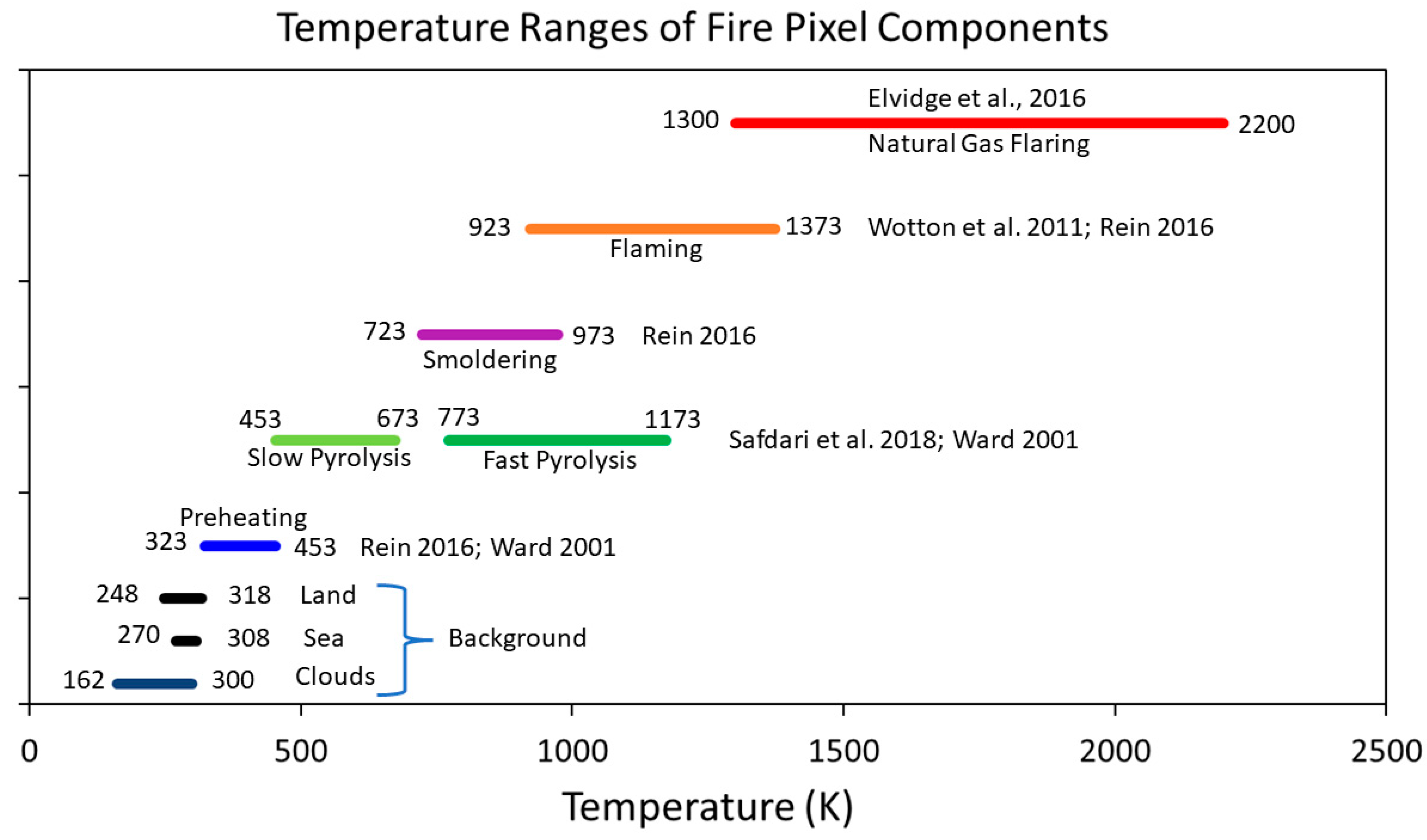
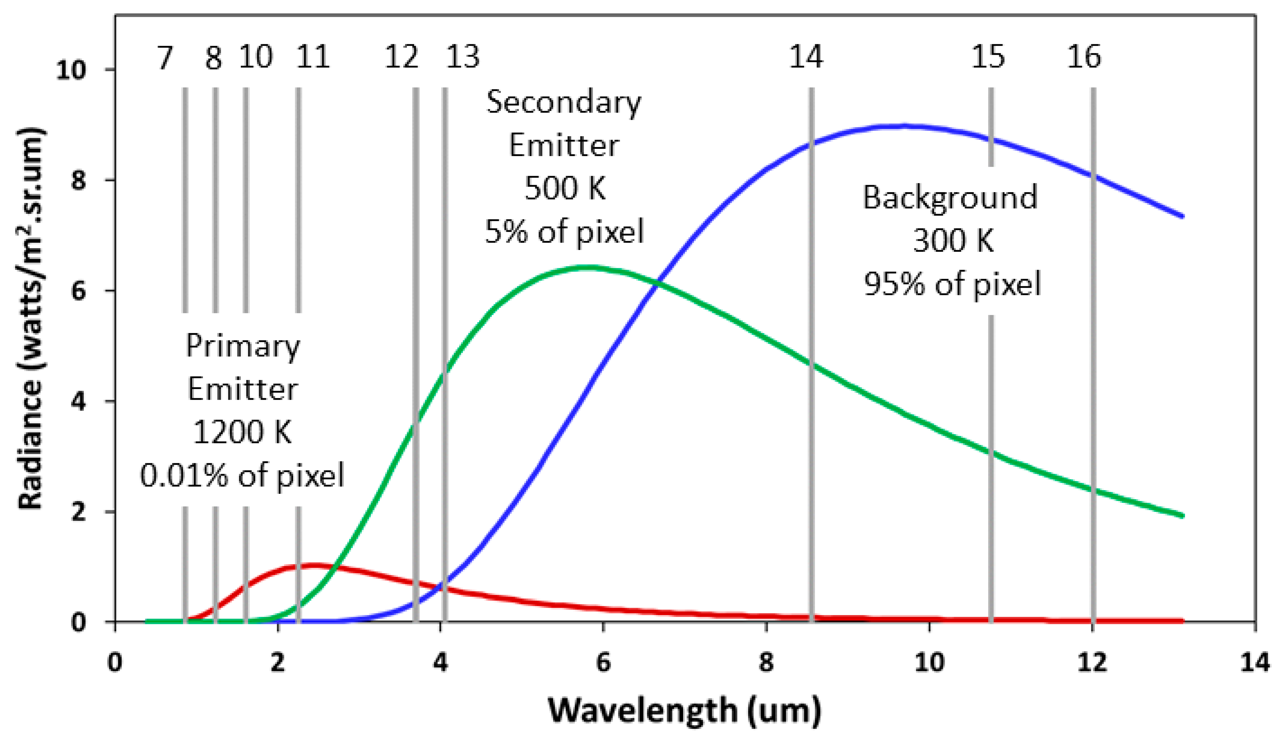
1.2. Temperature Ranges of Fire Pixel Components

Biomass burning is a coupled exothermic/endothermic process that consumes biomass, leaving a mineral ash. The exothermic component is combustion, which produces the heat that drives the endothermic components, which prepares the fuels for combustion. The endothermic phases include preheating and pyrolysis. Preheating drives water from the fuel, preparing it for pyrolysis. In pyrolysis, the structural components of biomass, such as cellulose, hemicellulose and lignin are broken down to volatile gases (pyrolyzate) and char, leaving an ash residue. Char is the fuel of the smoldering phase and pyrolyzate is the fuel of the flaming phase. Flaming is the open air oxidation of volatile gases produced from pyrolysis. Smoldering is the oxidation of the char produced from pyrolysis. Smoldering has a characteristic orange glow present on the char surface. Smoke is the unoxidized fire components that escape to the air [15]. When all the carbon is gone, what remains is mineral ash—primarily oxides of calcium, sodium, and potassium [16]. The basic outlines of pyrolysis, smoldering and flaming are shown in Equations (1)–(3) from Rein, 2016 [17]:
Pyrolysis: Fuel (solid) + Heat => Pyrolyzate (gas) + Char (solid) + Ash (solid)
Smoldering: Char (solid) + O2 (gas) => Heat + CO2 + H2O + Other gases + Ash (solid)
Flaming: Pyrolyzate (gas) + O2 => Heat + CO2 +H2O + Other gases
Figure 4 show the temperature ranges for the basic components that may be present in a VIIRS fire pixel. Background, which normally occupies the largest part of the pixel footprint, includes clouds (162–300 K), sea (270–308 K) and land (248–318 K) [18,19,20]. The temperature ranges of the endothermic components of fire pixels include preheating from 323–453 K [15,16,17], slow pyrolysis from 453–673 K and fast pyrolysis from 773–1173 [15,21]. Smoldering temperatures range from 723–973 K [17]. Flaming biomass ranges from 923–1173 K [17,22]. Natural gas flaring is generally hotter than biomass flaming, with temperatures ranging from 1300–2000 K [23].

1.3. Study Objectives

To date, the flaming subtractive method has only been applied to a single orbit of VIIRS nighttime data, collected over peatland burning in Sumatra. The objective of this study is to evaluate its performance in temperate zone forest fires and natural gas flaring. In addition, because of the large number of misfit pixels found in the Sumatra testing [13], we decided it is important to test additional approaches to the unmixing of primary and secondary emitters from background. In this paper we report on an intercomparison of five methods for subpixel analysis of primary and smoldering combustion in the presence of background using nighttime VIIRS data collected on California mega-fires from 2018 and large natural gas flares present in southern Iraq. In addition, the temperature ranges of the emitters are used to identify the probable fire pixel components responsible for the radiant emissions based on Figure 4.

2. Materials and Methods

We tested and rated five different algorithms for separating primary and secondary emitters in three test sites listed in Table 2. The test sites include the Mendocino and Carr Fires in California plus a set of large natural gas flares in Iraq. Figure 5, Figure 6 and Figure 7 show the set of spectral bands analyzed. Note that in all three test areas the fires and flares show up most clearly in the two SWIR bands. The Mendocino and Carr Fire detections gradually fade and partially disappear moving to either shorter or longer wavelengths. Both the Mendocino and Carr Fires show obvious fire fronts, indicating the fire is spreading outward into unburnt fuels. The Basra gas flares are still clearly present in the NIR bands, but progressively fade as in the LWIR channels.

2.1. VNF Detection Algorithms

VNF uses two types detection algorithms: one for the NIR and SWIR bands (M7, 8, 10, 11) and a second detector for the MWIR (M12–M13). The NIR and SWIR bands are daytime channels, with detection limits and saturation levels set for recording reflected sunlight. At night, they primarily record the noise floor of the system, which is occasionally punctuated by high radiant emissions from fires or flares. Here, we set a detection threshold as the image mean plus four standard deviations. The MWIR signal is a mixture of radiant emissions from clouds, the earth’s surface, and IR emitters. The VNF MWIR thermal anomaly detector relies on the fact that M12 and M13 radiances for background (land, sea, and clouds) are highly correlated, forming a dense diagonal on M12 versus M13 scattergrams (Figure 8). The algorithm generates the MWIR scattergram for a granule or an aggregate, locates the diagonal, and detects pixels with thermal anomalies as outliers pulled away from the diagonal.

2.2. Types of VNF Detections

The VNF pixels are sorted into six types based on the spectral bands having detection.
  • Type 0—Single-band detections. Typically M11 (SWIR). In data collected prior to nighttime M11 collections, it was M10. No Planck curve fitting—no temperature can be calculated.
  • Type 1—NIR and SWIR detection—no MWIR detection. The most common are detections in the two SWIR bands (M10 and M11). Processed with the VNF V.3 dual Planck curve fitting method for a single IR emitter and background.
  • Type 2—M11 and MWIR detection. Processed with the VNF V.3 dual Planck curve fitting method for a single IR emitter and background.
  • Type 3—MWIR only—a rare occurrence. Processed with the VNF V.3 dual Planck curve fitting method for a single IR emitter and background.
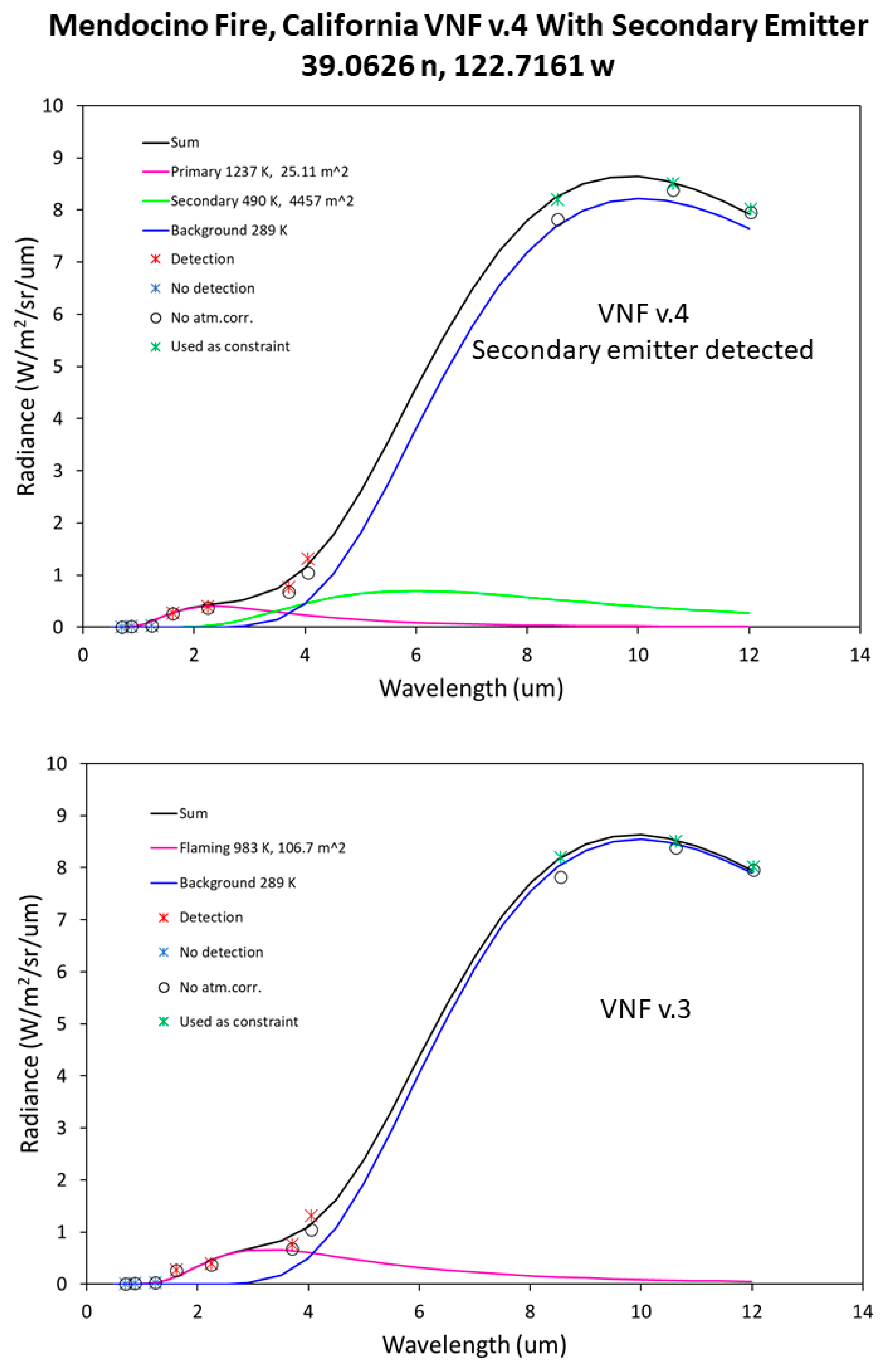
  • Type 4—Has detection in two SWIR bands and MWIR. May have NIR detection as well. The primary and secondary emitter analysis is restricted to Type 4 detections.
  • Type 5—Pixels that yield spurious results revert back to the original dual Planck curve fitting with a single IR emitter plus background.

2.3. Planck Curve Fitting

Planck curve fitting is accomplished using a simplex algorithm [24] to optimize the fit to the radiance data. The fitting starts with initial temperatures of 1000 K for primary emitter, 500 K for the secondary emitter and 300 K for background. The simplex algorithm iteratively modifies the temperature and emission scaling factor (esf) to minimize the residual radiance. The original VNF algorithm uses the fitting procedure to model Planck curves for a single IR emitter phase and a background. This is referred to as “dual-curve” fitting and is applied to the Type 1–3 detections. In the flaming subtractive processing, Type 4 detections are analyzed for three temperature phases: primary and secondary emitters plus the background. These pixels are then filtered to remove those having spurious results, the so called “misfits” (Figure 9). The misfit pixels are converted to Type 5 and are reprocessed with dual Planck curve fitting, solving for a single IR emitter and background.

2.4. Saturation

It is important to exclude radiances affected by saturation in the final Planck curve fitting. The only two spectral bands used in VNF where saturation can be found are M11 and M12 [14]. The general effect of saturation is to reduce the pixel radiance relative to the unaffected bands. Saturation can occur anywhere in the swath. In the nadir aggregation zone three detectors are averaged to make a pixel. Thus, if one of the three is saturated, the result is a radiance less than full-pixel saturation, corrupted by inclusion of a saturated detector radiance. This is also the case for the mid-swath aggregation zone where the signal from two detectors are averaged. Typically, only pixels from the outer aggregation zone reach the saturation radiances. Thus, there are two styles of saturation: “full-pixel saturation” and “subpixel saturation”. Subpixel saturation does not occur in the outer aggregation zone. Full-pixel saturation is unambiguous because the recorded radiance matches the saturation radiances. To identify the presence of subpixel saturation, we look for anomalously low radiances in M11 and M13. For M11, we fit a Planck curve to the M7 –M11 radiances and compared the observed M11 radiance to that predicted from the Planck curve fit. Unsaturated M11 pixels fall on a diagonal in the M11 versus predicted M11 radiance scattergram. Pixels having subpixel M11 saturation are pulled away from the diagonal, with the predicted radiance higher than the observed radiance. For M12 VNF first runs Planck curve fitting using the radiances in all the M bands, reporting out the sum of the squared residuals (SSR). The presence of saturation or other radiance irregularity is indicated by SSR values greater than 2 watts/m2.sr.um. In this case, M11 and M12 are both tested for the presence of subpixel saturation by removing their radiances from Planck curve fitting to check if the SSR drops below 2 watts. The testing is conducted three ways, removal of the M11 radiance, removal of the M12 radiances, and removal of both M11 and M12 radiances. This testing makes it possible to discern whether the subpixel saturation is present in M11, M12, or both spectral bands. The final Planck curve fitting is performed without the spectral bands affected by saturation.

2.5. Atmospheric Correction

An atmospheric correction was developed for the three test areas using Libradtran [25] and applied to the M band radiances of the Type 4 detections. Libradtran was parameterized based on the terrain elevation, atmospheric path length, and atmospheric profiles of water vapor and temperature from simultaneously collected Advanced Technology Microwave Sounder (ATMS) data processed with the Microwave-Integrated Retrieval System (MIRS) [26].
The purpose of atmospheric correction is to derive the surface-emitted radiance Ls from the satellite observed Top-of-Atmosphere (TOA) radiance Lt. The Lt is a measurement of the combined surface-emitted radiance (Ls) and atmospheric up- (Lu) and downwelling (Ld) radiances transmitted through the atmosphere (τ):
Lt = τ⋅(ε⋅Ls + (1 − ε)⋅Ld) + Lu
where ε is the target emissivity, and 1 − ε is the target albedo. To convert Lt to surface temperature, the Lu, Ld, τ, and ε need to be estimated. As suggested in [27], Lu and τ can be determined from Libradtran radiative transfer simulations for ε = 1 at two different surface temperatures Ls1 and Ls2 as the offset and slope of a linear fit of the surface and TOA signals:
τ = (Lt2 − Lt1)/(Ls2 − Ls1)
Lu = Lt1 − τ⋅Ls1
With the knowledge of Lu and τ, Ld can then be computed from the third Libradtran simulation with ε < 1 and Ls = 0:
Ld = Lt − Lu τ (1 − ε)
Ls can then be estimated from Equation (4).

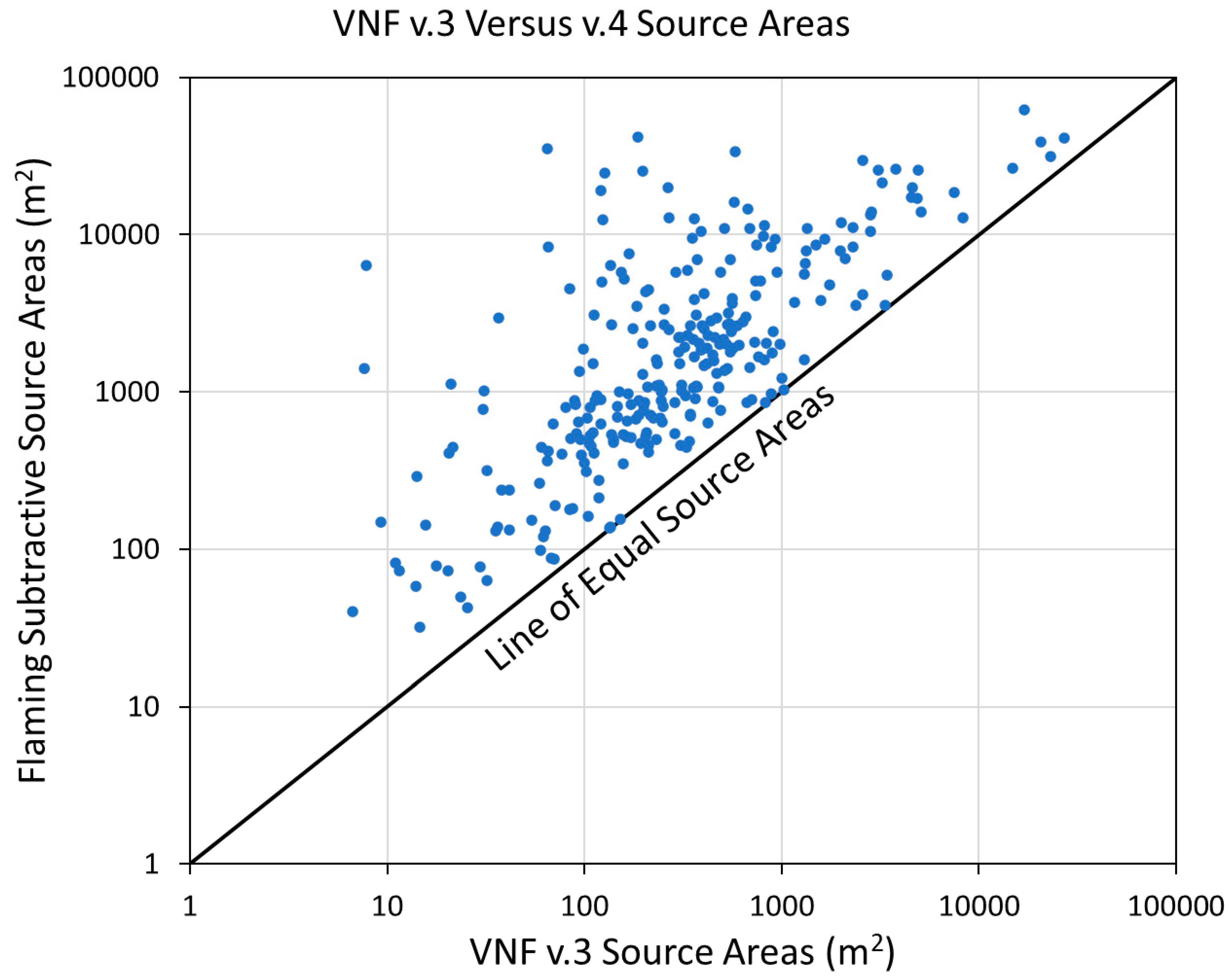
2.6. Flaming Subtractive Method

The NIR and SWIR radiances are used to model the Planck curve of the primary emitter, yielding a temperature, source size and primary emitter radiances in all spectral bands. Residual radiances are calculated based on the subtraction of the primary emitter radiances. Then, dual Planck curve fitting is used to define the secondary emitter and background. The result is a set of temperatures and source areas for three phase: primary emitter, secondary emitter, and background.

2.7. Triple Curve Methods

Simultaneous Planck curve fitting for primary and secondary emitter plus background. Four varieties have been tested:
  • Unconstrained—observed radiances only.
  • Constrained by the primary emitter temperature calculated from Planck curve fitting of the NIR and SWIR detection radiances.
  • Constrained by the local background temperature.
  • Constrained by the primary emitter temperature and local background temperature.

2.8. Rating

The five methods were rated based on the number of “misfit” detections. Misfits are recognized based on implausible results. Examples include unrealistically low secondary emitter or background temperatures (Figure 9). Results from each of the tested methods were inspected and criteria were developed to filter out misfits. Since the same set of Type 4 pixels were processed in each method, the number of misfits found can be used to rate the methods. The rating is in the form of percent yield.

3. Results

3.1. Scoring the Methods

Table 3 shows the scoring of the five methods, listing misfit tallies by type and the yield calculation. The yield is calculated as the percentage of the Type 4 detections that yield valid secondary emitter results. As with previous tests conducted on a Sumatra peatland fire, the flaming subtractive algorithm has the highest yield. The rest of this paper focuses on exploring the flaming subtractive results.

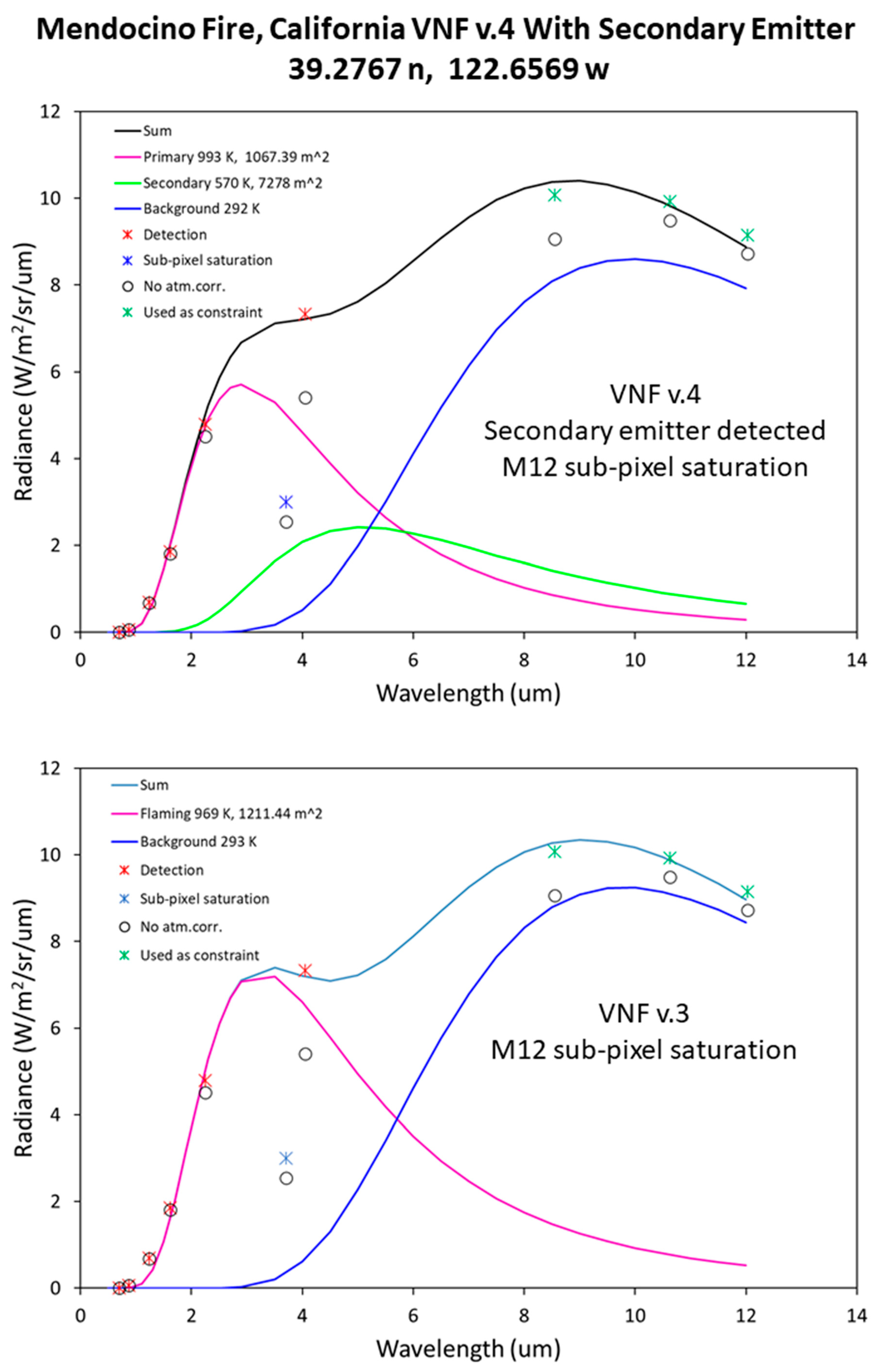
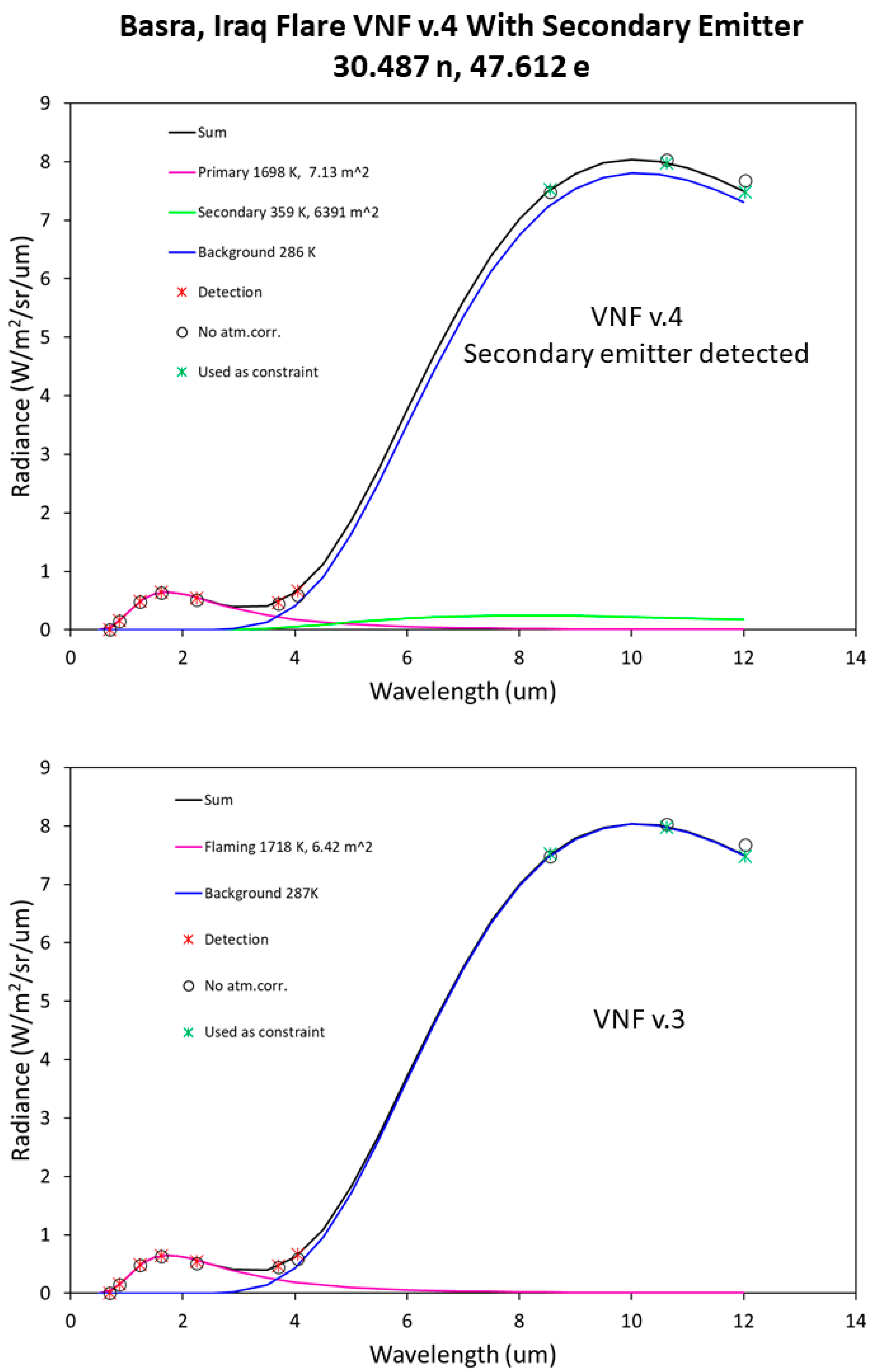
3.2. Examples of Good Fits

Figure 10, Figure 11 and Figure 12 shows three examples of good fits, side by side with the VNF V.3 results for the same pixels. Figure 10 and Figure 11 are from the Mendocino Fire and Figure 12 is from a Basra gas flare.
In Figure 10, VNF V.3 the IR emitter, calculated from the NIR, SWIR and MWIR radiances came out with a temperature of 894 K and area of 211 m2. The flaming subtractive method successfully split the fire radiant energy into primary and secondary IR emitters. Using the NIR and SWIR radiances to model the Planck curve of the primary emitter results in a slightly hotter and smaller source size, with a temperature of 1237 K and 25 m2. The secondary emitter, calculated from the residual radiances after subtracting the flaming phase, has a temperature of 490 K and source size of 4458 m2.
Figure 11 shows a Mendocino Fire pixel with much higher radiances in the spectral bands. In fact, M12 has subpixel saturation and has been excluded from Planck curve fitting in both V.3 and V.4. The V. 3 processing resulted in a primary emitter temperature of 894 K and source size of 2297 m2. Splitting the radiant emissions with the flaming subtractive methods results in a primary emitter at 993 K and 1067 m2 plus a secondary emitter at 570 K and 7278 m2.
Figure 12 shows a gas flare detection from Basra. The V.3 algorithm calculated the IR emitter temperature as 1690 K and source size of 7.65 m2. By modeling the primary emitter with the NIR and SWIR radiances the temperature rises slightly to 1704 K and source size drops slightly to 7.26 m2. The dual Planck curve fitting on the residual radiances found a secondary emitter at 399 K and 1400 m2.

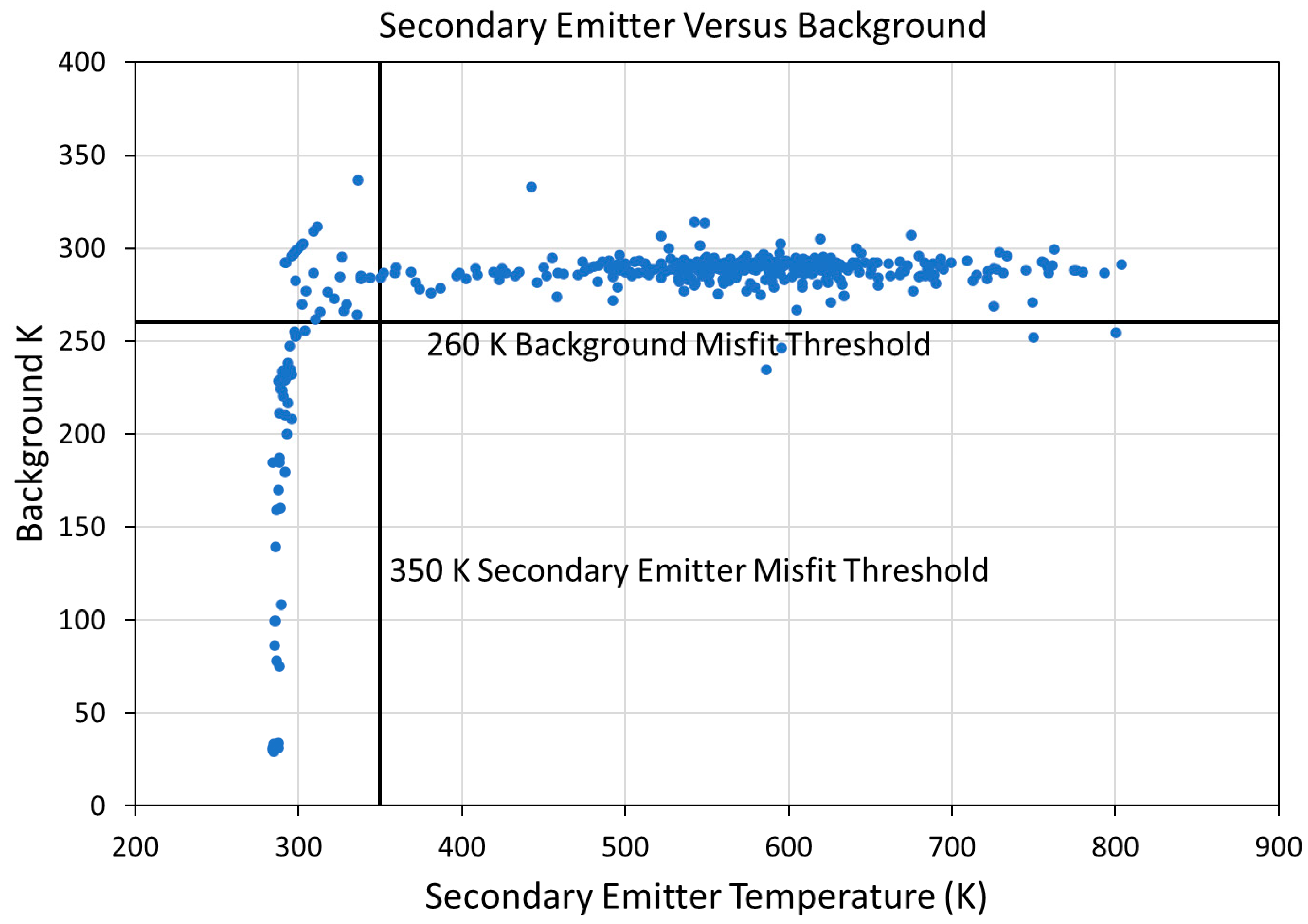
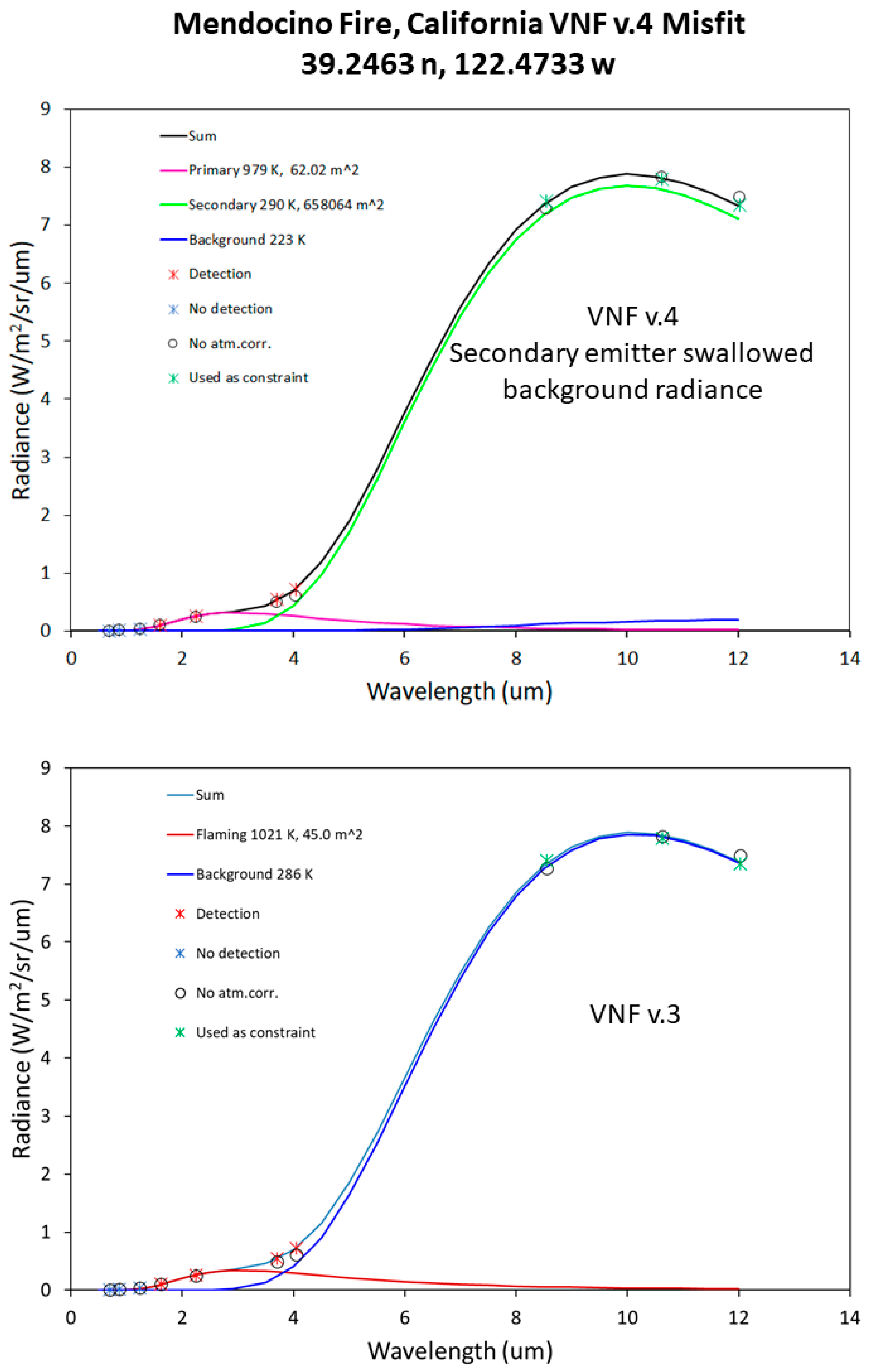
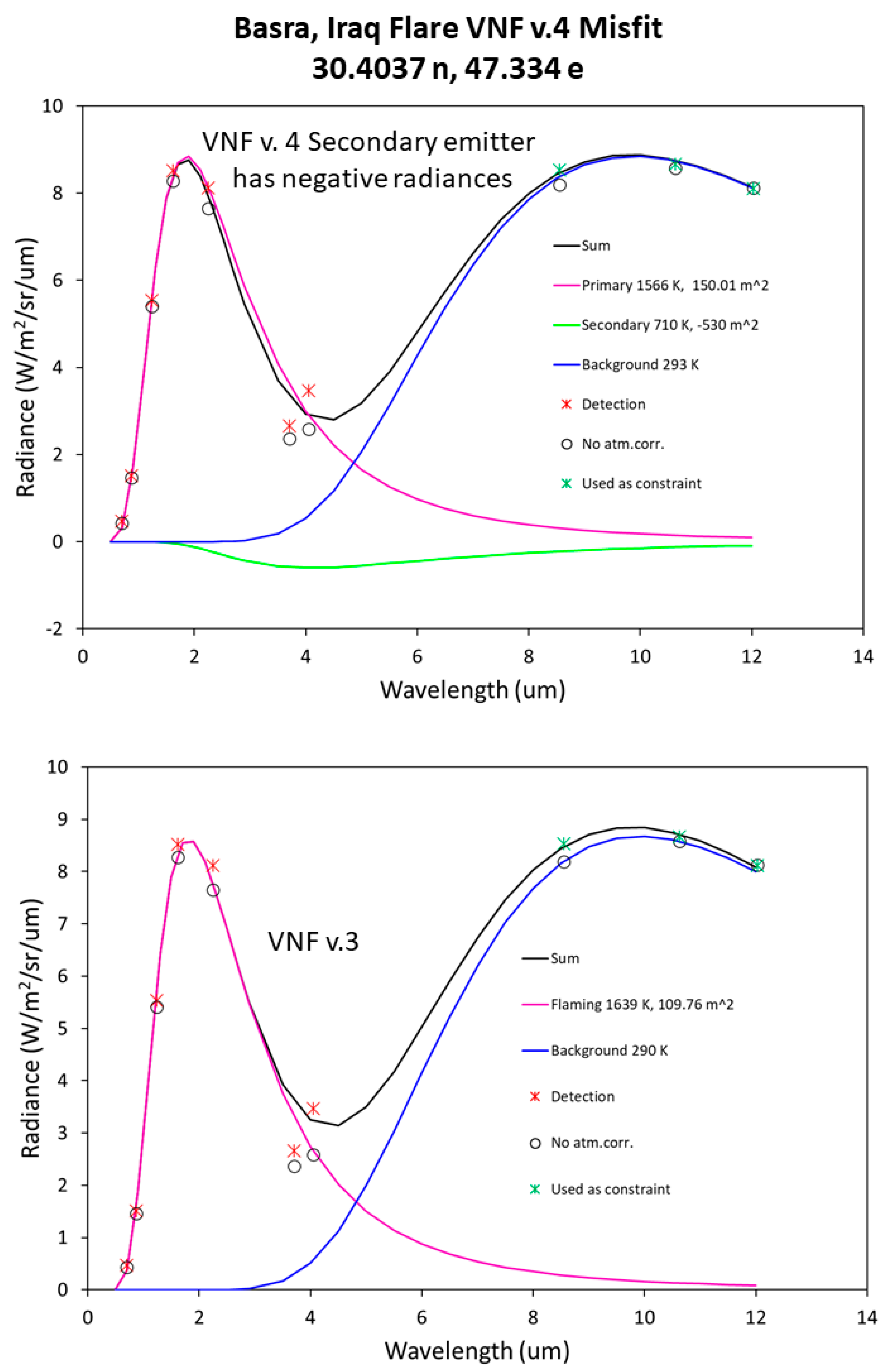
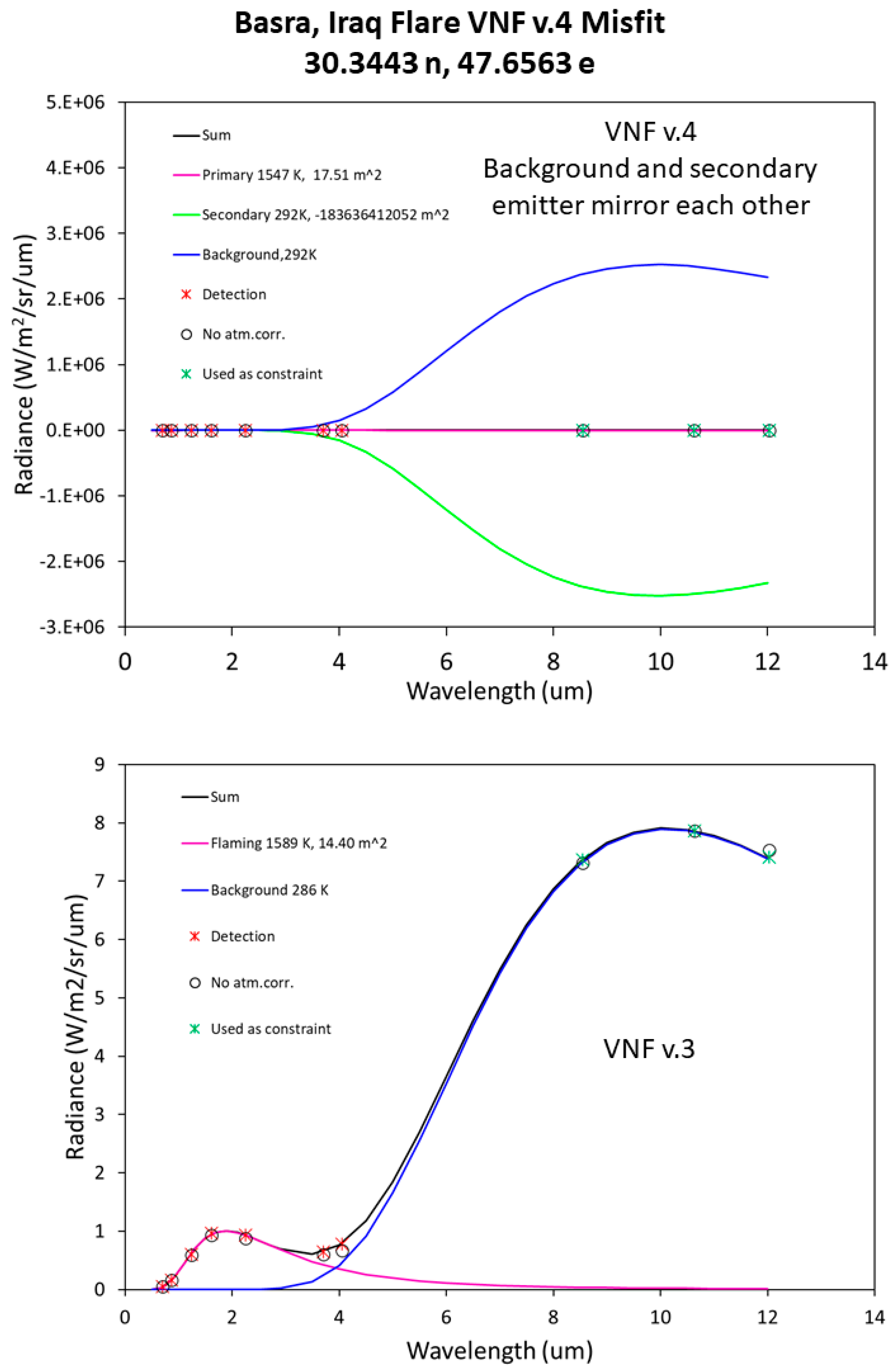
3.3. Examples of Misfits

Figure 13, Figure 14 and Figure 15 shows three examples of misfits, side by side with the VNF V.3 results for the same pixels. The misfit pixels revert to V.3 processing since the flaming subtractive method produced spurious results.
Figure 13, from the Mendocino Fire, shows a common type of misfit, in which the secondary emitter Planck curve has absorbed a large portion of the background radiance. The V.3 processing yielded an IR emitter at 945 K with a source area of 80 m2. The flaming subtractive method resulted in a primary emitter temperature of 979 K and source area of 62 m2—slightly hotter and smaller than V.3. The misfit classification comes from the secondary emitter, which came out at 290 K and source area of 658,064 m2. This pushed the background temperature down to 223 K—an unrealistic value given the clear sky conditions. This style of misfit can be traced to the extremely high secondary emitter esf. This pulls the secondary emitter temperature down to the background level and the source size expands to nearly the full pixel footprint.
Figure 14, from a Basra flare, shows the other common type of misfit, traced to a negative esf for the secondary emitter. From V.3 the IR emitter temperature 1604 K and source area is 129 m2. When the flaming subtractive method is applied the primary emitter comes out as 1566 K and 150 m2. The pixel is classified as a misfit because the secondary emitter’s esf is negative, resulting in a source area of −530 m2.
Another example of a VNF v.4 misfit is shown in Figure 14. Here, the secondary emitter’s esf is highly negative, resulting in the background and secondary emitter’s Planck curves forming mirror images of each other—both with temperatures of 292 K.

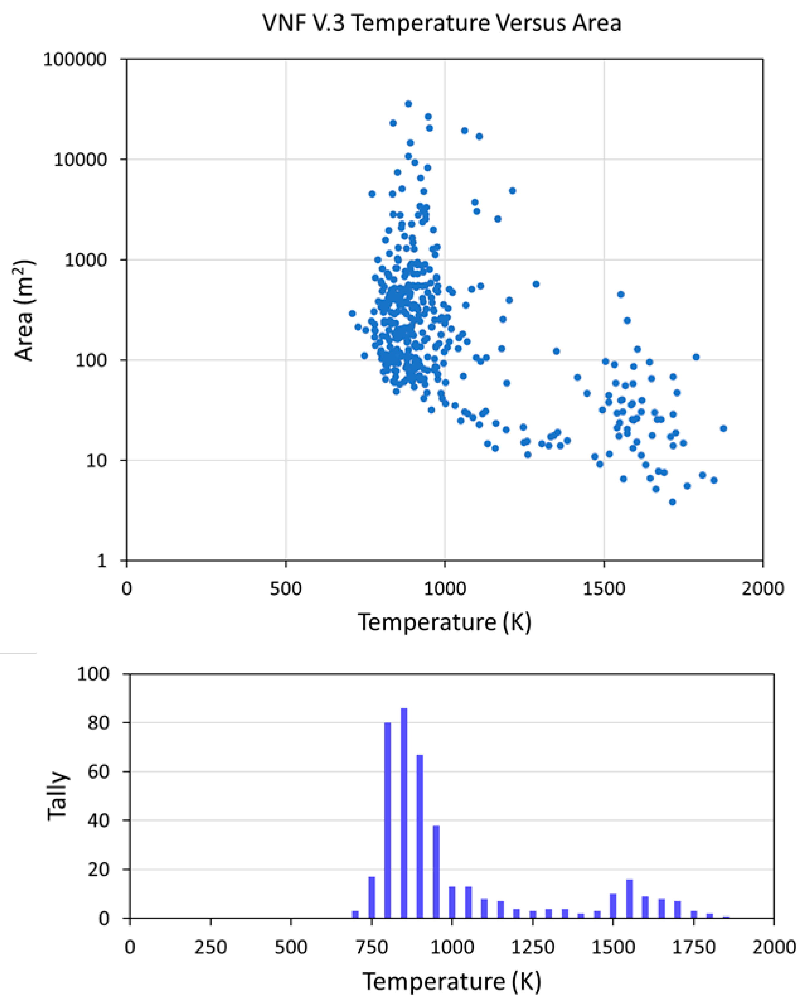
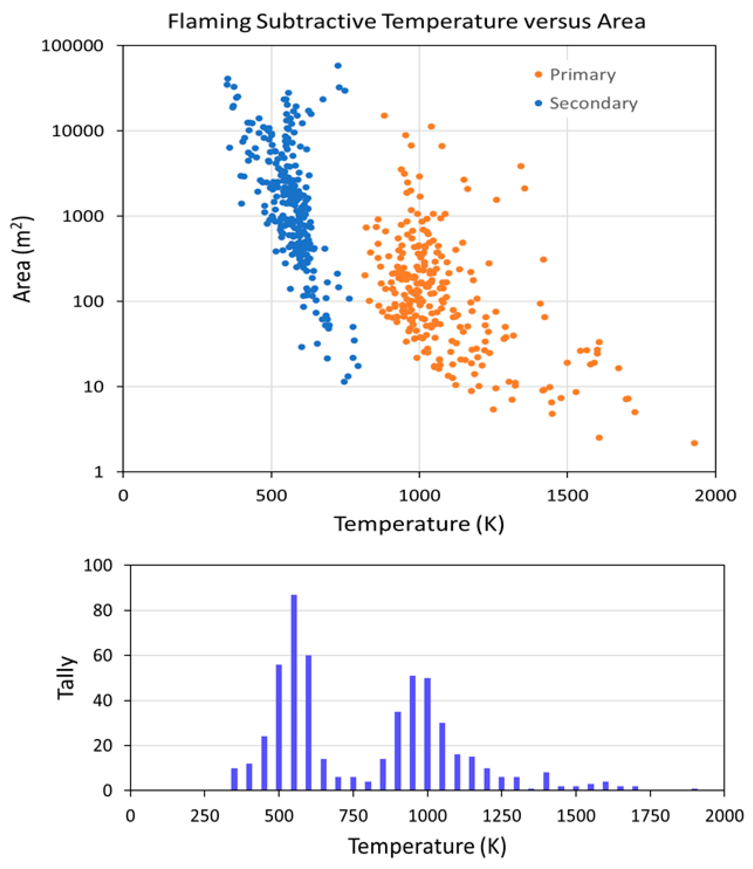
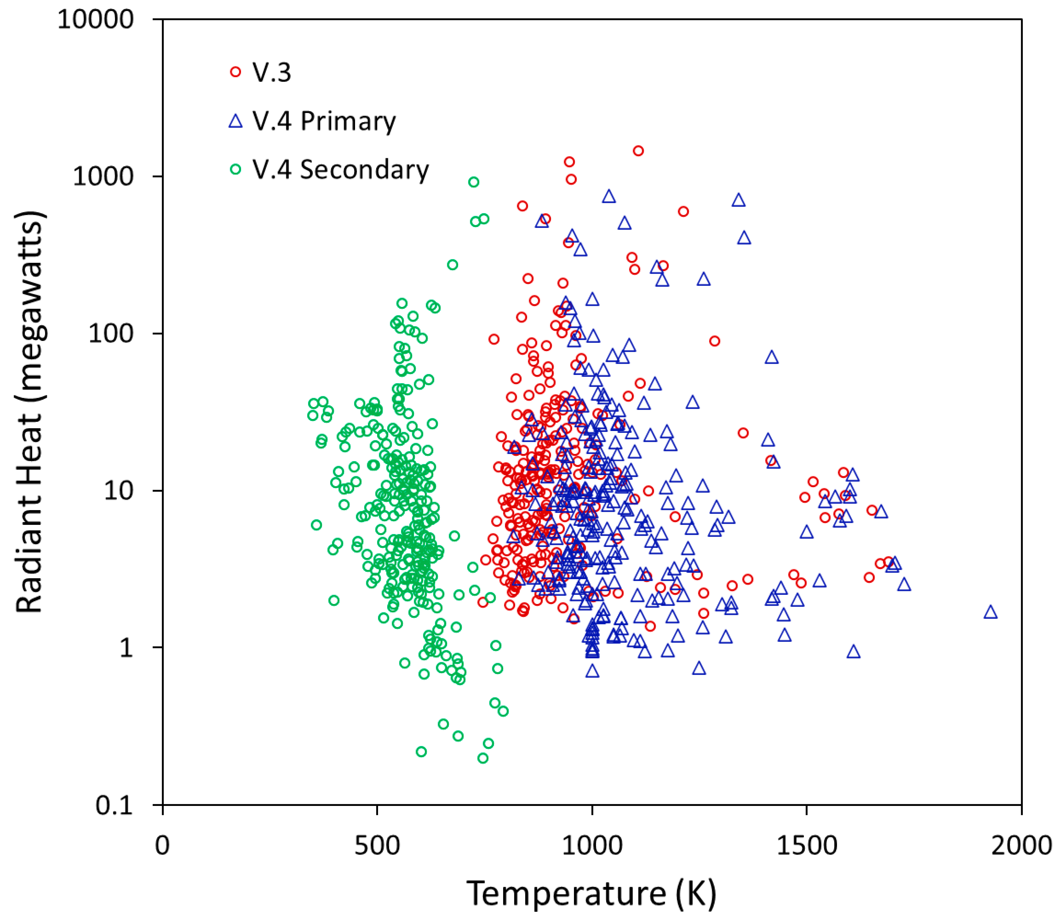
3.4. Temperature versus Source Area Scattergrams and Temperature Histograms

The original VNF (v.3) performs dual Planck curve fitting on radiances spanning NIR to LWIR, calculating a single subpixel infrared emitter temperature and source size in the presence of a cool background (clouds and earth surfaces). In this case, the IR emitter temperatures and source areas are dominated by the flaming phase due to the T4 term in the Stefan–Boltzmann Law. Figure 16 shows the VNF v.3 scattergram of temperatures and source areas, plus the corresponding temperature histogram. VNF v.3 produces a bimodal distribution—with a hot peak associated with natural gas flares near 1600 K and a peak centered near 900 K arising primarily from biomass burning.
The flaming subtractive method splits a pixel’s multispectral radiances into three phases—primary emitter, secondary emitter and background. This is accomplished by fitting a Planck curve to the NIR and SWIR radiances to represent the primary emitter. The primary emitter radiances are calculated in each spectral band from the primary emitter Planck curve and are subtracted from the original radiances. Then, dual Planck curve fitting is applied to the residual radiances to derive a secondary emitter phase and background.
Figure 17 shows the temperature versus area scattergram and temperature histogram from the flaming subtractive method. Only the pixels having “fits” are shown. The prominent v.3 peak near 900 K is split into a cooler peak near 550 K and warmer peak near 1000 K. The gas flaring peak near 1600 K is diminished by the low number of gas flaring detections found to have a valid secondary emitter fits.

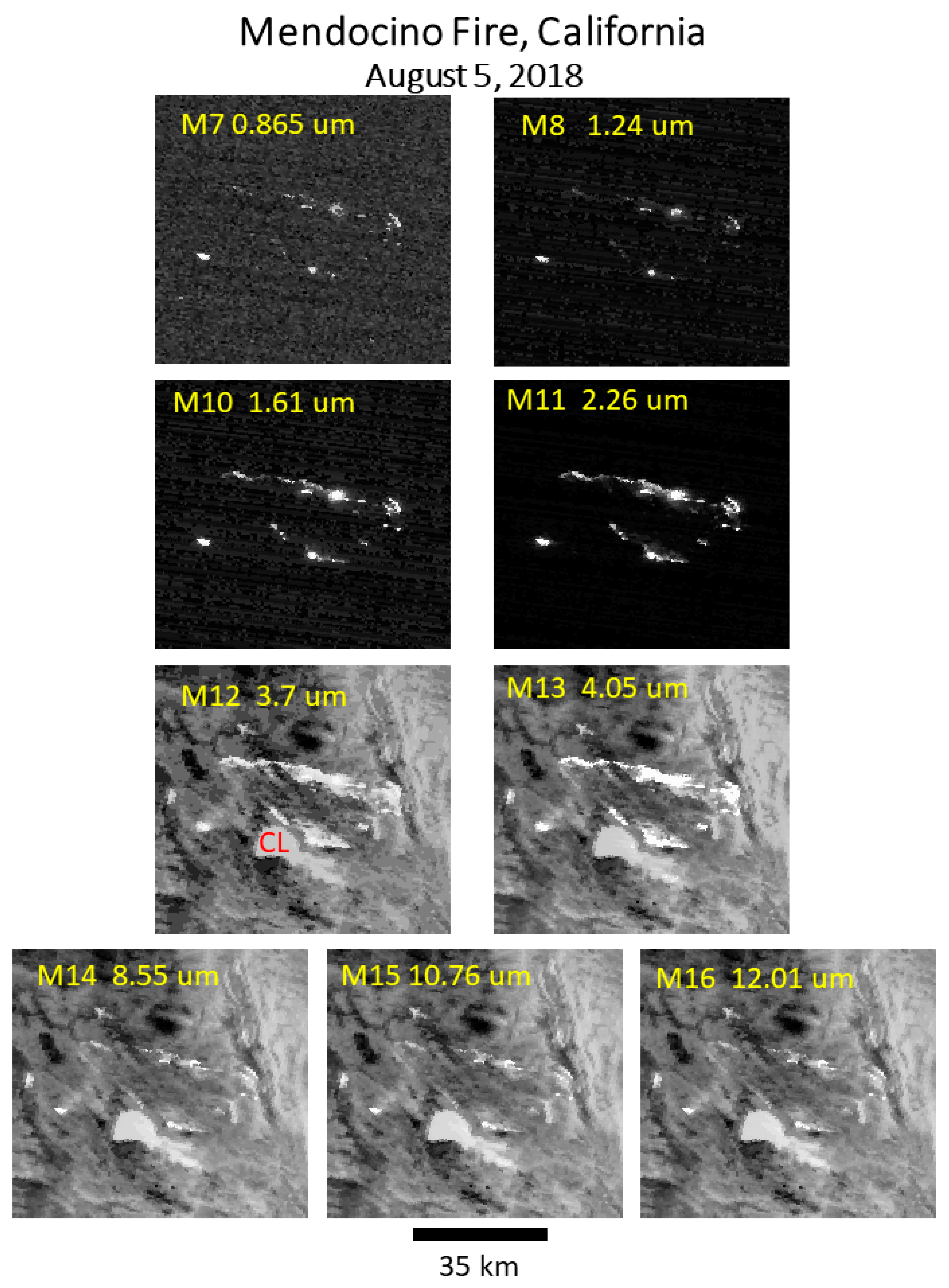
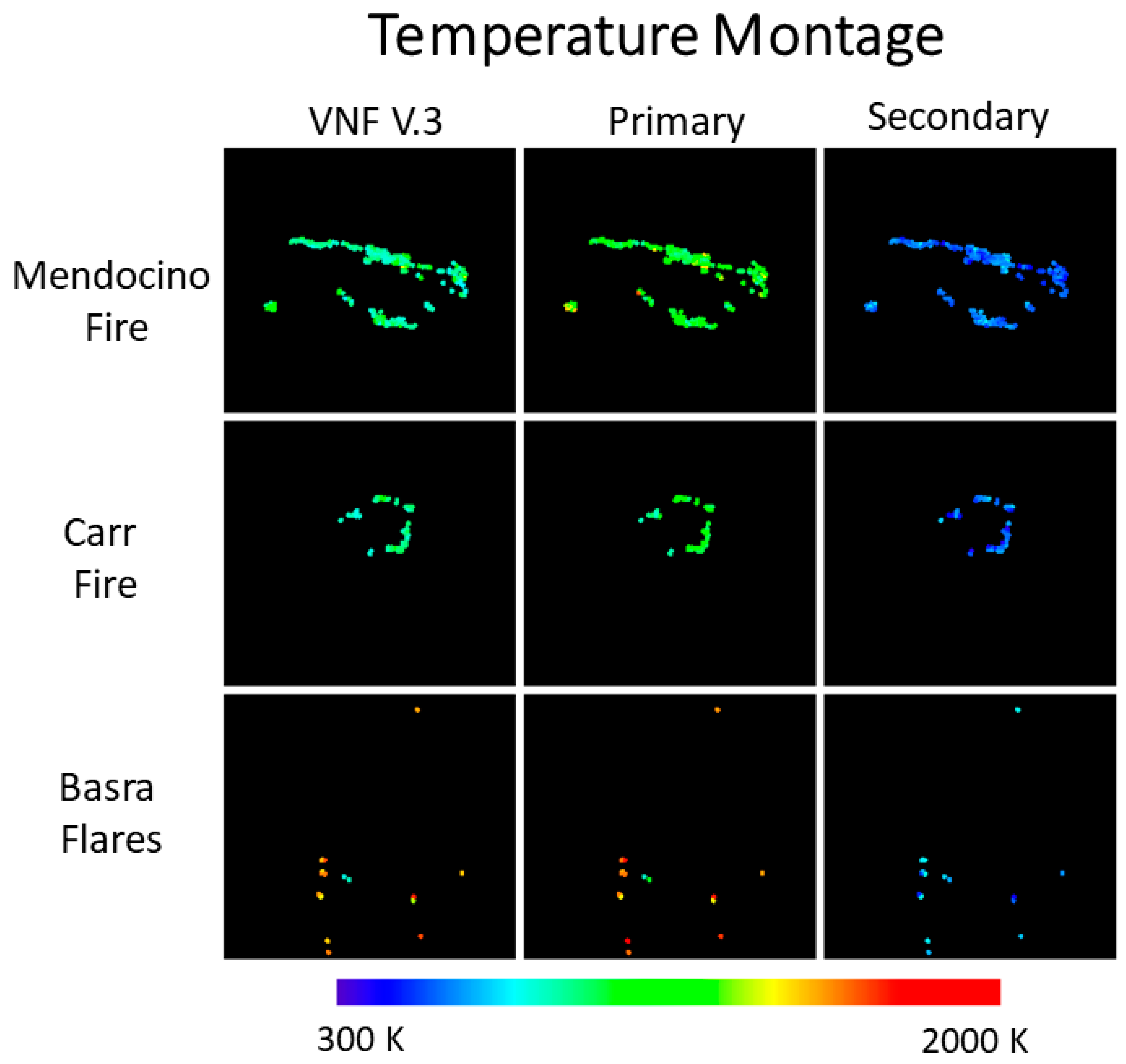
3.5. Temperature Montage

Figure 18 shows a temperature montage of the VNF Type 4 detections from the three test sites. The VNF v.3 temperature images are on the left side. In the middle are the primary emitter temperature images and on the right are the secondary emitter temperature images. Note that flaming subtractive procedure raises the temperatures of the primary emitter slightly relative to v.3. In contrast, the secondary emitter temperatures are generally 400–500 K cooler than the v.3 temperatures for the same pixel.

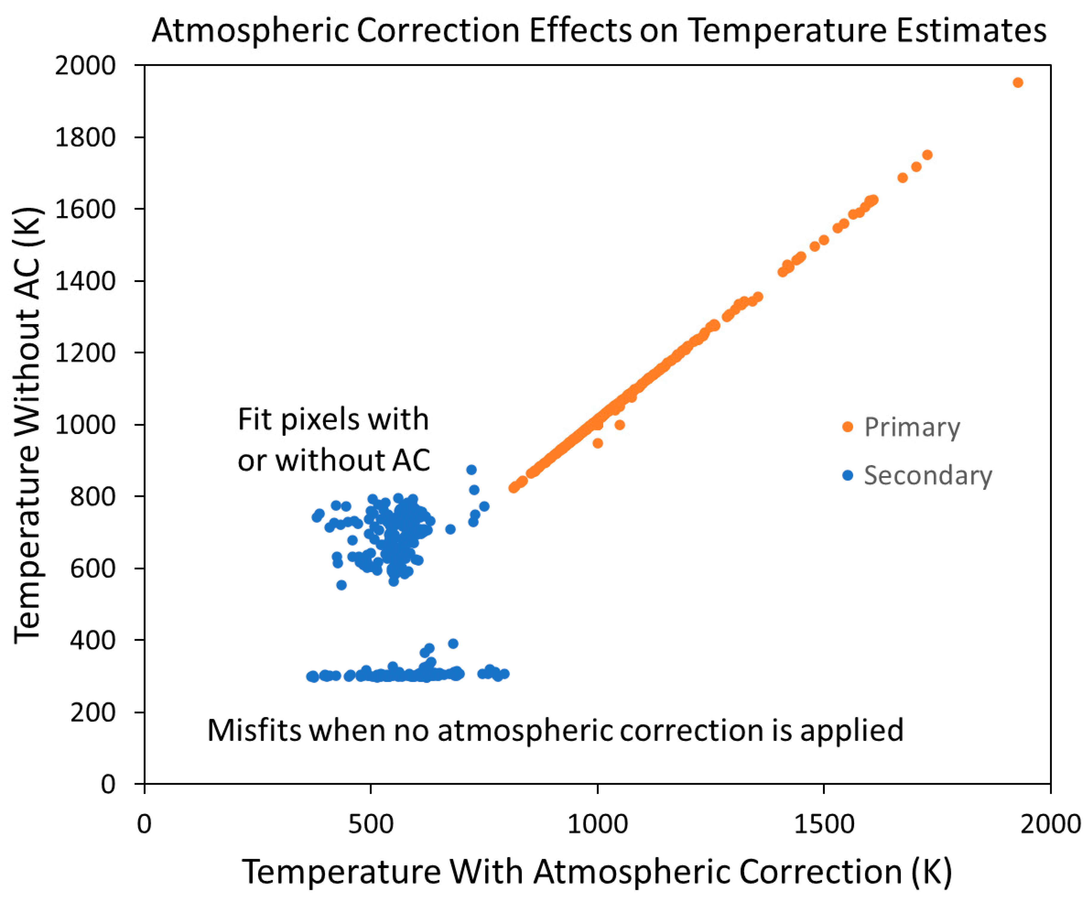
3.6. Atmospheric Correction Effect

Figure 19 is a scattergram of the flaming subtractive derived temperatures with and without atmospheric correction. The atmospheric correction had little influence on the primary emitter temperatures. We believe this is attributable to high atmospheric transmissivity in the VIIRS SWIR spectral bands, the dry atmospheres of the test sites, and near nadir location of fires, which minimizes variation in atmospheric path length. Significantly, the atmospheric correction doubled the number of secondary emitter fits and shifted the temperatures to form a histogram peak at 550 K.

4. Discussions

The VNF v.3 temperatures, source areas, and radiant heat are dominated by the high temperature exogenic combustion components. This is the case because the exogenic components are substantially hotter than the endothermic components. The exothermic component’s dominance of the v.3 product can be attribute to the exponential rise in radiant emissions due to the T4 term in the Stefan–Boltzmann Law. The high degree of similarity between the VNF v.3 data and the primary emitter from the flaming subtractive analysis can be seen in Figure 20, which shows temperatures and radiant heat for the Type 4 pixels from the study set. Using the short wavelength radiances to model the primary emitter Planck curve results in a slight increase in temperature and a slight decrease in source size as compared to the v.3 results.
Regarding the identity of the primary and secondary emitter components, let us examine the temperature ranges of the phases relative to the temperature ranges for fire pixel components shown in Figure 4. The biomass burning primary emitter peaks at 950 K, but spans 800–1300 K (Figure 17). This corresponds to the flaming phase, with possible contribution from smoldering and fast pyrolysis. The secondary emitter peaks at 550 K and spans 350–750 K, corresponding to the preheating and slow pyrolysis components.
In the two biomass burn test cases (Mendocino and Carr), the secondary emitter is linked to the radiant emissions from the endothermic portion of the biomass burning system. The preheating and slow-pyrolysis radiant emissions are hidden under the higher radiant output of the exothermic components. Subtraction of the primary emitter radiances makes it possible uncover the presence of the secondary emitter, which then can be split from the background radiance through dual Planck curve fitting. The flaming subtractive processing result is a substantial increase in the total radiant heat (Figure 20) and total source area (Figure 21).
Looking at Figure 5, Figure 6 and Figure 7, one might conclude that full pixels are on fire. However, amongst this test set, none of the VNF pixel emission scaling factor’s (esf) rose above 0.1 or 10% of the pixel footprints (Figure 22).

5. Conclusions

We have developed a flaming subtractive method for subpixel unmixing of radiant emissions from two IR emitter temperature phases present in fire pixels at night. The primary emitter temperature and source area are calculated using the Planck curve defined based on the NIR and SWIR radiances. The primary emitters Planck curve is used to calculate primary emitter radiances in all spectral bands, which are subtracted to create residual radiances. The residual radiances are analyzed for a secondary IR emitter and a cool background. Spurious secondary emitter results are filtered out based on unrealistic esf, temperature and source area values. The failure of the fitting indicates that a secondary emitter could not be found. These “misfit” pixels revert back to the dual-curve fitting for a single IR emitter and background—the standard processing from VNF v.3. The flaming subtractive analysis is the key addition to VNF version 4.
We have now applied the split IR emitter analysis to both nighttime Landsat and nighttime VIIRS data in a total of five test sites. The Landsat analysis used the “tip and tail” method to model the primary emitter Planck curve with NIR and SWIR radiances and the secondary emitter Planck curve is derived from the LWIR radiances. The “tip and tail” method makes no attempt to separate secondary emitter and background radiant emissions. The flaming subtractive method explicitly attempts to unmix temperatures and source areas for three temperature phases present in fire pixels: primary emitter, secondary emitter and background. The flaming subtractive analysis makes use of nighttime VIIRS data collected from nine spectral bands in four spectral ranges: NIR, SWIR, MWIR and LWIR.
The temperature of the secondary emitter has varied between the five test sites. In the Landsat 8 study of a smoldering peatland fires, the secondary emitter temperature was 320–450 K, indicating pre-heating. This is the result of smoldering in the soil column heating the soil surface. In the VIIRS analysis of a smoldering peatland fire in Sumatra, two secondary emitter temperature ranges emerged—one from preheating (320–450 K) and one from pyrolysis/smoldering from 650 to 750 K. In the 2018 California megafires, the secondary emitter had temperatures from 350 to 650 K, covering the temperature ranges typical of pre-heating and slow pyrolysis. Several of the gas flares in Basra had 2nd phases but the temperatures were highly variable, spanning 350–800 K. The identity of the secondary emitter found at gas flaring sites will require further investigation.
Our results indicate that an atmospheric correction is quite important for the flaming subtractive analysis. The atmospheric correction had minimal impact on the flaming-phase analysis in these three test cases. This may be due to high transmissivity in the SWIR spectral bands in the dry atmospheres present in Northern California and Southern Iraq. However, adding the atmospheric corrected resulted in a doubling in the number of good 2nd-phase fits. In addition, inclusion of an atmospheric correction results in a ~150 K decline in the 2nd-phase temperature.
Our plan is to implement global near-real-time processing with the flaming subtractive algorithm as VNF version 4 for both VIIRS instruments (SNPP and NOAA-20). Production of the VNF v.3 product will continue. Later we plan to reprocess the VIIRS archive to extend VNF v.4 record back to the beginning of the VIIRS archive. The M11 collections extend back to the beginning of 2018. The algorithm can still work if there is detection in at least two of the three short wavelength channels (M7, M8 and M10) collected in the first five years of VIIRS data. This will cut the number of VNF detections that can be processed with the VNF v. 4 algorithm from 2012 through 2017.
By splitting the primary and secondary emitters apart, there is an approximate doubling of the VNF calculated source area and radiant heat. It will be important to examine the validity of VNF v.4 primary and secondary emitter results using independent data sources. This could include maps of flaming fire fronts and smoldering combustion made by firefighters, airborne multispectral data collected on active fires, and nighttime Landsat, which has many of the same set of spectral bands as VIIRS, though missing the MWIR bands.
The capability to distinguish multiple components of biomass burning from space has the potential to improve the identification of core zones having the largest mass of combustion biomass during fire suppression efforts, modeling of smoke production, the proportion of partially oxidized greenhouse gas emissions, and the severity of the burning. While there are several factors that affect the proportion of the components, fuel size is a major determining factor. Flaming predominates in grassland fires, where the fuels have large surface areas and are readily combusted [28]. Forest fires tend to start with flaming-phase combustion in fine dry fuels, such as beds of dry pine needles. Heat from the flaming combustion eventually induces pyrolysis and combustion of larger wood branches and trunks. The standard satellite hotspot is unable to distinguish multiple temperature phases present in biomass burning. However, this can be accomplished at night if there are multiple spectral bands that span a wide range of wavelengths.

Author Contributions

Conceptualization and writing, C.D.E.; algorithm development and processing, M.Z.; preparation of figures, F.C.H. and T.G.; manuscript editing, T.S. All authors have read and agreed to the published version of the manuscript.

Funding

The original VIIRS Nightfire algorithm development was funded 2012-2015 by the NOAA Joint Polar Satellite System (JPSS) proving ground program. The research on dual temperature extraction was initiated using nighttime Landsat data in a project conducted in Indonesia funded by the U.S. Forest Service (USFS) international program office. The research continued from 2016 to 2018 funded by NASA’s Carbon Monitoring System. The development of a VIIRS algorithm for dual IR emitter analysis has been funded by the NOAA JPSS provind ground program. The final year of the effort was funded by NOAA JPSS through a subcontract from the Cooperative Institute for Research on Atmosphere at the Colorado State University. Additional support for this study was provided by the Oil and Gas Climate Initiative.

Informed Consent Statement

Not applicable.

Data Availability Statement

The nightly VNF v.3 data are available at https://eogdata.mines.edu/products/vnf/, accessed on 31 October 2021.

Acknowledgments

The authors gratefully acknowledge NOAA for providing access to the nightly global VIIRS data used in this study.

Conflicts of Interest

The authors declare no conflict of interest.

References

  1. Planck, M. The Theory of Heat Radiation, 2nd ed.; Masius, M., Translator; P. Blakiston’s Son & Co.: Philadelphia, PA, USA, 1914. [Google Scholar]
  2. Weinreb, M.P.; Hill, M.L. Calculation of Atmospheric Radiances and Brightness Temperatures: In infrared Window Channels of Satellite Radiometers; No. 80; US Department of Commerce, National Oceanic and Atmospheric Administration, National Environmental Satellite Service: Washington, DC, USA, 1980.
  3. Planck, M. On the law of distribution of energy in the normal spectrum. Ann. Phys. 1901, 4, 553. [Google Scholar] [CrossRef]
  4. Planck, M. The theory of heat radiation. Entropie 1900, 144, 164. [Google Scholar]
  5. Dozier, J. A method for satellite identification of surface temperature fields of sub-pixel resolution. Remote Sens. Environ. 1981, 11, 221–229. [Google Scholar] [CrossRef]
  6. Elvidge, C.D.; Zhizhin, M.; Hsu, F.-C.; Baugh, K.E. VIIRS nightfire: Satellite pyrometry at night. Remote Sens. 2013, 5, 4423–4449. [Google Scholar] [CrossRef] [Green Version]
  7. Lee, T.F.; Tag, P.M. Improved detection of hotspots using the AVHRR 3.7-um channel. Bull. Am. Meteorol. Soc. 1990, 71, 1722–1730. [Google Scholar] [CrossRef] [Green Version]
  8. Justice, C.; Giglio, L.; Korontzi, S.; Owens, J.; Morisette, J.; Roy, D.; Descloitres, J.; Alleaume, S.; Petitcolin, F.; Kaufman, Y. The MODIS fire products. Remote Sens. Environ. 2002, 83, 244–262. [Google Scholar] [CrossRef]
  9. Li, F.; Zhang, X.; Kondragunta, S.; Csiszar, I. Comparison of fire radiative power estimates from VIIRS and MODIS observations. J. Geophys. Res. Atmos. 2018, 123, 4545–4563. [Google Scholar] [CrossRef]
  10. Wooster, M.J.; Roberts, G.; Perry, G.; Kaufman, Y.J. Retrieval of biomass combustion rates and totals from fire radiative power observations: FRP derivation and calibration relationships between biomass consumption and fire radiative energy release. J. Geophys. Res. Atmos. 2005, 110, 24. [Google Scholar] [CrossRef]
  11. Fisher, D.; Wooster, M.J. Shortwave IR adaption of the mid-infrared radiance method of fire radiative power (FRP) retrieval for assessing industrial gas flaring output. Remote Sens. 2018, 10, 305. [Google Scholar] [CrossRef] [Green Version]
  12. Elvidge, C.D.; Zhizhin, M.; Hsu, F.-C.; Baugh, K.; Khomarudin, M.R.; Vetrita, Y.; Sofan, P.; Hilman, D. Long-wave infrared identification of smoldering peat fires in Indonesia with nighttime Landsat data. Environ. Res. Lett. 2015, 10, 065002. [Google Scholar] [CrossRef] [Green Version]
  13. Elvidge, C.D.; Zhizhin, M.; Baugh, K.; Hsu, F.-C. Identification of Smoldering Peatland Fires in Indonesia via Triple-Phase Temperature Analysis of VIIRS Nighttime Data. In Biomass Burning in South and Southeast Asia; CRC Press: Boca Raton, FL, USA, 2021; pp. 25–38. [Google Scholar]
  14. Elvidge, C.D.; Zhizhin, M.; Baugh, K.; Hsu, F.-C.; Ghosh, T. Extending Nighttime Combustion Source Detection Limits with Short Wavelength VIIRS Data. Remote Sens. 2019, 11, 395. [Google Scholar] [CrossRef] [Green Version]
  15. Ward, D. Combustion chemistry and smoke. In Forest Fires; Academic Press: Cambridge, MA, USA, 2001; pp. 55–77. [Google Scholar]
  16. Bodí, M.B.; Martin, D.A.; Balfour, V.N.; Santín, C.; Doerr, S.H.; Pereira, P.; Cerdà, A.; Mataix-Solera, J. Wildland fire ash: Production, composition and eco-hydro-geomorphic effects. Earth-Sci. Rev. 2014, 130, 103–127. [Google Scholar] [CrossRef]
  17. Rein, G. Smoldering Combustion, Chapter 19. In SFPE Handbook of Fire Protection Engineering, 5th ed.; Springer: Berlin/Heidelberg, Germany, 2016; pp. 581–603. Available online: http://link.springer.com/chapter/10.1007/978-1-4939-2565-0_19 (accessed on 31 October 2021).
  18. Stubenrauch, C.J.; Rossow, W.B.; Kinne, S.; Ackerman, S.; Cesana, G.; Chepfer, H.; Di Girolamo, L.; Getzewich, B.; Guignard, A.; Heidinger, A.; et al. Assessment of global cloud datasets from satellites: Project and database initiated by the GEWEX radiation panel. Bull. Am. Meteorol. Soc. 2013, 94, 1031–1049. [Google Scholar] [CrossRef]
  19. Webb, P. Introduction to Oceanography; Roger Williams University Pressbooks: Bristol, RI, USA, 2019. [Google Scholar]
  20. Wan, Z.; Zhang, Y.; Zhang, Q.; Li, Z.-L. Quality assessment and validation of the MODIS global land surface temperature. Int. J. Remote Sens. 2004, 25, 261–274. [Google Scholar] [CrossRef]
  21. Safdari, M.S.; Rahmati, M.; Amini, E.; Howarth, J.E.; Berryhill, J.P.; Dietenberger, M.; Weise, D.R.; Fletcher, T.H. Characterization of pyrolysis products from fast pyrolysis of live and dead vegetation native to the Southern United States. Fuel 2018, 229, 151–166. [Google Scholar] [CrossRef]
  22. Wotton, B.M.; Gould, J.S.; McCaw, W.L.; Cheney, N.P.; Taylor, S.W. Flame temperature and residence time of fires in dry eucalypt forest. Int. J. Wildland Fire 2011, 21, 270–281. [Google Scholar] [CrossRef]
  23. Elvidge, C.D.; Zhizhin, M.; Baugh, K.; Hsu, F.-C.; Ghosh, T. Methods for global survey of natural gas flaring from visible infrared imaging radiometer suite data. Energies 2016, 9, 14. [Google Scholar] [CrossRef]
  24. Lagarias, J.C.; Reeds, J.A.; Wright, M.H.; Wright, P.E. Convergence properties of the Nelder-Mead simplex method in low dimensions. SIAM J. Optim. 1998, 9, 112–147. [Google Scholar] [CrossRef] [Green Version]
  25. Emde, C.; Buras-Schnell, R.; Kylling, A.; Mayer, B.; Gasteiger, J.; Hamann, U.; Kylling, J.; Richter, B.; Pause, C.; Dowling, T.; et al. The libradtran software package for radiative transfer calculations (version 2.0.1). Geosci. Model Dev. 2016, 9, 1647–1672. [Google Scholar] [CrossRef] [Green Version]
  26. Grassotti, C.; Liu, S.; Honeyager, R.; Lee, Y.K.; Liu, Q.; Forsythe, J.; Chirokova, G. NOAA’s Microwave Integrated Retrieval System (MiRS): Operational Update, Applications, and Recent Scientific Progress. In Proceedings of the 2019 Joint Satellite Conference, AMS, Boston, MA, USA, 29 September–4 October 2019. [Google Scholar]
  27. Vanhellemont, Q. Automated water surface temperature retrieval from Landsat 8/TIRS. Remote Sens. Environ. 2020, 237, 111518. [Google Scholar] [CrossRef]
  28. Barbosa, P.M.; Stroppiana, D.; Grégoire, J.M.; Cardoso Pereira, J.M. An assessment of vegetation fire in Africa (1981–1991): Burned areas, burned biomass, and atmospheric emissions. Glob. Biogeochem. Cycles 1999, 13, 933–950. [Google Scholar] [CrossRef]
Figure 1. VIIRS M-band pixel footprints vary as a function of sample position.
Fire 04 00083 g001
Figure 2. Calculation of the emission scaling factor (esf), which is multiplied by the pixel’s surface area to estimate the size of the infrared emitter.
Fire 04 00083 g002
Figure 3. Planck curves representing a primary emitter at 1200 K, secondary emitter at 500 K and background at 300 K. Vertical lines are the central wavelengths for the spectral bands used in VIIRS nightfire. Note that the Planck curves are offset—an expression of Wein’s Displacement Law.
Fire 04 00083 g003
Figure 4. Temperature ranges of fire pixel components.
Fire 04 00083 g004
Figure 5. The Mendocino fire study area. The fire is north and east of Clear Lake, which is marked with the letters “CL” on the M12 image.
Fire 04 00083 g005
Figure 6. The Carr Fire study area.
Fire 04 00083 g006
Figure 7. The Basra gas flare study area.
Fire 04 00083 g007
Figure 8. VIIRS has two mid-wave infrared (MWIR) channels that are closely spaced near 4 um. The scattergram shows M12 versus M13 radiances. At night, there is a prominent diagonal data cloud representing the temperature variations in the background. The presence of subpixel IR emitters pulls pixels away from the diagonal. The VNF MWIR detector locates the diagonal, draws an envelope around it, and labels the pixels outside the envelope as detections.
Fire 04 00083 g008
Figure 9. Scattergram of the unfiltered 2nd phase versus background temperatures from the three test sites. Secondary emitter temperatures below 350 K are associated with extremely large source areas fed by the incorporation of background radiance. The background size and temperature are forced down due to the loss of radiance to the secondary emitter. The misfit pixels are filtered out, relabeled as Type 5 and analyzed for a single IR emitter plus background.
Fire 04 00083 g009
Figure 10. Spectral diagrams of a Type 4 pixel from the Mendocino Fire where a secondary IR emitter has been detected.
Fire 04 00083 g010
Figure 11. Spectral diagrams of a Type 4 pixel from the Mendocino Fire where a secondary emitter has been detected. Note that M12 has subpixel saturation and has been excluded from Planck curve fitting.
Fire 04 00083 g011
Figure 12. Spectral diagrams of a Type 4 pixel from a Basra gas flare where a secondary emitter has been detected.
Fire 04 00083 g012
Figure 13. Spectral diagrams of a Type 4 misfit pixel from the Mendocino Fire where the 2nd phase has absorbed a large portion of background radiance. The pixel moves from Type 4 to Type 5 with the VNF v.3 fit.
Fire 04 00083 g013
Figure 14. Spectral diagrams of a Type 4 misfit pixel from a Basra gas flare. The esf for the secondary emitter is negative, resulting in negative radiances. The pixel moves from Type 4 to Type 5 with the VNF v.3 fit.
Fire 04 00083 g014
Figure 15. Spectral diagrams of a Type 4 misfit pixel from a Basra gas flare. The esf for secondary emitter is negative, resulting in negative radiances. The pixel moves from Type 4 to Type 5 with the VNF v.3 fit.
Fire 04 00083 g015
Figure 16. VNF v.3 temperature versus area scattergram and temperature histogram for the Type 4 detections from the three test sites.
Fire 04 00083 g016
Figure 17. Flaming subtractive temperature versus area scattergram and temperature histogram for the Type 4 detections from the three test sites.
Fire 04 00083 g017
Figure 18. Temperature images for the Type 4 detections found to have primary and secondary emitters from the flaming subtractive processing. The VNF v.3 temperatures are in the left-hand column. The primary emitter temperatures from the flaming subtractive processing are in the middle column and the secondary emitter temperatures are in the right-hand column.
Fire 04 00083 g018
Figure 19. Primary and secondary emitter temperatures with and without atmospheric correction.
Fire 04 00083 g019
Figure 20. Temperature versus radiant heat for the Type 4 pixels having good fits from VNF V.3 and V.4 flaming subtractive analysis.
Fire 04 00083 g020
Figure 21. VNF v.3 versus flaming subtractive source areas for the primary and secondary emitters having valid fits.
Fire 04 00083 g021
Figure 22. Emission scaling factors for the test cases studied in this paper. None of the pixels had esf values over 0.1, which corresponds to 10% of the pixel’s surface area.
Fire 04 00083 g022
Table 1. The VIIRS Nightfire Spectral Bands and Landsat Equivalents.
Band
Designation
RangeCentralVNF Detection Limit [14]Landsat 8
Wavelength (um)Radiance (watts/m2/sr/um) Wavelength (um)
M7NIR0.8650.0340.865
M08NIR1.240.0881.37
M10SWIR1.610.0361.61
M11SWIR2.250.0232.2
M12MWIR3.70.041
M13MWIR4.050.012
M14LWIR8.55
M15LWIR10.76 10.9
M16LWIR12.01 12
Table 2. Study Sites.
NameLocationDateLatitudeLongitudeVIIRS M10 Filename
Mendocino FireCalifornia5-August-201839.275 n122.7458 wSVM10_npp_d20180805_t0948470_e0954274_b35086
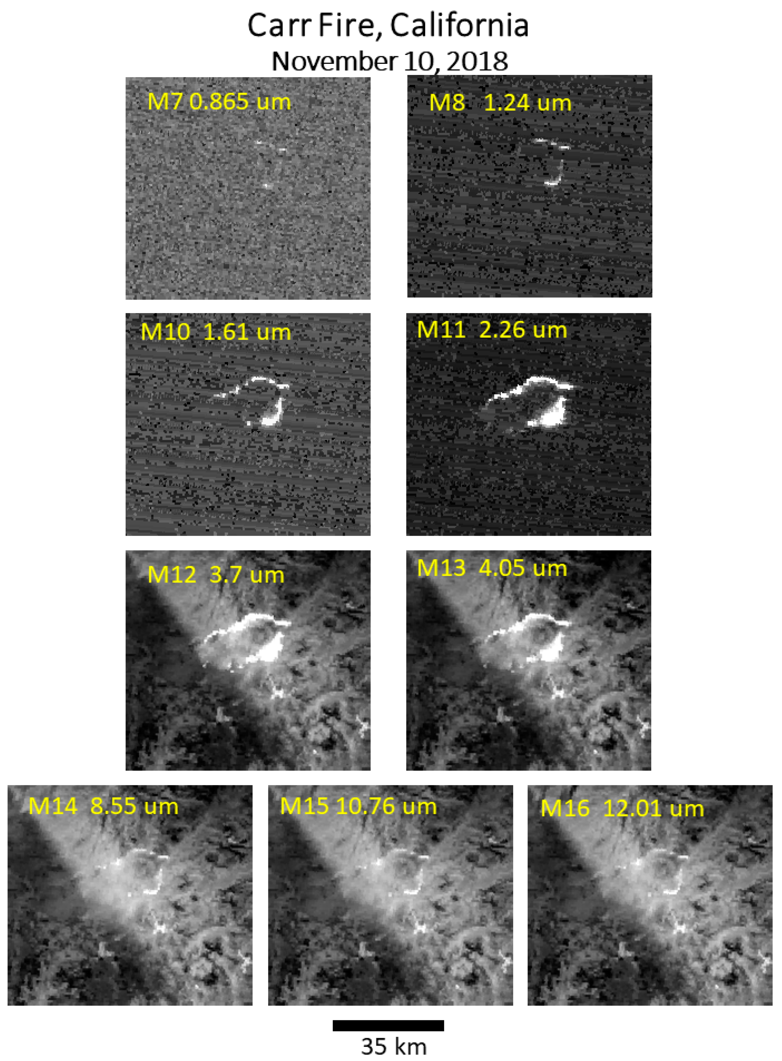
Carr FireCalifornia10-November-201839.7125 n121.4875 wSVM10_npp_d20181110_t0929507_e0935311_b36462
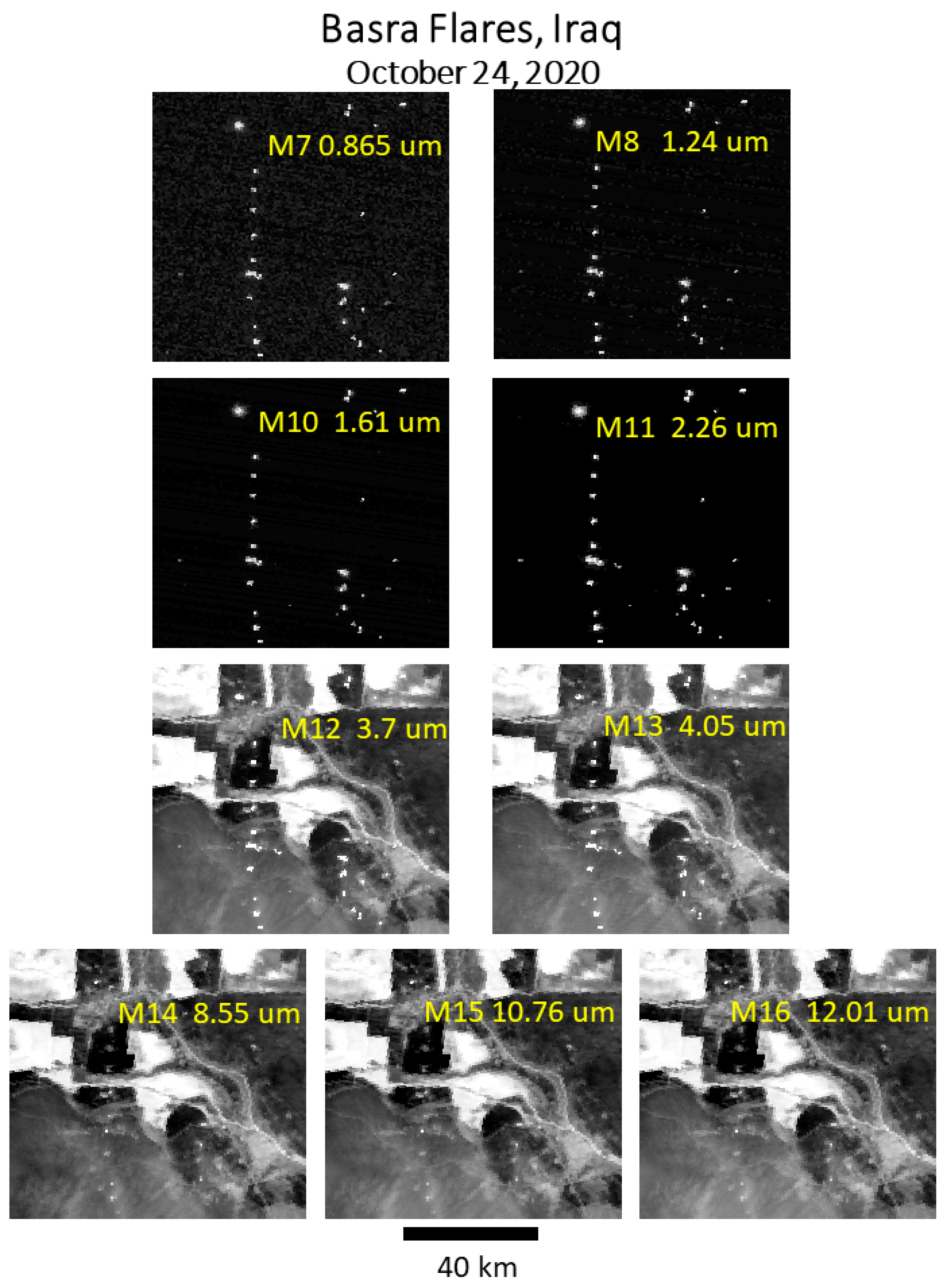
Basra FlaresIraq24-October-202030.6083 n47.325 eSVM10_j01_d20201024_t2225215_e2226442_b15203
Table 3. Scoring of the five methods.
Flaming SubtractiveTallyTriple Curve UnconstrainedTallyTriple Curve w/ Flaming K ConstraintTallyTriple Curve w/ Flaming K and Local Background K ConstraintsTallyTriple Curve w/ Local Background K ConstraintTally
Negative secondary esf66Primary .ge. 3000 K45Secondary less than 1 m283Secondary less than 350 K104Negative secondary esf65
Background under 260 K49Secondary less than 350 K108Secondary less than 350 K61Secondary less than 1 m294Secondary less than 350 K117
Secondary less than 350 K18Secondary less than 1 m2105Background less than 2608
Misfits133Misfits258Misfits152Misfits198Misfits182
% Yield67%% Yield37%% Yield63%% Yield51%% Yield55%
Publisher’s Note: MDPI stays neutral with regard to jurisdictional claims in published maps and institutional affiliations.

