Evaluating the Ability of FARSITE to Simulate Wildfires Influenced by Extreme, Downslope Winds in Santa Barbara, California

 , ,
, ,  ,
, 
 and
and
Abstract
:1. Introduction
2. Materials and Methods
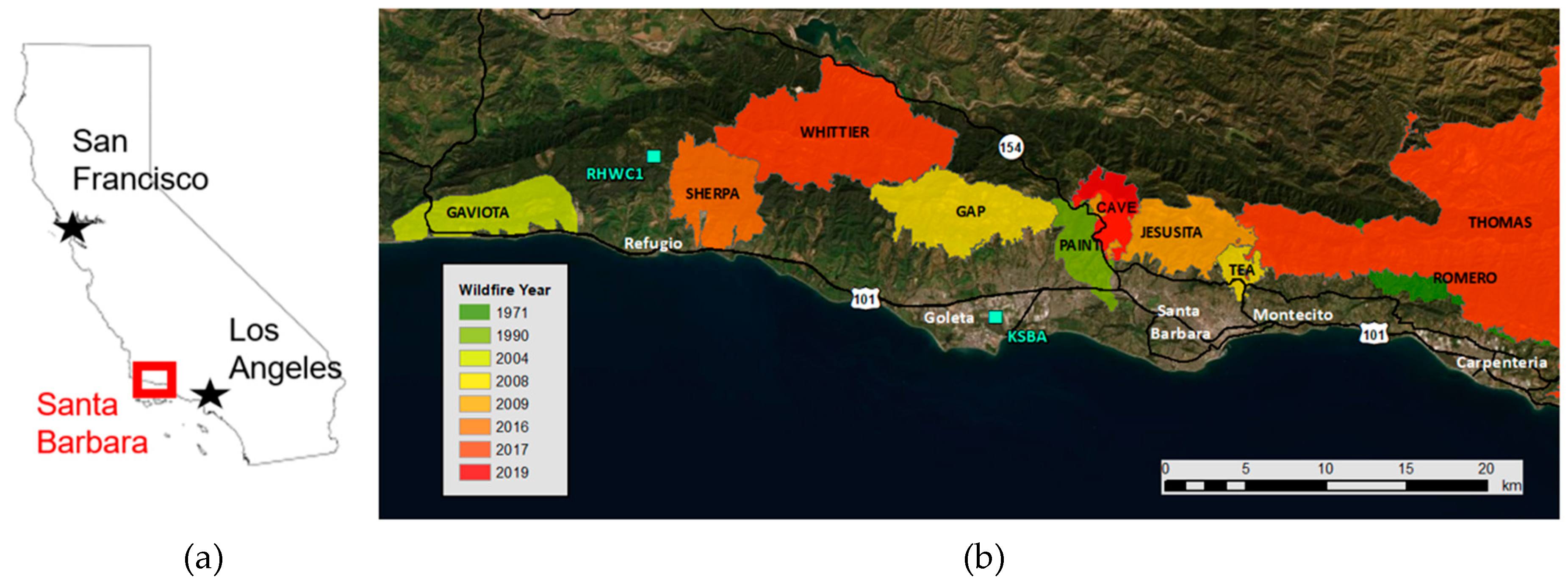
2.1. Case Studies
2.2. Wildland Fire Models
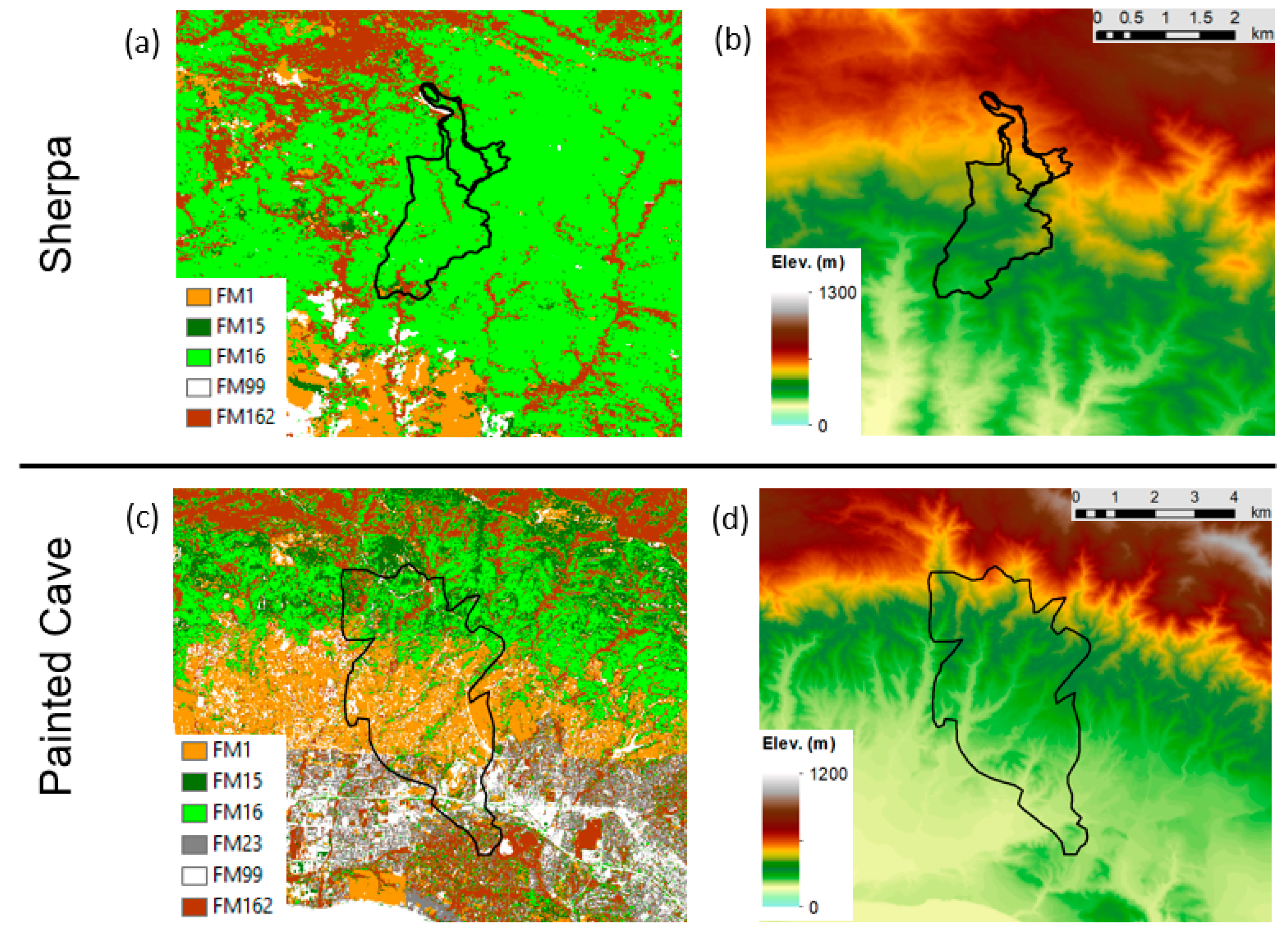
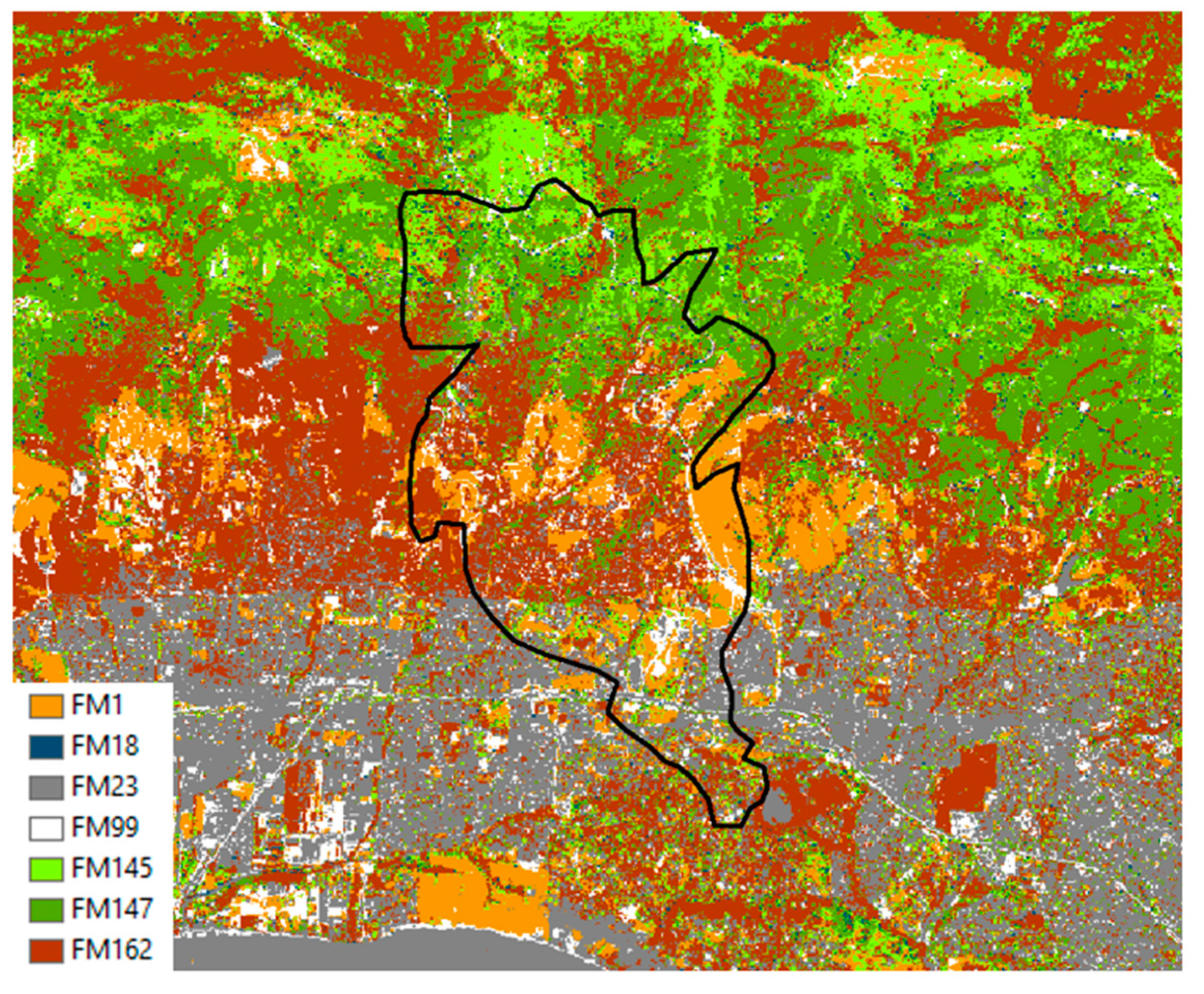
2.3. Fuel and Topography Data
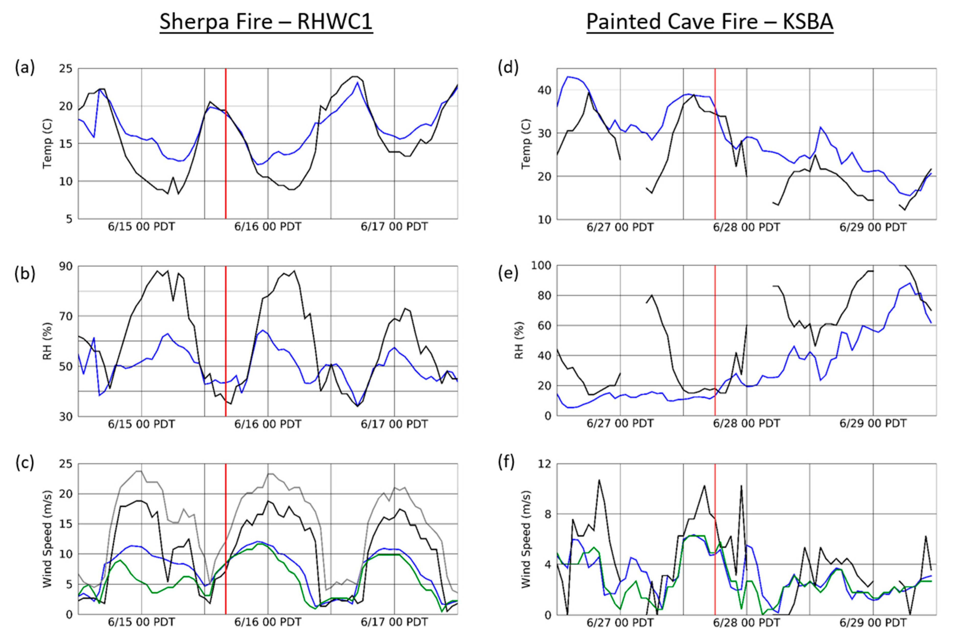
2.4. Weather Data
2.5. Gust Factor
2.6. Perimeter Data
3. Results and Discussion
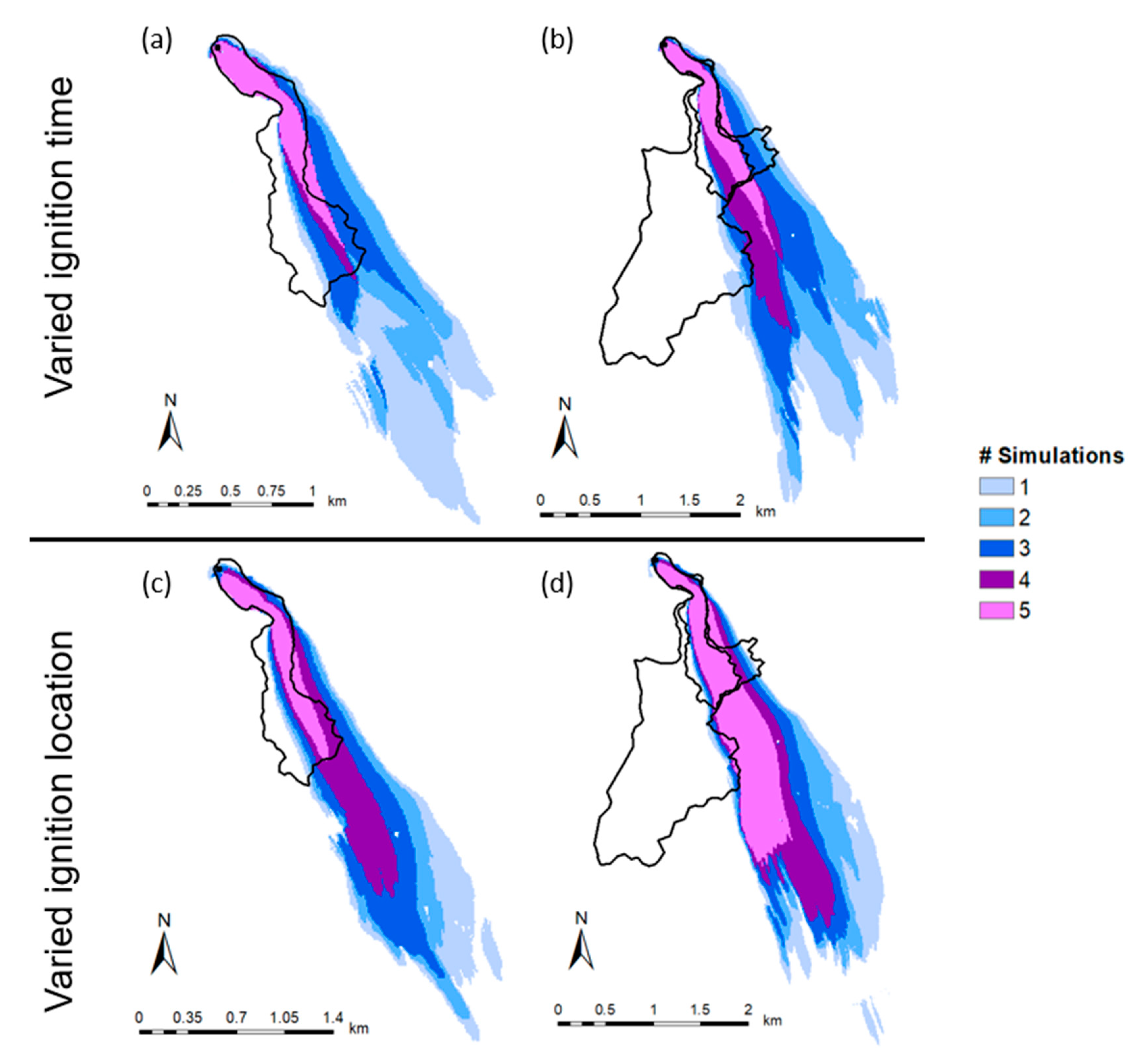
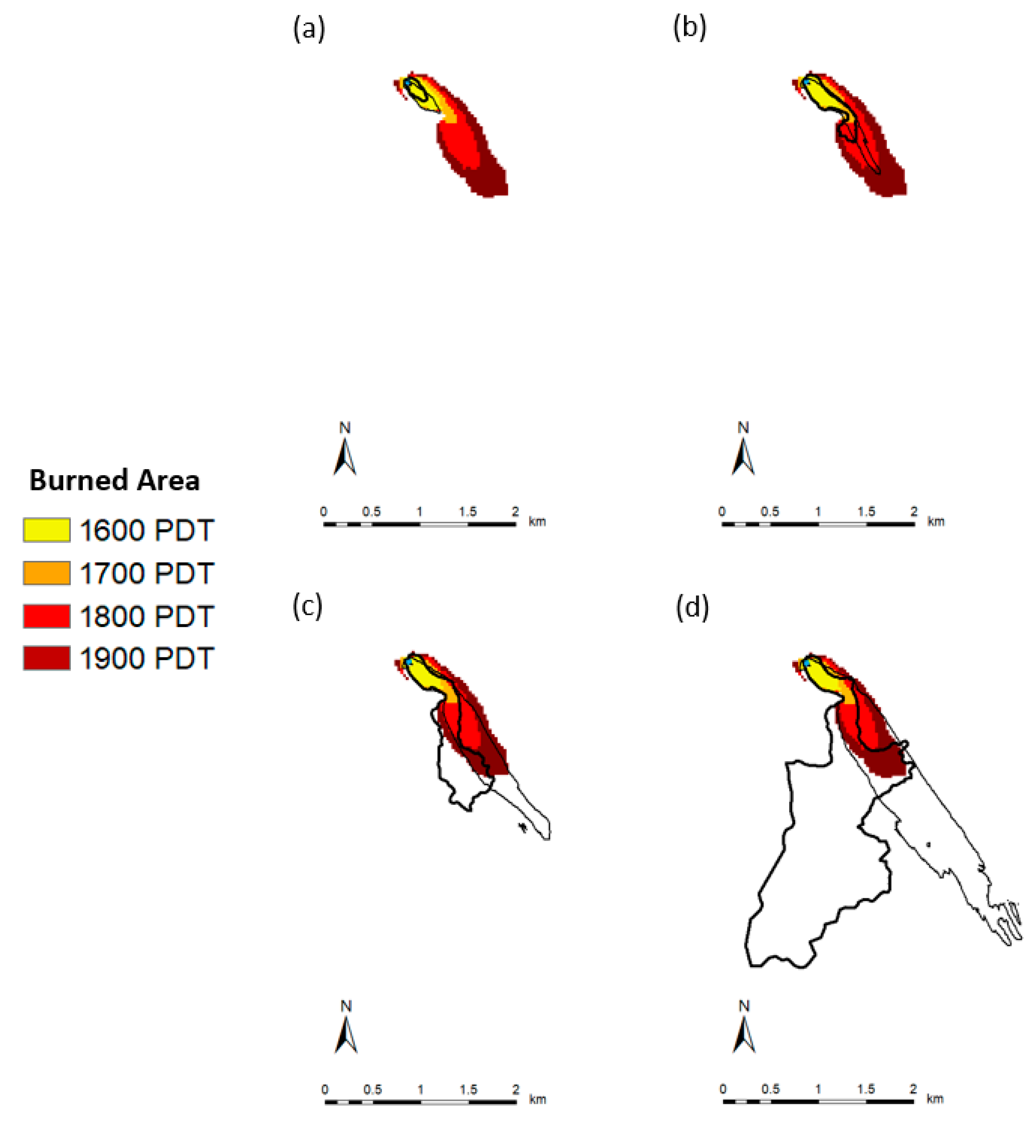
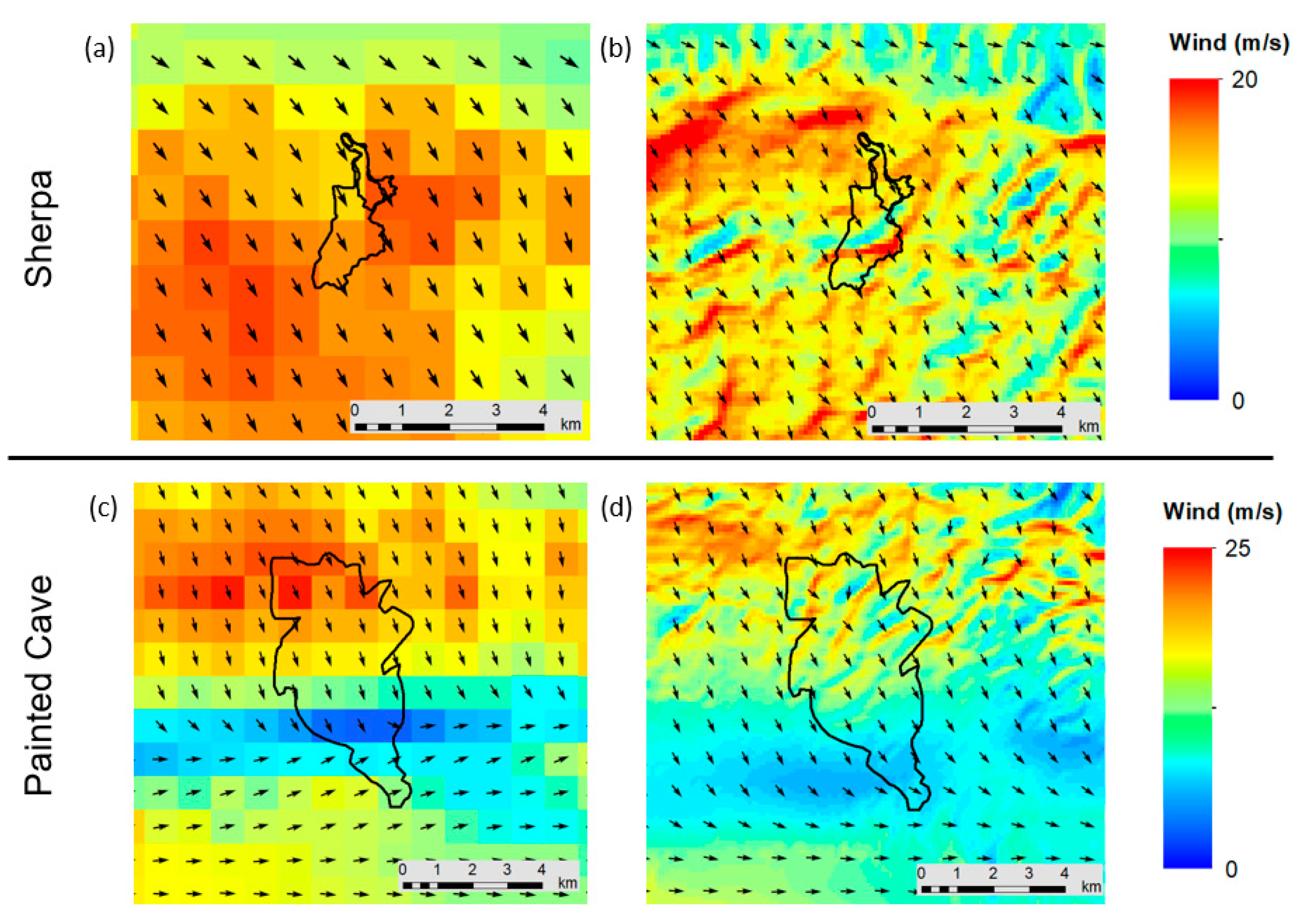
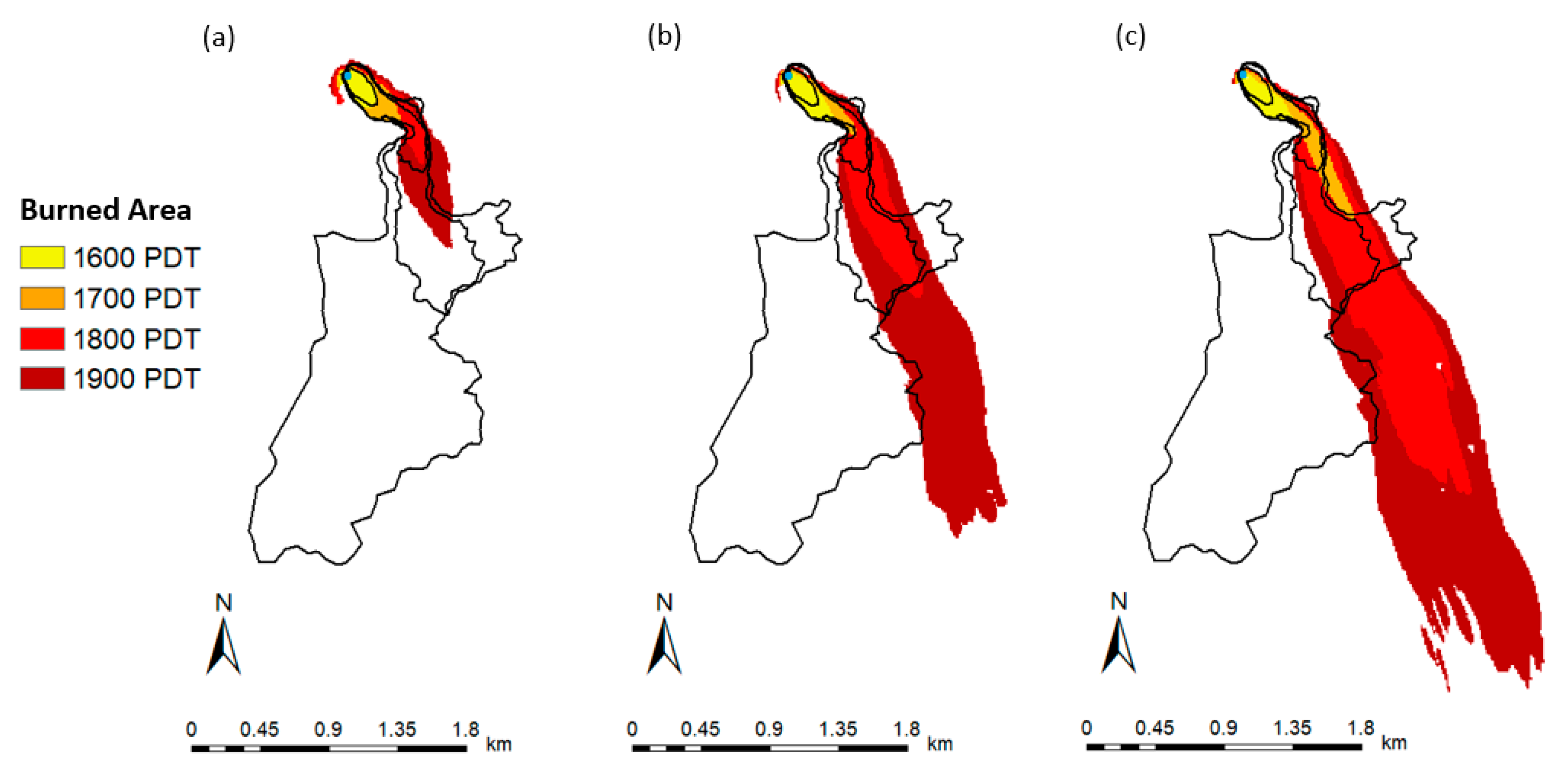
3.1. Sherpa Fire
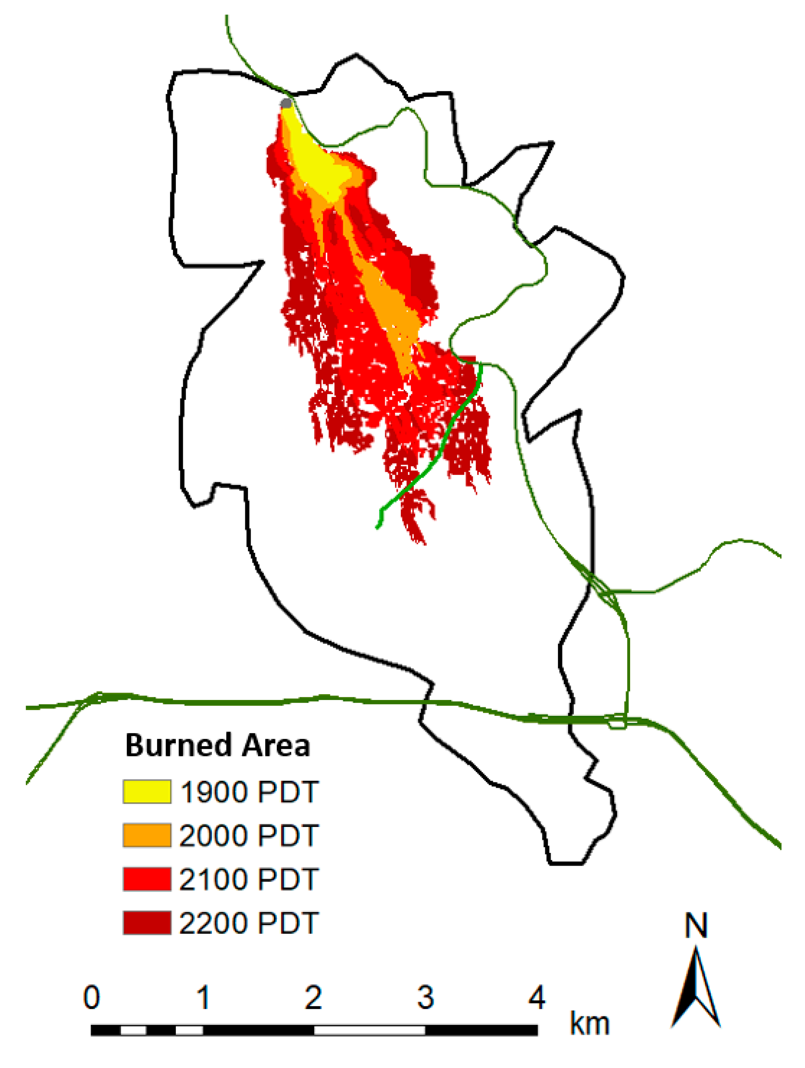
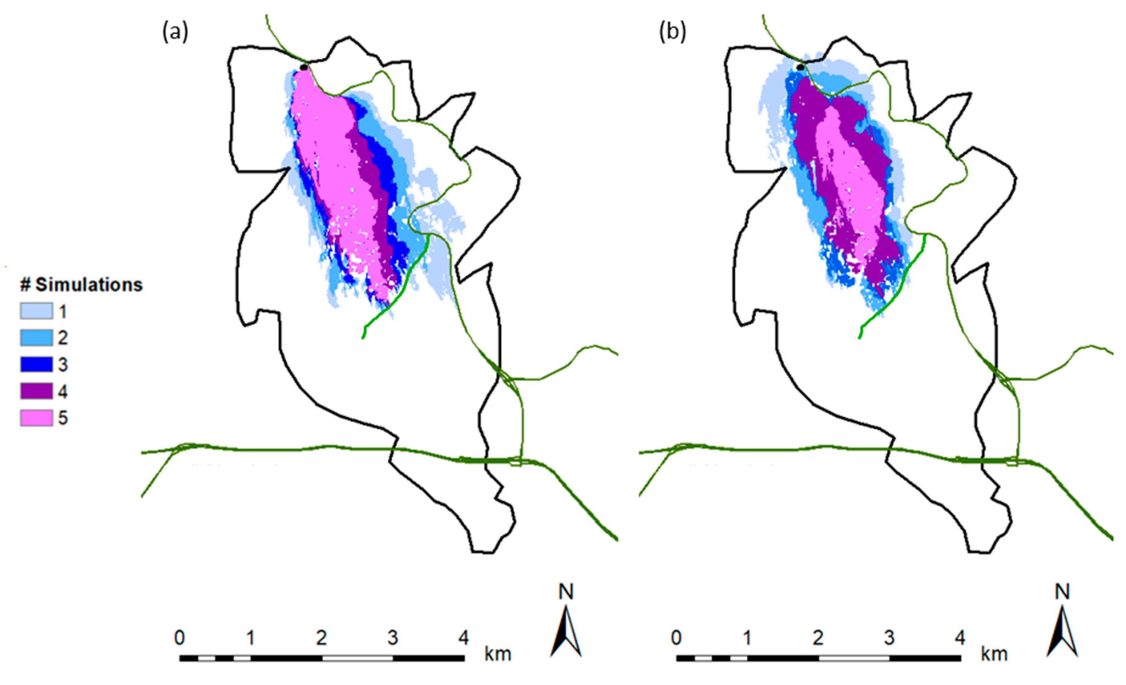
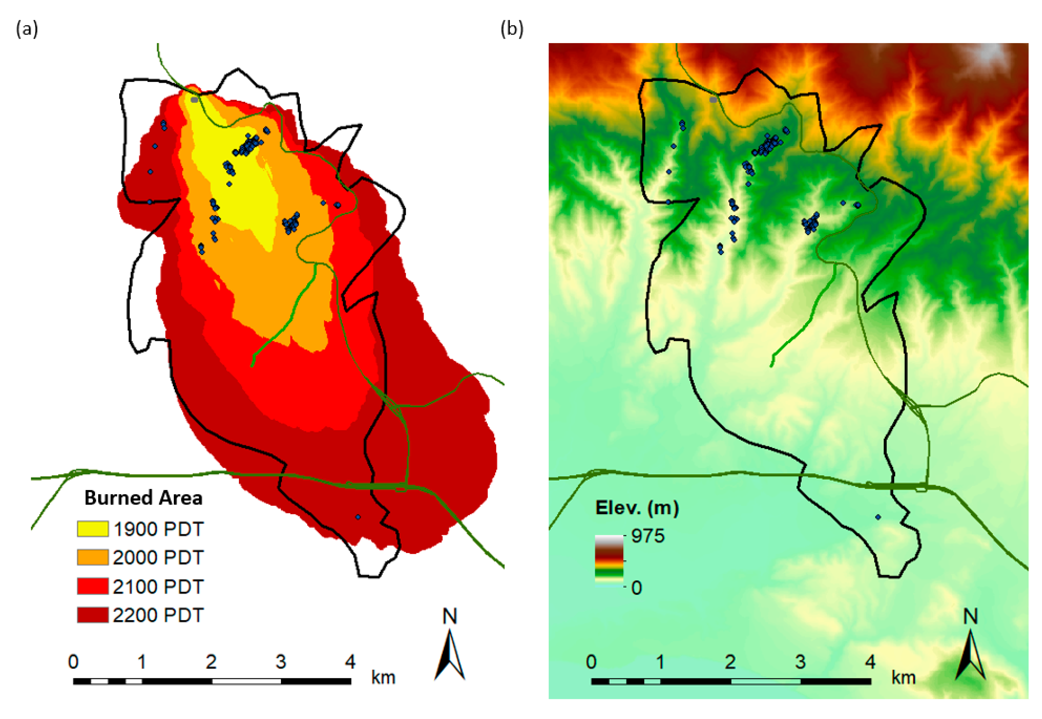
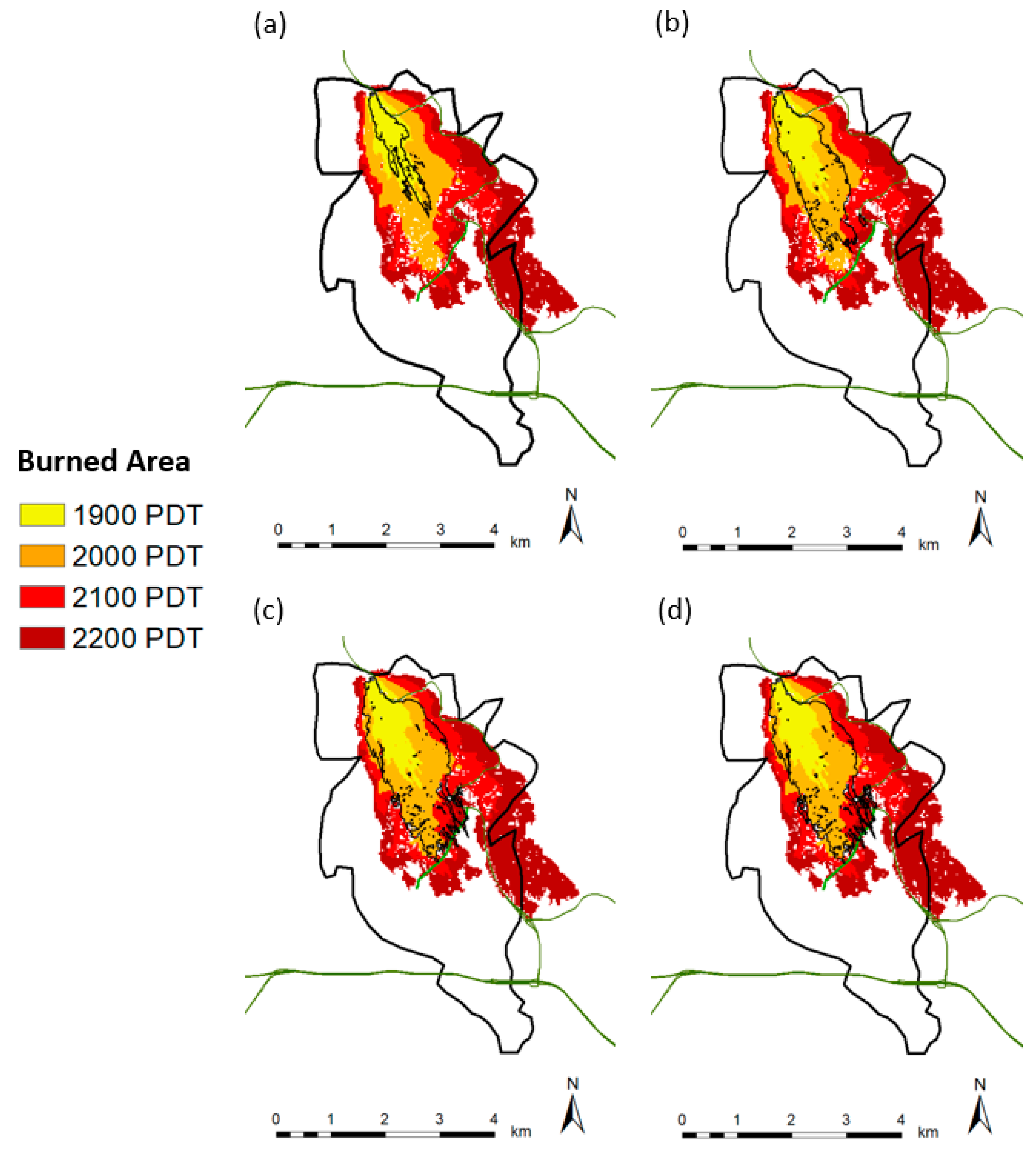
3.2. Painted Cave Fire
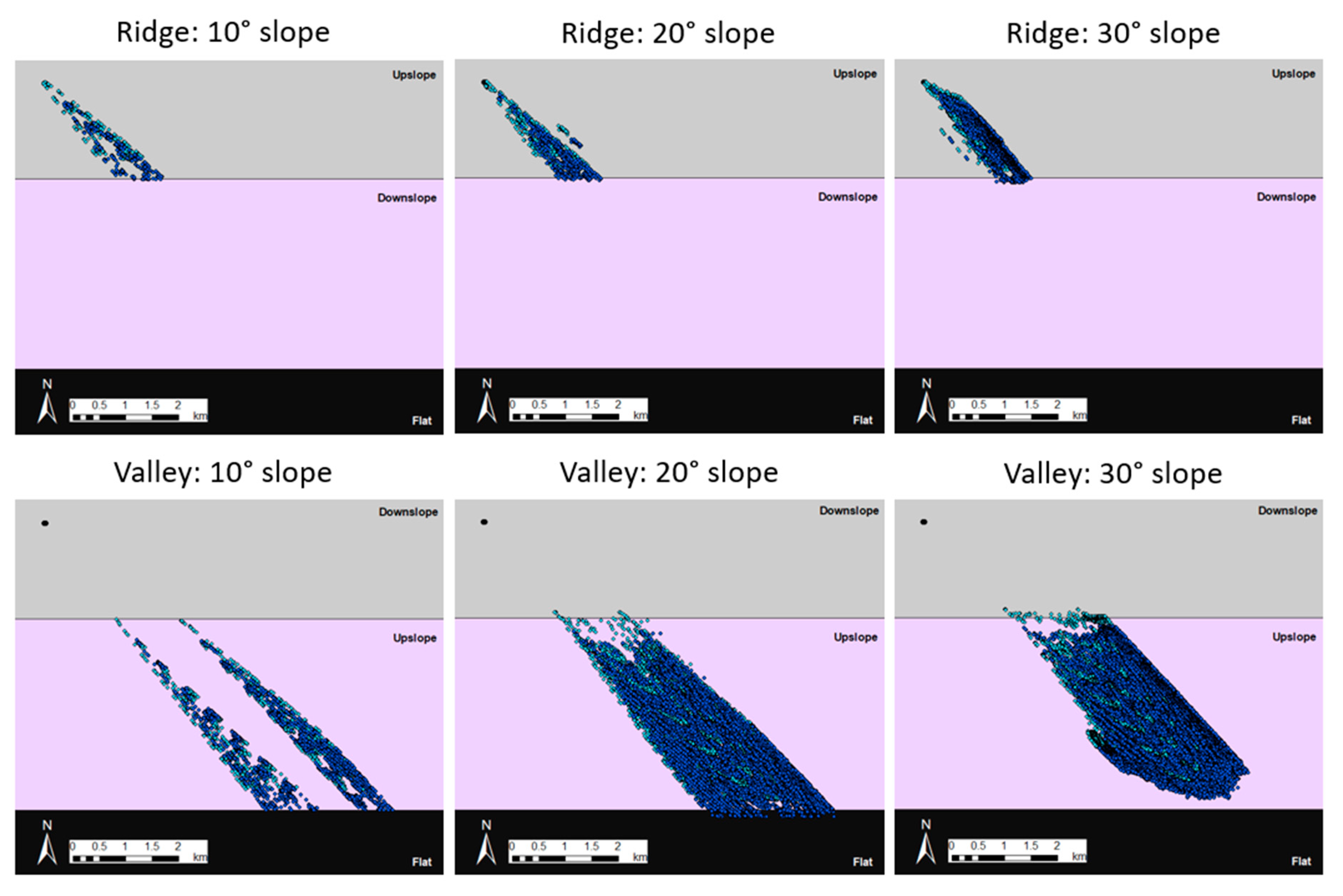
3.3. Spotting Limitations
3.4. FlamMap Comparisons
4. Conclusions
Author Contributions
Funding
Acknowledgments
Conflicts of Interest
Appendix

| ABBREVIATION | DESCRIPTION |
|---|---|
| FARSITE | Fire Area Simulator |
| FM | Fuel model |
| GF | Gust factor |
| KSBA | Santa Barbara Airport weather station |
| MTT | Minimum Travel Time |
| RAWS | Remote Automatic Weather Station |
| RHWC1 | Refugio weather station |
| SM | Sorensen Metric |
| SYM | Santa Ynez Mountains |
| WN | WindNinja |
| WRF | Weather Research and Forecasting model |


References
- Richardson, L.A.; Champ, P.A.; Loomis, J.B. The Hidden Cost of Wildfires: Economic Valuation of Health Effects of Wildfire Smoke Exposure in Southern California. JFE 2012, 18, 14–35. [Google Scholar] [CrossRef]
- Parise, M.; Cannon, S.H. Wildfire Impacts on the Processes That Generate Debris Flows in Burned Watersheds. Nat. Hazards 2012, 61, 217–227. [Google Scholar] [CrossRef]
- Westerling, A.L.; Hidalgo, H.G.; Cayan, D.R.; Swetnam, T.W. Warming and Earlier Spring Increase Western U.S. Forest Wildfire Activity. Science 2006, 313, 940–943. [Google Scholar] [CrossRef] [PubMed] [Green Version]
- Diffenbaugh, N.S.; Swain, D.L.; Touma, D. Anthropogenic Warming Has Increased Drought Risk in California. Proc. Natl. Acad. Sci. USA 2015, 112, 3931–3936. [Google Scholar] [CrossRef] [Green Version]
- Abatzoglou, J.T.; Williams, A.P. Impact of Anthropogenic Climate Change on Wildfire across Western US Forests. Proc. Natl. Acad. Sci. USA 2016, 113, 11770–11775. [Google Scholar] [CrossRef] [Green Version]
- Cayan, D.R.; Maurer, E.P.; Dettinger, M.D.; Tyree, M.; Hayhoe, K. Climate Change Scenarios for the California Region. Clim. Chang. 2008, 87 (Suppl. 1), 21–42. [Google Scholar] [CrossRef]
- Syphard, A.D.; Clarke, K.C.; Franklin, J. Simulating Fire Frequency and Urban Growth in Southern California Coastal Shrublands, USA. Landsc. Ecol. 2007, 22, 431–445. [Google Scholar] [CrossRef]
- Syphard, A.D.; Radeloff, V.C.; Keuler, N.S.; Taylor, R.S.; Hawbaker, T.J.; Stewart, S.I.; Clayton, M.K. Predicting Spatial Patterns of Fire on a Southern California Landscape. Int. J. Wildland Fire 2008, 17, 602. [Google Scholar] [CrossRef]
- Faivre, N.; Jin, Y.; Goulden, M.L.; Randerson, J.T. Controls on the Spatial Pattern of Wildfire Ignitions in Southern California. Int. J. Wildland Fire 2014, 23, 799. [Google Scholar] [CrossRef] [Green Version]
- Syphard, A.D.; Keeley, J.E. Location, Timing and Extent of Wildfire Vary by Cause of Ignition. Int. J. Wildland Fire 2015, 24, 37. [Google Scholar] [CrossRef]
- Countryman, C.M. The Fire Environment Concept; USDA Forest Service: Berkeley, CA, USA, 1972; p. 15. [Google Scholar]
- Rothermel, R.C. A Mathematical Model. for Predicting Fire Spread in Wildland Fuels; Research Paper INT-115; U.S. Department of Agriculture, Forest Service, Intermountain Forest and Range Experiment Station: Ogden, UT, USA, 1972; p. 40. [Google Scholar]
- Rothermel, R.C. How to Predict the Spread and Intensity of Forest and Range Fires; Research Paper INT-GTR-143; U.S. Department of Agriculture, Forest Service, Intermountain Forest and Range Experiment Station: Ogden, UT, USA, 1983. [Google Scholar]
- Catchpole, W.; Bradstock, R.; Choate, J.; Fogarty, L.; Gellie, N.; McCarthy, G.; McCaw, W.; Marsden-Smedley, J.; Pearce, G. Co-operative Development of Equations for Heathland Fire Behaviour. In Proceedings of the 3rd International Conference of Forest Fire Research, Luso, Portugal, 16–20 November 1998. [Google Scholar]
- Moritz, M.A. Spatiotemporal Analysis of Controls on Shrubland Fire Regimes: Age Dependency and Fire Hazard. Ecology 2003, 84, 351–361. [Google Scholar] [CrossRef]
- Keeley, J.E.; Safford, H.; Fotheringham, C.J.; Franklin, J.; Moritz, M. The 2007 southern California wildfires: Lessons in complexity. J. For. 2009, 107, 287–296. [Google Scholar]
- Stratton, R.D. Guidebook on LANDFIRE Fuels Data Acquisition, Critique, Modification, Maintenance, and Model. Calibration; Technical Report Np. RMRS-GTR-220; U.S. Department of Agriculture, Forest Service, Rocky Mountain Research Station: Fort Collins, CO, USA, 2009; pp. 1–54. [Google Scholar]
- Moritz, M.A.; Moody, T.J.; Krawchuk, M.A.; Hughes, M.; Hall, A. Spatial Variation in Extreme Winds Predicts Large Wildfire Locations in Chaparral Ecosystems: Extreme Winds and Large Wildfires. Geophys. Res. Lett. 2010, 37. [Google Scholar] [CrossRef] [Green Version]
- Ryan, G. Downslope Winds of Santa Barbara, California; NOAA Technical Memorandum NWS WR-240; Scientific Services Division, Western Region: Salt Lake City, UT, USA, 1996. [Google Scholar]
- Blier, W. The Sundowner Winds of Santa Barbara, California. Weather Forecast. 1998, 13, 702–716. [Google Scholar] [CrossRef]
- Hatchett, B.J.; Smith, C.M.; Nauslar, N.J.; Kaplan, M.L. Brief Communication: Synoptic-Scale Differences between Sundowner and Santa Ana Wind Regimes in the Santa Ynez Mountains, California. Nat. Hazards Earth Syst. Sci. 2018, 18, 419–427. [Google Scholar] [CrossRef] [Green Version]
- Smith, C.M.; Hatchett, B.J.; Kaplan, M.L. Characteristics of Sundowner Winds near Santa Barbara, California, from a Dynamically Downscaled Climatology: Environment and Effects near the Surface. J. Appl. Meteor. Climatol. 2018, 57, 589–606. [Google Scholar] [CrossRef]
- Sukup, S. Extreme Northeasterly Wind Events in the Hills above Montecito, California; Western Region Technical Attachment NWS WR-1302; NWS Western Region: Salt Lake City, UT, USA, 2013; p. 21. [Google Scholar]
- Cannon, F.; Carvalho, L.M.V.; Jones, C.; Hall, T.; Gomberg, D.; Dumas, J.; Jackson, M. WRF Simulation of Downslope Wind Events in Coastal Santa Barbara County. Atmos. Res. 2017, 191, 57–73. [Google Scholar] [CrossRef] [Green Version]
- Murray, A.T.; Carvalho, L.; Church, R.L.; Jones, C.; Roberts, D.A.; Xu, J.; Zigner, K.; Nash, D. Coastal vulnerability under extreme weather. In Applied Spatial analysis and Policy Special Issue: Contemporary Applications for Spatially Integrated Social Science; Springer: New York, NY, USA, (under review).
- Peterson, S.H. Fire Risk in California. Ph.D. Thesis, University of California, Santa Barbara, CA, USA, 2011. [Google Scholar]
- Finney, M.A. FARSITE: Fire Area Simulator-Model Development and Evaluation; Research Paper RMRS-RP-4; U.S. Department of Agriculture, Forest Service, Rocky Mountain Research Station: Fort Collins, CO, USA, 1998. [Google Scholar]
- Finney, M.A.; Bradshaw, L.; Butler, B.W. Modeling Surface Winds in Complex. Terrain for Wildland Fire Incident Support; Final Report for JFSP Funded Project #03-2-1-04; U.S. Department of Agriculture, Forest Service: Fort Collins, CO, USA, 2006; pp. 1–10. [Google Scholar]
- Stratton, R.D. Guidance on Spatial Wildland Fire Analysis: Models, Tools, and Techniques; General Technical Report RMRS-GTR-183; U.S. Department of Agriculture, Forest Service, Rocky Mountain Research Station: Ft. Collins, CO, USA, 2006. [Google Scholar] [CrossRef] [Green Version]
- Finney, M.A.; Ryan, K.C. Use of the FARSITE Fire Growth Model for Fire Prediction in U.S. National Parks. In Proceedings of the International Emergency Management and Engineering Conference, San Diego, CA, USA, 9–12 May 1995; pp. 183–189. [Google Scholar]
- Arca, B.; Duce, P.; Laconi, M.; Pellizzaro, G.; Salis, M.; Spano, D. Evaluation of FARSITE Simulator in Mediterranean Maquis. Int. J. Wildland Fire 2007, 16, 563. [Google Scholar] [CrossRef]
- Papadopoulos, G.D.; Pavlidou, F.-N. A Comparative Review on Wildfire Simulators. IEEE Syst. J. 2011, 5, 233–243. [Google Scholar] [CrossRef]
- Phillips, D.R.; Waldrop, T.A.; Simon, D.M. Assessment of the FARSTE model for predicting fire behavior in the Southern Appalachian Mountains. General Technical Report SRS-92. In Proceedings of the 13th Biennial Southern Silvicultural Research Conference; U.S. Department of Agriculture, Forest Service: Asheville, NC, USA, 2006; pp. 521–525. [Google Scholar]
- Forghani, A.; Cechet, B.; Radke, J.; Finney, M.; Butler, B. Applying Fire Spread Simulation over Two Study Sites in California Lessons Learned and Future Plans. In Proceedings of the 2007 IEEE International Geoscience and Remote Sensing Symposium, Barcelona, Spain, 23–28 July 2007; pp. 3008–3013. [Google Scholar] [CrossRef]
- Scott, J.H. Comparison of Crown Fire Modeling Systems Used in Three Fire Management Applications; RMRS-RP-58; U.S. Department of Agriculture, Forest Service, Rocky Mountain Research Station: Ft. Collins, CO, USA, 2006. [Google Scholar] [CrossRef] [Green Version]
- Coen, J.L.; Cameron, M.; Michalakes, J.; Patton, E.G.; Riggan, P.J.; Yedinak, K.M. WRF-Fire: Coupled Weather–Wildland Fire Modeling with the Weather Research and Forecasting Model. J. Appl. Meteor. Climatol. 2013, 52, 16–38. [Google Scholar] [CrossRef]
- Skamarock, W.C.; Klemp, J.B. A Time-Split Nonhydrostatic Atmospheric Model for Weather Research and Forecasting Applications. J. Comput. Phys. 2008, 227, 3465–3485. [Google Scholar] [CrossRef]
- Kochanski, A.K.; Jenkins, M.A.; Mandel, J.; Beezley, J.D.; Krueger, S.K. Real Time Simulation of 2007 Santa Ana Fires. For. Ecol. Manag. 2013, 294, 136–149. [Google Scholar] [CrossRef] [Green Version]
- Gollner, M.; Trouv’e, A.; Altintas, I.; Block, J.; De Callafon, R.; Clements, C.; Cortes, A.; Ellicott, E.; Filippi, J.B.; Finney, M.; et al. Towards data-driven operational wildfire spread modeling. In Report of the NSF-Funded Wildfire Workshop; University of Maryland: College Park, MD, USA, 2015. [Google Scholar]
- Hazard, R.; Chief of Santa Barbara County Fire Department, Santa Barbara, CA, USA. Personal communication, 2019.
- Anderson, H.E. Aids to Determining Fuel Models for Estimating Fire Behavior; General Technical Report INT-GTR-122; U.S. Department of Agriculture, Forest Service, Intermountain Forest and Range Experiment Station: Ogden, UT, USA, 1982. [Google Scholar] [CrossRef] [Green Version]
- Van Wagner, C.E. Conditions for the start and spread of crown fire. Can. J. For. Res. 1977, 7, 23–34. [Google Scholar] [CrossRef]
- Albini, F.A. Spot Fire Distance from Burning Trees: A Predictive Model; Intermountain Forest and Range Experiment Station, Forest Service, U.S. Department of Agriculture: Ogden, UT, USA, 1979; Volume 56. [Google Scholar]
- Andrews, P.L. BehavePlus Fire Modeling System: Past, Present, and Future. In Proceedings of the 7th Symposium on Fire and Forest Meteorological Society, Bar Harbor, ME, USA, 23–25 October 2007. [Google Scholar]
- Hanes, T.L. Ecological Studies on Two Closely Related Chaparral Shrubs in Southern California. Ecol. Monogr. 1965, 35, 213–235. [Google Scholar] [CrossRef]
- Hanes, T.L. The Vegetation Called Chaparral. In Proceedings of the Symposium on Living with the Chaparral, Sierra Club, San Francisco, CA, USA, 30–31 March 1973; pp. 1–5. [Google Scholar]
- Rothermel, R.C.; Philpot, C.W. Predicting Changes in Chaparral Flammability. J. For. 1973, 71, 640–643. [Google Scholar]
- Countryman, C.M.; Philpot, C.W. Physical Characteristics of Chamise as a Wildland Fuel; Res. Pap. PSW-66; U.S. Department of Agriculture Forest Service: Berkeley, CA, USA, 1970. [Google Scholar]
- Meerdink, S.K.; Roberts, D.A.; Roth, K.L.; King, J.Y.; Gader, P.D.; Koltunov, A. Classifying California plant species temporally using airborne hyperspectral imagery. Remote Sens. Environ. 2019, 232, 111308. [Google Scholar] [CrossRef]
- Roth, K.L.; Dennison, P.E.; Roberts, D.A. Comparing Endmember Selection Techniques for Accurate Mapping of Plant Species and Land Cover Using Imaging Spectrometer Data. Remote Sens. Environ. 2012, 127, 139–152. [Google Scholar] [CrossRef]
- Peterson, S.H.; Stow, D.A. Using Multiple Image Endmember Spectral Mixture Analysis to Study Chaparral Regrowth in Southern California. Int. J. Remote Sens. 2003, 24, 4481–4504. [Google Scholar] [CrossRef]
- Scott, J.H.; Burgan, R.E. Standard Fire Behavior Fuel Models: A Comprehensive Set for Use with Rothermel’s Surface Fire Spread Model; General Technical Report RMRS-GTR-153; U.S. Department of Agriculture, Forest Service, Rocky Mountain Research Station: Ft. Collins, CO, USA, 2005. [Google Scholar] [CrossRef]
- Weise, D.R.; Regelbrugge, J. Recent Chaparral Fuel Modeling Efforts. In Chaparral Fuel Modeling Workshop; 1997; pp. 11–12. Available online: http://web.physics.ucsb.edu/~complex/research/hfire/fuels/refs/weiseregel1997.pdf (accessed on 9 July 2020).
- Farr, T.G.; Rosen, P.A.; Caro, E.; Crippen, R.; Duren, R.; Hensley, S.; Kobrick, M.; Paller, M.; Rodriguez, E.; Roth, L.; et al. The Shuttle Radar Topography Mission. Rev. Geophys. 2007, 45. [Google Scholar] [CrossRef] [Green Version]
- Duine, G.J.; Jones, C.; Carvalho, L.; Fovell, R. Simulating Sundowner Winds in Coastal Santa Barbara: Model Validation and Sensitivity. Atmosphere 2019, 10, 155. [Google Scholar] [CrossRef] [Green Version]
- Gibson, C.; Gorski, C. FARSITE Weather Streams from the NWS IFPS System. In Proceedings of the 5th Symposium on Fire and Forest Meteorology; 2003; pp. 1–4. Available online: https://gacc.nifc.gov/nwcc/content/products/intelligence/FARSITE_Wx_DataGenerator.pdf (accessed on 9 July 2020).
- Carvalho, L.; Duine, G.-J.; Jones, C.; Zigner, K.; Clements, C.; Kane, H.; Gore, C.; Bell, G.; Gamelin, B.; Gomberg, D.; et al. The Sundowner Winds Experiment (SWEX) Pilot Study: Understanding Downslope Windstorms in the Santa Ynez Mountains, Santa Barbara, California. Mon. Wea. Rev. 2020, 148, 1519–1539. [Google Scholar] [CrossRef]
- Butler, B.W.; Forthofer, J.M. Gridded Wind Data: What Is It and How Is It Used? Report on file; U.S. Department of Agriculture, Forest Service, Rocky Mountain Research Station, Fire Sciences Lab.: Missoula, MT, USA, 2004. [Google Scholar]
- Salis, M. Fire Behavior Simulation in Mediterranean Marquis using FARSITE. Ph.D. Thesis, University of Sassari, Sassari, Italy, 2008. [Google Scholar]
- Forthofer, J.M.; Butler, B.W.; Wagenbrenner, N.S. A Comparison of Three Approaches for Simulating Fine-Scale Surface Winds in Support of Wildland Fire Management. Part I. Model Formulation and Comparison against Measurements. Int. J. Wildland Fire 2014, 23, 969. [Google Scholar] [CrossRef]
- Forthofer, J.M.; Shannon, K.; Butler, B.W. Simulating Diurnally Driven Slope Winds with WindNinja; U.S. Department of Agriculture, Forest Service, Rocky Mountain Research Station: Missoula, MT, USA, 2009. [Google Scholar]
- Butler, B.W.; Forthofer, J.M.; Finney, M.; McHugh, C.; Stratton, R.; Bradshaw, L. The impact of high resolution wind field simulations on the accuracy of fire growth predictions. For. Ecol. Manag. 2006, 234, S85. [Google Scholar] [CrossRef]
- Jahdi, R.; Darvishsefat, A.A.; Etemad, V.; Mostafavi, M.A. Wind Effect on Wildfire and Simulation of Its Spread (Case Study: Siahkal Forest in Northern Iran). J. Agric. Sci. Technol. 2014, 16, 1109–1121. [Google Scholar]
- Forthofer, J.M.; Butler, B.W.; McHugh, C.W.; Finney, M.A.; Bradshaw, L.S.; Stratton, R.D.; Shannon, K.S.; Wagenbrenner, N.S. A Comparison of Three Approaches for Simulating Fine-Scale Surface Winds in Support of Wildland Fire Management. Part II. An Exploratory Study of the Effect of Simulated Winds on Fire Growth Simulations. Int. J. Wildland Fire 2014, 23, 982. [Google Scholar] [CrossRef]
- Horel, J.; Splitt, M.; Dunn, L.; Pechmann, J.; White, B.; Ciliberti, C.; Lazarus, S.; Slemmer, J.; Zaff, D.; Burks, J. Mesowest: Cooperative Mesonets in the Western United States. Bull. Am. Meteorol. Soc. 2002, 83, 211–226. [Google Scholar] [CrossRef]
- Westerling, A.L.; Cayan, D.R.; Brown, T.J.; Hall, B.L.; Riddle, L.G. Climate, Santa Ana Winds and Autumn Wildfires in Southern California. Eostransactions Am. Geophys. Union 2004, 85, 289–296. [Google Scholar] [CrossRef]
- Mitchell, J.W. Power Line Failures and Catastrophic Wildfires under Extreme Weather Conditions. Eng. Fail. Anal. 2013, 35, 726–735. [Google Scholar] [CrossRef]
- Fovell, R.G.; Cao, Y. The Santa Ana Winds of Southern California: Winds, Gusts, and the 2007 Witch Fire. Wind Struct. 2017, 24, 529–564. [Google Scholar] [CrossRef]
- Cao, Y.; Fovell, R.G. Downslope Windstorms of San Diego County. Part II: Physics Ensemble Analyses and Gust Forecasting. Weather Forecast. 2018, 33, 539–559. [Google Scholar] [CrossRef]
- Fovell, R.; Gallagher, A. Winds and Gusts during the Thomas Fire. Fire 2018, 1, 47. [Google Scholar] [CrossRef] [Green Version]
- Santa Barbara County Fire Department. Available online: https://www.sbcfire.com (accessed on 10 June 2020).
- Greig-Smith, P. Quantitative Plant. Ecology; University of California Press: Berkeley, CA, USA, 1983; Volume 9. [Google Scholar]
- Perry, G.L.W.; Sparrow, A.D.; Owens, I.F. A GIS-Supported Model for the Simulation of the Spatial Structure of Wildland Fire, Cass Basin, New Zealand. J. Appl. Ecol. 1999, 36, 502–518. [Google Scholar] [CrossRef]
- Peterson, S.H.; Morais, M.E.; Carlson, J.M.; Dennison, P.E.; Roberts, D.A.; Moritz, M.A.; Weise, D.R. Using HFire for Spatial Modeling of Fire in Shrublands; Research Paper PSW-RP-259; U.S. Department of Agriculture, Forest Service, Pacific Southwest Research Station: Albany, CA, USA, 2009. [Google Scholar] [CrossRef]
- Salis, M.; Ager, A.A.; Arca, B.; Finney, M.A.; Bacciu, V.; Duce, P.; Spano, D. Assessing Exposure of Human and Ecological Values to Wildfire in Sardinia, Italy. Int. J. Wildland Fire 2013, 22, 549. [Google Scholar] [CrossRef]
- Salis, M.; Arca, B.; Alcasena, F.; Arianoutsou, M.; Bacciu, V.; Duce, P.; Duguy, B.; Koutsias, N.; Mallinis, G.; Mitsopoulos, I.; et al. Predicting Wildfire Spread and Behaviour in Mediterranean Landscapes. Int. J. Wildland Fire 2016, 25, 1015–1032. [Google Scholar] [CrossRef]
- Stephens, S.L.; Weise, D.R.; Fry, D.L.; Keiffer, R.J.; Dawson, J.; Koo, E.; Potts, J.; Pagni, P.J. Measuring the Rate of Spread of Chaparral Prescribed Fires in Northern California. Fire Ecol. 2008, 4, 74–86. [Google Scholar] [CrossRef]
- Finney, M.A. Efforts at Comparing Simulated and Observed Fire Growth Patterns; Final Report INT-95066-RJVA; Systems for Environmental Management: Missoula, MT, USA, 1998. [Google Scholar]
- Fujioka, F.; Chapman University, Orange, CA, USA. Personal communication, 2020.


| Fire | Date | Acres Burned | Structural Impacts | Injuries and Deaths |
|---|---|---|---|---|
| Painted Cave | June 1990 | 2000 ha | 427 destroyed | 1 death |
| Tea | November 2008 | 785 ha | 210 destroyed | - |
| Jesusita | May 2009 | 3500 ha | 80 destroyed | - |
| Sherpa | June 2016 | 3200 ha | 1 destroyed | 1 injury |
| Thomas | December 2017 | 110,000 ha | 1000 destroyed | 2 deaths |
| Cave | November 2019 | 1265 ha | - | - |
| Vegetation Name | Fuel Model Number | Fuel Model Source | Fuel Model Name | Fuel Model Code |
|---|---|---|---|---|
| Short Grass | 1 | Anderson | - | - |
| Chamise | 15 | Weise and Regelbrugge | - | - |
| Ceanothus | 16 | Weise and Regelbrugge | - | - |
| Coastal Sage Scrub | 18 | Weise and Regelbrugge | - | - |
| Suburban/WUI | 23 | Scott and Burgan | Moderate Load Conifer Litter | TL3 |
| Shrubs | 145 | Scott and Burgan | High Load, Dry Climate Shrub | SH5 |
| Dense Shrubs | 147 | Scott and Burgan | Very High Load, Dry Climate Shrub | SH7 |
| Trees/Riparian | 162 | Scott and Burgan | Timber-Understory | TU2 |
| Distance Resolution | 30 m |
|---|---|
| Perimeter Resolution | 30 m |
| Time Step | 10 min |
| Fuel Properties | |
| Canopy Cover | 10% |
| Stand Height | 3 m |
| Base Stand Height | 0.1 m |
| Canopy Bulk Density | 0.2 kg m−3 |
| Foliar Moisture Content | 50% |
| Spotting Settings | |
| Spot Probability | 5 % |
| Spot Delay | 0 min |
| Min. Spot Distance | 12 m |
| Background Spot Grid Resolution | 6 m |
| Burned Area (ha) | SM | |||||||
| SHERPA | 1600 | 1700 | 1800 | 1900 | 1600 | 1700 | 1800 | 1900 |
| Observed Perimeters | 3.0 | 11.8 | 46.6 | 246.6 | - | - | - | - |
| 1.0 GF | 3.8 | 8.0 | 13.8 | 33.0 | 0.84 | 0.66 | 0.37 | 0.17 |
| 1.4 GF | 5.1 | 8.2 | 32.9 | 128.6 | 0.64 | 0.68 | 0.64 | 0.25 |
| 1.7 GF | 5.2 | 14.3 | 95.2 | 237.5 | 0.57 | 0.68 | 0.40 | 0.21 |
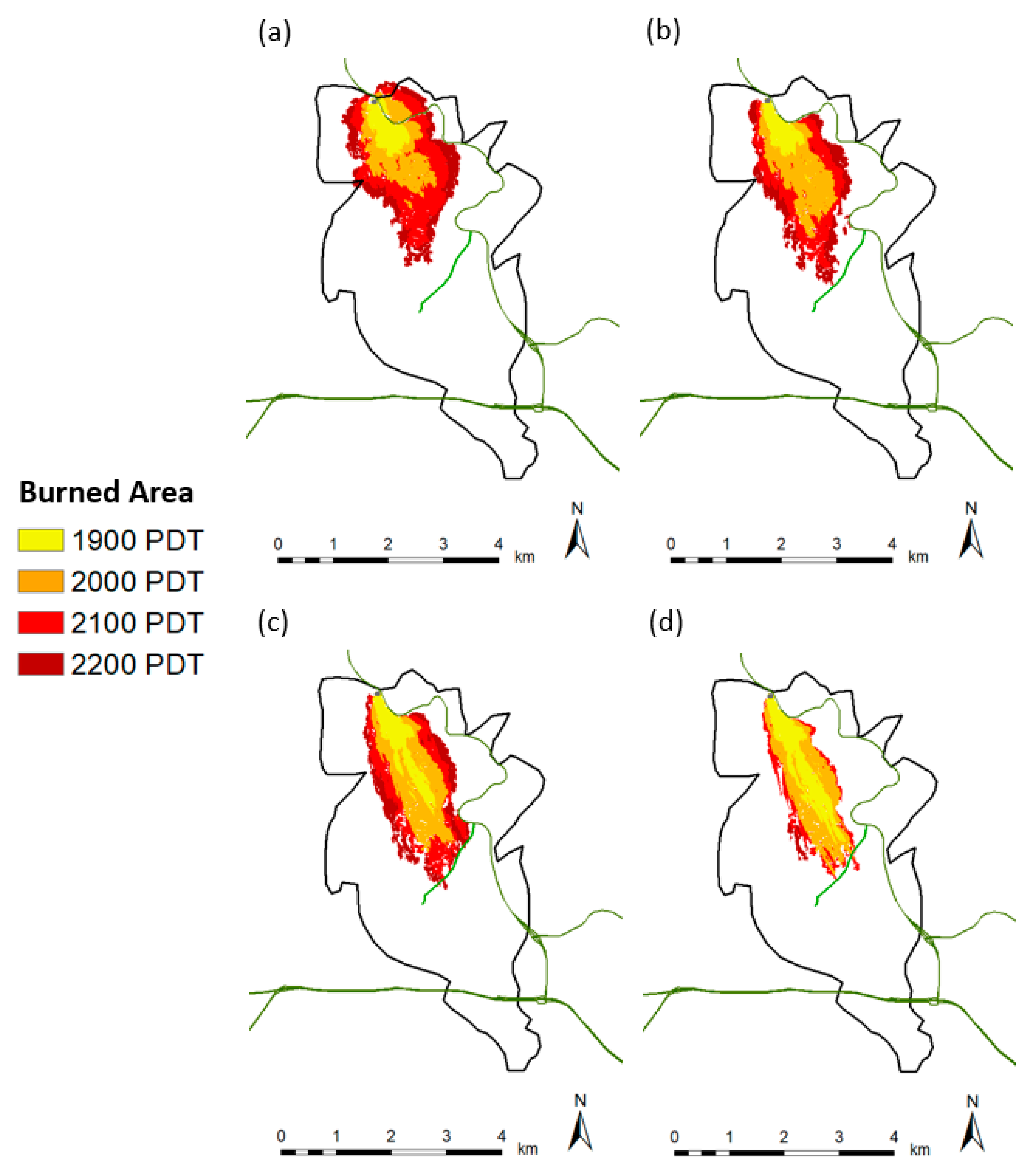
| Burned Area (ha) | SM | |||||||
| PAINTED CAVE | 1900 | 2000 | 2100 | 2200 | 1900 | 2000 | 2100 | 2200 |
| Observed Perimeter | 1792 (final) | 1792 (final) | 1792 (final) | 1792 (final) | - | - | - | - |
| 1.0 GF | 37 | 153 | 296 | 407 | 0.05 | 0.16 | 0.28 | 0.37 |
| 1.4 GF | 43 | 162 | 265 | 351 | 0.04 | 0.17 | 0.26 | 0.33 |
| 1.7 GF | 64 | 195 | 298 | 380 | 0.07 | 0.20 | 0.29 | 0.36 |
| 2.0 GF | 95 | 210 | 247 | 256 | 0.10 | 0.21 | 0.24 | 0.25 |
| 1.7 GF—all FM1 | 156 | 587 | 1097 | 1720 | 0.16 | 0.49 | 0.71 | 0.76 |
© 2020 by the authors. Licensee MDPI, Basel, Switzerland. This article is an open access article distributed under the terms and conditions of the Creative Commons Attribution (CC BY) license (http://creativecommons.org/licenses/by/4.0/).
Share and Cite
Zigner, K.; Carvalho, L.M.V.; Peterson, S.; Fujioka, F.; Duine, G.-J.; Jones, C.; Roberts, D.; Moritz, M. Evaluating the Ability of FARSITE to Simulate Wildfires Influenced by Extreme, Downslope Winds in Santa Barbara, California. Fire 2020, 3, 29. https://doi.org/10.3390/fire3030029
Zigner K, Carvalho LMV, Peterson S, Fujioka F, Duine G-J, Jones C, Roberts D, Moritz M. Evaluating the Ability of FARSITE to Simulate Wildfires Influenced by Extreme, Downslope Winds in Santa Barbara, California. Fire. 2020; 3(3):29. https://doi.org/10.3390/fire3030029
Chicago/Turabian StyleZigner, Katelyn, Leila M. V. Carvalho, Seth Peterson, Francis Fujioka, Gert-Jan Duine, Charles Jones, Dar Roberts, and Max Moritz. 2020. "Evaluating the Ability of FARSITE to Simulate Wildfires Influenced by Extreme, Downslope Winds in Santa Barbara, California" Fire 3, no. 3: 29. https://doi.org/10.3390/fire3030029
APA StyleZigner, K., Carvalho, L. M. V., Peterson, S., Fujioka, F., Duine, G.-J., Jones, C., Roberts, D., & Moritz, M. (2020). Evaluating the Ability of FARSITE to Simulate Wildfires Influenced by Extreme, Downslope Winds in Santa Barbara, California. Fire, 3(3), 29. https://doi.org/10.3390/fire3030029