1. Introduction
Wildfires continue to impact communities across the globe, requiring vast resources and extended suppression efforts. In response, both fire services and regulators have invested in research, policy, and operational responses designed to mitigate the significant impacts of these often fatal disasters. One approach adopted in areas identified as being prone to wildfire is the enhancement of residential construction standards in an effort to provide protective shelters for families within their own homes [
1,
2,
3].
These construction standards are based on the empirically calculated radiant heat and ember impact within 100 m of the approaching wildfire front. In order to determine the level of wildfire resistant construction required under the Building Code of Australia, [
2,
3] first provide empirical wildfire models for treed, heath, and grasslands fuel structures that subsequently calculate inputs for a single wildfire radiation model used to determine radiant heat flux. The level of radiant heat flux corresponds to various “Bushfire Attack Levels”, which subsequently prescribe the enhancements required to the normal construction standard [
1]. As the calculated radiant heat flux increases, so does the Bushfire Attack Level and resulting required construction standards. The construction standards identified in each of the Bushfire Attack Levels all assume ember impact, which are incorporated into the relevant dwelling designs. As opposed to relying on fire engineers to determine various design wildfires for analysis, [
2,
3] both require the assumption of the absolute worst case scenario, regardless of how realistic it may be.
The models such as those described in [
2,
3] assume fire growth is unrestricted by vegetation fuel bed geometry; the head fire has attained a quasi-steady rate of spread; and the shielding effects of urban development are ignored. Whilst this conservative approach is suitable for developments in regional areas surrounded by expansive state forest or plantation, its application without modification is not appropriate to small vegetation fires in urban areas, such as those in road reserves, urban parklands, verges, landscaped gardens, and other similar scenarios where vegetation fuel bed geometry restricts fire growth [
4]. Initial analysis of satellite imagery suggests the issues identified in [
4,
5] may potentially affect widespread urban areas within all major cities of Australia. This suggestion is supported by fire services incident reporting data, which identified that in Western Australia between 1998–2008, there were 24,784 vegetation fires within metropolitan urban and peri-urban areas, a total area of less than one hectare [
6], whereby multiple factors (not simply fire suppression alone) prevented unrestricted wildfire growth. In these scenarios, and without modification as reported in this paper, the models of [
2,
3] will be likely to significantly over-estimate radiant heat flux on receiving bodies [
4]. Where shielding occurs from substantial non-combustible objects, such as walls used for noise attenuation along freeways and highways, this over-estimation is only magnified further [
5].
This paper proposes two new models to address these issues, and utilises two case studies for comparison against existing approaches. The models detailed in this paper are extended from the work of [
4,
5] and are intended for integration with existing wildfire models [
2,
3], however, they may also be suitable for application to similar models reliant on fuel load densities [
7,
8,
9] and which represent an approaching wildfire head fire as a geometrically defined radiant heat panel, such as those described in [
2,
3,
10,
11,
12].
2. Wildfire Fuels
Understanding how wildfire fuels are represented in fire behavior models is a critical aspect of ensuring appropriate inputs are selected for the associated design fire scenario. The term wildfire fuel is broadly applied to the vegetation potentially consumed by a fire burning in vegetation, regardless of the active fire area itself [
2,
10,
13,
14,
15,
16,
17,
18]. Wildfire fuel is defined by its physical structure and properties which are represented by numerical inputs relevant to the appropriate model being applied. For the purposes of this paper, wildfire fuel is considered to be the fine fuels, typically less than 6 mm in diameter, that will potentially be consumed within the nominated fire scenario [
4]. Whilst there are numerous physics and probability based wildfire models that consider wildfire spread in fuel beds of non-uniform spatial orientation [
19,
20], [
4] reported several important and limiting assumptions that were made regarding the geometry and availability of wildfire fuels when applying the empirical models detailed in [
2]:
Wildfire fuel is homogenous in structure with average heights and characteristics applied across a 100 m by 100 m assessment area;
Wildfire intensity and production of radiant heat is dependent on average fuel load densities across the entire 100 m by 100 m assessment area.
Five main fuel strata layers are considered when describing wildfire fuel structures [
4]. These are: canopy; bark; elevated; near-surface; and surface fuels. The height of each layer is not considered in the forest or grass fuel empirical models of [
2,
3] but is relevant for heath or scrub fuels. A description of the main fuel layers is provided in the list below [
16,
17]:
Canopy fuel is contained in the forest crown. The crown encompasses the leaves and fine twigs of the tallest layer of trees in a forest or woodland. Crown involvement may lead to erratic and extreme fire behaviour and contributes to spotting distances.
Bark fuel is the flammable bark on tree trunks and upper branches that contributes to transference of surface fires into the canopy, embers and firebrands, and subsequent spot fires.
Elevated fuel includes shrubs, scrub, and juvenile understory plants up to 2–3 m in height, however, canopy of heights less than 4 m can be included when there is no identifiable separation between the canopy and lower shrubs. The individual fuel components generally have an upright orientation and may be highly variable in ground coverage. Elevated fuels influence the flame height and rate of spread of a fire whilst also contributing to crown involvement by providing vertical fuel structure.
Near-surface fuels include grasses, low shrubs, and heath, sometimes containing suspended components of leaves, bark, and twigs. This layer can vary from a few centimeters to up to 0.6 m in height. Near-surface fuel components include a mixture of orientations from horizontal to vertical. This layer may be continuous or have large gaps in ground coverage and influences both the rate of spread of a fire and flame height.
Surface fuel includes leaves, twigs, and bark on the forest floor. Surface fuel (or litter) components are generally horizontally layered. Surface fuel usually contributes the greatest to fuel quantity and includes the partly decomposed fuel (duff) on the soil surface. This fuel layer influences the rate of spread of a fire and flame depth as well as contributing to the establishment of a fire post initial ignition.
Clause 1.5.27 of [
2] defines the understory as “the vegetation beneath the overstory” and the overstory as “the canopy, being the tallest stratum of the vegetation profile”. Furthermore, it is suggested that the appropriate fine fuel load, in tonnes per hectare, must be determined by considering both the understory and the canopy [
2]. For forest fires, the understory fuel load (
w) should be used to determine the rate of spread of the fire front, while the total fuel load (
W), including both the understory and canopy fuels, should be used to determine flame height [
2]. Mathematically, this broadly assumes that despite the complex structure and geometry of vegetation below the canopy, it will contribute to fire behaviour as a single fuel unit.
This two layered mathematical simplification does not necessarily provide true consideration of the influence of the fuel layers and their contribution to bushfire behaviour [
4], especially when fires occur in small pockets of vegetation that do not support the development of a 100 m head fire required for a fire to attain a quasi-steady rate of spread [
18]. Greater consideration of the impact of bushfire fuels, by strata, on bushfire behaviour is considered in [
16,
17], however, when applied to the models identified in [
2,
3,
7,
8,
9], the two layered fuel load classification requires fuel loads to be simplified back to understory and total fuel only.
3. Empirical Modelling of Wildfire
Pyrolysis of vegetation and combustion of turbulent diffusion flames of a bushfire front is extremely complex. This is highly simplified by existing models [
2,
3] and relies heavily on the assumption that radiation is overwhelmingly responsible for heat transfer between the flame and the receiver [
10,
21,
22,
23]. It is considered that the fire front is geometrically represented by a uniform parallelepiped the width of the head fire, with sufficient flame depth for the flame emissivity to reach 0.95 (identified as being greater than 5 m and potentially deeper than 10 m) [
24,
25] and flame length dependent on associated fire modelling that assumes the fire has attained a quasi-steady rate of spread (
RoS) [
10,
11,
12]. The
RoS and flame length
Lf for forest, woodland, and rainforest are given by [
2,
3]
where
FDI is the fire danger index,
w is the surface fuel load (t/ha),
θeff is the effective slope (slope of land under the vegetation or fuel bed, and
W is the overall fuel load (t/ha). The assumed geometry is commonly known as the “radiant heat panel”, with the horizontal position of the panel considered to be located below the midpoint between the base and tip of the flame front [
10]. Both the flame temperature, nominally 1095 K [
2], and emissivity, nominally 0.95 [
2], are assumed to be consistent across the panel, whilst the receiving body is assumed to be aligned perpendicular to the approaching fire front.
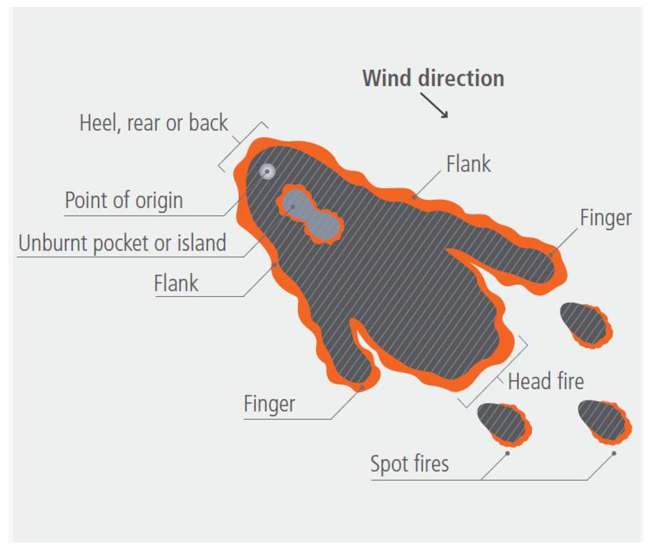
Landscape scale wildfire shapes have numerous components as illustrated in
Figure 1.
The forward
RoS and intensity of an active front of a fire, known as the head fire, is dependent on the fuel available for consumption in the active flaming front [
26,
27]. This is incorporated into existing empirical wildfire models [
2,
3] through the consideration of available fuels within a 1 ha assessment area, representative of the active fire area directly behind the head fire. Typically driven by wind direction, the head fire is the main component of a wildfire contributing to the
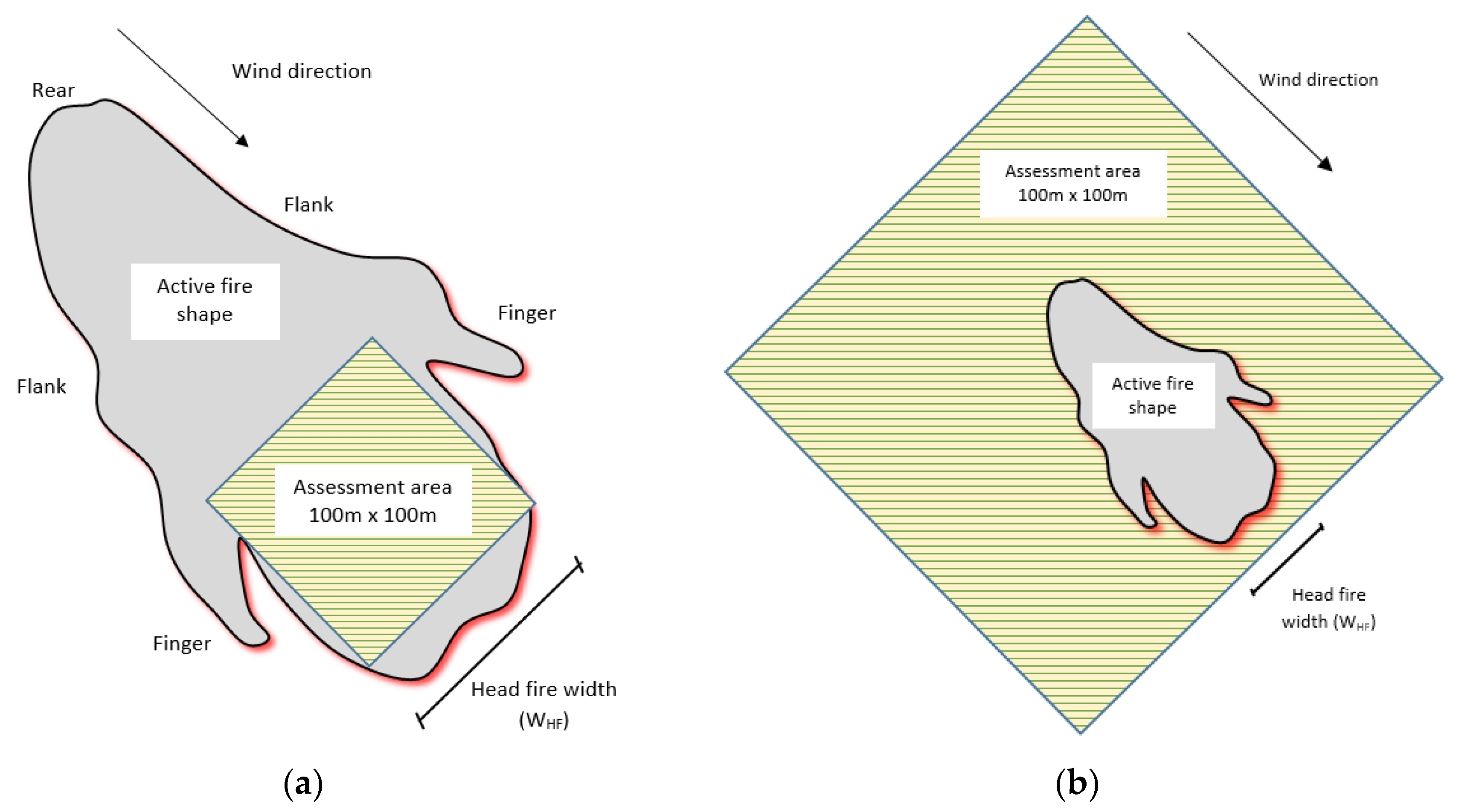
RoS and fire behaviour intensity. Subsequently, it is the focus when calculating radiant heat flux for the purposes of determining the appropriate standard of bushfire resilient residential construction. In landscape scale wildfire scenarios, the 1 ha area of assessment used for empirical models [
2,
3] falls within the greater active fire area, whilst in sub-landscape scale wildfire scenarios the active fire area instead falls within the 1 ha assessment area. This is illustrated in
Figure 2.
4. Modelling of Fuel Beds that Restrict Fire Growth
Within the urban environment, wildfire growth in road reserves, urban parklands, and similar scenarios can be restricted by the geometry of the available fuel beds. Current approaches of [
2,
3] suggest modification of the head fire width may be appropriate in these instances. However, whilst the width of the head fire is a vital component in determining radiant heat flux, head fire widths greater than 40 m resulted in negligible differences between the view factor and radiant heat flux within 30 m of the flame front [
4]. Through analysis of heat release rates, [
4] identified that reduction of head fire width alone without further consideration of fuel bed geometry was not suitable in scenarios where the fuel bed geometry restricted fire growth. Further, [
4] identified that:
Regardless of the actual geometry and coverage of fuel within the assessment area, [
2] assumes landscape scale wildfire behaviour with a 100% homogenous fuel loading within the assessment area and a head fire width of 100 m;
When fuel bed geometry prevents a 100 m head fire or quasi-steady RoS being obtained, failure to adjust wildfire fuel inputs may result in significant overestimation of wildfire impact, particularly radiant heat flux; and
In order to more accurately model wildfires in fuel beds that restrict fire growth, it is necessary to calculate available fuel loads that will contribute to fire behaviour over the area being assessed using the vegetation availability factor equation as described below.
Whilst the head fire flame width should be considered as the width of the continuous fuel contributing to the active fire front, the area covered by potential fuel load available for contribution to the
RoS and intensity of the active fire as a fraction of the total assessment area is defined as the vegetation availability factor (
VF), given by
where the fuel cell area is the coverage of vegetation present within a 100 m by 100 m assessment area directly in front of the receiving body. The available surface fuel load
wA (t/ha), and the available total fuel load
WA (t/ha), are then defined as
and
where
and
are respectively the surface fuel load and total fuel load sourced from relevant jurisdictional data sets.
The calculated fuel loads can then be applied to the relevant fire behaviour equations of RoS, fire line intensity, and flame length for the purposes of determining the suitability of wildfire fighting strategies and tactics or for calculating the radiant heat flux on receiving bodies in the path of the head fire. Where models do not consider the fuel load when calculating RoS, the vegetation availability factor can still be applied for the purposes of calculating radiant heat flux, fire line, and intensity.
5. Modelling Point Source Ignitions
In point source accelerating fire scenarios, whereby the developing fire originating from a single ignition point is yet to grow sufficiently to reach the quasi-steady
required to support the assumptions used in landscape scale wildfire behaviour, the accelerating head fire rate of spread
(km/h) in forest and woodland fuels is given by [
18,
28]:
where
is the equilibrium/potential head fire rate of spread (km/h),
t is the time since ignition (h), and
β (h
−1) is a constant related to how rapidly the head fire accelerates. Further, [
18,
28] suggest that a reasonable first estimate for
β can be established using the assumption that the fire will accelerate to 90% of the equilibrium rate of spread in 30 min (i.e., 0.5 h) for treed vegetation structures, including forest and woodlands. The attainment of the 90% equilibrium rate of spread 30 min post ignition within treed fuel structures is supported by the findings of [
17,
23,
28,
28].
Applying this to Equation (4) gives
and
t = 0.5, as illustrated below to solve the fire acceleration parameter (
):
It is worth noting that the value of
stated in [
18,
28] is in units of (min
−1). This would only be appropriate in the current setting if the
were considered in km/min rather than km/h.
For modelling purposes, the time since ignition may not be known, therefore the ability to determine the rate of spread of an accelerating fire in terms of distance travelled since ignition is required. As is the rate of change of distance D (km) with respect to time, it follows that
By integrating Equation (4) with respect to time, and setting D(0) = 0, the distance travelled post ignition can be expressed as:
From Equation (4) we know that
which when inserted this into Equation (5), enables distance travelled post ignition to be written as:
or alternatively as:
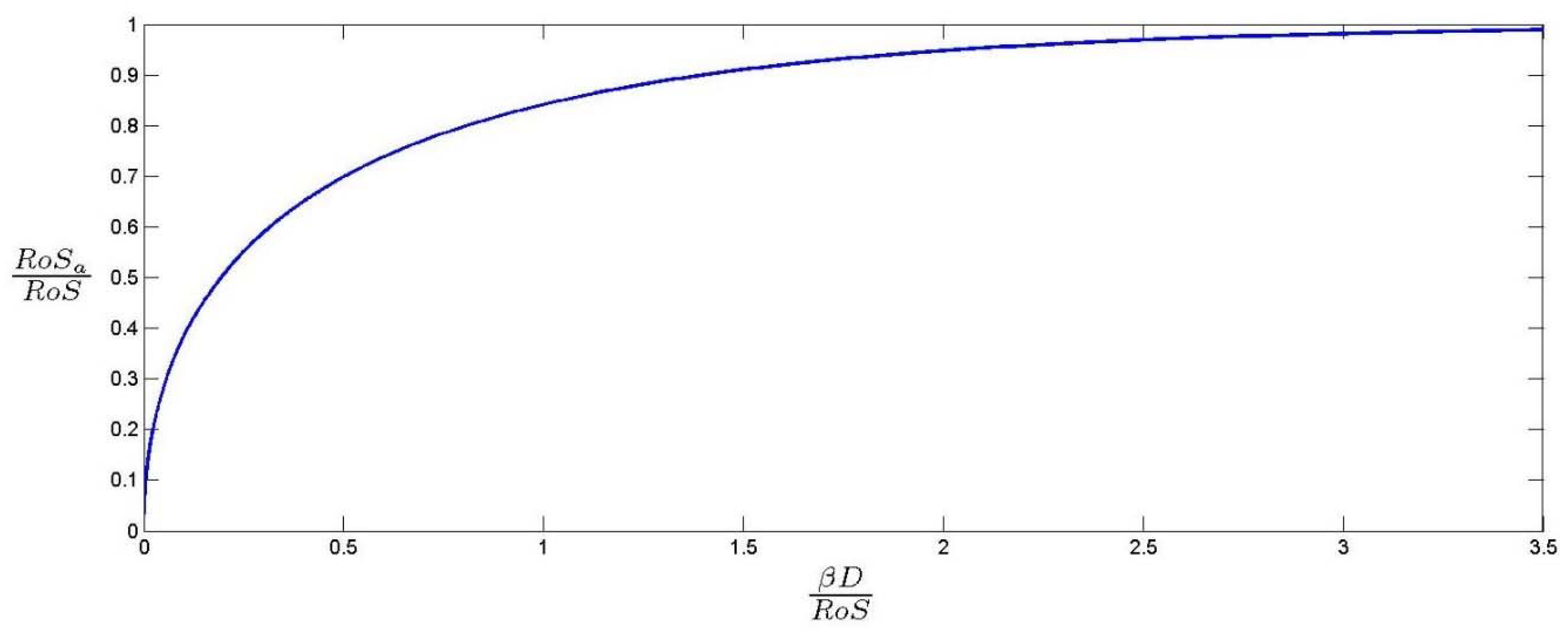
Equation (7) can be used to determine the
of an accelerating head fire
at a specified distance
D from the point source ignition with the equilibrium rate of spread. The problem is that it is not possible to re-arrange Equation (7) to express
as a function of
D. To resolve this issue a plot of
is numerically generated against
which can be used to approximate the ratio
(and hence
) for a given value of the ratio
. Such a plot is given in
Figure 3 below.
Once is calculated, it can be incorporated into the empirical modelling as demonstrated in Case Study 2, enabling greater accuracy in predicting impacts from small vegetation fires.
6. Modelling the Radiant Heat Flux of a Partially Shielded Fire Front
Within the urban environment, substantial non-combustible structures may stand between the receiving body and the fire front. For modelling purposes, it is assumed that these structures include significant walls or buildings, but not tin fencing or the like. Ignoring the impact of these structures on view factor, as is the case in [
2,
3], may result in over estimation of wildfire impacts. The radiant heat flux
q (kW/m
2) of a wildfire is calculated as the product of the flame emissive power
E (kW/m
2), the atmospheric transmissivity
, and the view factor
[
2,
3]. It is expressed as:
The flame emissive power (
E) is calculated using the equation:
where
is the Stefan-Boltzman constant,
is the flame emissivity, and
Tf is the flame temperature.
The view factor is a geometrical factor ranging from 0 to 1 which is related to the extent that the fire front fills the field of view looking from the site toward the flame. A value of indicates that the entire field of view consists of flame (i.e., not even sky), while a value of indicates that the fire front is completely out of view. As such, it is the view factor that must incorporate the impact of non-combustible obstructions on the radiant heat flux. To address this issue, this section proposes an alternate view factor model.
Calculation of the view factor in the wildfire context, detailed by current methods [
2,
3], is complex. In accordance with [
2,
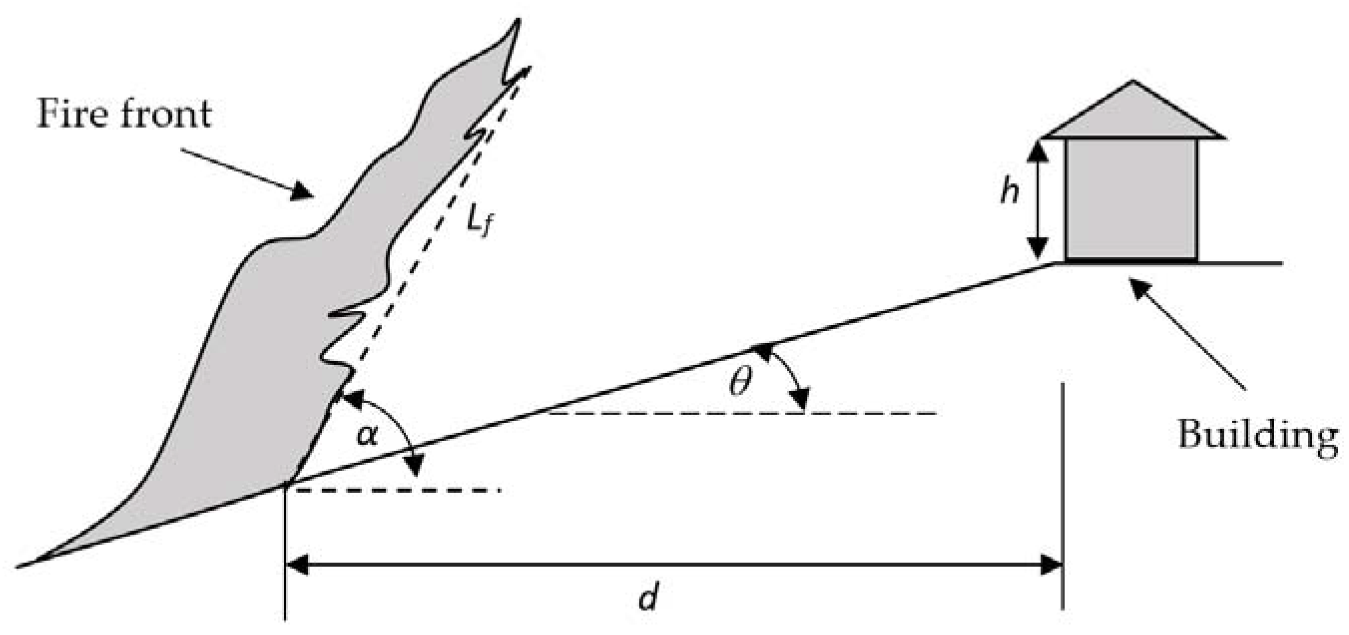
3] and referring to
Figure 4 below, the view factor calculation in the absence of shielding bodies is expressed as:
If
then
otherwise, if
then
where
is the flame length (m),
is the flame width/head fire width (m),
is the flame angle (degrees),
is the slope of the land between the site and vegetation fuel bed (degrees),
is the horizontal distance between the site and the vegetation fuel bed (m), and
is the elevation of the receiver (m).
Figure 4 provides an illustration of these variable in relation to a typical site and fire front. In order to consider the worst case scenario, the view factor is maximized with respect to the flame angle
. To do this, an optimization algorithm [
2,
3] is used.
In order to incorporate the impact of non-combustible obstructions, the total combined view factor of the obstructions must be calculated and then subtracted from the unobstructed view factor given by Equations (8)–(12). In describing the details of this approach, we generalise Equations (8)–(12) and re-write them as follows:
Equations (9) and (12) impose the assumption that the site is horizontally central with respect to the fire front. This assumption will be relaxed to allow the calculation of view factors for obstructions and fire fronts which are not centrally aligned to the site.
Equations (8)–(12) are formulated in terms of parameters specifically referencing the fire front (not an obstruction). Furthermore, although convenient from a computational perspective, they are not presented in a means that offers significant geometrical insight. The equations will be reformulated in terms of view angles from the site to the fire front or obstruction(s).
The first step of the proposed method is to generalise and amend the existing view factor model. The second step is to consider the effect of shielding obstructions.
6.1. Generalisation and Reformulation of the View Factor Formulae
To detail the alternate view factor model proposed, we will now discuss the geometry of approaching wildfires and the associated mathematical representation.
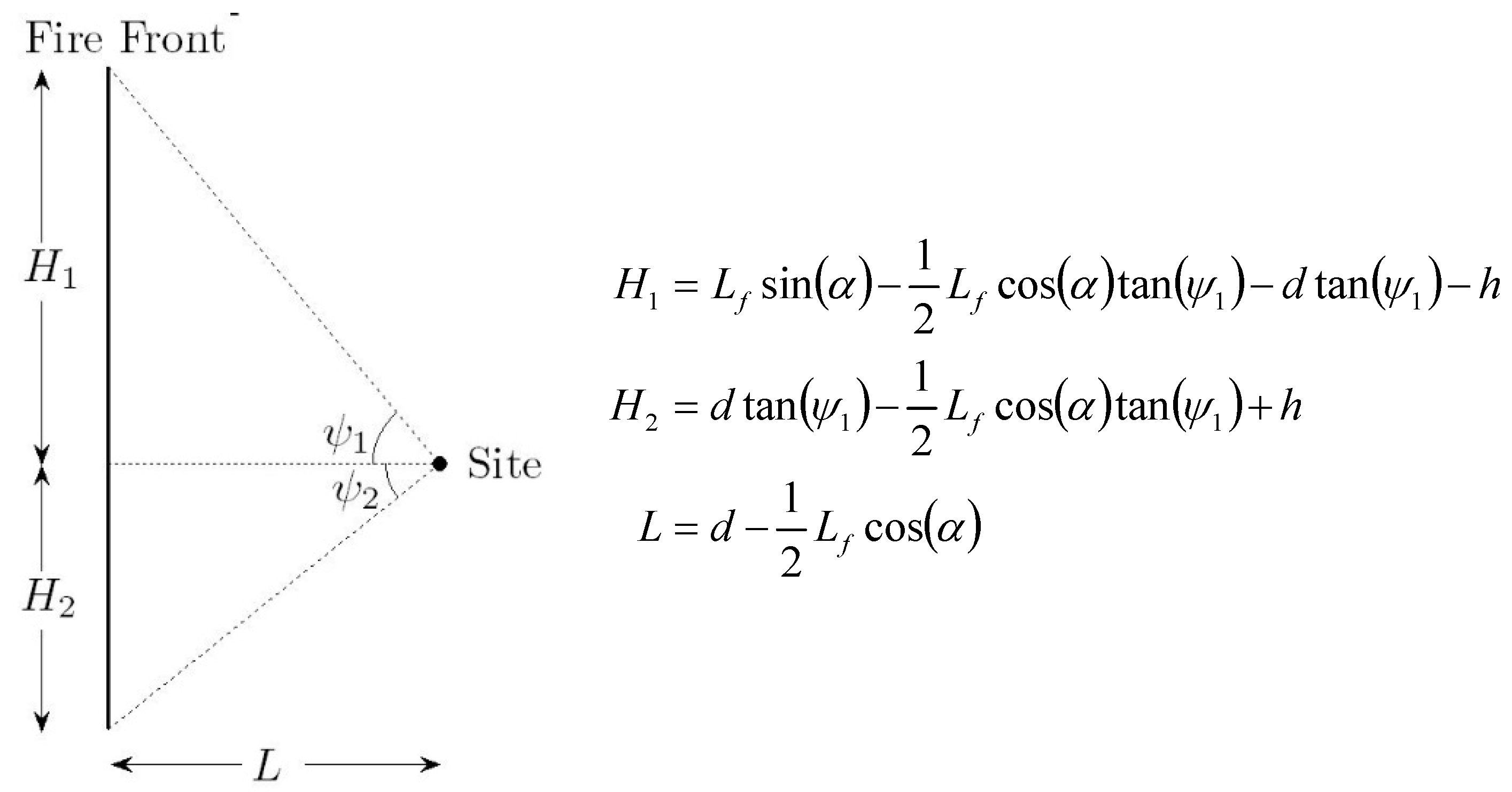
Figure 5 displays a generalised geometrical representation of the side view of a fire front and site. Consistent with the view factor calculation assumptions of [
2], an inclined flame is approximated by a vertical flame with the same height as the inclined flame (height measured vertically from the highest point of the flame to the ground directly below) and located in the middle of the inclined flame.
With reference to
Figure 5, and Equations (10) and (11), it becomes evident that:
for
i = 1,2.
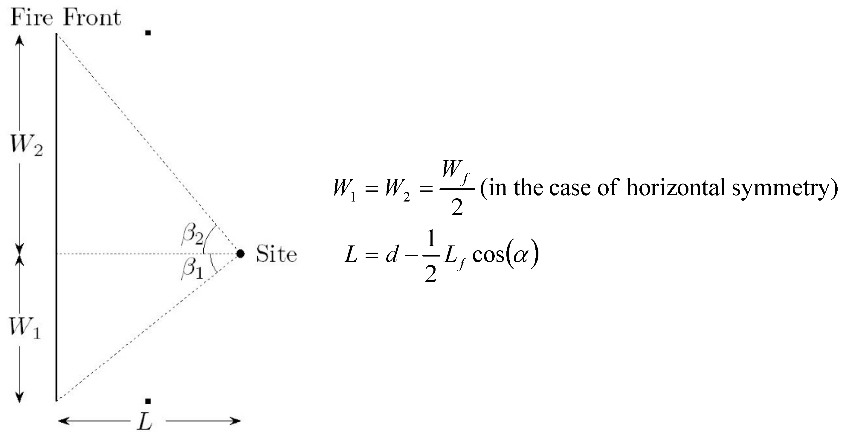
Figure 6 displays a generalised geometrical bird’s-eye view of the fire front and site. Equation (8) enforces the assumption that the site is horizontally central with respect to the fire front by setting
, however wildfires may not be centered with respect to the receiving structure. To reflect this,
Figure 6 represents a generalised asymmetrical case.
With reference to
Figure 6, and Equation (12), it becomes evident that:
for
.
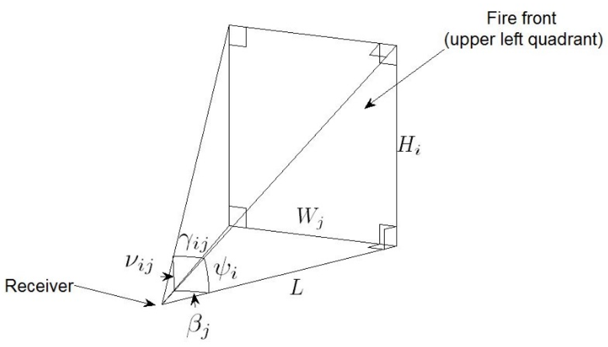
Figure 7 displays a three dimensional representation of the upper-left quadrant of the fire-front relative to the site, and the four angles
,
,
, and
,
,
. The indexing of quadrants is summarised in
Table 1.
With reference to
Figure 7, it becomes evident that:
for
. Accordingly, the generalised view factor for a rectangular approximation to a fire front or obstruction that does not pass through the site can be expressed as:
where the angles
,
,
, and
,
,
are as defined in
Figure 5,
Figure 6 and
Figure 7. Consistent with Equation (8), if the vertical approximation to the flame front lies on or behind the site (relative to the direction of travel of the fire front) the view factor is assigned the value
.
6.2. Calculating the View Factor Subject to Shielding Obstructions
The method for calculating the view factor of a flame front that is at least partially obstructed by non-combustible structures incorporates greater complexity than the existing model of [
2,
3], which do not consider the impact of obstructions on radiant heat flux. To assist with its discussion we describe it with reference to the
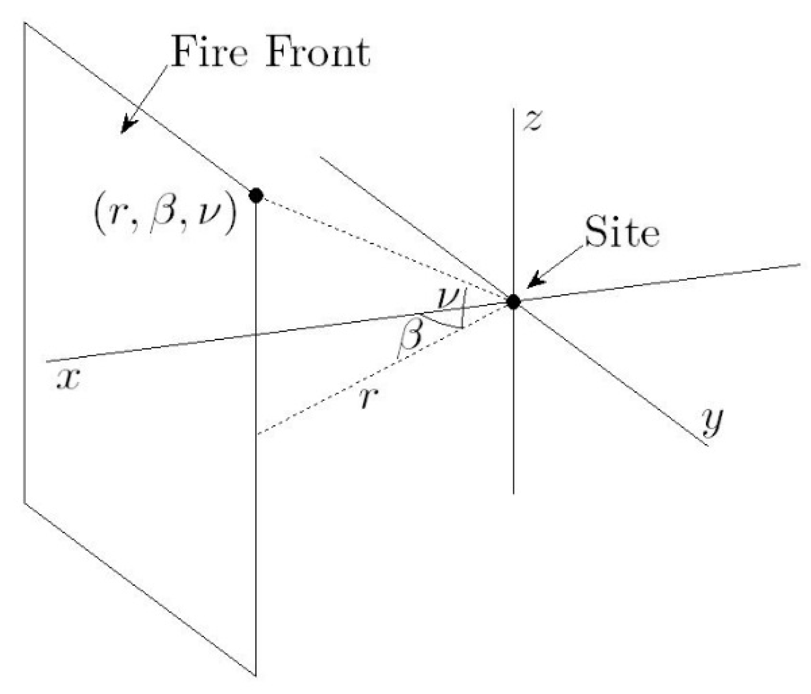
coordinate system illustrated in
Figure 8.
The component is the distance from the site measured in the − plane, is the angle in the − plane measured anticlockwise from the positive -axis when viewed from above (i.e., ), and is the vertical angle measured from the − plane with positive values for , and negative values for .
The view factor calculation method is based on a discretisation of the fire front with respect to
as illustrated in
Figure 9.
The discretisation consists of a total uniformly distributed values , with minimum value corresponding to the leftmost edge of the flame front (looking from above), and maximum value corresponding to the rightmost edge.
Consider the vertical rectangle illustrated in
Figure 10.
In order to calculate the view factor of the
Figure 10 rectangle using Equation (13), the angles are set as follows:
A single flame front with top edge coordinates denoted
and bottom edge coordinates denoted
is illustrated in
Figure 11.
We now consider a collection of
M obstructions with top edge coordinates denoted
and bottom edge coordinates denoted
for
. Note that
for
since the obstruction(s) may not span the full horizontal angular extent of the fire front when viewed from the site, and any part of an obstruction lying beyond the angular extent of the fire front does not impact the view factor calculation. This is illustrated in
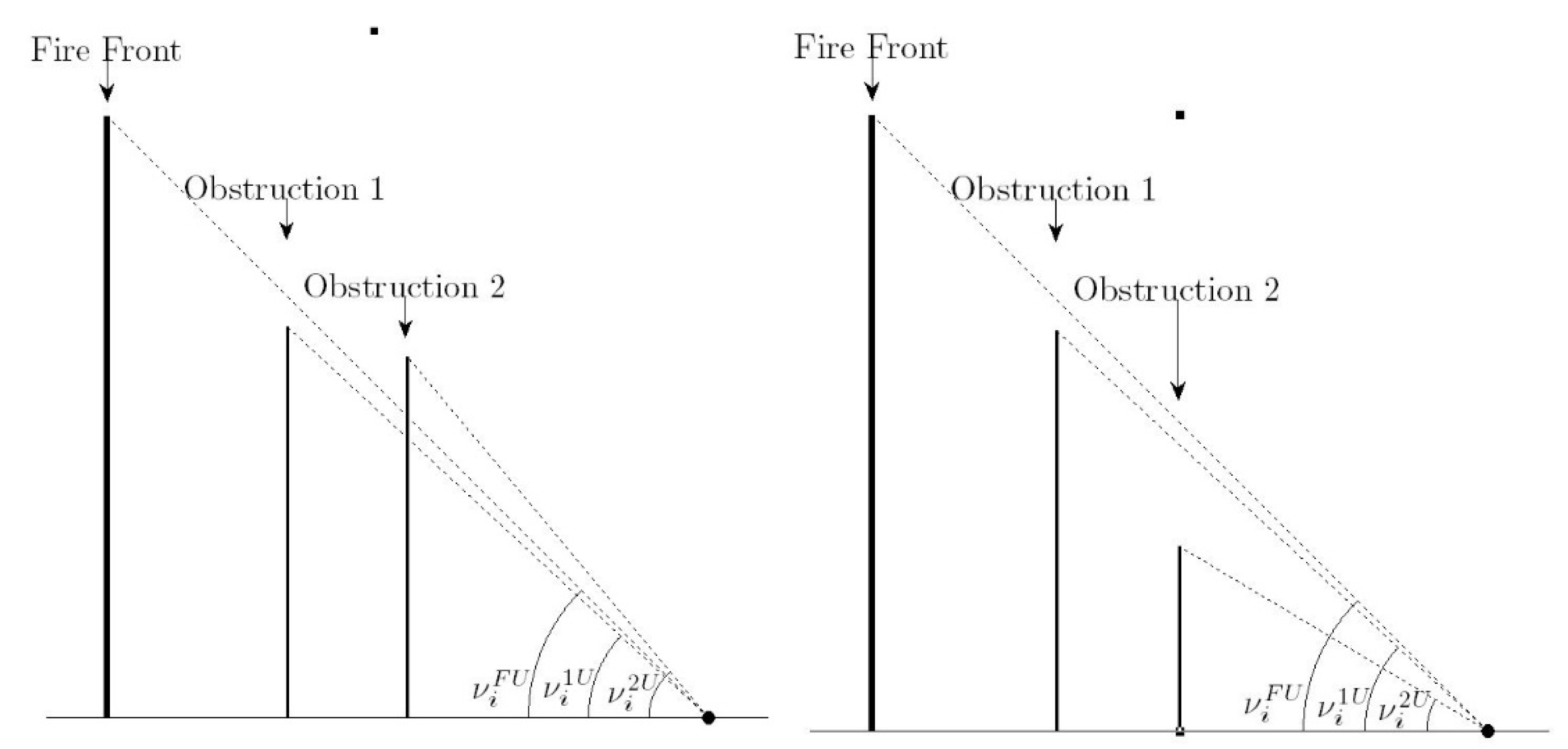
Figure 12.
The calculation of the view factor
subject to shielding obstructions proceeds as follows: If
(i.e., the center of the inclined flame is directly above or behind the site, so the vertical approximation to the fire front is on top of the site) then
otherwise
Calculate the view factor of the unobstructed vertical approximation to the fire front by setting , , and in Equation (14), and then substituting the resulting angles into Equation (13).
In order to accommodate non-rectangular obstructions, the obstructed view factor
is calculated by approximating the obstructions using thin rectangles defined within the angular increments from
to
for
. For each angular increment, the obstructed view factor
is calculated by determining the maximum value of
and minimum value of
for the obstructions that lie between the flame front and the site. If
, then
is used to denote the top of the obstructing rectangle, as any part of the obstruction extending above the flame front does not actual block the view of the flame front. This is illustrated in
Figure 13.
Similarly, if
, then
is used to denote the bottom of the obstructing rectangle. Denoting the angle to the top and bottom of the obstructing rectangle on increment
as
and
respectively, it follows that
where
The obstructing view factor for each angular increment is calculated by setting in Equation (14), and then substituting the resulting angles into Equation (13).
Calculate the total obstructed view factor
Calculate the view factor of the partially obstructed flame front
6.3. Modifications to the Optimisation Algorithm
In order to consider the worst case view factor with respect to the flame angle in this approach, four modifications need to be made to the optimisation algorithm of [
2,
3]:
In the original algorithm the initial value (lowest value) of the flame angle considered in the optimisation algorithm is the site slope
. This is not a valid angle in the case that an obstruction exists between the flame front and the site, as it effectively allows the fire front to penetrate the obstruction. To avoid this situation it is necessary to set the initial flame angle such that the fire front would clear the obstruction. This amounts to setting
when
. Note that
denotes the site slope, and
and
denote the maximum height and
component of obstruction
at angle
relative to the site.
A further complication could arise if the center of the fire front lies in front of the obstruction when the base of the fire front lies behind the obstruction. The issue in this instance is that the obstruction would not have an impact on the view factor. To avoid this situation the minimum flame angle is required to satisfy
when
. Note that
is the flame length, and
is a small positive number (e.g., 10
−6).
If the fire front is positioned on top of an obstruction, the flame angle is set to 90 degrees to effectively consider the fire front as being behind the obstruction. In this case, the algorithm is not required to proceed further to determine an optimal value of .
Since the algorithm does not start with the flame angle
equal to the site slope
, it is possible that the initial value of
could turn out to be the flame angle that optimises the view factor. The standard optimisation algorithm of [
2,
3] terminates or refines its search increment when the view factors
,
, and
, which correspond to the flame angles
satisfy
and
, however, if
at the first step the algorithm will not terminate. Hence the additional termination or refinement criteria,
must be added to the algorithm in addition to the existing criteria (i.e., (
and
) or
).
In the case that the obstruction completely obscures the line of sight from the building site to the top of the flame front, the optimisation algorithm will never terminate as it will not be able to identify a non-zero view factor no matter how much the flame angle () is increased. In order to avoid this situation, an additional condition is added to both loops of the algorithm. Specifically, if ° during the iteration then the algorithm will terminate immediately, and the flame angle will be set to °. This measure is only required to avoid an infinite loop, and will not affect the outcome of the calculation.
7. Case Studies
A number of case studies are presented to illustrate the application and implications of the approaches described previously to consider radiant heat flux from a fire front while accounting for fuel loading, non-combustible obstruction(s), or accelerating fire fronts.
7.1. Case Study 1
The first case study considers a semi-rural environment in which a row of single and two story brick houses backs onto forest type bush land with a fuel bed of unrestricted geometry and
Vf = 1. Suppose that the radiant heat flux of a fire in the bush land behind the houses is to be estimated at a site or house on the opposite side of the street. The geometry of the specific case considered here is provided in
Figure 14.
The parameter values used in the calculation as described in [
2] are summarised in
Table 2.
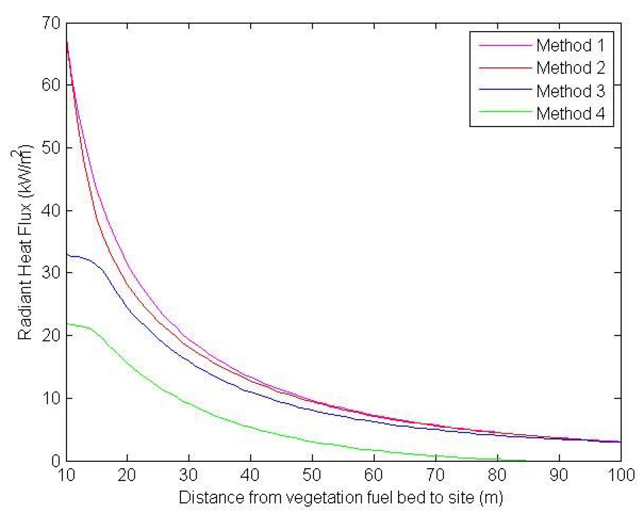
The radiant heat flux was calculated for a range of distances from the site to the vegetation fuel bed ranging from 10 m to 100 m. For the sake of comparison, the radiant heat flux at the site was estimated using four calculation methods:
The method outlined in [
2], ignoring the obstructions presented by the houses located between the site and vegetation fuel bed.
The method outlined in [
2] with the receiver height
set to 3 m (instead of the mid-level of the flame front).
The method outlined in this paper, where each of the four houses is considered to reduce the view factor of the flame front.
A simplified method in which the four obstructions are considered as a single rectangular obstruction with height 5 m (i.e., the height of the tallest house), and width equal to the combined width of the four houses. The combined width is the distance from the westernmost edge of the westernmost structure to the easternmost edge of the easternmost structure.
Figure 15 provides a plot of the radiant heat flux at the site as a function of the distance to the vegetation fuel bed using each of the methods 1–4 outlined above.
As expected, the methods that did not consider the shielding effect of the houses (magenta and red lines) provided higher estimates for the radiant heat flux compared to the methods that did consider the shielding effect (blue and green). For small distances to the vegetation fuel bed, the approaches that did not consider shielding significantly over-estimated the radiant heat flux compared to the method presented in this paper (blue line). As the distance to the vegetation fuel bed increases, the difference between the [
2] approach and shielding approach presented here becomes small. This is most likely because the 10 m gap between house 2 and 3 becomes the most significant zone for heat flux for a more distant fire front, so the impact of the obstructions becomes less significant.
Method 4 (green line) provided the lowest estimates of radiant heat flux as expected. As the distance to the vegetation fuel bed increased, the radiant heat flux estimated using this approach tended to zero far more rapidly than the other methods. This was most likely due to the significant gap between house 2 and house 3, which was not blocked in methods 1–3, but was blocked when the four houses were approximated as a single rectangular obstruction. This highlights the importance of considering multiple obstructions individually to ensure that the impact of radiation through significant gaps is not diminished.
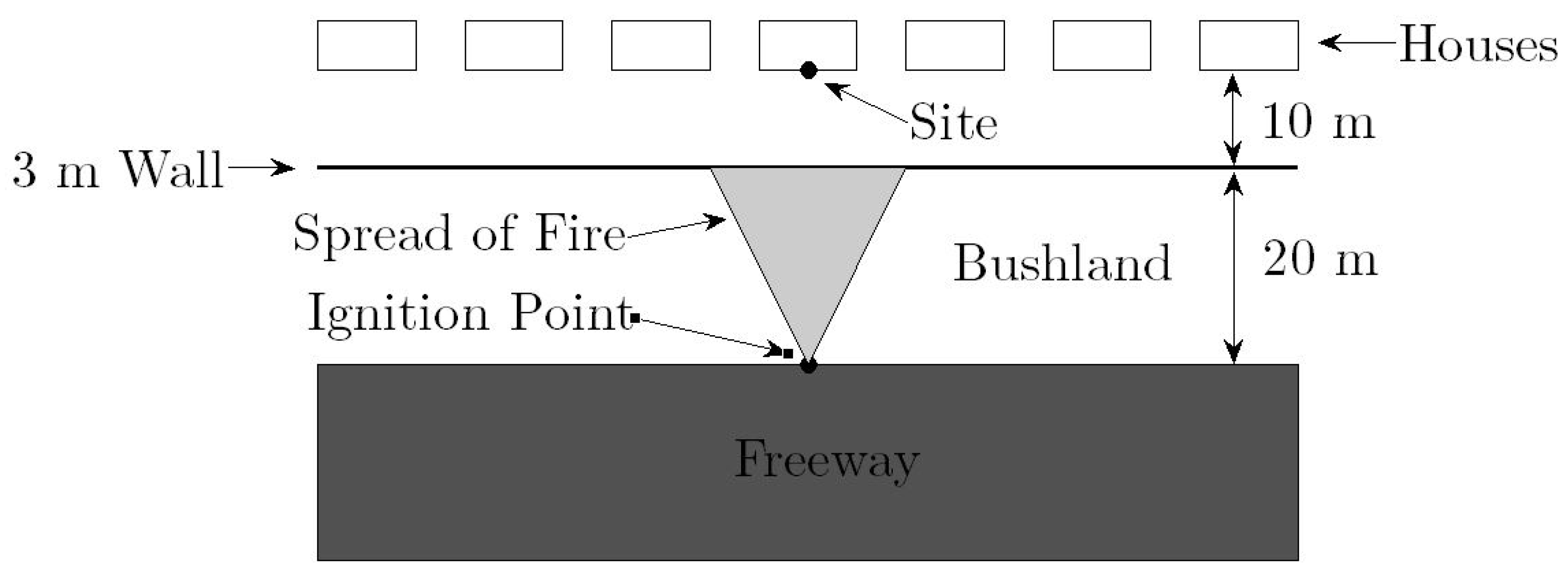
7.2. Case Study 2
The second case study considers an accelerating fire front burning within a 20 m wide treed forest style bushland zone within the road reserve between the edge of a freeway or highway and a 3 m brick wall separating the freeway from housing. The geometry of the vegetation fuel bed prevents the fire attaining its maximum potential rate of spread. There is a row of houses located 10 m on the other side of the brick wall, one of which will be considered the site at which the radiant heat flux from the fire will be considered. The geometry of the specific case considered here is provided in
Figure 16.
The parameters used in the calculation are summarised in
Table 2. In addition, the vegetation factor
Vf = 0.2 scales back the surface and overall fuel loads as defined in Equations (2) and (3). The fire is assumed to ignite from a point source at the edge of the Freeway, 30 m from the site/receiver. The fire is assumed to spread perpendicular to the Freeway at an accelerating rate
, which is related to the distance from the ignition point
D by Equation (7). The rate parameter
h
−1, as suggested by [
18,
28], is utilised.
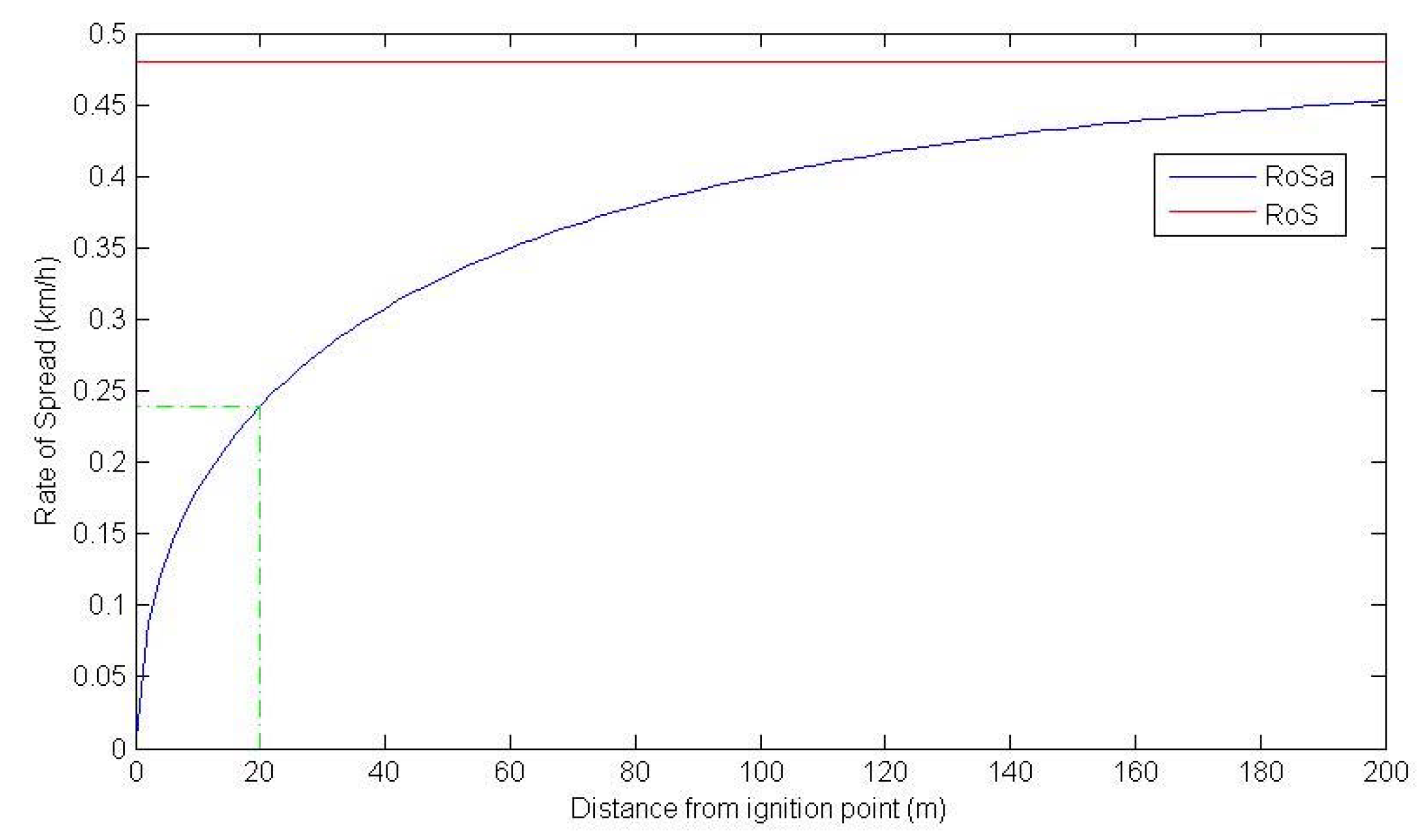
Figure 17 provides a plot of the accelerating rate of spread
and the equilibrium rate of spread
against the distance from the ignition point
D.
From
Figure 17 it is apparent that over 20 m (i.e., the distance from the ignition point to the obstructing wall) the rate of spread reaches approximately half of its equilibrium value. The rate of spread perpendicular to the forward direction is assumed to be half the forward rate of spread, so the flame width is given by
.
The impact of incorporating the acceleration of a fire front and an obstruction into the heat flux model has been highlighted by comparing the above scenario with an additional seven modelling variants. The eight scenarios are summarised as follows:
The fire front is modelled with a constant (equilibrium) rate of spread from the ignition point, a width of 100 m, a vegetation factor of
Vf = 1, and the obstruction (wall) is ignored (the model of [
2]).
The fire front is modelled with a constant (equilibrium) rate of spread from the ignition point, a width of 100 m, a vegetation factor of Vf = 0.2, and the obstruction (wall) is ignored.
The fire front is modelled with an accelerating rate of spread from the ignition point, a vegetation factor of Vf = 1, and the obstruction (wall) is ignored.
The fire front is modelled with an accelerating rate of spread from the ignition point, a vegetation factor of Vf = 0.2, and the obstruction (wall) is ignored.
The fire front is modelled with a constant (equilibrium) rate of spread from the ignition point, a width of 100 m, a vegetation factor of Vf = 1, and the obstruction (wall) is included.
The fire front is modelled with a constant (equilibrium) rate of spread from the ignition point, a width of 100 m, a vegetation factor of Vf = 0.2, and the obstruction (wall) is included.
The fire front is modelled with an accelerating rate of spread from the ignition point, a vegetation factor of Vf = 1, and the obstruction (wall) is included.
The fire front is modelled with an accelerating rate of spread from the ignition point, a vegetation factor of Vf = 0.2, and the obstruction (wall) is included (i.e., the Case Study 2 scenario).
The radiant heat flux for the above scenarios are plotted against the distance from the site in
Figure 18 and
Figure 19.
As expected, the heat fluxes when the wall is ignored are all greater than the corresponding fluxes when the wall is incorporated into the model to provide shielding. Furthermore, the fluxes with
Vf = 1 exceeded those with
Vf = 0.2. All of the models that include the modelling of acceleration start from a flux of zero, which increases as the rate of spread, length, and width increase (in addition to the increase from the larger view factor as the front closes on the site). Significantly, in
Figure 19 the yellow line corresponding to the Case Study 2 scenario is not visible as the heat flux at the site remains zero. This is because the fuel load and rate of spread are not sufficient to create a front with sufficient height to be visible above the 3 m obstruction after 20 m of spreading, with the flame height reaching only 2.4 m.
The progression of the flame front over the bush region between the freeway and obstructing wall is illustrated in
Figure 20 for scenarios 5 to 8.
The model of [
2,
3], which assumes the wildfire is established and has attained a quasi-steady rate of spread, estimates the time taken for the ignited fire to travel from the freeway to the wall (20 m) is 30 s, while the model incorporating the acceleration of the spreading front and the reduced vegetation density estimates the time at 9 min, consistent with the findings of [
4,
18,
23].
8. Discussion
The case studies presented in the previous section indicate potential significant over-estimation of radiant heat flux using the approach outlined in [
2,
3] in cases involving non-combustible obstructions and point-source ignition fires for a minimum of 20 m separation from the fire front. This is significant as it is in this distance that wildfire flame radiation is considered to have its greatest impact [
22,
30]. Such situations are common in urban environments. The results demonstrate the importance of appropriately considering fuel geometry, wildfire behaviour, and the effect of shielding structures when calculating radiant heat impacts on buildings and emergency responders within urban environments where vegetation fuel bed geometry prevents wildfires reaching landscape proportions.
Over estimation of potential radiant heat flux impacts could, in turn, result in:
Firefighters not being deployed to suppress wildfires and defend homes as a result of over-estimation of wildfire behaviour that indicates suppression efforts are not suitable, resulting in avoidable house loss and impacts on communities. This may occur as firefighting suppression thresholds are related to wildfire behaviour parameters throughout jurisdictions internationally [
31]. Where inappropriate predictions fail to consider vegetation geometry that does not support the assumptions of landscape wildfire modelling, otherwise defendable areas may be left unguarded due inappropriate evaluation of suppression strategies;
Inappropriate modelling of wildfire through landscaped gardens, public open space, road reserves, and residential areas within urban areas. In turn, land that is actually suitable for development may be identified as being subject to overestimated wildfire impact which restricts or prohibits development altogether. Typically, this may occur in urban settings where a small unmanaged vacant residential lot is modelled as supporting a landscape scale wildfire, in turn restricting or prohibiting development on adjacent and near-by lots; and
Unnecessary requirements for over engineering and wildfire resistant construction standards of affected dwellings and structures that hinders development through either misidentification of land as being subject to unacceptable levels of wildfire impact, or through making development cost-prohibitive as a result of the level of wildfire resistant engineering and construction required.
In addition to the inherent safety factor incorporated within the vegetation availability factor previously discussed, the methodologies proposed also retain the assumption of a flame emissivity ε = 0.95, being representative of a landscape scale wildfire with an active uniform flame front depth greater than 2 m, and even potentially greater than 10 m [
20,
24]. In cases where the active flame front will not reach this depth, it may also be suitable to reduce the emissivity. It is important to note that whilst the vegetation factor and modified view factor model are applicable to all fuel types (forest, woodland, shrub, scrub, grassland, etc.), the point source acceleration model presented in this paper is suitable for treed forest and woodland structures only, as fire growth in other fuel structures may be significantly faster.
There are several alternate existing methods [
30,
31,
32,
33,
34,
35,
36] that propose various solutions to calculating radiant heat flux and other wildfire impacts on the urban environment. However, unlike the models presented in this paper, none are suitable for direct application into the adopted approaches of [
2,
3], nor do they provide detailed construction standards required to increase resilience to the calculated level of wildfire impact. Even [
32], which reports to have the potential to revolutionise heat flux evaluation methods, currently remains a next generation product that cannot be applied at this point in time to resolve the shortfalls identified in this paper. A benefit of the acceleration model provided in this paper is that it can be used to predict the impacts of potential spotting in urban areas by treating each fire as a new point source ignition. In this manner, the effect of the accelerating RoS is considered, something that is ignored in [
33], which models radiant heat flux from cylindrical shaped discrete landscape tree fires.
The models presented in this paper are not intended to address the potential radiant heat flux arising from surrounding buildings being involved in fire. In part, this is inherently considered within [
2,
3] through the requirement that associated structures on the same parcel of land and within 6 m of the dwelling subject to enhanced construction standards, must also be constructed to that same standard. In new estates, all dwellings within the land development should be constructed to the required standard of wildfire resistance, significantly reducing the potential for mass conflagration spreading between multiple houses in theory. Where radiant heat flux between buildings is required to be calculated, [
33] proposes an incident radiant heat transfer model which may be utilised. Due to the differences in wildfire and structural fire behaviour and radiation models [
2,
3,
4,
6,
7,
8,
9,
10,
11,
19,
20,
21,
22,
23,
24,
25,
26,
27,
30,
32,
33,
34,
35,
36,
37] as well as the difference in building and structure performance once impacted by wildfire [
38,
39], it is suggested that a high level of technical expertise is required to complete this process. One limitation of both existing methodologies and the methodology presented in this paper is the assumption that wildfire impacts occur perpendicular or ‘front on’ to the receiver. One avenue for future work is to establish methodologies for calculating the radiant heat flux as a result of flanking fires, whereby the head fire front passes parallel to the receiving body.
When considering the suitability of fire suppression strategies, there are factors other than radiant heat flux that also require consideration. Whilst these are not addressed in this paper, current research into firefighter tenability [
31] and critical flow rates required for wildfire suppression [
40] may in part address this issue.


