Spatially-Resolved Spectroscopic Diagnostics of a Miniature RF Atmospheric Pressure Plasma Jet in Argon Open to Ambient Air

Abstract

The spatially-resolved electron temperature, rotational temperature, and number density of the two metastable Ar $1s$ levels were investigated in a miniature RF Ar glow discharge jet at atmospheric pressure. The $1s$ level population densities were determined from optical absorption spectroscopy (OAS) measurements assuming a Voigt profile for the plasma emission and a Gaussian profile for the lamp emission. As for the electron temperature, it was deduced from the comparison of the measured Ar $2p_i\to 1s_j$ emission lines with those simulated using a collisional-radiative model. The Ar $1s$ level population higher than 10${}^{18}$ m${}^{-3}$ and electron temperature around 2.5 eV were obtained close to the nozzle exit. In addition, both values decreased steadily along the discharge axis. Rotational temperatures determined from OH(A) and N${}_2$(C) optical emission featured a large difference with the gas temperature found from a thermocouple; a feature ascribed to the population of emitting OH and N${}_2$ states by energy transfer reactions involving the Ar $1s$ levels.

1. Introduction

Understanding non-thermal atmospheric-pressure plasma sources is of increasing interest for a wide range of industrial and biomedical applications as they can provide plasma chemistry without low-pressure conditions [1,2,3]. As an example for biomedical applications, the electron temperature needs to be hot enough to produce reactive species, whereas the neutral gas temperature has to stay near room temperature to avoid excessive heating of the tissues. Over the years, a number of configurations for sustaining non-thermal plasmas at atmospheric pressure have been developed, mainly in the form of dielectric barrier discharges (DBDs), micro-discharge jets, and glow discharges generated in confined space [4,5,6,7,8,9]. A key advantage of the atmospheric pressure plasma jet (APPJ) is the ability to transport various reactive species to a region separated from the plasma generation zone [10,11,12]. This spatial separation allows objects spanning a wide range of sizes and shapes to be treated, especially for biomedical, surface treatment, and plasma chemical functionalization applications [13,14,15].

In order to implement these plasma sources as viable options, advanced diagnostics are needed to characterize and optimize their processing efficiency under various operating conditions (e.g., power, gas flow rate, choice of feed gas and precursor, etc.). In this context, various APPJs have been developed and characterized in the past two decades [16,17,18]. Currently, stable jet devices can operate with various electrical excitations (DC, pulsed DC, kilohertz frequency AC, radio-frequency (RF), and microwave), and in many different gases, from noble gases, to diatomic gases, to air. Depending on the electrical excitation and the jet geometry, different plasma characteristics can be selected for the application of interest. Some jet devices are able to generate radicals over very large distances [19] or can be bundled together to cover a larger surface [20].

Recently, Léveillé et al. [21] designed an APPJ with a hollowed electrode to produce a stable discharge in an inert gas and added an injection source of reactive species downstream of the plasma-forming zone. Such a device is well suited for atomic species and radical production and transport for precise bio-applications such as the treatment of skin tissues and cells. Some studies showed, using nanosecond camera imaging, that the jet was formed by fast moving ionization volumes, often called “plasma bullets”, and that the bullet velocity and diameter increased with the applied voltage [22,23]. Laser diagnostics have been applied to obtain more insight into the plasma chemistry, e.g., the concentration and behaviour of OH radicals and O atoms [24,25].

Although huge improvements have been made in the fundamental understanding of plasma jets, important plasma characteristics such as the metastable and resonant population density of Ar atoms and electron temperature are still under investigation for most configurations. Moreover, highly populated Ar $1s$ states (Paschen notation) are suspected to play a major role in the chemistry of the flowing afterglow (such as molecule fragmentation) due to the large portion of energy they carry [26,27]. Therefore, accurate information on the spatial distribution of the Ar $1s$ level population is highly required to understand the underlying physics and chemistry of APPJs operated in Ar.

In this work, optical emission spectroscopy (OES) and optical absorption spectroscopy (OAS) are used on an APPJ operating with Ar and open to ambient air. The neutral gas temperature profile is estimated using computational fluid dynamic (CFD) calculations considering a 2D-axisymmetric representation of the APPJ. These simulations also allow the observation of the basic flow pattern, as well as the mixing of the jet with the surrounding air. The spatially-resolved metastable ($1s_3$, $1s_5$) population density of Ar atoms is estimated from OAS measurements, performed with a standard low-pressure Ar lamp. Using the estimated gas temperatures and the measured values of the population of metastable Ar atoms, a collisional-radiative model along with OES measurements of Ar $2p$-to-$1s$ transitions is used to estimate the spatial distribution of the electron temperature (T${}_e$).

2. Experimental Setup and Methods

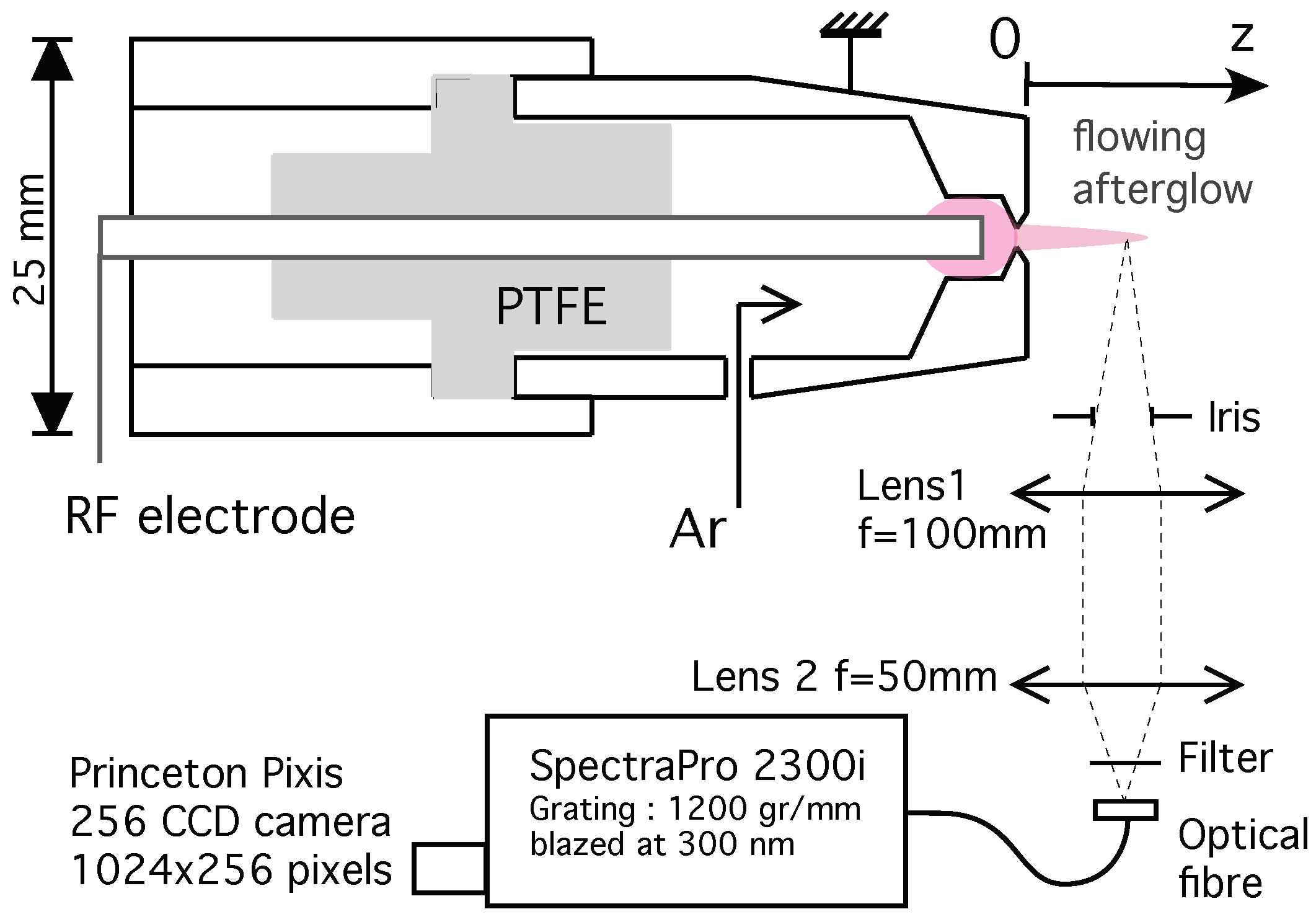
2.1. Setup Configuration

The non-thermal atmospheric pressure plasma jet (APPJ) was produced using a device similar to, but larger than, the original design of Léveillé and Coulombe [21]. A schematic is shown in Figure 1. The coaxial geometry device featured an RF-powered capillary electrode at the centre, surrounded by a grounded nozzle, both parts being insulated by a PTFE spacer. The device diameter was 2.5 cm, and the nozzle exit diameter was 1 mm. The plasmagen gas was injected in the ring formed by the two coaxial electrodes. The capillary electrode allowed injection of a secondary gas in the flowing afterglow discharge. The grounded outer electrode was made of stainless steel, while the inner capillary electrode, adjustable in the axial position, was made of brass. This electrode was held in place by an O-ring located between two compressed PTFE sleeves. Argon was used with a flow rate of 5 standard litres per minute (slm). The RF power, set at 40 W, was delivered from a 13.56 MHz 300 W generator (Cesar Generator Model 1312 Advanced Energy) equipped with an automatic matching network (Dressler VM1000 A). Consequently, ∼90% (∼36 W) was absorbed by the plasma. The discharge formed inside the nozzle throat, and the flowing afterglow streaming into the surrounding atmosphere formed the jet.

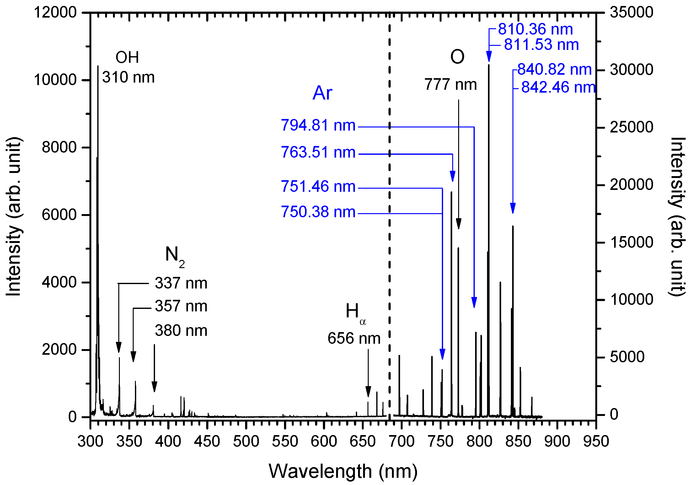
2.2. Optical Emission Spectroscopy

Optical emission spectroscopy (OES) measurements were performed using a spectrometer (Princeton Instruments Acton SpectraPro2300) equipped with a CCD camera (Princeton Instruments PIXIS 1024×256). The 25 cm focal length combined with a 1200 lines/mm grating, blazed at 300 nm, provided a spectral resolution of 0.22 nm (full width at half maximum) at $\lambda$ = 632 nm. The light emitted by the discharge region was collected using a confocal microscope system with two lenses with f = 50 mm and 100 mm, respectively (Figure 1). With this optical setup, the magnification was 0.5. A 200 μm-diameter optical fibre, located at the focal point of the imaging lens, was connected to the entrance slit of the spectrometer. Considering the magnification, the spatial resolution was 400 μm.

Light was collected from the centre of the plasma jet, perpendicular to the discharge axis, and all the recorded spectra were corrected for the spectral response of the optical fibre, monochromator, and detector. All spectra were averaged over many cycles of the applied RF power (integration times of tens of milliseconds), and a typical example is presented in Figure 2. Strong Ar-I emission lines were observed in the 700–900 nm wavelength range. Besides these anticipated Ar lines, noticeable emissions from N${}_2$ (second positive system), N${}_2^{+}$ (first negative system), OH (A-X), O-I (777 nm), and H-I (656.3 nm) were also observed. These were due to the interaction of the APPJ with ambient air.

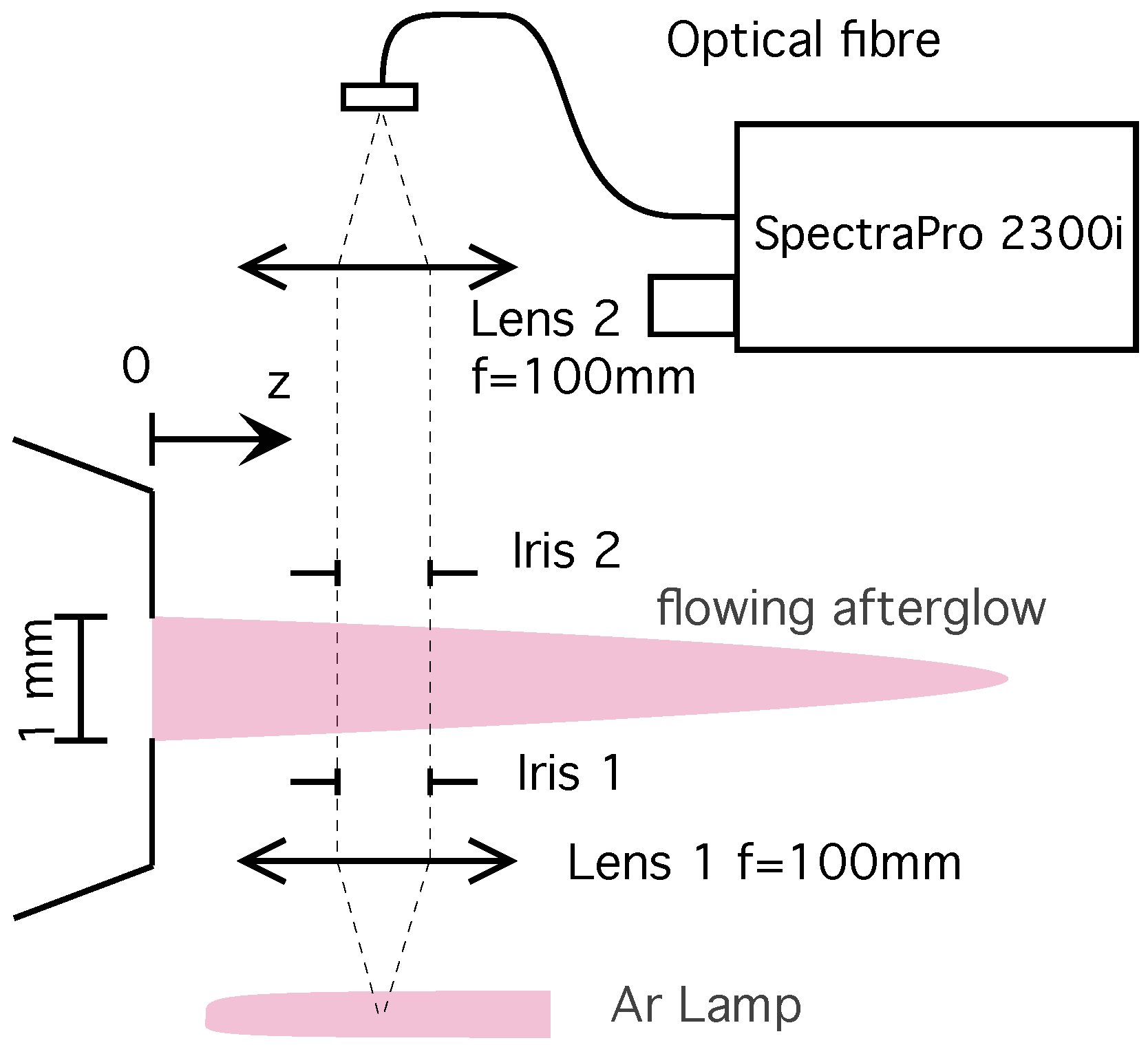
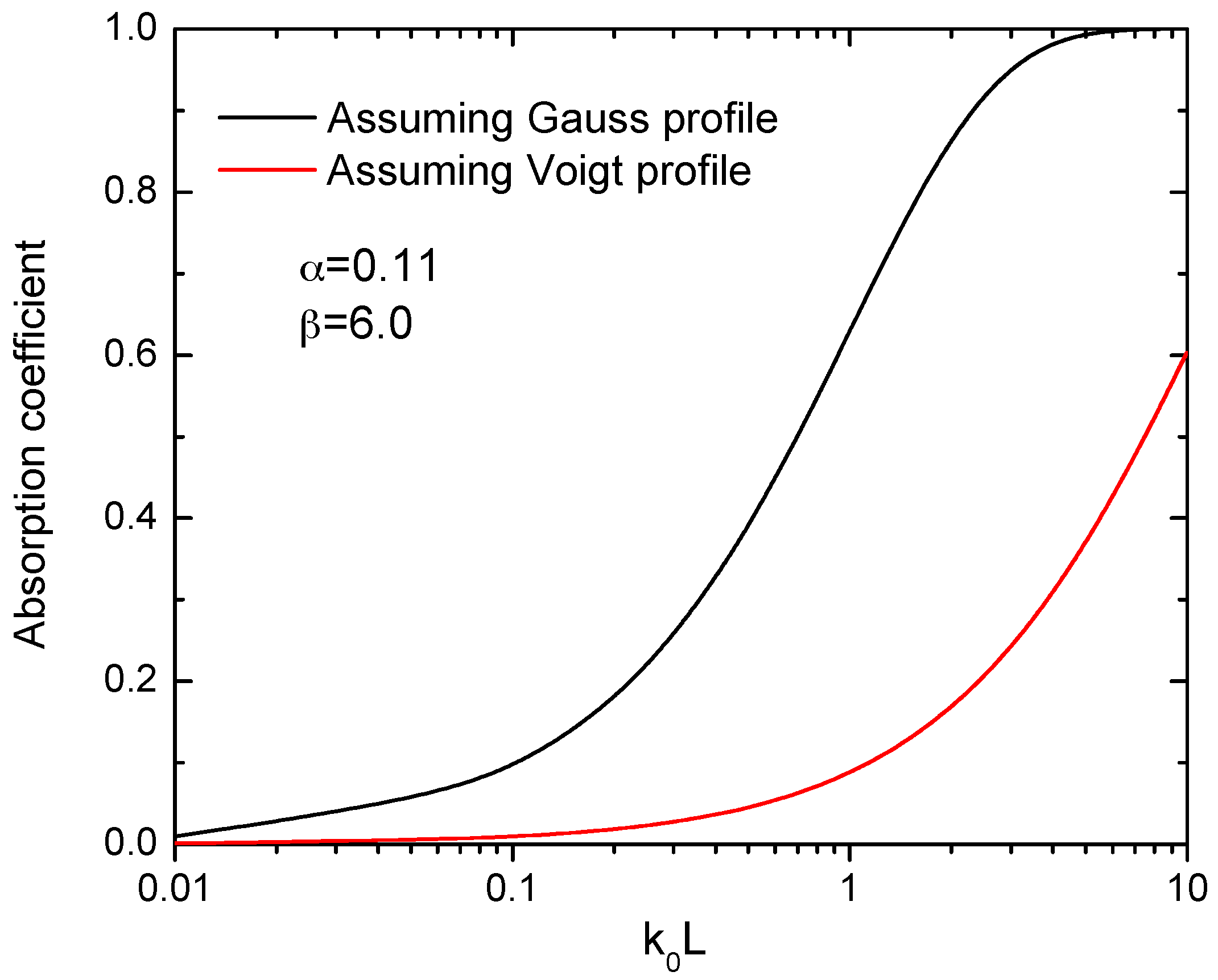
2.3. Optical Absorption Spectroscopy

Optical absorption spectroscopy (OAS) measurements were in part performed using the same spectrometer, but with a different light collection arrangement. A schematic of the absorption setup is presented in Figure 3. The light emitted by the low-pressure argon spectral lamp (Philips) was collimated by a first lens (f = 100 mm) and then went through a first iris to ensure that a parallel beam with a well-controlled diameter (0.5 mm) was obtained. Next, the beam passed through the plasma jet, a second iris, and a second lens (f = 100 mm) before finally reaching the optical fibre.

Using this experimental setup, the global optical absorption coefficient, $A_L$, can be obtained from:

$$A_L=1-\frac{I_{p+l}-I_p}{I_l}$$

(1)

where $I_{p+l}$ is the emission of the plasma with the lamp on, $I_p$ is the emission of the plasma with the lamp off, and $I_l$ is the emission of the lamp with the plasma off. The analysis method was then adopted from Castaños-Martinez and Moisan [28] to take into account the difference in pressure broadening between the low-pressure Ar lamp and the atmospheric-pressure Ar plasma. This method assumed a Voigt line profile to carry out the analysis, thus taking into account the pressure broadening of the Ar emission lines from the plasma. As a result, the frequency-integrated absorption coefficient for each individual line can be expressed as [28]:

$$A_L=\frac{\int e^{-{\left(\frac{\omega }{\alpha }\right)}^2}\left(1-e^{-k_{0}L\frac{\beta }{\pi }{\int }_{-\infty }^{\infty }\frac{e^{-y^2}dy}{{\beta }^2+{(\omega -y)}^2}}\right)d\omega }{\int e^{-{\left(\frac{\omega }{\alpha }\right)}^2}d\omega }$$

(2)

which depends on the central frequency absorption coefficient $\left(k_0\right)$ and the absorption length (L). The frequency integration occurs through the variable $\omega$:

$$\omega =\frac{2(\nu -{\nu }_0)}{\Delta {\nu }_D}\sqrt{\ln 2}$$

(3)

where ${\nu }_0$ is the central frequency of the transition and $\Delta {\nu }_D$ the Doppler half-width component of the line broadening. The $\alpha$ and $\beta$ coefficients are defined as:

$$\begin{array}{c}\hfill \alpha =\frac{\Delta {\nu }_D\left(\mathrm{lamp}\right)}{\Delta {\nu }_L\left(\mathrm{plasma}\right)/2+\sqrt{{(\Delta {\nu }_L\left(\mathrm{plasma}\right)/2)}^2+\Delta {\nu }_D^2\left(\mathrm{plasma}\right)}},\end{array}$$

(4)

$$\begin{array}{c}\hfill \beta =\frac{\Delta {\nu }_L\left(\mathrm{plasma}\right)}{\Delta {\nu }_D\left(\mathrm{plasma}\right)}\sqrt{\ln 2}\end{array}$$

(5)

with $\Delta {\nu }_L$ the Lorentzian half-width component. The Doppler half-width was calculated according to $\Delta {\nu }_D=7.16\times {10}^{-7}{\nu }_0\sqrt{T_g/M}$, where $T_g$ is the gas temperature and M is the atom mass (in atomic units). This equation allowed the calculation of the plasma Doppler broadening at each position when taking the neutral gas temperature obtained from CFD simulations (detailed in Section 3.1). As for the lamp Doppler broadening, it was calculated by estimating a temperature of 600 K as suggested by Moussounda [29]. Afterwards, the Lorentzian half width $\Delta {\nu }_L$ was obtained again at each position by deconvoluting the Voigt profile of the measured plasma emission lines. To measure with enough precision the broadenings of these emission lines and those of the Ar lamp used for the OAS analysis, a very good spectral resolution was required. For that set of experiments, light was sent via an optical fibre to the entrance slit of a HORIBA Jobin-Yvon THR-1000 monochromator having a focal length of 1 m and a holographic grating of 1800 lines/mm. The exit slit was fitted with a Hamamatsu R-955 photomultiplier tube linked to a pico-ammeter. The spectral resolution was 0.05 nm at $\lambda$ = 632 nm.

Using the resulting $\alpha$ and $\beta$ values from this procedure, $A_L$ could be obtained for every position as a function of $k_{0}L$. In order to highlight the fact that, in our plasma conditions, the pressure broadening was significant, the $A_L$ values assuming a Gaussian profile are also plotted at the same spatial position (z = 0, nozzle exit) in Figure 4. It shows that, for given $A_L$ and L values, the assumption of a Gaussian profile would have underestimated the $k_0$ value and therefore resulted in lower population densities.

Finally, the absorption length of the APPJ was estimated by scanning the averaged absorption of the 751.5 nm line in the plane perpendicular to the jet axis. This profile was then fitted with a Gauss profile, as presented in Figure 5. The full-width at half-maximum (FWHM) of the fit being 0.6 mm, we used an absorption length of 1.2 mm.

Hence, by calculating $A_L$ from Equation (2) and using Figure 4 to see at which $k_{0}L$ this absorption would occur enabled us to extract the value of $k_0$. This value was then used in Equation (6) to find the population density of the lower level involved in the considered emission line:

$$N_i=\frac{4}{\sqrt{ln2}}\frac{g_i}{g_j}\frac{\Delta {\nu }_D}{{\lambda }_{ji}^2{A}_{ji}}\frac{k_{0}L}{L}\beta \int \int \frac{e^{-y^2}dy}{{\beta }^2+{(\omega -y)}^2}d\omega$$

(6)

The statistical weight ($g_j,g_i$) and the spontaneous decay coefficients $A_{ji}$ were obtained from the NIST database [30].

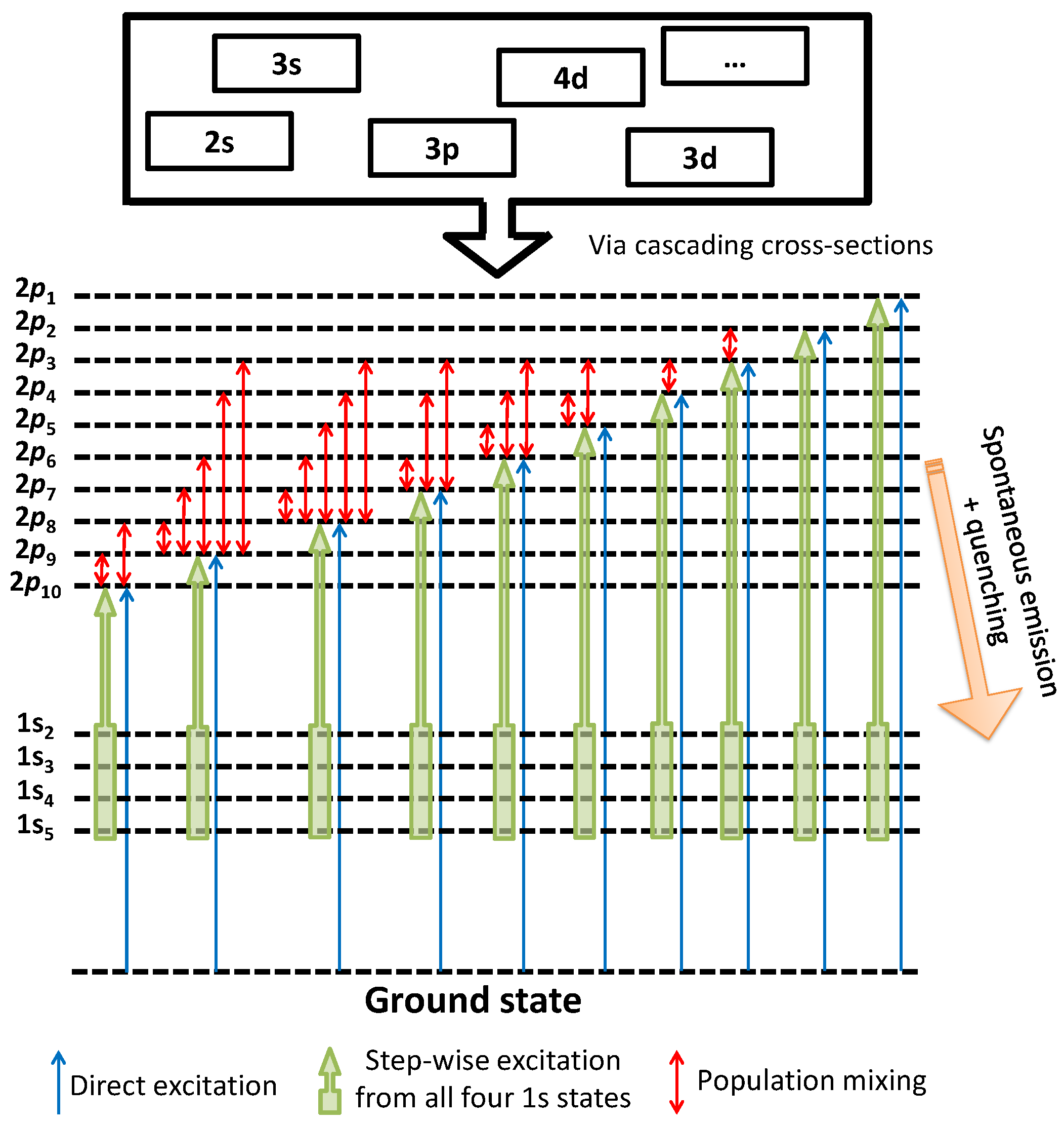
2.4. Collisional Radiative Model

In order to extract the electron temperature $T_e$ along the discharge axis, the measured Ar $2p_j$-to-$1s_i$ emission line intensities as seen in Figure 2 were compared to those predicted by a collisional radiative (CR) model solving the balance equations of the ten $2p$ levels assuming a Maxwell–Boltzmann electron energy distribution function (EEDF) and the steady state. As such, our approach to find $T_e$ was based on fitting the experimental spectra with theoretical ones instead of solely relying on an auto-coherent CR model. The details of this method can be found elsewhere [31]; only an overview is presented in the following lines.

The intensity of a given Ar I line emanating from a $2p_i$ level is given by:

$$I_{\lambda }=f\left(\lambda \right)A_{ij}{n}_i{\theta }_{ij}$$

(7)

where $f\left(\lambda \right)$ is the optical response of the optical fibre, monochromator, and detector, ${\theta }_{ij}$ is the escape factor, $A_{ij}$ is the Einstein coefficient for spontaneous emission (taken from the NIST database [30]), and $n_i$ is the number density of the Ar $2p$ state emitting at wavelength $\lambda$.

The role of the CR model is to find the optimal $n_i$ and ${\theta }_{ij}$ values by solving for a given number of $T_e$ values the particle balance equations for the 10 $2p$ levels. By comparing up to 24 emission lines from the experimental spectrum to all the simulated ones, a relative standard error calculation was done to evaluate the goodness of the fit [32]. For each experimental spectrum, the $T_e$ value yielding the most accurate simulated spectrum was assumed to be the actual electron temperature. The input parameters found from other diagnostics were the gas temperature, working pressure, plasma length along the line of sight of spectroscopic measurements, and the number density of Ar $1s$ levels. Since OAS measurements performed in this work only provided information about the $1s_3$ and $1s_5$ levels, two CR simulations were made for each spectrum assuming the Boltzmann equilibrium of the $1s$ levels: the first by imposing the $1s_3$ number density and the second by imposing the $1s_5$ number density. The mean $T_e$ value obtained from those two simulations was considered as the actual $T_e$, and the standard deviation provided the error bars.

Figure 6 summarizes the different mechanisms that were considered in the particle balance equations. Excitation mechanisms included electron impact from either ground or $1s$ metastable and resonant states, population mixing between two $2p$ levels induced by a collision with the ground state Ar atoms [33], as well as radiation trapping [31]. As represented by the box on top of Figure 6, apparent (cascading) cross-sections for electron collisions were used to calculate the corresponding reaction rates, thus ensuring that cascading effects were adequately described without going through the complexity of solving the population of energy levels higher than the $2p$. Furthermore, de-excitation mechanisms include radiative decay [30], quenching by neutrals [34,35], impurities [36], and again population mixing. In our case, we considered the impurities to be nitrogen and oxygen due to the interaction with ambient air (80% N${}_2$, 20% O${}_2$), and their concentrations along the plasma jet axis were deduced from the CFD simulations (see the details below). Radiation trapping and collisions involving neutrals made the CR model especially suited for non-equilibrium atmospheric-pressure plasma conditions, and population mixing by electrons was neglected because their density was assumed to be many orders of magnitude lower than the ground state Ar density.

Based on this framework, the coupled steady state particle balance equations of the $2p_i$ levels can be expressed as:

$$n_{2p_i}=\frac{\left(k_{Gi}{n}_G+{\sum }_{j=2}^5{k}_{1s_{ji}}{n}_{1s_j}\right)n_e+{\sum }_{j=1(j\ne i)}^{10}{k}_{2p_{ji}}{n}_G{n}_{2p_j}}{{\sum }_{j=1(j\ne i)}^{10}{k}_{2p_{ij}}{n}_G+{\sum }_{j=2}^5{A}_{ij}{\theta }_{ij}+k_{{Quench}_{Ar}}{n}_G+{\sum }_{Im}{k}_{{Quench}_{Im}}{n}_{Im}}$$

(8)

In Equation (8), $k_{Gi}$ denotes the reaction rate of the electron excitation from the ground state; $k_{1s_{ji}}$ the step-wise electron excitation from $1s$ levels; $k_{2p_{ji}}$ and $k_{2p_{ij}}$ the population mixing among the $2p$ manifold; $k_{{Quench}_x}$ the quenching coefficients by neutral argon atoms and impurities; and $n_{Im}$ the number density of impurities. Considering that the electron density $n_e$ is in every term of the numerator (indeed, it is also hidden in the $n_{2p_j}$ number density), it only acts as a scaling factor for the $2p$ number densities. Therefore, since only the relative emission line intensities (and thus the relative $2p$ number densities) were required for the model, the simulations were in fact independent of the electron density.

3. Results and Discussion

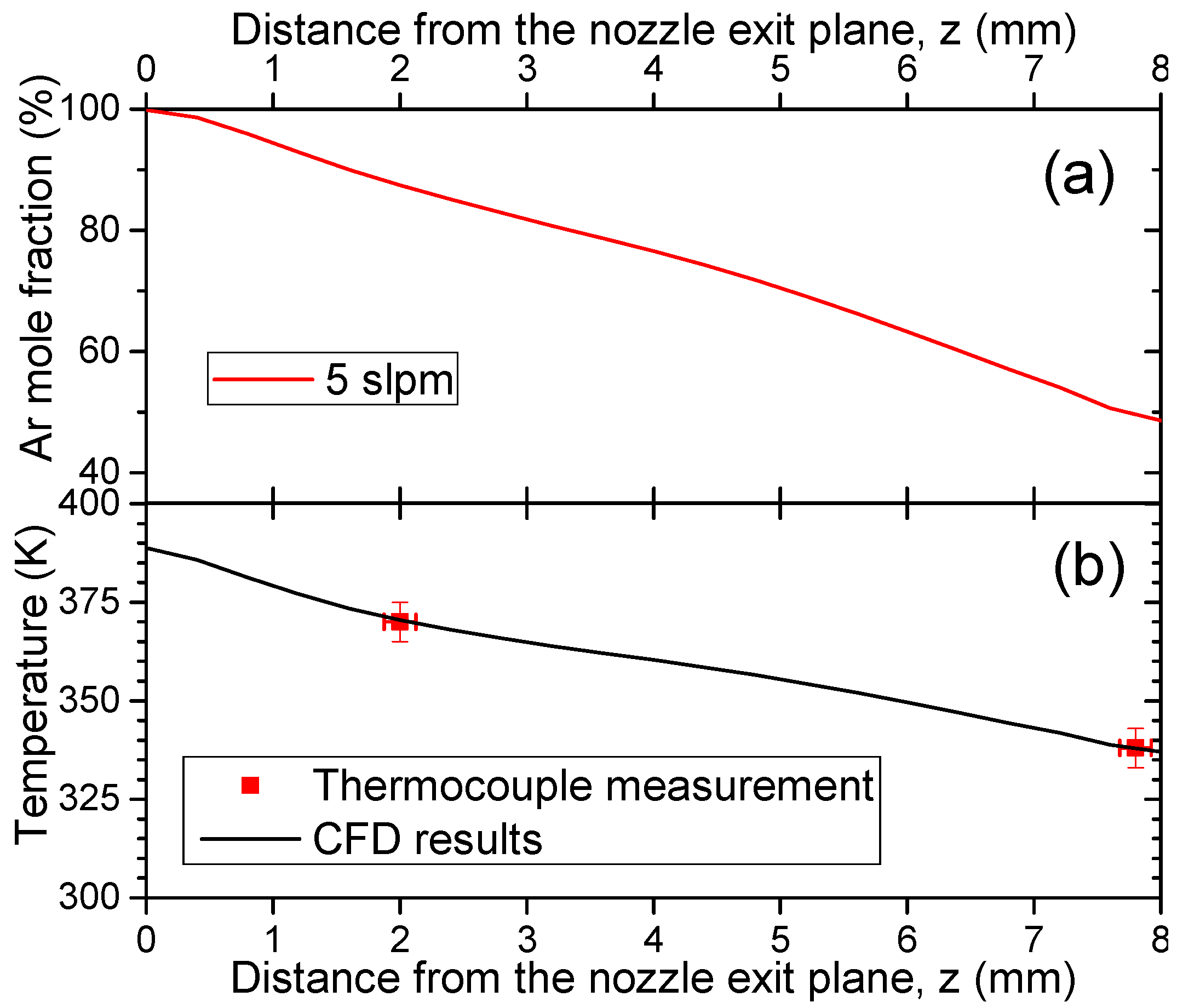
3.1. Gas Temperature and Fluid Flow

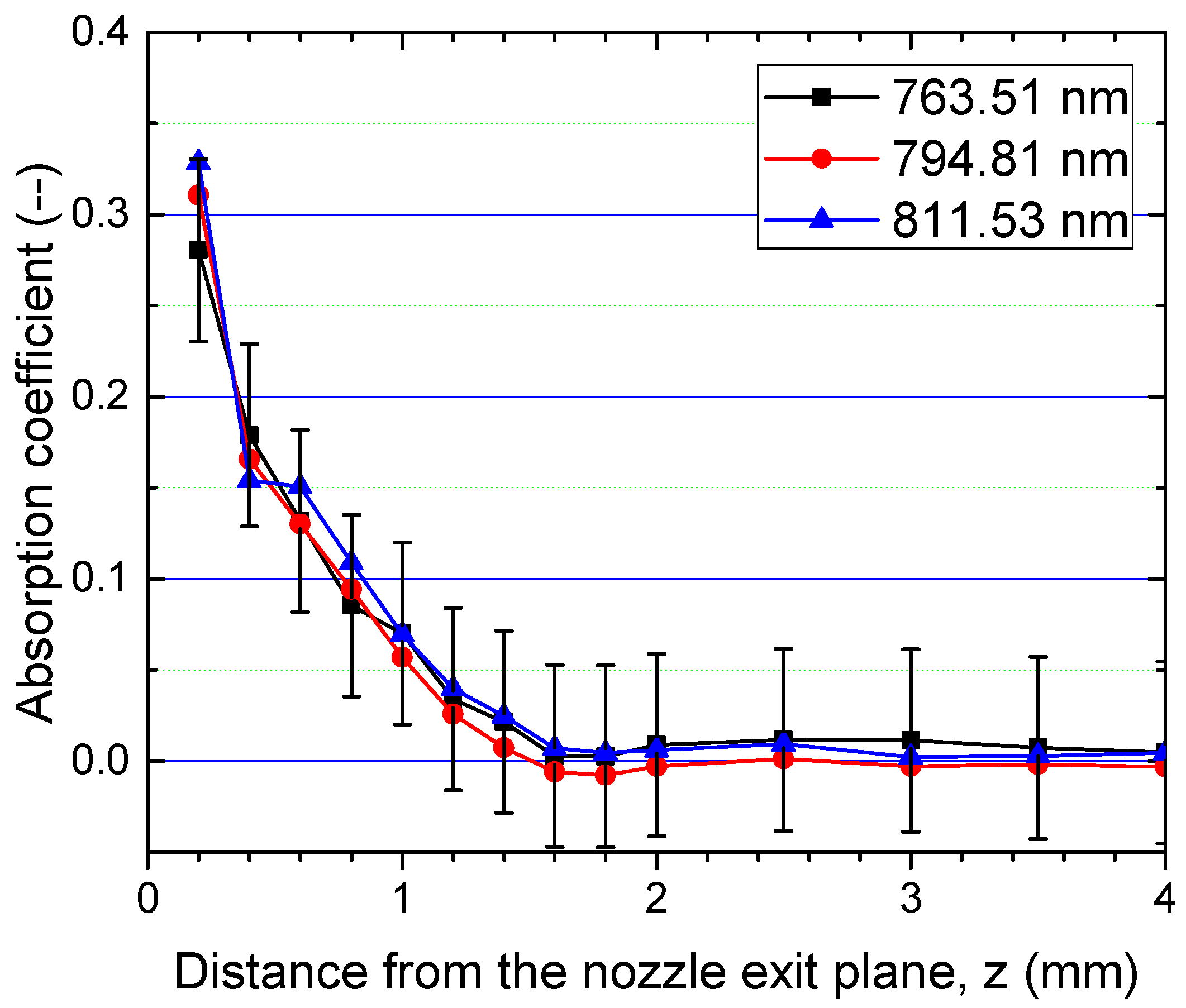
To ensure compatibility with temperature-sensitive applications, the plasma jet temperature profile was monitored. A first estimate was made using the OH and N${}_2$ rotational band emissions acquired with the OES setup over the 300-400 nm range. The observed transitions are the second positive system of nitrogen (N${}_2$(C${}^3{\mathsf{\Pi }}_u$) → N${}_2$(B${}^3{\mathsf{\Pi }}_g$), $\Delta \nu$ = 1, 2, 3) and the OH transition (OH(A) →OH(X)). The Specair software [37,38] was used to model the experimental OES results and to determine the corresponding rotational temperature. The results, presented in Figure 7, show a rotational temperature ranging from 500 to 1000 K, both for OH(A) and N${}_2$(C). In this figure, the z = 0 mm position is defined as the nozzle exit plane of the APPJ.

These temperatures were compared with a 1 mm RF-shielded thermocouple placed in the plasma jet. The gas temperature measured by the thermocouple ranged from 75 to 50 ${}^{\circ }\mathrm{C}$, 2 to 8 mm away from the outlet. Thus, OH(A) and N${}_2$(C) molecules featured much higher temperatures; this discrepancy most likely resulted from energy transfer collisions with the Ar $1s$ states [39]. Indeed, the energy of these levels was close to the excitation energy levels of OH(A) and N${}_2$(C), and as will be shown later, their density turned out to be relatively high.

In order to enhance our understanding of the APPJ investigated, its fluid flow was simulated with the commercial CFD code ANSYS Fluent v.14.5 [40]. Because of the cylindrical symmetry of the APPJ, a two-dimensional $r-z$ computational geometry was used. The geometry included the entire device, as well as an extended area (8 mm in z after the nozzle exit plane and 8 mm in r) for the analysis of the effect of surrounding air on the plasma jet. The plasma formation was not simulated in this preliminary study. To take into account neutral gas heating by the plasma on the flow pattern, the injection temperature of the argon was set to the temperature of the APPJ metallic nozzle, measured with the thermocouple, 390 K.

The combined incompressible Navier–Stokes and non-reactive species transport equations were solved in the 2D computational domain composed of 80,000 control volumes. As turbulence can be present due to the two geometry expansions adopted for this design, a standard k-epsilon model was used [41]. The number density of the argon-air mixture was calculated with the ideal gas equation. The boundary conditions were the imposed mass flow rate of argon at the inlet, the non-slip conditions at the walls, and atmospheric static pressure at the extended area boundaries.

From the CFD modelling results, Figure 8a shows the axial distribution of the argon mole fraction along the jet axis. It is shown that the argon mole fraction decreased due to the diffusion of the surrounding air into the jet. The 4 mm axial position composition was about a 25% mole air fraction. In theses conditions, and considering that the APPJ was pointing down, the flow was laminar.

Additionally, the CFD modelling results included the temperature evolution along the centerline. As shown in Figure 8b, the axial distribution of the gas temperature along the jet axis as predicted by the model was in very good agreement with thermocouple measurements at 2 and 8 mm.

3.2. Spatially-Resolved Ar $1s$ Level Populations

A typical absorption profile for a few of the most visible Ar lines is presented in Figure 9. The spatial step size was fixed at 0.2 mm, even though the spatial averaging was set by the iris opening of 0.5 mm. The corresponding horizontal error bars are omitted for clarity. With a flow rate of 5slm, the jet visually appeared to be ∼4 mm long, but for distances larger than 2.5 mm, the absorption coefficient was too low to be significant and thus used in the calculations.

Using Equation (6), the spatial distribution of the population densities of both metastable levels ($1s_3$ and $1s_5$) was determined. The results are presented in Figure 10. The population of excited states at the exit of the nozzle were found to be ∼7 × 10${}^{17}$ m${}^{-3}$ for $1s_3$ and ∼2 × 10${}^{18}$ m${}^{-3}$ for $1s_5$. Not surprisingly, the $1s_5$ number density was higher than the $1s_3$ one, and both densities decreased along the discharge axis (they were already two orders of magnitude lower 2 mm away from the nozzle exit plane).

Similar experiments were conducted by other research groups to study the Ar excited states, mainly using diode laser absorption spectroscopy. Niermann et al. [42] reported maximum densities of ∼1 × 10${}^{19}$ m${}^{-3}$ for the $1s_5$ level, which was one order of magnitude higher than our values. Additional experimental results were reported, but for Ar/He mixtures, with typically 1–5% Ar. Ar $1s_5$ level densities of ∼1 × 10${}^{16}$ m${}^{-3}$ [43] and ∼1 × 10${}^{17}$ m${}^{-3}$ were found [44]. However, no experimental measurements have been reported for the other three Ar $1s$ levels.

Recently, the behaviour of resonant and metastable levels of Ar was studied by Van Gaens and Bogaerts [36] who performed a kinetic modelling study. The power level reported was 6.5 W with an Ar flow of 2 L/min (compared to 40 W at 5 L/min in our experiment). These values provided roughly a factor of two lower power density compared to the present study. It was reasonable to compare the population predicted by the model to our measurement if the exit velocity of the gas was scaled: 29 m/s in the model and 150 m/s in the experiment. The populations of excited states reported at the exit of the nozzle were ∼10${}^{18}$ m${}^{-3}$ for $1s_5$ and ∼10${}^{17}$ m${}^{-3}$ for $1s_3$; these values were in good agreement with our results.

The possible reason for the discrepancy between the prediction of their kinetic model and our experimental results could be the configuration of the experimental setup. In Van Gaens and Bogaerts’ study, the tube guiding the plasma was a dielectric, whereas in our setup, the plasma created between the two electrodes was transported during approximately 2 mm in the grounded metallic nozzle before exiting the system. This configuration greatly reduced the electron density.

As a matter of fact, they explained the decrease in the Ar excited state densities by a drop of the electron density, as well as by quenching reactions by mixing with ambient air. In the present study, since the electron density was already very low, we attributed the decrease in the Ar excited state densities mainly to the mixing with air. The main recombination reactions identified in [36], and also valid in the present study, are:

$$\begin{array}{c}\hfill {Ar}^{\ast }+O_2\to 2O+Ar\end{array}$$

(9)

$$\begin{array}{c}\hfill {Ar}^{\ast }+N_2\to 2N+Ar\end{array}$$

(10)

$$\begin{array}{c}\hfill {Ar}^{\ast }+N_2\to N_2\left(A\right)+Ar\end{array}$$

(11)

The summarized comparison between data found in the literature and our present study is presented in

Table 1. Comparison of Ar $1s$ level densities available in the literature. The present study is reported on the last line.

Ref.	Gas	Power (W)	$1{\mathit{s}}_3$ (m${}^{-3}$)	$1{\mathit{s}}_5$ (m${}^{-3}$)
[42]	Ar	n.a.	-	10${}^{19}$
[44]	He/Ar	n.a.	-	10${}^{17}$
[43]	He/Ar	23	-	10${}^{16}$
[36]	Ar	6.5	10${}^{17}$	10${}^{18}$
This work	Ar	40	10${}^{18}$	10${}^{18}$

.

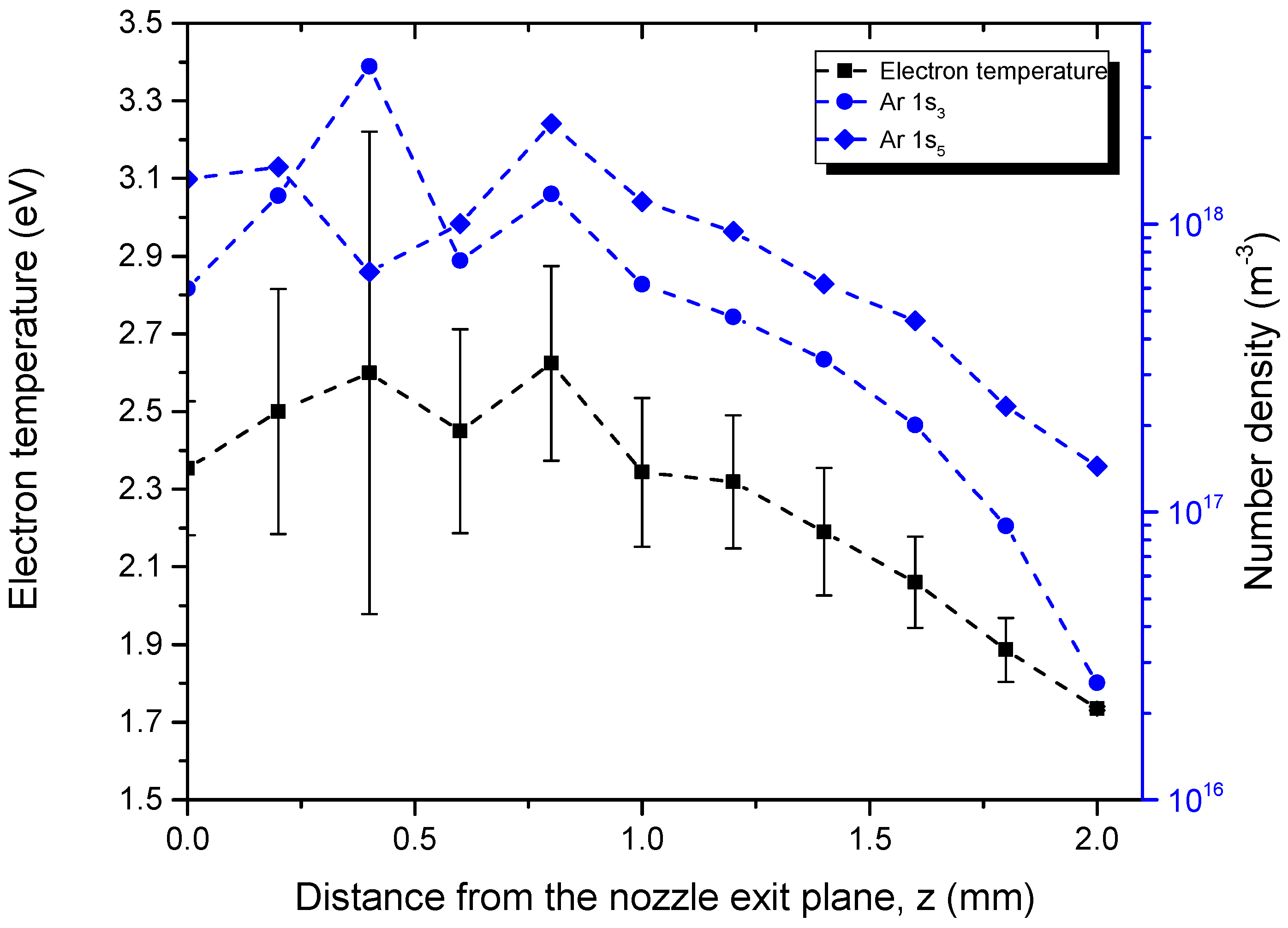
3.3. Spatially-Resolved Electron Temperature

Results for the electron temperature as found from the comparison between measured and simulated optical emission spectra from Ar $2p$-to-$1s$ transitions are presented in Figure 11. As mentioned above, $1s$ number densities obtained from OAS experiments (Figure 10) were used as inputs in the CR model. Figure 11 reveals a decay of T${}_e$ when moving away from the nozzle, starting roughly around 2.4 eV at the nozzle exit and dropping below 2 eV 2 mm downstream.

Electron temperature is an essential parameter to characterize when studying APPJs, but is nonetheless not always straightforward to estimate. The most common experimental techniques reported are the line-ratio method assuming Boltzmann equilibrium [45,46,47], the Boltzmann-plot method [46,47], the equivalent circuit model coupled with the power balance equation [48], and CR models similar to the one used in the present study [33,49,50]. As can be seen in the next lines, these multiple techniques can provide a wide range of $T_e$ values, but depending on the conditions, not all are always reliable.

Li et al. [48] estimated a constant 1.4 eV electron temperature for the entire range between 5 and 120 W, for an RF discharge in Ar at 10 L/min based on the equivalent circuit model of the discharge and by making use of the power balance equation. The equation included the power delivered and the energy losses due to radiation, ionization processes, excited states’ production, and temperature and pressure increase. The uncertainties of this technique arise from numerous sources, and the error on the electron temperature can be difficult to estimate.

Forster et al. [46] reported an excitation temperature of 1.0 eV at the exit of the tube for a discharge in Ar at 2 W at 4 L/min using a Boltzmann plot method, and the temperature went down to 0.7 eV after 2 mm. The radial study, using an Abel-inversion, showed a slightly higher electron temperature on the fringe compared to the centre of the jet, probably due to the ring shape of the jet. Using the same technique, but in a DC discharge in Ar with 2%H${}_2$, Sismanoglu et al. [47] measured an excitation temperature of 0.7 eV. This temperature was confirmed by using two Ar I lines, 603.213 and 565.070 nm, and two Cu I lines.

Finally, the modelling study of Van Gaens and Bogaerts [36] predicted T${}_e$ values around 3 eV at the exit of an argon plasma jet flowing into humid air. These values were comparable to those obtained by Hubner et al. [51] under comparable experimental conditions using temporally and spatially resolved Thomson laser scattering measurements. A summary of these results is presented in

Table 2. Comparison of the electron temperature available in the literature. The present study is reported on the last line.

Ref.	Gas	Power (W)	T${}_{\mathit{e}}$ (eV)
[36]	Ar	6.5	3.0
[46]	Ar	2	1.0 to 0.7
[48]	Ar	0–120	1.4
[47]	Ar/H${}_2$	n.a.	0.7
[51]	Ar	n.a.	3 to 0.2
[52]	Ar	4	2.2
This work	Ar	40	2.5 to 1.7

, along with the results of the present study. As can be seen, our extracted electron temperature values were somewhere in the middle of everything that could be found in the literature. As for the excited Ar level densities, the drop along the discharge axis was attributed to mixing with ambient air.

4. Conclusions

In this investigation, spectroscopic diagnostics combined with a CR model and CFD simulations were applied to an APPJ to study the Ar $1s$ level number density, as well as the electron and neutral gas temperatures along the discharge axis. OAS results revealed densities higher than ∼1 × 10${}^{18}$ m${}^{-3}$ for the metastable levels at the exit of the mini-torch nozzle. Both densities were found to decrease by two orders of magnitude over a distance of 2 mm. These results, coupled with spatially-resolved OES measurements and a collisional-radiative model, were used to estimate the evolution of T${}_e$ along the jet axis. At 40 W and 5 L/min of Ar flow, T${}_e$ at around 2.5 eV at the nozzle exit and decreased below 2 eV over 2 mm.

The neutral gas temperature measured with a thermocouple was compared to the rotational temperatures of the OH(A) and N${}_2$(C) bands fitted using the Specair software. The large difference between these species excitation temperatures, the gas temperature, and the electron temperature highlighted the non-equilibrium nature of the jet.

In future experiments, operation in different plasma-forming gases is foreseen, e.g., helium. The injection of reactive gases in the plasma afterglow through the capillary electrode, like O${}_2$ and various organosilicon precursors, will expand the possible applications of the APPJ.

References

1. Laroussi, M.; Akan, T. Arc-free atmospheric pressure cold plasma jets: A review. Plasma Process. Polym. 2007, 4, 777–788. [Google Scholar] [CrossRef]
2. Lacoste, A.; Bourdon, A.; Kuribara, K.; Urabe, K.; Stauss, S.; Terashima, K. Pure air plasma bullets propagating inside microcapillaries and in ambient air. Plasma Sources Sci. Technol. 2014, 23, 062006. [Google Scholar] [CrossRef]
3. Van Gessel, B.; Brandenburg, R.; Bruggeman, P.J. Electron properties and air mixing in radio frequency driven argon plasma jets at atmospheric pressure. Appl. Phys. Lett. 2013, 103, 064103. [Google Scholar] [CrossRef] [Green Version]
4. Sakiyama, Y.; Graves, D.B.; Jarrige, J.; Laroussi, M. Finite element analysis of ring-shaped emission profile in plasma bullet. Appl. Phys. Lett. 2010, 96, 41501. [Google Scholar] [CrossRef] [Green Version]
5. Spiekermeier, S.; Schröder, D.; Gathen, V.S.v.D.; Böke, M.; Winter, J. Helium metastable density evolution in a self-pulsing μ-APPJ. J. Phys. D Appl. Phys. 2015, 48, 35203. [Google Scholar] [CrossRef]
6. Boffard, J.B.; Jung, R.O.; Lin, C.C.; Wendt, A.E. Measurement of metastable and resonance level densities in rare-gas plasmas by optical emission spectroscopy. Plasma Sources Sci. Technol. 2009, 18, 035017. [Google Scholar] [CrossRef]
7. Benedikt, J.; Hofmann, S.; Knake, N.; Böttner, H.; Reuter, R.; von Keudell, A.; Schulz-von der Gathen, V. Phase resolved optical emission spectroscopy of coaxial microplasma jet operated with He and Ar. Eur. Phys. J. D 2010, 60, 539–546. [Google Scholar] [CrossRef]
8. Naidis, G.V. Production of active species in cold helium–air plasma jets. Plasma Sources Sci. Technol. 2014, 23, 065014. [Google Scholar] [CrossRef]
9. Walsh, J.L.; Kong, M.G. Room-temperature atmospheric argon plasma jet sustained with submicrosecond high-voltage pulses. Appl. Phys. Lett. 2007, 91, 221502. [Google Scholar] [CrossRef] [Green Version]
10. Schneider, S.; Lackmann, J.W.; Ellerweg, D.; Denis, B.; Narberhaus, F.; Bandow, J.E.; Benedikt, J. The role of VUV radiation in the inactivation of bacteria with an atmospheric pressure plasma jet. Plasma Process. Polym. 2012, 9, 561–568. [Google Scholar] [CrossRef] [Green Version]
11. Schneider, S.; Lackmann, J.W.; Narberhaus, F.; Bandow, J.E.; Denis, B.; Benedikt, J. Separation of VUV/UV photons and reactive particles in the effluent of a He/O2 atmospheric pressure plasma jet. J. Phys. Appl. Phys. 2011, 44, 379501. [Google Scholar] [CrossRef] [Green Version]
12. Nečas, D.; Čudek, V.; Vodák, J.; Ohlídal, M.; Klapetek, P.; Benedikt, J.; Rügner, K.; Zajíčková, L. Mapping of properties of thin plasma jet films using imaging spectroscopic reflectometry. Meas. Sci. Technol. 2014, 25, 115201. [Google Scholar] [CrossRef]
13. Joh, H.M.; Choi, J.Y.; Kim, S.J.; Chung, T.H.; Kang, T.H. Effect of additive oxygen gas on cellular response of lung cancer cells induced by atmospheric pressure helium plasma jet. Sci. Rep. 2014, 4, 6638. [Google Scholar] [CrossRef] [PubMed]
14. Van Rens, J.F.M.; Schoof, J.T.; Ummelen, F.C.; van Vugt, D.C.; Bruggeman, P.J.; van Veldhuizen, E.M. Induced Liquid Phase Flow by RF Ar Cold Atmospheric Pressure Plasma Jet. IEEE Trans. Plasma Sci. 2014, 42. [Google Scholar] [CrossRef] [Green Version]
15. Coulombe, S.; Léveillé, V.; Yonson, S.; Leask, R.L. Miniature atmospheric pressure glow discharge torch (APGD-t) for local biomedical applications. Pure Appl. Chem. 2006, 78, 1147–1156. [Google Scholar] [CrossRef] [Green Version]
16. Kelly, S.; Turner, M.M. Power modulation in an atmospheric pressure plasma jet. Plasma Sources Sci. Technol. 2014, 23, 065012. [Google Scholar] [CrossRef]
17. Leduc, M.; Coulombe, S.; Leask, R.L. Atmospheric Pressure Plasma Jet Deposition of Patterned Polymer Films for Cell Culture Applications. IEEE Trans. Plasma Sci. 2009, 37, 927–933. [Google Scholar] [CrossRef]
18. Walsh, J.L.; Iza, F.; Janson, N.B.; Law, V.J.; Kong, M.G. Three distinct modes in a cold atmospheric pressure plasma jet. J. Phys. D Appl. Phys. 2010, 43, 075201. [Google Scholar] [CrossRef]
19. Laroussi, M.; Lu, X. Room-temperature atmospheric pressure plasma plume for biomedical applications. Appl. Phys. Lett. 2005, 87, 28–30. [Google Scholar] [CrossRef] [Green Version]
20. Kim, J.Y.; Ballato, J.; Kim, S.O. Intense and energetic atmospheric pressure plasma jet arrays. Plasma Process. Polym. 2012, 9, 253–260. [Google Scholar] [CrossRef]
21. Léveillé, V.; Coulombe, S. Design and preliminary characterization of a miniature pulsed RF APGD torch with downstream injection of the source of reactive species. Plasma Sources Sci. Technol. 2005, 14, 467–476. [Google Scholar] [CrossRef]
22. Jarrige, J.; Laroussi, M.; Karakas, E. Formation and dynamics of plasma bullets in a non-thermal plasma jet: Influence of the high-voltage parameters on the plume characteristics. Plasma Sources Sci. Technol. 2010, 19. [Google Scholar] [CrossRef]
23. Chauvet, L.; Therese, L.; Caillier, B.; Guillot, P. Characterization of an asymmetric DBD plasma jet source at atmospheric pressure. J. Anal. At. Spectrom. 2014, 29, 2050–2057. [Google Scholar] [CrossRef]
24. Yonemori, S.; Nakagawa, Y.; Ono, R.; Oda, T. Measurement of OH density and air–helium mixture ratio in an atmospheric-pressure helium plasma jet. J. Phys. D Appl. Phys. 2012, 45, 225202. [Google Scholar] [CrossRef]
25. Knake, N.; Reuter, S.; Niemi, K.; Schulz-von der Gathen, V.; Winter, J. Absolute atomic oxygen density distributions in the effluent of a microscale atmospheric pressure plasma jet. J. Phys. D Appl. Phys. 2008, 41, 194006. [Google Scholar] [CrossRef]
26. Sarani, A.; De Geyter, N.; Nikiforov, A.Y.; Morent, R.; Leys, C.; Hubert, J.; Reniers, F. Surface modification of PTFE using an atmospheric pressure plasma jet in argon and argon+CO2. Surf. Coat. Technol. 2012, 206, 2226–2232. [Google Scholar] [CrossRef]
27. Massines, F.; Sarra-Bournet, C.; Fanelli, F.; Naudé, N.; Gherardi, N. Atmospheric Pressure Low Temperature Direct Plasma Technology: Status and Challenges for Thin Film Deposition. Plasma Process. Polym. 2012, 9, 1041–1073. [Google Scholar] [CrossRef]
28. Castaños Martínez, E.; Moisan, M. Absorption spectroscopy measurements of resonant and metastable atom densities in atmospheric-pressure discharges using a low-pressure lamp as a spectral-line source and comparison with a collisional-radiative model. Spectrochim. Acta Part B At. Spectrosc. 2010, 65, 199–209. [Google Scholar] [CrossRef]
29. Moussounda, P.S.; Ranson, P. Pressure broadening of argon lines emitted by a high-pressure microwave discharge (Surfatron). J. Phys. B At. Mol. Phys. 1987, 20, 949. [Google Scholar] [CrossRef]
30. Kramida, A.; Ralchenko, Y.; Reader, J.; NIST ASD Team. NIST Atomic Spectra Database (ver. 5.0); National Institute of Standards and Technology: Gaithersburg, MD, USA, 2012.
31. Durocher-Jean, A.; Desjardins, E.; Stafford, L. Characterization of a microwave argon plasma column at atmospheric pressure by optical emission and absorption spectroscopy coupled with collisional-radiative modelling. Phys. Plasmas 2019, 26, 1–13. [Google Scholar] [CrossRef]
32. Malyshev, M.V.; Donnelly, V.M. Trace rare gases optical emission spectroscopy: Nonintrusive method for measuring electron temperatures in low-pressure, low-temperature plasmas. Phys. Rev. E 1999, 60, 6016–6029. [Google Scholar] [CrossRef]
33. Nguyen, T.D.; Sadeghi, N. Rate coefficients for collisional population transfer between 3p54p argon levels at 300 K. Phys. Rev. A 1978, 18, 1388–1395. [Google Scholar] [CrossRef]
34. Chang, R.S.F.; Setser, D.W. Radiative lifetimes and two-body deactivation rate constants for Ar(3p5, 4p) and Ar(3p5,4p’) states. J. Chem. Phys. 1978, 69, 3885–3897. [Google Scholar] [CrossRef]
35. Zhu, X.M.; Pu, Y.K. A simple collisional–radiative model for low-temperature argon discharges with pressure ranging from 1 Pa to atmospheric pressure: Kinetics of Paschen 1s and 2p levels. J. Phys. D Appl. Phys. 2009, 43, 015204. [Google Scholar] [CrossRef]
36. Van Gaens, W.; Bogaerts, A. Corrigendum: Kinetic modelling for an atmospheric pressure argon plasma jet in humid air. J. Phys. D Appl. Phys. 2014, 47, 079502. [Google Scholar] [CrossRef]
37. Laux, C.O.; Spence, T.G.; Kruger, C.H.; Zare, R.N. Optical diagnostics of atmospheric pressure air plasmas. Plasma Sources Sci. Technol. 2003, 12, 125–138. [Google Scholar] [CrossRef]
38. Specair Software. Available online: www.specair-radiation.net (accessed on 3 October 2019).
39. Poirier, J.S.; Bérubé, P.M.; Muñoz, J.; Margot, J.; Stafford, L.; Chaker, M. On the validity of neutral gas temperature by N 2 rovibrational spectroscopy in low-pressure inductively coupled plasmas. Plasma Sources Sci. Technol. 2011, 20. [Google Scholar] [CrossRef]
40. ANSYS FLUENT 14.5, Theory Guide; ANSYS, Inc.: Canonsburg, PA, USA, 2012.
41. Launder, B.E.; Spalding, D.B. Lectures in Mathematical Models of Turbulence; Academic Press: London, UK, 1972. [Google Scholar]
42. Niermann, B.; Reuter, R.; Kuschel, T.; Benedikt, J.; Böke, M.; Winter, J. Argon metastable dynamics in a filamentary jet micro-discharge at atmospheric pressure. Plasma Sources Sci. Technol. 2012, 21, 034002. [Google Scholar] [CrossRef]
43. Niermann, B.; Böke, M.; Sadeghi, N.; Winter, J. Space resolved density measurements of argon and helium metastable atoms in radio-frequency generated He-Ar micro-plasmas. Eur. Phys. J. D 2010, 60, 489–495. [Google Scholar] [CrossRef]
44. Sands, B.L.; Leiweke, R.J.; Ganguly, B.N. Spatiotemporally resolved Ar (1s5) metastable measurements in a streamer-like He/Ar atmospheric pressure plasma jet. J. Phys. D Appl. Phys. 2010, 43, 282001. [Google Scholar] [CrossRef]
45. Zhu, X.M.; Pu, Y.K. Optical emission spectroscopy in low-temperature plasmas containing argon and nitrogen: Determination of the electron temperature and density by the line-ratio method. J. Phys. D Appl. Phys. 2010, 43, 403001. [Google Scholar] [CrossRef]
46. Förster, S.; Mohr, C.; Viöl, W. Investigations of an atmospheric pressure plasma jet by optical emission spectroscopy. Surf. Coat. Technol. 2005, 200, 827–830. [Google Scholar] [CrossRef]
47. Sismanoglu, B.N.; Amorim, J.; Souza-Corrêa, J.A.; Oliveira, C.; Gomes, M.P. Optical emission spectroscopy diagnostics of an atmospheric pressure direct current microplasma jet. Spectrochim. Acta Part B At. Spectrosc. 2009, 64, 1287–1293. [Google Scholar] [CrossRef]
48. Li, S.Z.; Lim, J.P.; Uhm, H.S. Discharge characteristics of an atmospheric-pressure capacitively coupled radio-frequency argon plasmas. Phys. Lett. Sect. A Gen. At. Solid State Phys. 2006, 360, 304–308. [Google Scholar] [CrossRef]
49. Palomares, J.M.; Iordanova, E.I.; Gamero, A.; Sola, A.; Mullen, J.J.A.M.V.D. Mixtures Studied With a Combination of Passive and Active Spectroscopic Methods. J. Phys. D Appl. Phys. 2010, 43, 395202. [Google Scholar] [CrossRef] [Green Version]
50. Iordanova, E.; Palomares, J.M.; Gamero, A.; Sola, A.; van der Mullen, J.J.A.M. A novel method to determine the electron temperature and density from the absolute intensity of line and continuum emission: Application to atmospheric microwave induced Ar plasmas. J. Phys. D Appl. Phys. 2009, 42, 155208. [Google Scholar] [CrossRef]
51. Hübner, S.; Hofmann, S.; van Veldhuizen, E.M.; Bruggeman, P.J. Electron densities and energies of a guided argon streamer in argon and air environments. Plasma Sources Sci. Technol. 2013, 22, 65011–650118. [Google Scholar] [CrossRef]
52. Farouk, T.; Farouk, B.; Gutsol, A.; Fridman, A. Atmospheric pressure radio frequency glow discharges in argon: Effects of external matching circuit parameters. Plasma Sources Sci. Technol. 2008, 17, 35015. [Google Scholar] [CrossRef]
Figure 1. Schematics of the atmospheric pressure plasma jet (APPJ) and optical emission spectroscopy (OES) setup.
Plasma 03 00005 g001
Figure 2. Emission spectrum of the Ar APPJ flowing afterglow region, 0.6 mm from the nozzle exit, integrated over 200 ms between 300 and 680 nm, and over 20 ms between 680 and 880 nm.
Plasma 03 00005 g002
Figure 3. Schematic diagram of the optical absorption spectroscopy setup.
Plasma 03 00005 g003
Figure 4. Global absorption coefficients as a function of k 0 L at the nozzle exit plane (z = 0).
Plasma 03 00005 g004
Figure 5. Radial profile of the absorption for the 751.5 nm line, 1 cm away from the nozzle exit plane.
Plasma 03 00005 g005
Figure 6. Schematic of the reactions considered in the collisional radiative (CR) model.
Plasma 03 00005 g006
Figure 7. Axial distribution of the rotational temperature of OH(A) and N 2 (C) obtained using Specair and gas temperature measured with a thermocouple, at 5 L/min of Ar and 40 W.
Plasma 03 00005 g007
Figure 8. Argon mole fraction at 5 standard litres per minute (slm) and temperature from measurement and CFD. (a) Argon mole fraction at 5 standard litres per minute (slm) and (b) temperature from measurement and CFD.
Plasma 03 00005 g008
Figure 9. Axial distribution of the measured absorption at 5 L/min and 40 W.
Plasma 03 00005 g009
Figure 10. Axial distribution of the Ar 1 s level population at 5 L/min and 40 W.
Plasma 03 00005 g010
Figure 11. Axial distribution of T e at 5 L/min and 40 W.
Plasma 03 00005 g011