Radio Frequency Oscillations in Gyrotropic Nonlinear Transmission Lines
by
Sergey Y. Karelin
, 
Vitaly B. Krasovitsky
,
Igor I. Magda
*,
Valentin S. Mukhin
and
Victor G. Sinitsin
Institute for Plasma Electronics and New Acceleration Methods, National Science Center ‘KIPT’, National Academy of Sciences, 61108 Kharkov, Ukraine
*
Author to whom correspondence should be addressed.
Plasma 2019, 2(2), 258-271; https://doi.org/10.3390/plasma2020018
Submission received: 16 January 2019
/
Revised: 3 June 2019
/
Accepted: 4 June 2019
/
Published: 8 June 2019
(This article belongs to the Special Issue High-Power Microwave and Plasma Interactions)
Abstract
:The paper considers the quasi-monochromatic radio frequency oscillations that are observable in transmission lines of doubly connected cross-sections, partially filled with a magnetized ferrite. The frequencies and amplitudes of the oscillations appearing under the impact of short carrier-free electric pulses are determined by dispersive and non-linear properties of the line’s structure. The dispersion characteristics are governed by the geometry and size of the line and the spatial arrangement in the line of the ferromagnetic material with its intrinsic dispersion. The dependences shown by the oscillation parameters in real physical experiments are reproduced and analyzed via numerical simulation within models which account separately for different physical properties of the material and the structure.
1. Introduction
The physical effects leading to direct conversion of short carrier-free electric pulses into radio frequency oscillations have been a subject of intense studies for quite a long time [1,2,3,4,5,6,7,8,9,10,11,12,13,14,15]. In fact, this possibility stands out as a real achievement in the field of high power electronics, reached over the few past decades. The early work in the field, dating back to 1960s, was centered on excitation of electromagnetic shock waves (EMSW) in transmission lines with nonlinear properties (NLTL), and formation of pulsed waveforms with a sharp leading edge [1,2]. Later on, the interest shifted toward a different, related effect, namely excitation of intense radio frequency oscillations as a result of passage of the EMSW through the NLTL. That could be observed both in lumped parameter lines containing discrete components with some kind of nonlinear behavior [3], and in waveguides filled with a ferromagnetic material [6,7,8,9,10,11,12,13,14,15]. In the first case, the possibility of varying the lumped element parameters over a wide range enabled provision of a velocity synchronism between the EMSW and the fundamental or higher-order spatial harmonic of the periodic inductance-capacitor system, i.e., vsh ≈ vph. Here vsh stands for the shock wave velocity and vph for the phase velocity of the harmonic of interest. That could cause excitation of quasi-continuous RF oscillations at the frequency of such synchronous wave. A virtually comprehensive description of the interaction between the shock and the synchronous quasi-monochromatic wave was suggested, in terms of circuit theory and 1D telegraph equations, in [2,3,4,5]. In practice, because of the relatively low allowable levels of the voltage across the L-C elements in the NLTL, the RF power never exceeded a few megawatts, and the oscillation frequencies remained at the level of hundreds of megahertz (see, e.g., [4]).
In the case of waveguide-based systems it is essential that the guide’s cross-section should topologically be an object of double connectivity, so as to admit unipolar (in a sense, DC) electric pulses to drive the system. The obviously fit candidates are coaxial waveguides and planar strip lines. Any theoretical description of such systems requires appealing to Maxwell equations with appropriate constituent relations and boundary conditions within the 3D guiding structure. The numerous real-life experiments with such NLTLs containing a magnetized ferrite core (as well as numerical simulations of the systems) have shown that a carrier-free current pulse does give rise to quasi-monochromatic oscillations [6,7,8,9,10,11,12,13,14,15], however, in contrast to the case of lumped parameter lines, the excited RF signals represent damped sinusoidal waveforms. Quite often they reveal a rather small number of quasi-periods (n = 2–10), which actually suggests a fairly large spectral line width, up to Δf/f0 ≈ 1. Meanwhile, by properly selecting geometric parameters of the NLTL and the electrical characteristics of the impulse source it proves possible to obtain output frequencies f0 about 0.3 GHz...6 GHz and pulse powers at sub-gigawatt levels [7,9,11,12].
Thus, gyromagnetic NLTLs can be seen as a new technology to produce short RF pulses of very high intensities, while being quite simple in design. Accordingly, they may prove useful for many applications with only modest demands as to spectral line purity or total radiated energy, like EMC test beds [16,17] or subsurface radar. The obvious advantage of such systems is their ability to operate without employing intense particle beams and high vacuum. Recently, a series of operable installations were presented by teams from Russia, the UK, USA, and Ukraine [7,8,9,10] that demonstrated possibilities for extracting the RF oscillations from the limited volume of the transmission line and radiating it into free space.
Still, despite these practical achievements and continued efforts of many researchers, the underlying physics remains poorly understood. The widely shared idea concerning reasons for the appearance of the oscillations has been the impact of the precession experienced by the magnetization vector in the ferromagnet about the direction of the total DC magnetic field in the material [6,8,13,15]. Meanwhile, this effect alone cannot explain many of the features shown by the oscillatory signal, nor its dependences upon parameters of the transmission line and its filling material, including the oscillation frequency itself. This paper is an attempt at summarizing the better established facts on the generation of RF oscillations in NLTLs and suggesting a consistent electrodynamic vision of the principal effects.
2. Wave Processes in the NLTL
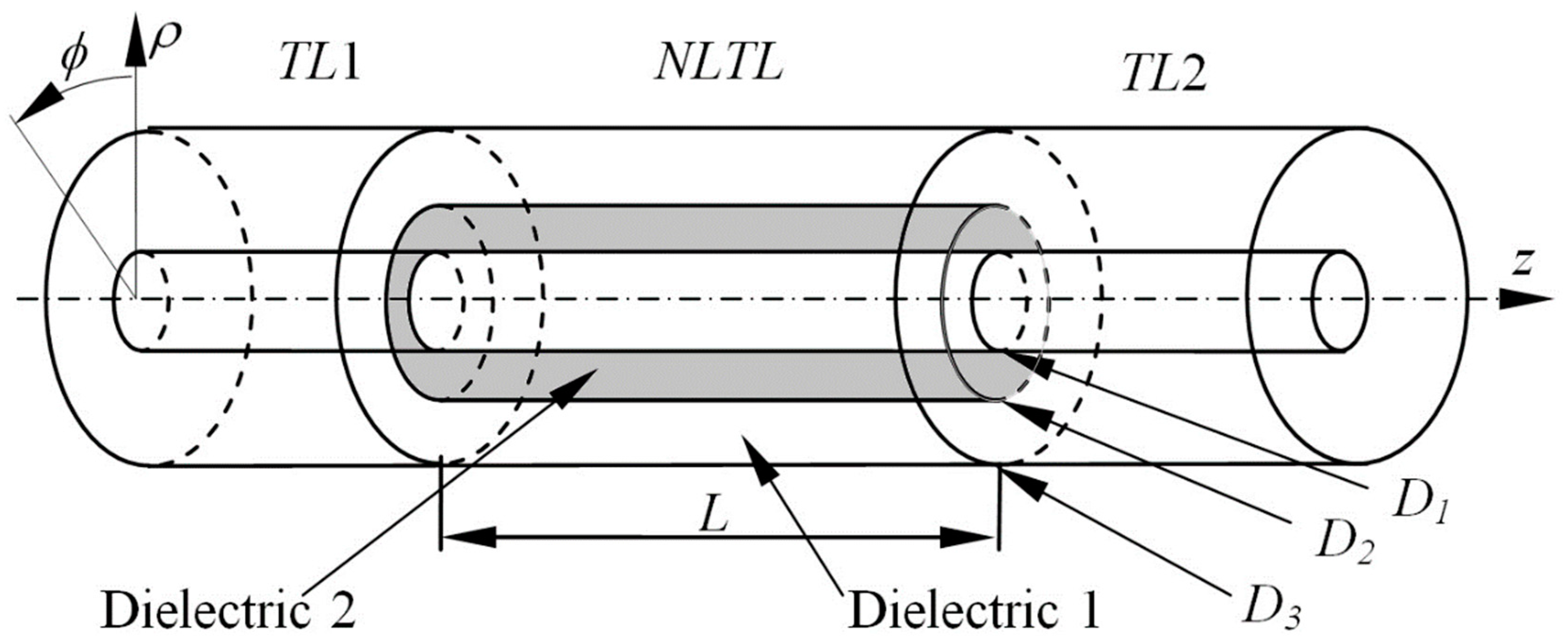
The coaxial structure used in our (and other) experiments (Figure 1) will be described in a cylindrical frame of reference (z, ρ, φ), where z is the coordinate along the line’s axis; ρ the radial, and φ the angular coordinate. It involves two uniform lines, TL1 and TL2, at the input and output, respectively, and the line NLTL that is partially filled with a ferrite. In recent studies by the present writers [10,11,12] the cross-section sizes of all three TLs were the same, D3 = 52 mm and D1 = 20 mm, which figures determined a 38 Ohm impedance for the TEM mode, and the lengths were 1000 mm for TL1 and TL2, and 800 mm for the NLTL. The TL1 and TL2 lines were fully filled with an isotropic dielectric with constant parameters (e.g., permeabilities ε = 2.25 and μ = 1, like in [10]), whereas in the NLTL the filling medium occupied two layers. The outer one, D2/2 ≤ ρ ≤ D3/2, contained the same dielectric as TL1, while the space D1/2 ≤ ρ ≤ D2/2 accommodated a cylindrical ferromagnetic core with D2 = 32 mm (actually, a set of closely spaced ferrite beads). The entire structure was placed in a DC magnetic field H0 = ezH0 provided by an external solenoid. The geometric and electrical parameters of the similar structures employed by other workers, such as line diameters D, lengths L, magnitudes of ε and μ, and the pre-magnetizing (bias) field H0 [6,7,8,9,15], were rather different. So, to compare and interpret the reported results it may prove expedient to suggest some scaling parameter, introducing an effective uniformity of the electromagnetic conditions. A variant of using such scaling parameter, k, is described in Section 3.2 below. It assumes a proportional variation of the waveguide’s transverse dimensions D′i = Di/k, and the pulsed voltage at the line’s input, U′ = U/k.
2.1. Wave Modes
The processes taking place in the system can be outlined as follows. The unipolar voltage surge fed into TL1 from an external pulse-forming source travels toward the front edge of the NLTL. The angular uniformity of the geometry suggests periodicity of the field distributions throughout, such that field magnitudes registered at φ = φ0 + 2π shall be equal to the relevant values at φ = φ0, and hence the angular dependences of the wave fields be exp(inφ) with n = 0, ±1, ±2, etc. In spectral terms, the wave fields represent infinite sets of harmonic components, ΣCnRn(ρ)expi(nφ+ωt-κz)dω, where κ is the propagation constant and Cn and Rn are, respectively, the amplitude and the radial distribution function in the n-th component of a specific field vector, at a frequency ω. The incoming frequency spectrum extends from ‘almost DC’ to 1/tr, where tr is the pulse’s rise time. The highest frequency in the set determines the ‘sharpness’ of the pulsed waveform edge. The lowest, of amplitude C0 about U0/(D3−D1) carries the major part of the pulse’s energy (U0 is the peak voltage amplitude of the pulsed waveform). Since the input line, TL1, involves no structural non-uniformity or anisotropy, the ‘DC’ pulse may travel through it in the form of a ‘dispersionless’ (TEM) mode where its participating spatial components are, by virtue of excitation, only two, namely the radial electric, Eρ (associated with the voltage across the line conductors) and the azimuthal magnetic Bφ = Hφ, proportionate to the current through the line. The TEM mode is characterized by the angular uniformity ∂/∂φ = in = 0, such that all frequencies travel at the same speed. Accordingly, the term ‘dispersionless’ just means that all frequency components obey the same linear dispersion law ω = κv. Upon entering the ferrite-filled part of the line the signal can no more exist as a wave packet wherein all frequency components belong to a spatial mode with the same dispersion law ω = ω(κ). First, because any wave mode with non-zero Eρ and Bφ gets diffracted at the dielectric-ferrite interface (where the electric and the magnetic parameters of the medium change abruptly), and hence acquires longitudinal components, Ez and Bz, which the initial Eρ and Bφ are coupled to through the Maxwell equations, e.g.,
Here, the magnetic inductance is B = μ0 (H+M), with M being the magnetization vector and μ0 the permeability of free space. As concerns electromagnetic excitations, the n = 0 (TEM) mode is not the only solution that can be excited here. The modes with │n│ ≥ 1 may involve more (up to all six) spatial field components, posing as hybrid EH or HE modes, and possess different, often intricate dispersion laws. The n = 0 mode itself transforms into a TM mode with three spatial components, Eρ, Bφ, and Ez, and reveals a slightly nonlinear dispersion law [18]. (For this reason, it is sometimes called the ‘quasi-TEM’ mode). The full set of wave modes supported by the transmission line is determined by its dispersion properties which are dictated by the line’s geometry and size and the type of constituent relations for the filling material. The dynamics of variations in M can be described with the phenomenological Landau–Lifschitz (L-L) equation, e.g., taken in Gilbert’s form [19]
which just provides the constituent relation B = B(H). Here γ = 2.8 × 10¹⁰ Hz/T is the gyromagnetic ratio and H denotes the total magnetic field in the medium. The magnetic field H in Equation (1) is to be estimated from the Maxwell equations, with due account of all boundary conditions for the E and B fields, so as to ‘automatically’ involve the so called de-magnetizing terms owing to finite sizes of the ferrite beads and the core as a whole [19]. Next, α < 1 is a phenomenological parameter of this macroscopic equation, accounting for magnetic relaxation effects.
∂M/dt = −γμ0[M × H] − (γαμ0/Ms)[M × [M × H]],
Considering the pulse propagation through the line we assume that the ferromagnetic core was initially magnetized by the DC field H0 almost to the saturation level M0 = ezMs. Now it is re-magnetized under the impact of the perpendicular field eφHφ which is produced by the z-oriented pulsed current. That field may be represented as Hφ = H0φ + hφ(t), where H0φ is a ‘nearly DC’ component of the incoming pulse, of a frequency about 1/τ with τ being the total pulse duration, such that H = ezH0 + eφH0φ + h(t). Accordingly, the magnetization vector M acquires spatial components oriented along the ρ-, φ-, and z-directions, both static and varying with non-zero frequencies. The variations of Mρ and Mφ with time represent the precession motion of M around the direction of the total magnetic field H.
As can be seen from Equation (1), the B = B(H) relation is (a) nonlinear and (b) anisotropic. Qualitatively, the effects of magnetic nonlinearity can be described in two ways:
1. By introducing an ‘effective magnetic permeability’ of the ferrite along the z-axis, which would be dependent on the magnetic field strength, for example like μ = 1 + M(H)/H. Within this approach, the propagation velocity v = c(εμ)−1/2 of the pulsed wave is treated as dependent on the amplitude of Hφ (i.e., current amplitude). As a result, the higher-amplitude pulse components run in advance of the lower-amplitude ones, thus sharpening the front edge and provoking shock formation. Of course, this is a rather simplified treatment, as the M = M(H) and, hence B = B(H) are not scalar relations. The refractive index c/v can hardly be associated with any scalar ‘effective μ’.
2. By considering the pulse propagation as a process of spectrum transformation and mode conversion along the line. Then the Maxwell set and the L-L-G Equation (1) need to be brought to the frequency-domain representation,
where δ(ω − ω′), etc., is Dirac’s delta. The coupling of the magnetization vector’s frequency components owing to nonlinearity becomes explicitly evident. Accordingly, the formerly independent eigenmodes specified by the linear-approximation solutions for the E and B fields get coupled, too. A linear in h solution to Equation (3) yields the familiar magnetic permeability tensor μ [19]. With regard to pulse propagation, a major effect of nonlinearity is generation of higher-order harmonics by each component from the continuous spectrum presented by the pulse. As long as they all travel, within the TEM mode, at nearly equal phase velocities (close to the pulse’s group velocity vg), we observe sharpening of the pulse’s edge. When some of the higher frequency components gets close to and beyond the cut-off frequency, fcr, for a dispersive TM, TE or a hybrid mode potentially supported by the line, that wave mode may be excited and then run downstream the line at its phase velocity vph. If the excited mode were faster than the shock wave (vph > vsh), it would be seen as a decaying sine waveform. The rate of decay might be reduced or even replaced by amplification, should the wave happen to be in a velocity synchronism with its coupled partner. That is another important effect owing to nonlinearity.
iωM(ω) = −γμ0∫dω′dω″[M(ω′) × H(ω″)] δ(ω − ω′ − ω″) −
(γαμ0/Ms)∫dω′dω″dω′″[M(ω′) × [M(ω″) × H(ω′″)]]δ(ω − ω′ − ω″ − ω′″),
(γαμ0/Ms)∫dω′dω″dω′″[M(ω′) × [M(ω″) × H(ω′″)]]δ(ω − ω′ − ω″ − ω′″),
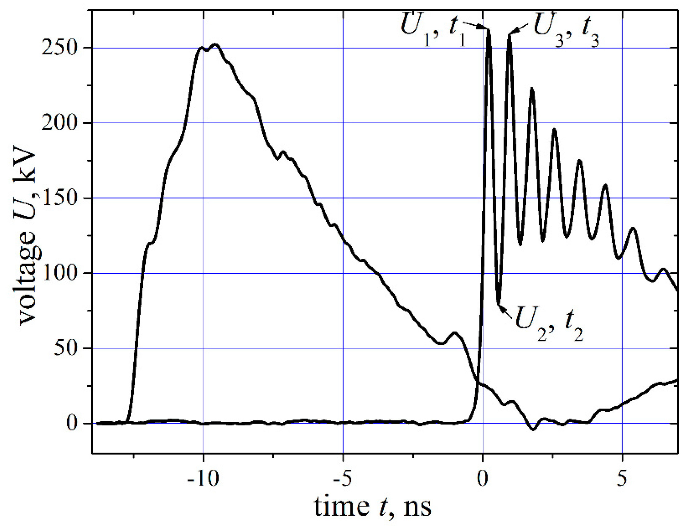
The linear in h(ω) solution to the L-L-G+Maxwell equation set representing the magnetic wave in the ferrite also looks like a decaying sine wave, which has led many writers (e.g., [6,8,9,13,15,20]) to believe that the arising oscillations are associated exclusively with precession of the magnetization vector. However, the latter is often estimated for a boundless specimen of the ferromagnetic material, without account of demagnetization effects [13,20]. Meanwhile, the frequency of magnetic moment precession is not the only characteristic frequency in the structure. The NLTL, as a line of finite-sized cross-section (and containing a layered insert at that) may support linear-approximation modes obeying a variety of dispersion laws that may involve cut-off frequencies, unlike the TEM mode. The electromagnetic eigenmode frequencies are given by a secular equation following from the full set of Maxwell equations, with proper boundary conditions and constituent relations, rather than the equation of motion for the M-vector alone. The cut-off frequencies are determined by transverse dimensions of the guiding structure. The description of the precession motion of M involves magnitudes like ω0 = μ0γH0, ωM = μ0γMs, and ωφ = μ0γH0φ. In a number of experiments (e.g., [6,8,13,15]), the corresponding frequencies f0, fM, etc., lay below 1 GHz (with H0 ranging from about 10 kA/m to 30 kA/m), while the recorded oscillation frequencies were between 0.3 GHz and 6 GHz. In fact, the magnitudes ω0, ωM etc, each having the dimension of frequency, appear in the form of combinations ω0 + ωM, (ω2 − ω02), etc., in frequency-domain solutions for components of the magnetic permeability tensor (see [19]) that determine variations in the magnetization vector M. Note that in every specific experiment H0 stayed constant, whereas Hφ changed noticeably over the duration of the current pulse. A series of experiments and simulations [11,12,14] performed with ‘triangular’ pulse waveforms (see below, Figure 2) are, in this respect, of special interest. Throughout the extended trailing edge, the magnitude of Hφ changes by a factor greater than 10, while the RF oscillation frequency never varies by more than 15%...25%. This small amount of frequency variations, compared with the greatly changing pulse amplitude, apparently suggests a rather low significance, under the conditions of a specific experiment, of the magnetic state of the medium, i.e., of magnetization dynamics. Then we have to admit that the oscillation frequency is not (at least, not always is) related as tightly to the M-vector precession.
2.2. Size Dependences
As an alternative, consider the dependences upon sizes of the structural elements. The great many experiments with nonlinear TLs, showing a variety of outer diameters D3, sizes of the ferrite beads, and magnitudes of the magnetic fields, allow bringing their results on the oscillation frequency f to the general form f~D−1. Thus, Dolan [6] operated with coaxial lines of very small diameters (D3 ≈ 3 mm) and observed oscillations at a high frequency f ≈ 6 GHz. A series of real-life experiments [7,8,9] and numerical simulations [12] performed with a variety of NLTL diameters revealed good agreement between the frequency vs. size relation and the formula f~D−1. With the diameters D3 varying from 20mm to 50 mm the oscillation frequencies changed between 2.3 GHz and 0.9 GHz. Gubanov et al. [7] experimented with lines of a large diameter ~80 mm and observed oscillations at lower frequencies (0.8 GHz…2 GHz). Finally, the writers [15] employed TLs of a still larger diameter (275 mm) and obtained a much lower frequency, f~0.3 GHz. The relationship between the oscillation parameters and transverse dimensions of the NLTL is shown in Figure 3 as dependences of the oscillation frequency and relative amplitude, A = (U1 − U2)/(U1 + U2), upon the scaling factor k. This latter assumes a proportional variation of the waveguide’s transverse dimensions D′i = Di/k, and the pulsed voltage at its input, U′ = U/k. With this proportion held, the current-induced azimuthal magnetic field Hφ re-magnetizing the ferrite remains unchanged. The k = 1 magnitude of the scaling factor relates to the case D3/D2/D1 = 52 mm/32 mm/20 mm. The results of simulations, also presented in Figure 3, confirm the trend revealed in the experiment, namely that with an increase of the transverse dimensions, the oscillation frequency decreases, whereas their amplitude increases. Details of the computational work, in a version of the FDTD, were earlier described in [14]. Additionally, it can be seen that with smaller transverse dimensions (smaller k) the oscillation frequency reaches a certain high level where it almost stops changing further. Thus, both experiments and numerical calculations indicate that the oscillation frequency is, more often than not, related to transverse dimensions of the coaxial NLTL, while its relation to magnetization parameters (the bias field in particular) is not straightforward.
3. Numerical Modeling
The excitation of RF oscillations in a coaxial ferrite-filled NLTL by a current pulse was analyzed by the present authors [10,12,14] with the help of a time-domain technique based on direct numerical integration of the Maxwell equation set, together with the Landau–Lifschitz equation of state for the ferromagnetic medium [19]. The computations were done in a version of the FDTD method [14], which for the time being is still limited by the assumption of n = 0 (a 2D + code involving z and ρ coordinates). The dielectric permittivities of the insulating dielectric and the ferrite were, respectively, ε1 = 2.25 and ε2 = 16, and also ε1 = 80 and ε2 = 16 in the last of the simulations. The ratio of diameters was D2/D1 = 1.6. The saturation level Ms of the magnetic moment and the relaxation coefficient α in the L-L-G equation were assumed as 300 kA/m and 0.1, respectively.
Figure 4 presents the frequency and relative amplitude of the oscillations calculated as functions of the ferrite outer diameter D2 (for a fixed geometry of the line, D3/D1 = 52 mm/20 mm). With an increase in the filling ratio of the NLTL with the ferromagnetic material the f = f(D2) dependence demonstrates a tendency toward reaching a certain low level, admittedly near the lowest cut-off fcr min. This behavior can be interpreted as an increase in the ‘effective’ ε and μ, hence a gradual decrease of (εμ)−1/2. The relative oscillation amplitude, A, presented as a function of the ferrite diameter (i.e., line’s filling ratio, see Figure 4) demonstrates a maximum at D2/D3 = 40%…50%.
The above presented results are in agreement with the calculated dependences of the oscillation frequency versus the outer diameter, f = f(D3). Figure 5 demonstrates a monotonic decrease in f with increasing D3, and its tendency toward a steady value. Actually, this reflects the physically meaningful dependence on the difference of the radii, 0.5(D3 − D2) that determines the critical frequencies fcr for TM0m modes. If the external diameter D3 is reduced, approaching the ferrite outer diameter D2, then at D3 = D2 we get a line completely filled with the ferrite. The line with these new parameters (a smaller D3 and a filling ratio of one) expectedly demonstrates a higher oscillation frequency (Figure 5). These data point to the decisive role of the structural non-uniformity within the waveguide’s cross-section in controlling the electromagnetic wave motions.
To analyze the impact of individual mechanisms responsible for dispersion, a few targeted numerical experiments were conducted, concerning excitation and conversion of modes in a coaxial waveguide partially filled with a magneto-sensitive medium. The transformations of the initial carrier-free pulse in the three-sectional coax line were simulated numerically within three models of the middle section, designated as the NLTL. The differences in the models concern the internal layer D1/2 ≤ ρ ≤ D2/2 which represents the magnetic-sensitive material. The cases analyzed were as follows,
(i) Both the ε and μ of the magnetic material were taken to be constant scalar magnitudes, however different from the parameters of the outer layer, D2/2 ≤ ρ ≤ D3/2.
(ii) The dielectric permittivity ε was a scalar constant value, while the permeability μ a scalar dependent on H (‘uniaxial’, nonlinear magnetic).
(iii) The layer represented a gyrotropic, magnetically nonlinear medium (ferromagnet) with a constant isotropic dielectric permittivity.
With this choice of materials we considered three electrodynamic models of the entire transmission line, namely:
model I, an electromagnetically linear one;
model II, accounting for nonlinear effects, and
model III, a nonlinear and anisotropic model incorporating the L-L Equation (1).
3.1. Linear Model, I
Within the linear model the material parameters of both dielectric layers in the middle section were constant but unequal values. Once again, the outer dielectric possessed μ1 = 1 and ε1 = 2.25 as in TL1, whereas the internal dielectric was characterized by μ2 = 7 and ε2 = 16. The Landau–Lifschitz equation was not included in the computations, so the constituent relation was B = μ0μ2H. The input line TL1 was fed with short ‘triangular’ pulses of a 10 ns duration, having sharp leading edges 0.2 ns…3 ns in width. The simulations showed that pulses with a relatively wide front edge (rise times greater than 1.5 ns) traveled through the line without visible distortions. Contrary to that, a pulse with an initially shorter rise time became a different waveform at the output. Its leading edge spread wider and oscillations of a gradually decreasing amplitude appeared, overlaid on the top (see Figure 6a).
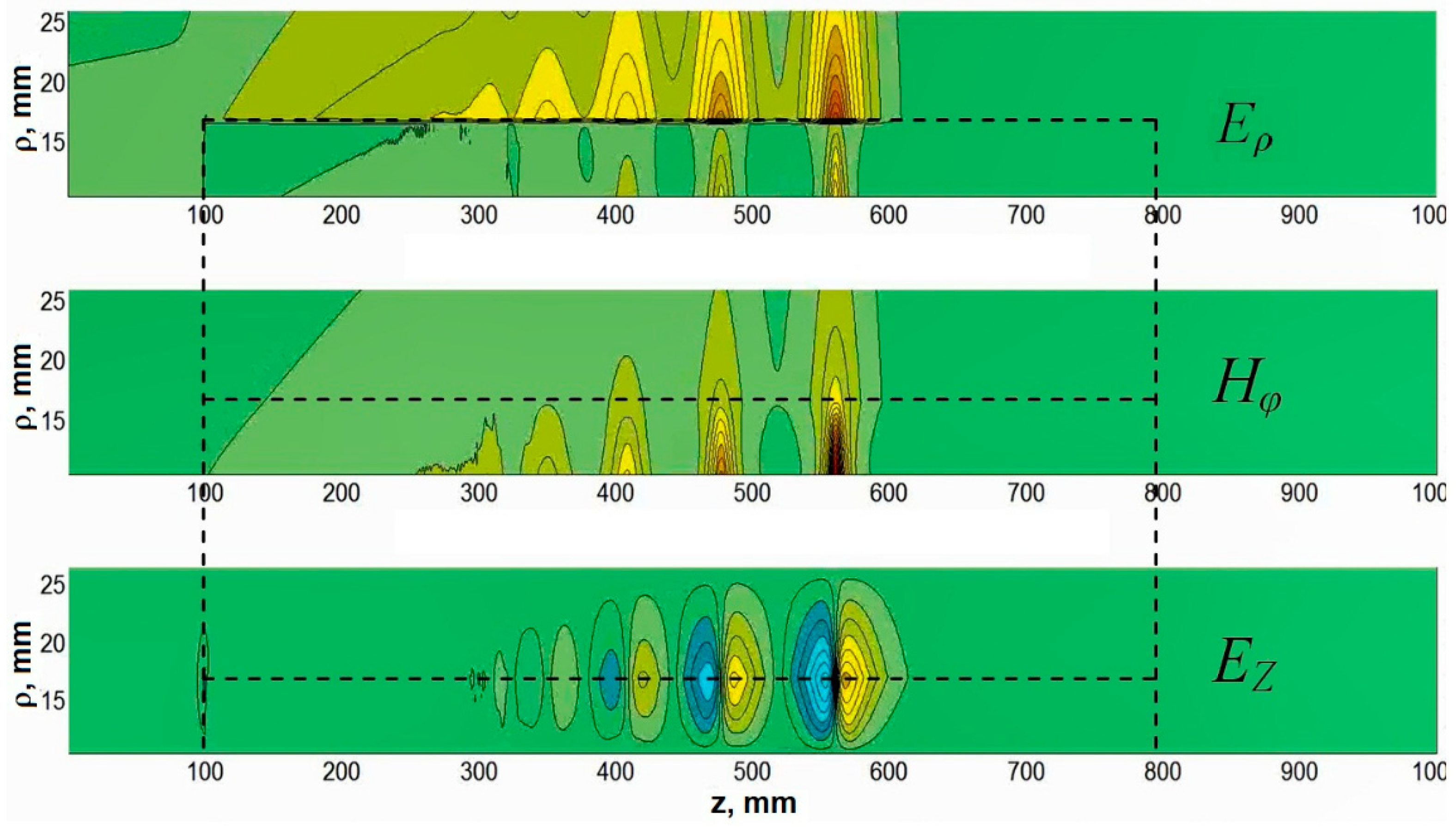
Shown in Figure 7 are 2D dynamics of the Eρ, Hφ, and EZ field components in a ‘triangular’ pulsed electromagnetic wave with parameters U0 = 200 kV, half-height pulse length τp0.5 = 5 ns, and pulse rise time tr = 0.8 ns. As discussed above, all frequency components of the wideband pulsed signal traveled through TL1 in the form of a TEM mode and got scattered at the entrance to the middle part of the line. Some of them transformed into a dispersive ‘quasi-TEM’ mode, having acquired a longitudinally oriented electric component, Ez. Others, whose frequencies happened to be close to cut-off frequencies of some higher-order TM or TE modes could give rise to these—provided that, in addition to the frequency proximity, there also were matching of propagation constants and field vector orientations (polarization). Note that such wave modes (clearly identifiable as TM0p) can be seen in Figure 7 where they follow behind the main pulse’s body as their phase velocities are lower than the speed of the ‘quasi-TEM’ packet.
3.2. Nonlinear Scalar Model, II
Consider the case where the dielectric constants of both filling materials in the TL are constant values and the medium in the internal layer shows nonlinear magnetic properties. Assuming it to remain isotropic (to emphasize the effects owing to nonlinearity) we write B = μ0μ2(H)H, taking the scalar magnetic permeability to be of form
which can be derived from the solution of Equation (2) for the magnetization vector. Let the saturated magnetization be Ms = 300 kA/m, which we figure to be representative of a lot of ferrite grades. The bias field corresponding to the point of saturation on the ‘technical magnetization‘ curve will be taken as H0 = 30 kA/m. The computations show the quasi-periodic oscillations to appear even with a sizable initial width of the incoming pulse (see Figure 6b), unlike the linear case. The rise time tr of the pulsed wave is reduced in the course of its propagation through the NLTL, i.e., the spectrum is enriched in higher frequency components, due to non-linearity, at the expense of low frequencies. This effect of pulse sharpening may become stabilized because of dispersion, in particular near the cut-off frequency of some higher-order mode which would manifest itself as an oscillatory waveform. In the present numerical experiment, the width of the pulse’s leading edge was stabilized at tr ≈ 0.4 ns, as measured at the output. At this point, it is worth comparing the oscillation amplitudes at different positions along the line length, as presented in Figure 6a,b, for the linear and nonlinear models, respectively. In the linear case, the peak amplitude remains nearly unchanged as the pulse travels along the line (see curves 2–4 in Figure 6a). In the non-linear case (Figure 6b) the homologous waveform crests in curves 2–4 grow in magnitude as the pulse travels from position 2 to position 4. This means that the principal energy carrying mode of the NLTL has become coupled to and started pumping energy into the dispersive mode(s) posing as oscillations. The evolution of the Eρ, Hφ and EZ field components can be seen in Figure 8.
3.3. Nonlinear Gyrotropic Model, III
The ‘full’ nonlinear and gyrotropic model III suggested application of the Landau–Lifschitz equation as a constituent relation for the Maxwell set. Similar as with model II, the saturated magnetization was Ms = 300 kA/m. The relaxation parameter α in Equation (2) was taken as α = 0.1. The results obtained in the numerical experiment with H0 = 30 kA/m; U0 = 200 kV; τp0.5 = 5 ns, and tr = 2 ns (an initially broad leading edge) are given in Figure 9. Once again, the pulse voltages estimated at several locations within the NLTL reveal a noticeable growth in amplitude, admittedly as a result of interaction between the now coupled eigenmodes of the linear approximation. In addition, the oscillation period seems shorter than in the case of model II. In our view, this may be evidence for involvement of a different, higher-order waveguide mode matched with a small number of frequency components from the ‘quasi-TEM’ wave packet. The ‘quasi-TEM’ mode is noticeably dispersive at higher frequencies, hence frequency-selective as for getting in speed synchronism with other modes.
Note the fair agreement between experimental results on RF frequencies and amplitudes reported in [10,11] and the numerical estimates of Model III. The discrepancy remains within 20%. Similar as the findings of [10,11], the computed results offer a preferred length about 500 mm for the ferrite core, with which the output amplitude of the RF wave is the highest. With fixed initial parameters of the driving pulse, a further increase in the length of the nonlinear line did not lead to higher output amplitudes, admittedly because of losses of the RF power in the ferrite (curve 4 in Figure 9).
Upon comparing Figure 8 and Figure 10 it becomes evident that dispersive effects are stronger in the case of a gyrotropic nonlinear medium, compared with the isotropic nonlinear material of model II. The result is a noticeable increase in the full extent of the passing pulsed signal.
The above discussed models have permitted analyzing different aspects of RF excitation in non-uniformly filled coaxial transmission lines. The properties of the filling material have been shown to substantially influence parameters of the RF signal at the output, such as amplitude, median frequency and spectral width. At the same time, the characteristic temporal behavior of the oscillatory process, namely appearance of only a limited number of quasi-periods of diminishing magnitude, persisted in a majority of cases. This is evidence for an impact nature of wave excitation. When a RF pulse travels down the line with a linear response function (model I), it is only natural that it remains a decaying waveform. In the structures with nonlinearity (model II and model III) one might expect a lower rate of attenuation, or even an increase in the amplitude of the oscillatory signal, owing to nonlinear coupling of the formerly independent wave modes. The coupling may result in energy transfer from one mode to another, subject to the conditions of frequency and wavenumber matching or, in other words, velocity synchronism. As can be seen from model III, the speed shown by the shock wave (i.e., the group velocity of a set of quasi-TEM modes) is vsh = (0.12…0.14)c under the conditions assumed for the model. Meanwhile, the phase velocity of the arising dispersive mode (admittedly, TM01) can be estimated as 0.7c, since it is concentrated mostly out of the ferrite, in the isotropic dielectric with a modest ε1 = 2.25. The result is the decaying sine waveform once again. Meanwhile, the high degree of speed synchronism between the shock wave and its concurrent mode that was reported in [4,5] for lumped parameter lines with feedback, allowed obtaining radio pulses of greater length and virtually constant amplitude. The goal of generating (quasi)monochromatic propagational radio pulses of extended length in actual 3D coaxial transmission lines can be reached through creating there similar synchronism conditions, vph = vsh.
3.4. Nonlinear Gyrotropic Model, IV
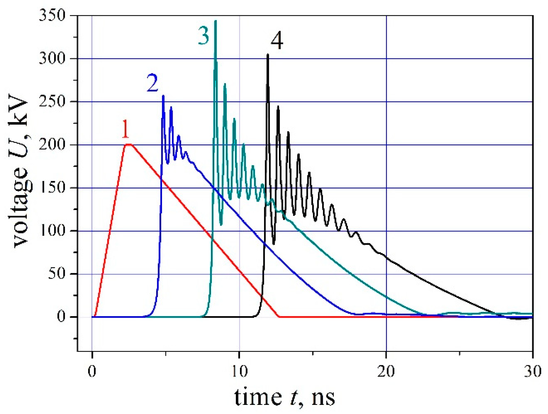
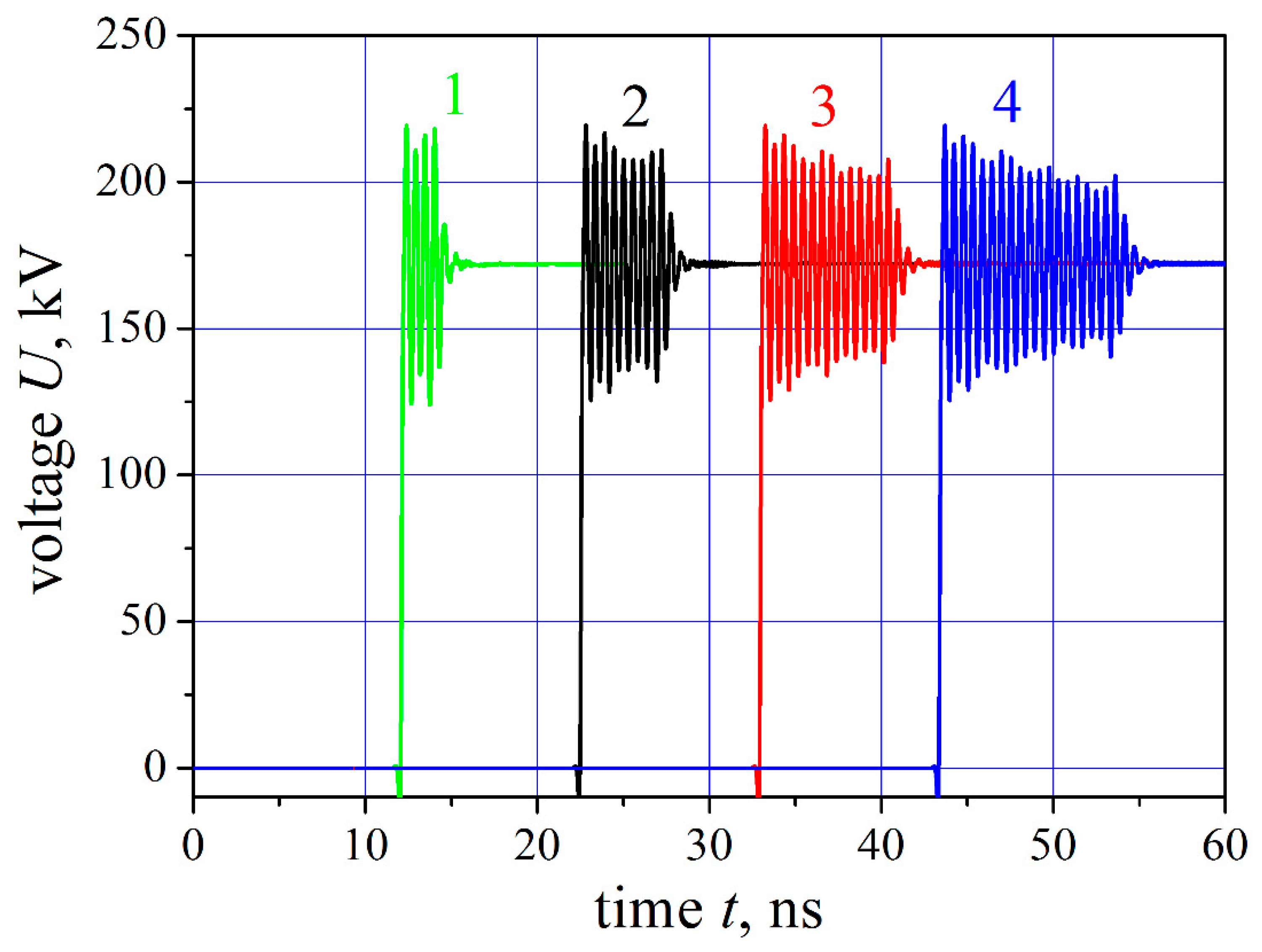
To analyze the possibility of providing a speed synchronism between the main body of the shock and the emerging waveguide mode, yet another numerical experiment was performed. Now, the outer dielectric 1 was represented by a material with a much higher dielectric constant, ε1 = 80 (and μ1 = 1). The phase velocity of the TM01 can be evaluated as vph01 ≈ 0.11c, which value is close to the velocity of the shock wave traveling through the ferrite. The anticipated sinusoidal wave and the shock wave, while being localized in different sub-spaces of the waveguide, happen to be synchronized in velocity, like in [5]. The results of this simulation are presented in Figure 11. The input port of the structure (the isotropic line TL1) was fed with a ‘step function’ voltage pulse of front-edge duration 1.5 ns and a 200 kV. The radio pulses at the output were characterized by a short front edge (~120 ps), followed by chains of practically monochromatic oscillations of amplitudes about 50 kV and central frequency 1.79 GHz. The number of RF periods in a chain was proportional to the ‘active’ length of the NLTL, with nearly constant values for the central frequency and amplitude. Accordingly, the frequency spectrum at the output demonstrates a distinct peak at 1.79 GHz with a 190 MHz width at the half-height level.
4. Conclusions
The propagation of a short current pulse through a coaxial transmission line that involves a section partially filled with a ferromagnetic material has been analyzed numerically to clarify the role of different physical effects in converting the ‘DC’ pulse into quasi-monochromatic radio frequency oscillations. The results obtained are in agreement with the concept of a synchronous wave, emphasizing the role of speed synchronism between the main body of the traveling shock wave and a waveguide-type mode. The latter appears and may stay supported in the coaxial line owing to the interplay of dispersive and nonlinear effects in the structure involving a gyrotropic medium. The analysis was performed within four particular models which allowed treating separately the basic effects potentially responsible for the appearance of the oscillations and their amplification and/or decay along the line. Contrary to the widely shared concept, the central frequency of the wideband oscillations is not always associated with the magnetic moment’s precession in a ferrite close to saturation. Depending on the total diameter of the coaxial waveguide, size of the ferrite core, spatial nonuniformity of the filling, and its electric and magnetic parameters, the oscillations may be represented by various eigenmodes in the line with their specific frequencies and dispersion laws.
Author Contributions
V.B.K. and V.S.M. designed and fulfilled the experiments; S.Y.K. performed computations and analysis of the experimental data; I.I.M. and V.G.S. analyzed the data, suggested theoretical interpretations and wrote the paper.
Funding
This research received no external funding.
Conflicts of Interest
The authors declare no conflict of interest.
References
- Belyantsev, A.M.; Bogatyryov, Y.K.; Solovyova, L.I. Producing electromagnetic shock waves in transmission lines containing non-saturated ferrite material (in Russian). Izv. VUZ Radiofiz. 1963, 6, 561–571. [Google Scholar]
- Freidman, G.I. The structure of electromagnetic shock waves in two-conductor transmission lines in dependence on linear-approximation dispersion properties of the lines. Izv. VUZ Radiofiz. 1963, 6, 536–550. (In Russian) [Google Scholar]
- Belyantsev, A.M.; Kozyrev, A.B. Local dispersion effects in transient processes during high frequency generation by an electromagnetic shock. (Sov.) J. Technol. Phys. 1998, 68, 89–95. (In Russian) [Google Scholar]
- Belyantsev, A.M.; Dubnev, A.I.; Klimin, A.I.; Kobelev, Y.A.; Ostrovski, L.A. Radio frequency pulse generation by an electromagnetic shock wave in a ferrite-filled transmission line. (Sov.) J. Technol. Phys. 1995, 65, 132–142. (In Russian) [Google Scholar]
- Belyantsev, A.M.; Kozyrev, A.B. Generation of high-frequency oscillations by the front edge of an electromagnetic shock in coupled transmission lines showing anomalous and normal dispersion. (Sov.) J. Technol. Phys. 2001, 71, 79–82. (In Russian) [Google Scholar]
- Dolan, J.E. Simulation of shock waves in ferrite-loaded coaxial transmission lines with axial bias. J. Phys. D Appl. Phys. 1999, 32, 1826–1831. [Google Scholar] [CrossRef]
- Gubanov, V.P.; Gunin, A.V.; Kovalchuk, O.B.; Kutenkov, V.O.; Romanchenko, I.V.; Rostov, V.V. Efficient transformation of high voltage pulsed energy into high frequency oscillations as performed in a transmission line with a saturated ferrite. J. Technol. Phys. Lett. 2009, 35, 81–87. [Google Scholar]
- Reale, D.V. Coaxial Ferromagnetic Based Gyromagnetic Nonlinear Transmission Lines as Compact High Power Microwave Sources. Ph.D. Thesis, Texas Tech University, Lubbock, TX, USA, December 2013. [Google Scholar]
- Rostov, V.V.; Bykov, N.M.; Bykov, D.N.; Klimov, A.I.; Kovalchuk, O.B.; Romanchenko, I.V. Generation of subgigawatt RF pulses in nonlinear transmission lines. IEEE Trans. Plasma Sci. 2010, 38, 2681–2687. [Google Scholar] [CrossRef]
- Karelin, S.Y.; Magda, I.I.; Mukhin, V.S. A test bed for EMC analyses with ultra-short pulses of complex spectral content. Probl. At. Sci. Technol. 2017, 112, 47–51. (In Russian) [Google Scholar]
- Gadetsky, N.P.; Karelin, S.Y.; Magda, I.I.; Shapoval, I.M.; Soshenko, V.A. Impact of ultra-short wave pulses on the PC. Probl. At. Sci. Technol. 2017, 112, 52–57. (In Russian) [Google Scholar]
- Ahn, J.-W.; Karelin, S.Y.; Kwon, H.-O.; Magda, I.I.; Sinitsin, V.G. Exciting high frequency oscillations in a coaxial transmission line with a magnetized ferrite. Korean J. Magn. 2015, 20, 460–465. [Google Scholar] [CrossRef]
- Ahn, J.-W.; Karelin, S.Y.; Krasovitsky, V.B.; Kwon, H.-O.; Magda, I.I.; Mukhin, V.S.; Melezhik, O.G.; Sinitsin, V.G. Wideband RF radiation from a nonlinear transmission line with a pre-magnetized ferromagnetic core. Korean J. Magn. 2016, 21, 450–459. [Google Scholar] [CrossRef]
- Karelin, S.Y.; Krasovitsky, V.B.; Magda, I.I.; Mukhin, V.S.; Sinitsin, V.G. RF oscillations in a coaxial transmission line with a saturated ferrite: 2-D simulation and experiment. In Proceedings of the 8th International Conference on Ultra- wideband and Ultrashort Impulse Signals, Odessa, Ukraine, 5–11 September 2016; pp. 60–63. [Google Scholar]
- Rossi, J.O.; Yamasaki, F.S.; Barroso, J.J.; Schamiloglu, E.; Hasar, U.C. Operation analysis of a novel concept of RF source known as gyromagnetic line. In Proceedings of the 2017 SBMO/IEEE MTT-S International Microwave and Optoelectronics Conference (IMOC), Aguas de Lindoia, Brazil, 27–30 August 2017. [Google Scholar]
- Karelin, S.Y. A FDTD method for modeling saturated nonlinear ferrites: Application to the analysis of oscillation formation in a ferrite-filled coaxial line. Radiofiz. Electron. 2017, 8, 51–56. [Google Scholar] [CrossRef]
- Gusev, A.I.; Pedos, M.S.; Rukin, S.N.; Timoshenkov, S.P. Solid-state repetitive generator with a gyromagnetic nonlinear transmission line operating as a peak power amplifier. Rev. Sci. Instrum. 2017, 88, 074703. [Google Scholar] [CrossRef] [PubMed]
- Gurevich, A.G. Magnetic Resonance in Ferromagnets and Anti-Ferromagnets; Nauka Publ. Co.: Moscow, Russia, 1973. (In Russian) [Google Scholar]
- Rossi, J.O.; Yamasaki, F.S.; Shamiloglu, E.; Barroso, J.J. Analysis of nonlinear gyromagnetic line operation using LLG equation. In Proceedings of the 2017 IEEE 21st International Conference on Pulsed Power (PPC), Brighton, UK, 18–22 June 2017. [Google Scholar]
- Mitelman, Y.; Shabunin, S. Electrodynamics of Layered Cylindrical Guiding Structures; LAP Lambert Academic Publishing: Saarbrücken, Germany, 2013. (In Russian) [Google Scholar]
Figure 1.
Schematic of the coaxial transmission line.

Figure 2.
Pulsed waveforms at the NLTL input (left part of the panel) and output (right-hand part) (with D1 = 20 mm, D2 = 32 mm and D3 = 52 mm).
Figure 2.
Pulsed waveforms at the NLTL input (left part of the panel) and output (right-hand part) (with D1 = 20 mm, D2 = 32 mm and D3 = 52 mm).

Figure 3.
Oscillation frequency (black line) and relative amplitude, A = (U1 − U2)/(U1 + U2) (red line), as functions of the scaling factor k (k = 1 relates to D3/D2/D1 = 52 mm/32 mm/20 mm). White circles mark the results of referenced writers.
Figure 3.
Oscillation frequency (black line) and relative amplitude, A = (U1 − U2)/(U1 + U2) (red line), as functions of the scaling factor k (k = 1 relates to D3/D2/D1 = 52 mm/32 mm/20 mm). White circles mark the results of referenced writers.
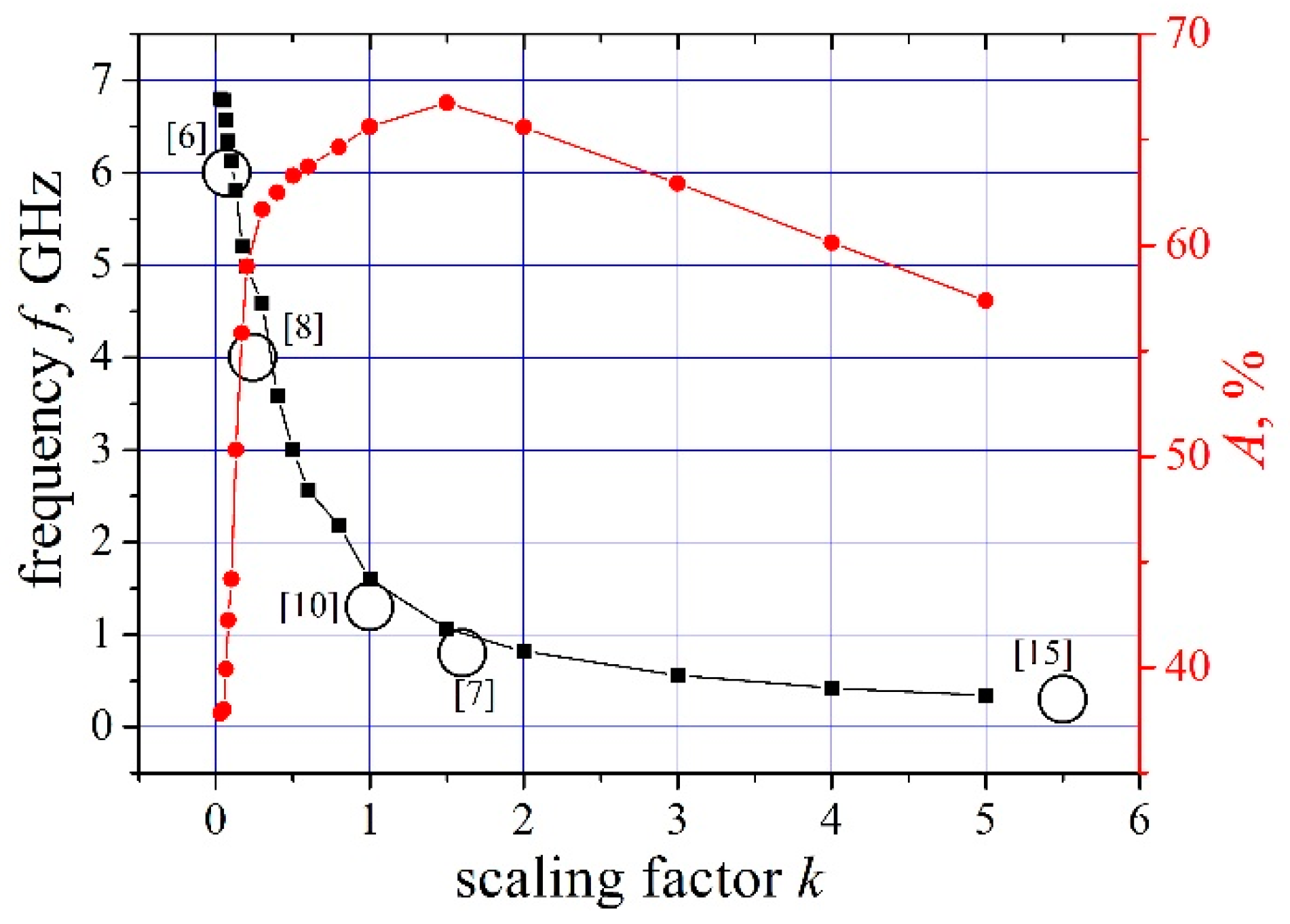
Figure 4.
Calculated oscillation frequency and relative amplitude as functions of the ferrite outer diameter D2 (with D3 = 52 mm).
Figure 4.
Calculated oscillation frequency and relative amplitude as functions of the ferrite outer diameter D2 (with D3 = 52 mm).

Figure 5.
The oscillation frequency and relative amplitude as functions of the coax external diameter D3 (with D2 = 32 mm)
Figure 5.
The oscillation frequency and relative amplitude as functions of the coax external diameter D3 (with D2 = 32 mm)
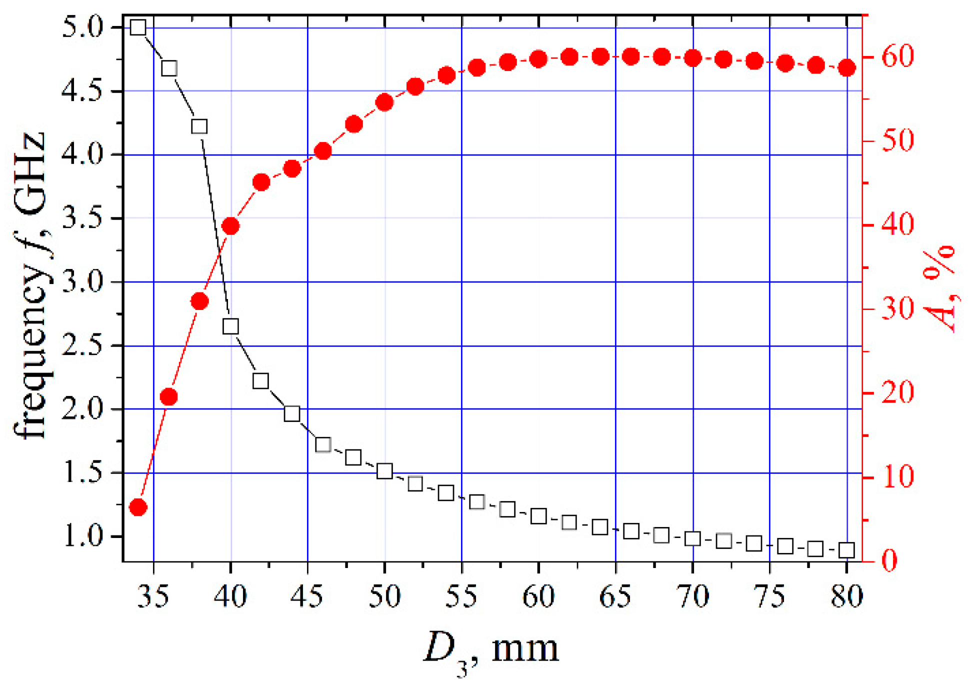
Figure 6.
(a) Model I: output waveforms of a pulse with initial rise time tr = 0.8 ns (curve 1) in TLs of different lengths, L = 200 mm (curve 2), L = 500 mm (curve 3), and L = 800 mm (curve 4); (b) Model II: output waveforms of a pulse with tr =2 ns (curve 1) in TLs of different lengths, L = 200 mm (curve 2), L = 500 mm (curve 3), and L = 800 mm (curve 4).
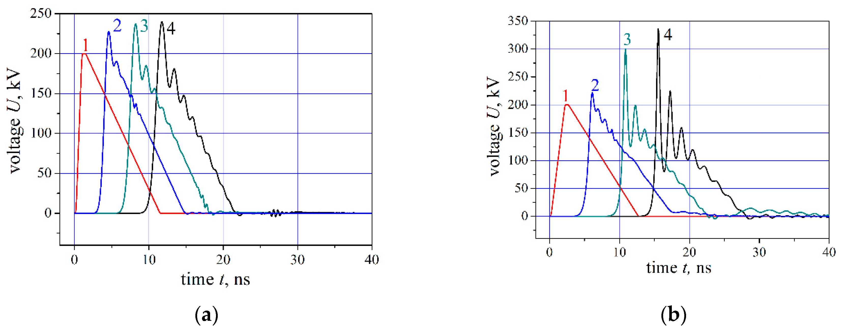
Figure 7.
Model I, linear: field intensity presentations of the Eρ, Hφ, and EZ components in a ‘triangular’ pulse form.
Figure 7.
Model I, linear: field intensity presentations of the Eρ, Hφ, and EZ components in a ‘triangular’ pulse form.
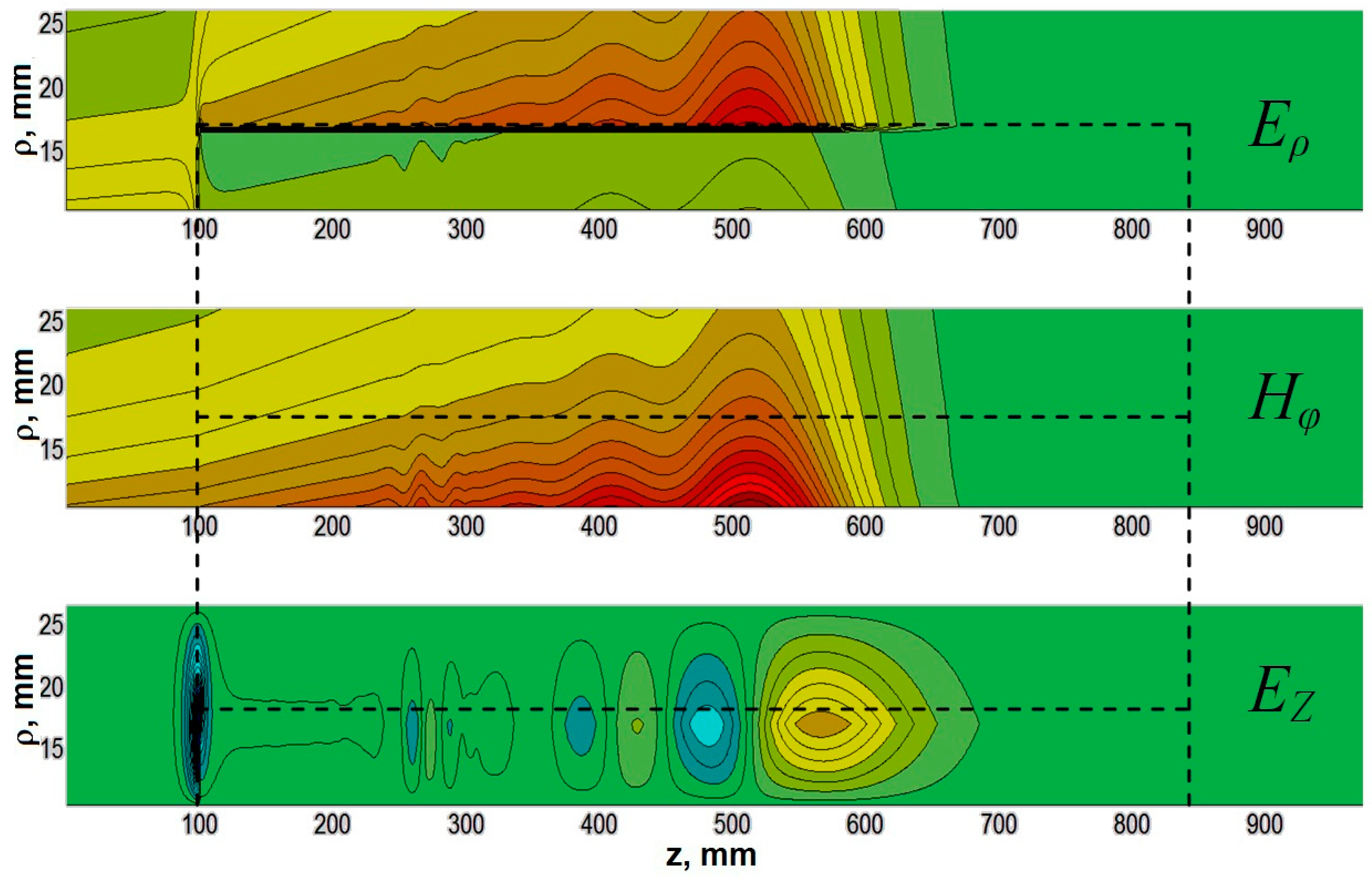
Figure 8.
Model II, nonlinear and isotropic: field intensity representations of the Eρ, Hφ, and EZ components in a ‘triangular’ pulse form.
Figure 8.
Model II, nonlinear and isotropic: field intensity representations of the Eρ, Hφ, and EZ components in a ‘triangular’ pulse form.

Figure 9.
Model III: output waveforms of a pulse with tr = 2 ns at the input (curve 1) in TLs of different lengths, viz. L = 200 mm (curve 2), L = 500 mm (curve 3), and L = 800 mm (curve 4).
Figure 9.
Model III: output waveforms of a pulse with tr = 2 ns at the input (curve 1) in TLs of different lengths, viz. L = 200 mm (curve 2), L = 500 mm (curve 3), and L = 800 mm (curve 4).

Figure 10.
Model III, nonlinear and gyrotropic: field intensities of the Eρ, Hφ, and EZ components as developed from the initial ‘triangular’ pulse form (cf. Figure 8).
Figure 10.
Model III, nonlinear and gyrotropic: field intensities of the Eρ, Hφ, and EZ components as developed from the initial ‘triangular’ pulse form (cf. Figure 8).
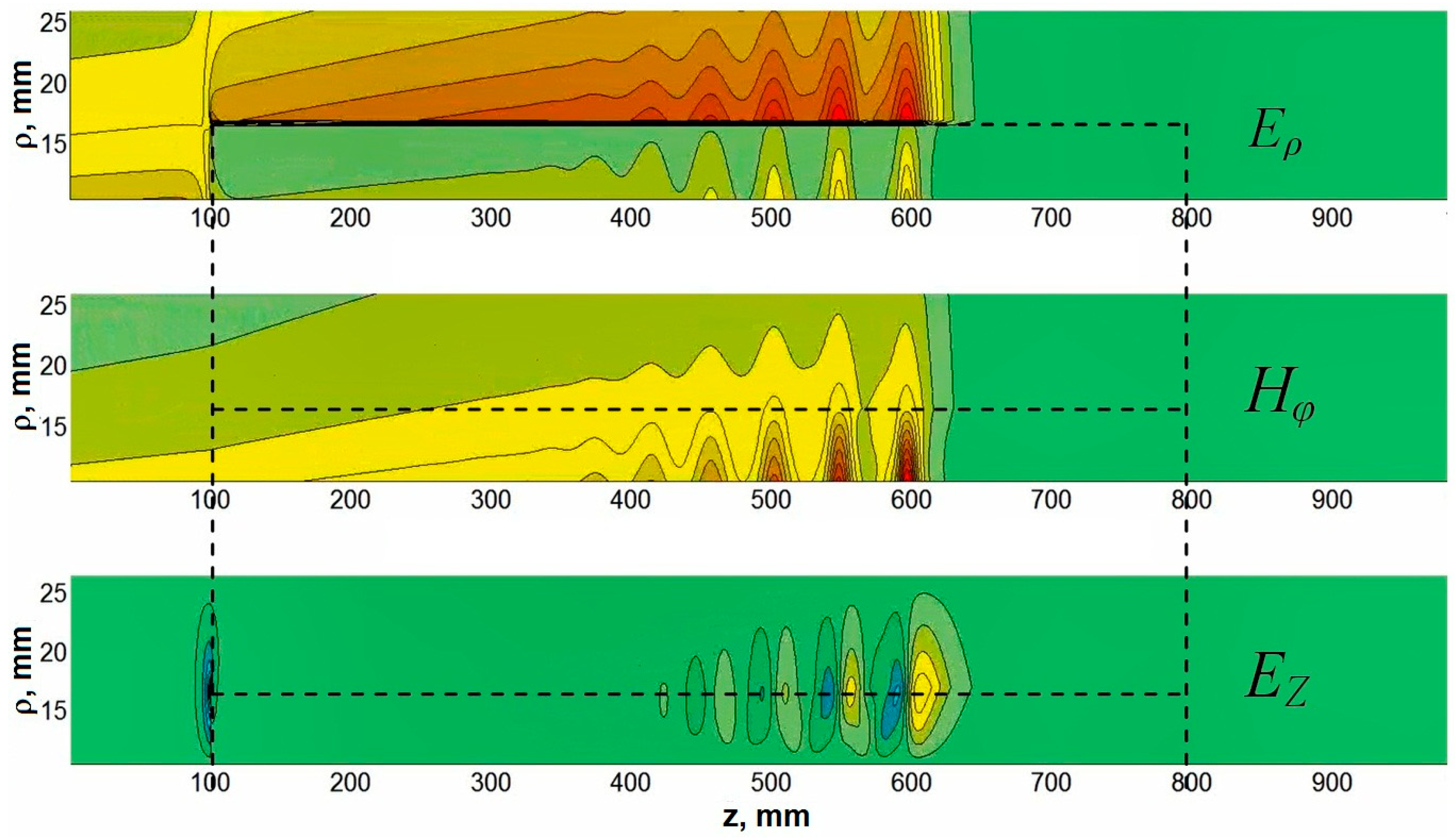
Figure 11.
Pulsed waveforms at the output of NLTLs of different lengths in the case of a structure with ε1 = 80 (slow-down layer): (1) L = 400 mm; (2) L = 800 mm; (3) L = 1200 mm, and (4) L = 1600 mm.
Figure 11.
Pulsed waveforms at the output of NLTLs of different lengths in the case of a structure with ε1 = 80 (slow-down layer): (1) L = 400 mm; (2) L = 800 mm; (3) L = 1200 mm, and (4) L = 1600 mm.

© 2019 by the authors. Licensee MDPI, Basel, Switzerland. This article is an open access article distributed under the terms and conditions of the Creative Commons Attribution (CC BY) license (http://creativecommons.org/licenses/by/4.0/).
Share and Cite
MDPI and ACS Style
Karelin, S.Y.; Krasovitsky, V.B.; Magda, I.I.; Mukhin, V.S.; Sinitsin, V.G. Radio Frequency Oscillations in Gyrotropic Nonlinear Transmission Lines. Plasma 2019, 2, 258-271. https://doi.org/10.3390/plasma2020018
AMA Style
Karelin SY, Krasovitsky VB, Magda II, Mukhin VS, Sinitsin VG. Radio Frequency Oscillations in Gyrotropic Nonlinear Transmission Lines. Plasma. 2019; 2(2):258-271. https://doi.org/10.3390/plasma2020018
Chicago/Turabian StyleKarelin, Sergey Y., Vitaly B. Krasovitsky, Igor I. Magda, Valentin S. Mukhin, and Victor G. Sinitsin. 2019. "Radio Frequency Oscillations in Gyrotropic Nonlinear Transmission Lines" Plasma 2, no. 2: 258-271. https://doi.org/10.3390/plasma2020018