The coaxial structure used in our (and other) experiments (
Figure 1) will be described in a cylindrical frame of reference (
z, ρ, φ), where
z is the coordinate along the line’s axis;
ρ the radial, and
φ the angular coordinate. It involves two uniform lines, TL1 and TL2, at the input and output, respectively, and the line NLTL that is partially filled with a ferrite. In recent studies by the present writers [
10,
11,
12] the cross-section sizes of all three TLs were the same,
D3 = 52 mm and
D1 = 20 mm, which figures determined a 38 Ohm impedance for the TEM mode, and the lengths were 1000 mm for TL1 and TL2, and 800 mm for the NLTL. The TL1 and TL2 lines were fully filled with an isotropic dielectric with constant parameters (e.g., permeabilities
ε = 2.25 and
μ = 1, like in [
10]), whereas in the NLTL the filling medium occupied two layers. The outer one,
D2/2 ≤ ρ ≤ D3/2, contained the same dielectric as TL1, while the space
D1/2 ≤
ρ ≤ D2/2 accommodated a cylindrical ferromagnetic core with
D2 = 32 mm (actually, a set of closely spaced ferrite beads). The entire structure was placed in a DC magnetic field
H0 =
ezH0 provided by an external solenoid. The geometric and electrical parameters of the similar structures employed by other workers, such as line diameters
D, lengths
L, magnitudes of
ε and
μ, and the pre-magnetizing (bias) field
H0 [
6,
7,
8,
9,
15], were rather different. So, to compare and interpret the reported results it may prove expedient to suggest some scaling parameter, introducing an effective uniformity of the electromagnetic conditions. A variant of using such scaling parameter,
k, is described in
Section 3.2 below. It assumes a proportional variation of the waveguide’s transverse dimensions
D′i =
Di/
k, and the pulsed voltage at the line’s input,
U′ =
U/k.
2.1. Wave Modes
The processes taking place in the system can be outlined as follows. The unipolar voltage surge fed into TL1 from an external pulse-forming source travels toward the front edge of the NLTL. The angular uniformity of the geometry suggests periodicity of the field distributions throughout, such that field magnitudes registered at
φ =
φ0 +
2π shall be equal to the relevant values at
φ = φ0, and hence the angular dependences of the wave fields be
exp(
inφ) with
n = 0, ±1, ±2, etc. In spectral terms, the wave fields represent infinite sets of harmonic components,
ΣCnRn(
ρ)expi(
nφ+ωt-κz)d
ω, where
κ is the propagation constant and
Cn and
Rn are, respectively, the amplitude and the radial distribution function in the
n-th component of a specific field vector, at a frequency
ω. The incoming frequency spectrum extends from ‘almost DC’ to 1/
tr, where
tr is the pulse’s rise time. The highest frequency in the set determines the ‘sharpness’ of the pulsed waveform edge. The lowest, of amplitude
C0 about
U0/(
D3−
D1) carries the major part of the pulse’s energy (
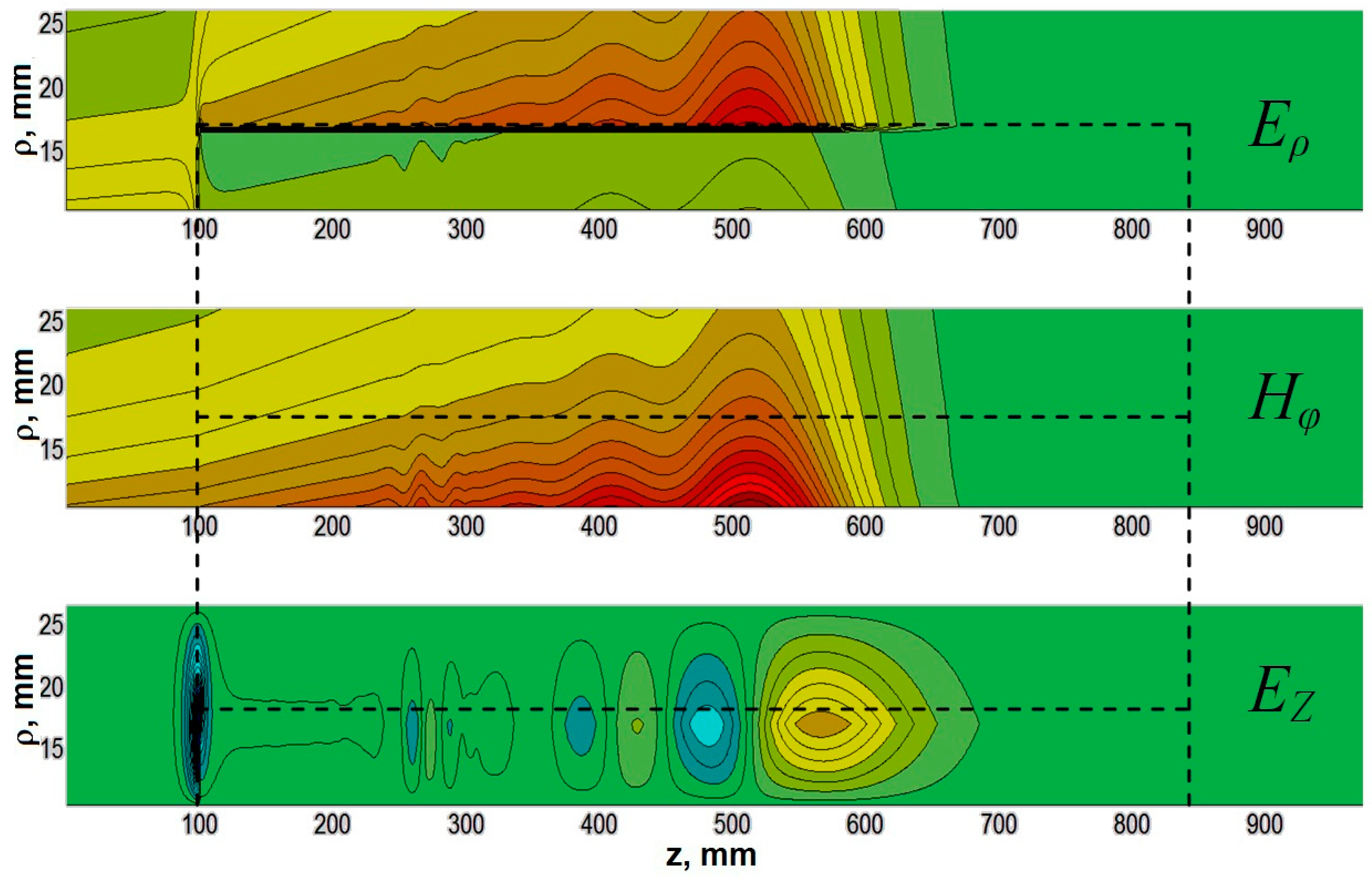
U0 is the peak voltage amplitude of the pulsed waveform). Since the input line, TL1, involves no structural non-uniformity or anisotropy, the ‘DC’ pulse may travel through it in the form of a ‘dispersionless’ (TEM) mode where its participating spatial components are, by virtue of excitation, only two, namely the radial electric,
Eρ (associated with the voltage across the line conductors) and the azimuthal magnetic
Bφ =
Hφ, proportionate to the current through the line. The TEM mode is characterized by the angular uniformity
∂/
∂φ =
in = 0, such that all frequencies travel at the same speed. Accordingly, the term ‘dispersionless’ just means that all frequency components obey the same linear dispersion law
ω = κv. Upon entering the ferrite-filled part of the line the signal can no more exist as a wave packet wherein all frequency components belong to a spatial mode with the same dispersion law
ω =
ω(
κ). First, because any wave mode with non-zero
Eρ and
Bφ gets diffracted at the dielectric-ferrite interface (where the electric and the magnetic parameters of the medium change abruptly), and hence acquires longitudinal components,
Ez and
Bz, which the initial
Eρ and
Bφ are coupled to through the Maxwell equations, e.g.,
Here, the magnetic inductance is
B =
μ0 (
H+
M), with
M being the magnetization vector and
μ0 the permeability of free space. As concerns electromagnetic excitations, the
n = 0 (TEM) mode is not the only solution that can be excited here. The modes with │
n│ ≥ 1 may involve more (up to all six) spatial field components, posing as hybrid EH or HE modes, and possess different, often intricate dispersion laws. The
n = 0 mode itself transforms into a TM mode with three spatial components,
Eρ,
Bφ, and
Ez, and reveals a slightly nonlinear dispersion law [
18]. (For this reason, it is sometimes called the ‘quasi-TEM’ mode). The full set of wave modes supported by the transmission line is determined by its dispersion properties which are dictated by the line’s geometry and size and the type of constituent relations for the filling material. The dynamics of variations in
M can be described with the phenomenological Landau–Lifschitz (L-L) equation, e.g., taken in Gilbert’s form [
19]
which just provides the constituent relation
B =
B(
H). Here
γ = 2.8 × 10
10 Hz/T is the gyromagnetic ratio and
H denotes the total magnetic field in the medium. The magnetic field
H in Equation (1) is to be estimated from the Maxwell equations, with due account of all boundary conditions for the
E and
B fields, so as to ‘automatically’ involve the so called de-magnetizing terms owing to finite sizes of the ferrite beads and the core as a whole [
19]. Next,
α < 1 is a phenomenological parameter of this macroscopic equation, accounting for magnetic relaxation effects.
Considering the pulse propagation through the line we assume that the ferromagnetic core was initially magnetized by the DC field H0 almost to the saturation level M0 = ezMs. Now it is re-magnetized under the impact of the perpendicular field eφHφ which is produced by the z-oriented pulsed current. That field may be represented as Hφ = H0φ + hφ(t), where H0φ is a ‘nearly DC’ component of the incoming pulse, of a frequency about 1/τ with τ being the total pulse duration, such that H = ezH0 + eφH0φ + h(t). Accordingly, the magnetization vector M acquires spatial components oriented along the ρ-, φ-, and z-directions, both static and varying with non-zero frequencies. The variations of Mρ and Mφ with time represent the precession motion of M around the direction of the total magnetic field H.
As can be seen from Equation (1), the B = B(H) relation is (a) nonlinear and (b) anisotropic. Qualitatively, the effects of magnetic nonlinearity can be described in two ways:
1. By introducing an ‘effective magnetic permeability’ of the ferrite along the z-axis, which would be dependent on the magnetic field strength, for example like μ = 1 + M(H)/H. Within this approach, the propagation velocity v = c(εμ)−1/2 of the pulsed wave is treated as dependent on the amplitude of Hφ (i.e., current amplitude). As a result, the higher-amplitude pulse components run in advance of the lower-amplitude ones, thus sharpening the front edge and provoking shock formation. Of course, this is a rather simplified treatment, as the M = M(H) and, hence B = B(H) are not scalar relations. The refractive index c/v can hardly be associated with any scalar ‘effective μ’.
2. By considering the pulse propagation as a process of spectrum transformation and mode conversion along the line. Then the Maxwell set and the L-L-G Equation (1) need to be brought to the frequency-domain representation,
where
δ(
ω −
ω′), etc., is Dirac’s delta. The coupling of the magnetization vector’s frequency components owing to nonlinearity becomes explicitly evident. Accordingly, the formerly independent eigenmodes specified by the linear-approximation solutions for the
E and
B fields get coupled, too. A linear in
h solution to Equation (3) yields the familiar magnetic permeability tensor
μ [19]. With regard to pulse propagation, a major effect of nonlinearity is generation of higher-order harmonics by each component from the continuous spectrum presented by the pulse. As long as they all travel, within the TEM mode, at nearly equal phase velocities (close to the pulse’s group velocity
vg), we observe sharpening of the pulse’s edge. When some of the higher frequency components gets close to and beyond the cut-off frequency,
fcr, for a dispersive TM, TE or a hybrid mode potentially supported by the line, that wave mode may be excited and then run downstream the line at its phase velocity
vph. If the excited mode were faster than the shock wave (
vph >
vsh), it would be seen as a decaying sine waveform. The rate of decay might be reduced or even replaced by amplification, should the wave happen to be in a velocity synchronism with its coupled partner. That is another important effect owing to nonlinearity.
The linear in
h(
ω) solution to the L-L-G+Maxwell equation set representing the magnetic wave in the ferrite also looks like a decaying sine wave, which has led many writers (e.g., [
6,
8,
9,
13,
15,
20]) to believe that the arising oscillations are associated exclusively with precession of the magnetization vector. However, the latter is often estimated for a boundless specimen of the ferromagnetic material, without account of demagnetization effects [
13,
20]. Meanwhile, the frequency of magnetic moment precession is not the only characteristic frequency in the structure. The NLTL, as a line of finite-sized cross-section (and containing a layered insert at that) may support linear-approximation modes obeying a variety of dispersion laws that may involve cut-off frequencies, unlike the TEM mode. The electromagnetic eigenmode frequencies are given by a secular equation following from the full set of Maxwell equations, with proper boundary conditions and constituent relations, rather than the equation of motion for the
M-vector alone. The cut-off frequencies are determined by transverse dimensions of the guiding structure. The description of the precession motion of
M involves magnitudes like
ω0 =
μ0γH
0,
ωM =
μ0γMs, and
ωφ =
μ0γH0φ. In a number of experiments (e.g., [
6,
8,
13,
15]), the corresponding frequencies
f0,
fM, etc., lay below 1 GHz (with
H0 ranging from about 10 kA/m to 30 kA/m), while the recorded oscillation frequencies were between 0.3 GHz and 6 GHz. In fact, the magnitudes
ω0,
ωM etc, each having the dimension of frequency, appear in the form of combinations
ω0 +
ωM, (
ω2 −
ω02), etc., in frequency-domain solutions for components of the magnetic permeability tensor (see [
19]) that determine variations in the magnetization vector
M. Note that in every specific experiment
H0 stayed constant, whereas
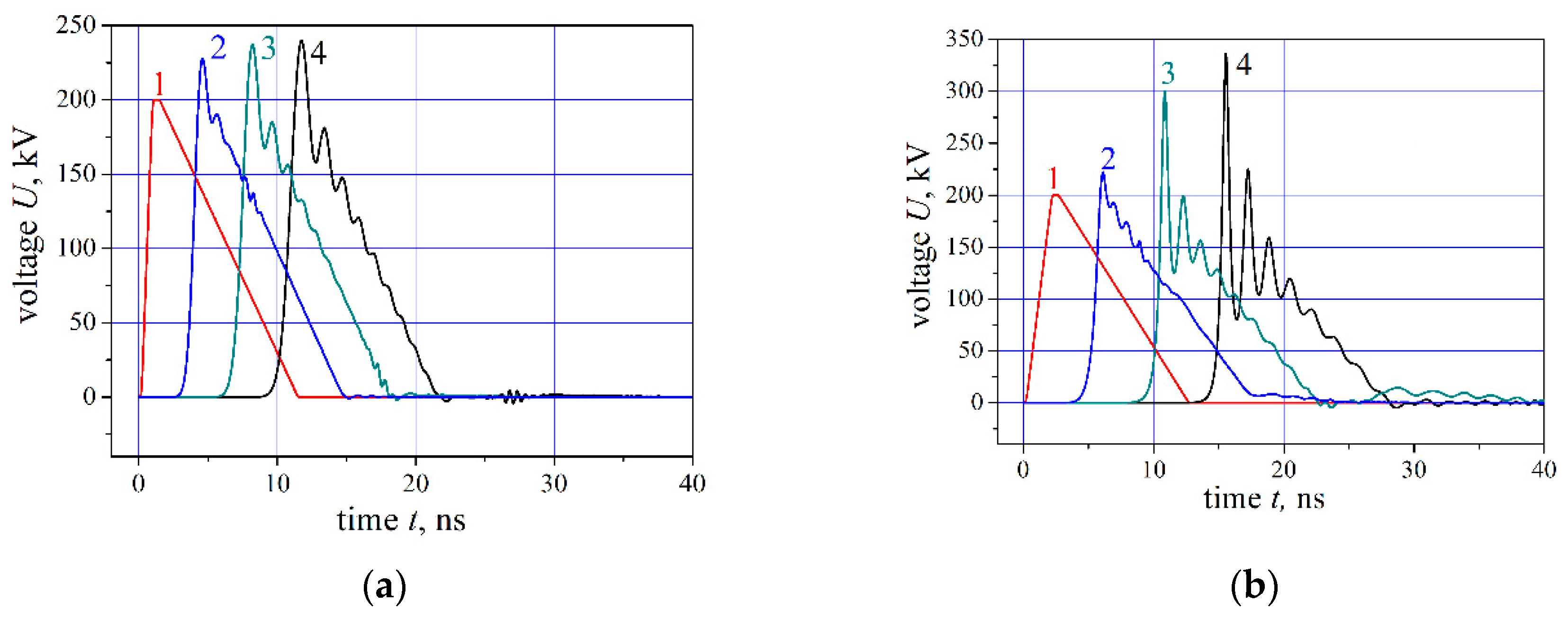
Hφ changed noticeably over the duration of the current pulse. A series of experiments and simulations [
11,
12,
14] performed with ‘triangular’ pulse waveforms (see below,
Figure 2) are, in this respect, of special interest. Throughout the extended trailing edge, the magnitude of
Hφ changes by a factor greater than 10, while the RF oscillation frequency never varies by more than 15%...25%. This small amount of frequency variations, compared with the greatly changing pulse amplitude, apparently suggests a rather low significance, under the conditions of a specific experiment, of the magnetic state of the medium, i.e., of magnetization dynamics. Then we have to admit that the oscillation frequency is not (at least, not always is) related as tightly to the
M-vector precession.
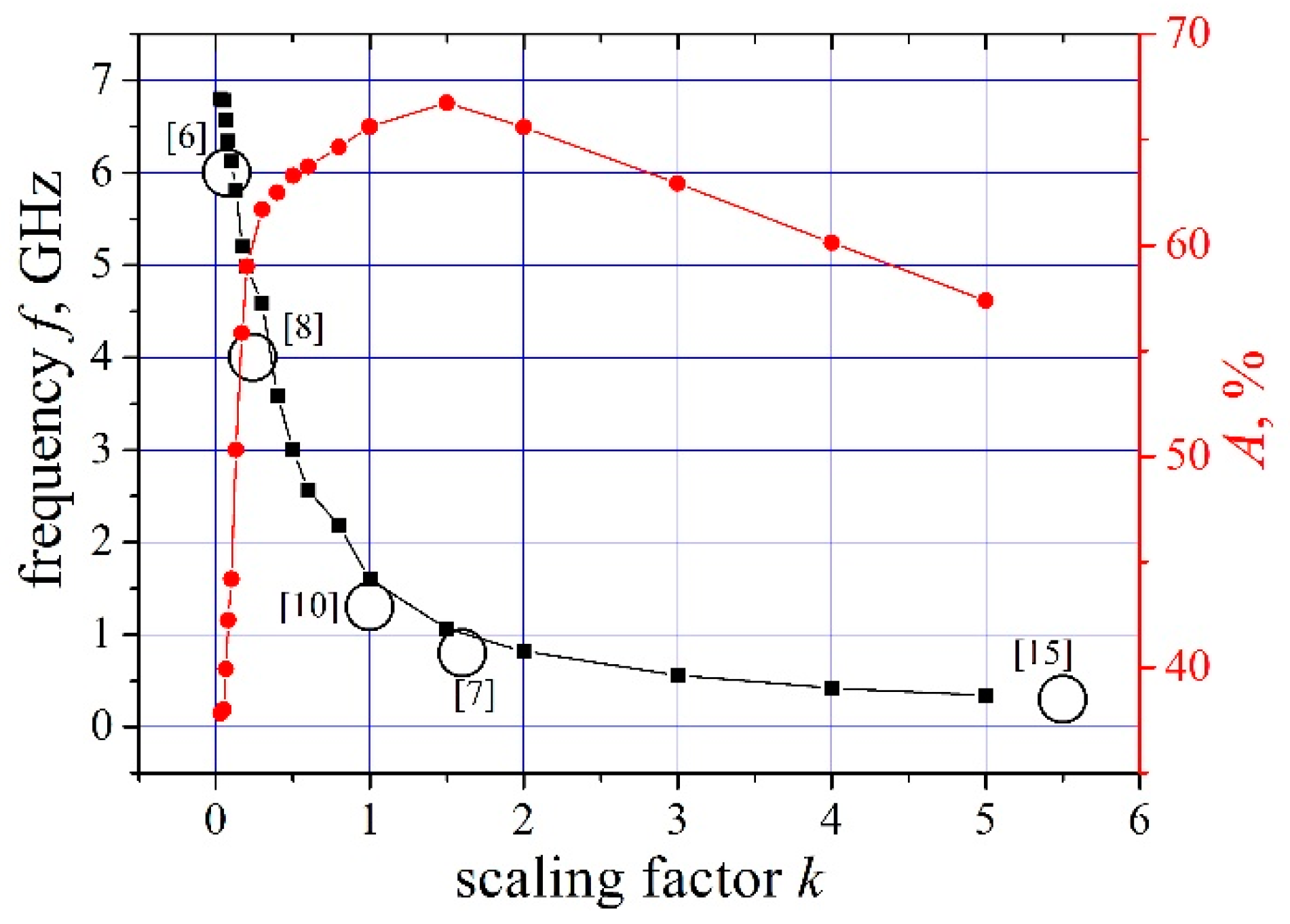
2.2. Size Dependences
As an alternative, consider the dependences upon sizes of the structural elements. The great many experiments with nonlinear TLs, showing a variety of outer diameters
D3, sizes of the ferrite beads, and magnitudes of the magnetic fields, allow bringing their results on the oscillation frequency
f to the general form
f~
D−1. Thus, Dolan [
6] operated with coaxial lines of very small diameters (
D3 ≈ 3 mm) and observed oscillations at a high frequency
f ≈ 6 GHz. A series of real-life experiments [
7,
8,
9] and numerical simulations [
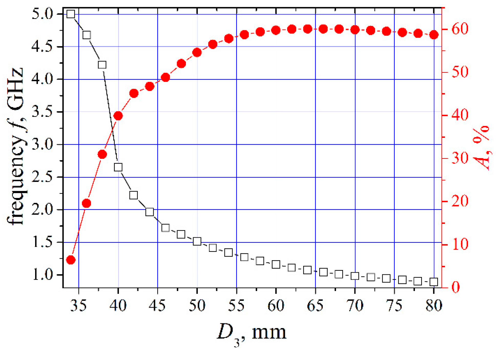
12] performed with a variety of NLTL diameters revealed good agreement between the frequency vs. size relation and the formula
f~
D−1. With the diameters
D3 varying from 20mm to 50 mm the oscillation frequencies changed between 2.3 GHz and 0.9 GHz. Gubanov et al. [
7] experimented with lines of a large diameter ~80 mm and observed oscillations at lower frequencies (0.8 GHz…2 GHz). Finally, the writers [
15] employed TLs of a still larger diameter (275 mm) and obtained a much lower frequency,
f~0.3 GHz. The relationship between the oscillation parameters and transverse dimensions of the NLTL is shown in
Figure 3 as dependences of the oscillation frequency and relative amplitude,
A = (U1 − U2)/(U1 + U2), upon the scaling factor
k. This latter assumes a proportional variation of the waveguide’s transverse dimensions
D′i =
Di/
k, and the pulsed voltage at its input,
U′ =
U/k. With this proportion held, the current-induced azimuthal magnetic field
Hφ re-magnetizing the ferrite remains unchanged. The
k = 1 magnitude of the scaling factor relates to the case
D3/
D2/
D1 = 52 mm/32 mm/20 mm. The results of simulations, also presented in
Figure 3, confirm the trend revealed in the experiment, namely that with an increase of the transverse dimensions, the oscillation frequency decreases, whereas their amplitude increases. Details of the computational work, in a version of the FDTD, were earlier described in [
14]. Additionally, it can be seen that with smaller transverse dimensions (smaller
k) the oscillation frequency reaches a certain high level where it almost stops changing further. Thus, both experiments and numerical calculations indicate that the oscillation frequency is, more often than not, related to transverse dimensions of the coaxial NLTL, while its relation to magnetization parameters (the bias field in particular) is not straightforward.
