Investigation of Variability of Flaw Strength Distributions on Brittle SiC Ceramic

Abstract

The present paper investigates flaw strength distributions established using various flexural tests on batches of SiC bar test specimens, namely four-point bending as well as three-point bending tests with different span lengths. Flaw strength is provided by the elemental stress operating on the critical flaw at the fracture of a test specimen. Fracture-inducing flaws and their locations are identified using fractography. A single population of pores was found to dominate the fracture. The construction of diagrams of p-quantile vs. elemental strengths was aimed at assessing the Gaussian nature of flaw strengths. Then, empirical cumulative distributions of strengths were constructed using the normal distribution function. The Weibull distributions of strengths are then compared to the normal reference distributions. The parameters of the Weibull cumulative probability distributions are estimated using maximum likelihood and moment methods. The cumulative distributions of flexural strengths for the different bending tests are predicted from the flaw strength density function using the elemental strength model, and from the cumulative distribution of flexural strength using the Weibull function. Flaw strength distributions that include the weaker flaws that are potentially present in larger test pieces are extrapolated using the p-quantile diagrams. Implications are discussed regarding the pertinence of an intrinsically representative flaw strength distribution, considering failure predictions. Finally, the influence of the characteristics of fracture-inducing flaw populations expressed in terms of flaw strength interval, size, dispersion, heterogeneity, and reproducibility with volume change is examined.

1. Introduction

Microstructural flaws that act as stress concentrators cause the fracture of many brittle materials, including ceramics. The flaws generated during the manufacturing of ceramic and glass pieces are generally distributed randomly, and they may exhibit wide variability in severity as a result of the variability in shape, nature, and size. As a consequence, a stress-induced fracture is a stochastic event, and fracture stress is a variate. The strength of brittle ceramics is commonly characterized by statistical distribution functions, which allows the interpretation of strength variability and the prediction of component reliability.

The statistical variability of ceramic strength is commonly characterized by the Weibull distribution function, which is based on a power law. Then, statistical-probabilistic approaches can be used to assess the fracture stress of specimens or components containing flaws. For this purpose, they should enable the use of laboratory data to infer the probability of a fracture of a component under the more complicated stress states encountered in service (nonuniform polyaxial stress states, transient stress states), which requires considerable extrapolation to larger sizes, as well as to more complex stress states than those encountered with the specimens usually tested under uniaxial stresses. Therefore, appropriate distribution functions and statistical-probabilistic approaches are required to describe specimen size effects on strength.

According to Weibull, “the only merit of the distribution function he proposed, is to be found in the fact that it is the simplest mathematical expression of the appropriate form, which satisfies the necessary general conditions” [1]. However, authors raised questions about the validity of the Weibull distribution for ceramic strengths, owing to the variation in the estimated statistical parameters and the bias introduced via the method of the estimation of Weibull parameters [2,3,4,5,6,7,8,9,10]. They have compared various distribution functions, and no consensus has emerged on the proper form. Thus, for instance, an outcome of the detailed statistical analysis of the flexural strength data [11] using various probability models, including Weibull, normal, log-normal, gamma, and generalized exponential distributions, was that the gamma or log-normal distribution function, in contrast to the Weibull distribution, may describe more appropriately, in certain cases, the experimentally measured strength data. The normal distribution was assumed by a few researchers on bulk ceramics and ceramic fibers [11,12,13,14,15,16]. However, it was also reported that the fitted Weibull and normal distributions of flexural strengths behave quite similarly [11,12]. The similarity of normal and Weibull distributions has also been established on fiber tows made of very large numbers (up to more than 1000) of filaments [15,16].

It is difficult to decide whether the strength data follow a Weibull distribution or not when small sample sizes and a single batch of specimens of the same dimensions are considered. The validity of a distribution function implies that the statistical parameters are constant whatever the specimen size and the stress state. In the case of small diameter ceramic fibers tested under a tensile load, the estimated Weibull parameters pertinent to flaw strengths display variation depending on various factors, including the methods of analysis of experimental strength data [15,16,17], the sample size, and also the selection of test specimens (sampling) from a tow [15,16]. Sampling dictates the populations of critical flaws present in the tows. As reported in [18], authors did not agree on the most appropriate method of accurately determining the Weibull distribution function for brittle materials.

In a recent paper on ceramic fibers [16], it was shown that the linearity of the p-quantile vs. flaw strength relation indicates that the critical flaw strength in a fiber tow is a Gaussian variable. This approach was applied to various fiber types, including SiC, carbon, glass, basalt, and alumina fibers [16], to construct empirical flaw strength distributions. It was shown to avoid some of the above sources of bias for the estimation of the Weibull statistical parameters [16]. This approach was applied to a monolithic ceramic in the present paper.

There are two main types of probabilistic-statistical approaches to predict the fracture stress of specimens or components containing flaws [2] as follows:

• The phenomenological and macroscopic approaches which consider specimen strengths, like the Weibull model;
• The approaches that consider the flaws as physical entities [2,19,20,21,22,23,24,25]. They are more fundamental. They are based on the flaw strength density function. The severity of a flaw is measured either using the flaw strength or flaw size. The flaw strength is defined as the critical value of the local stress operating on a volume element containing a single flaw (also referred to as elemental stress) that causes the extension of the flaw. The failure probability of a test piece is derived from the flaw strength density function using the following equation [21,22,23,24,25]:

$$P=1-\mathrm{e}\mathrm{x}\mathrm{p}\left[-\int dV{\int }_0^{S}g\left(S\right)dS\right]$$

(1)

where g(S) is the flaw strength density function, S is the elemental strength, and V is the stressed volume.

A power law equation is generally selected for g(S) because it can be integrated easily for the calculation of probability using Equation (1). The determination of the parameters of the power law requires the experimental distribution of flaw strengths. However, unlike fibers, the determination of this empirical distribution of flaw strength is not straightforward for bulk ceramics since tensile tests are precluded due to practical difficulties. Bending tests are commonly used on ceramics. Therefore, most analyses and predictions of strength distributions are based on specimen strength data (macroscopic approach), neglecting the sources of fracture (the microstructural flaws). The approach proposed in the present paper is different in essence since the strength of the fracture-inducing flaws was considered. The location of critical flaws was identified, and the flaw strength was derived from the measured data.

The present paper investigates flaw strength distributions in a bulk SiC ceramic, with the intent to propose an approach based on p-quantile diagrams to anticipate specimen size effects on the flaw strength density function, with the aim of predicting the specimen strength using the elemental strength model under various stress states and volumes. The Weibull distributions of the flaw and flexural strengths were considered for comparison purposes.

2. Materials and Methods

Flaw strengths were determined using flexural tests on SiC bending bars and fractography. The construction of p-quantile diagrams allowed the normal distribution to be assessed, which permitted the construction of unbiased cumulative distribution functions (CDFs) and probability density functions (PDFs). The Weibull distribution function was then compared to the reference normal distribution. A power law for g(S) was derived from four-point bending tests. The flexural strength distributions at different 3pt bending conditions were then predicted using Equation (1) and the Weibull equation. Then, broader flaw strength distributions that incorporate potential weaker flaws that were not present nor activated due to their location with respect to the stress gradient in bending bars were constructed using the p-quantile diagrams.

2.1. Generation of Flaw Strength Data

Three- and four-point bending fracture tests were conducted on sintered silicon carbide bars at a constant displacement rate of 1 mm/min. A servohydraulic Instron machine was used. Long and short span lengths were selected for the 3-point bending tests in order to vary the stressed volume. The long spans induce a predominantly uni-axial stress state, whereas appreciable shear stresses may exist in the section of the short span specimens.

The bar specimens were machined out of plates having dimensions of 40 × 40 × 10 mm³. The 3 batches of 70 bar test specimens comprised specimens from the different plates. After machining, all the specimens were beveled and polished on the opposite faces using diamond disks. The specimen dimensions are given in

Table 1. Test specimen dimensions.

	Length (mm)	Thickness 2d (mm)	Width b (mm)	Upper Span 2l1 (mm)	Lower Span 2l (mm)
3pt long span	45	4	4	0	40
3pt short span	20	4	4	0	10
4pt	45	4	4	20	40

.

The stresses at the fracture origins (flaw strengths) were derived from the maximum stress as follows:

$$\text{-3-point bending}:{\sigma }_z={\sigma }_{max}\left(\frac{l-z}{l}\right)\left(\frac{x}{d}\right)$$

(2)

where σ_z denotes the stress parallel to the longitudinal axis Oz at the flaw location, σ_max is the maximum stress in the outer surface ${\sigma }_{max}=\frac{3Fl}{4b{d}^2}$; x is the distance from the neutral plane, 2d is the specimen thickness, z is the distance from the loading plane, and 2l is the span length.

$$\text{-4-point bending}:{\sigma }_z={\sigma }_{max}\left(\frac{x}{d}\right)$$

(3)

where σ_z denotes the stress at the flaw location parallel to the longitudinal axis Oz between the loading pins, σ_max is the maximum stress in the outer surface between the loading pins ${\sigma }_{max}=\frac{3F{l}_2}{4b{d}^2}$, l₂ = l − l₁, x is the distance from the neutral plane, and 2d is the specimen thickness.

Fracture mirrors showed the locations of fracture-inducing flaws. The plane of fracture origin was always perpendicular to the σ_z direction. Processing flaws consisting of pores dominated the fracture (>91%). The strengths of the other flaw types were distributed evenly. Therefore these data were kept. Figure 1 shows an example of pore fracture origin identified in the fracture surface of a 3pt bending specimen. Fractographic analysis showed that fracturing occurred always in the central loaded region of specimens, perpendicular to the direction of longitudinal tensile stress σ_z. For the 4point bending specimens, it occurred in the part of the specimens located between the loading pins and close to the outer surface. Therefore, for the 4pt bending tests, the flaw strengths coincided with the flexural strengths.

2.2. Analysis of Flaw Strength Data

2.2.1. p-Quantile Diagrams and Normal Distribution [16]

The approach based on the p-quantile diagram was proposed in a previous paper to demonstrate that the filament flaw strength is a Gaussian variable [16]. It is a graphical method for comparing a Gaussian distribution to a set of data. When X is a Gaussian variable, with μ = mean, s = standard deviation, and N is a variable of the standard normal distribution, the following is true:

$$P\left(X<x\right)=P\left(\frac{X-\mu }{s}<\frac{x-\mu }{s}\right)=P\left(N<z\right)=\mathsf{\Phi }\left(z\right)$$

(4)

where P (.) is probability,

$$z=\frac{x-\mu }{s}$$

(5)

and Φ is the cumulative standard normal distribution of variable z.

Thus, when the linearity of the relation z(x) (Equation (5)) is observed for a set of x_i data, one may assume that the x_i data are occurrences of the same Gaussian variable. Then, the plot of the p-quantile z_p vs. σ_p indicates whether the strength is a Gaussian variable.

$$z_p={\mathsf{\Phi }}^{-1}\left(p\right)=\frac{{\sigma }_p-\mu }{s}$$

(6)

where p = i/(n + 1). z_p can be extracted easily from Φ using a computer or tables available in text books.

2.2.2. Analysis Using the Normal Distribution

The reference CDFs were calculated using the cumulative normal distribution function (Equation (7)) for the values of the mean μ and standard deviation s of the sets of experimental strength data as follows:

$$P_n\left(\sigma \right)=\frac{1}{s\sqrt{2\pi }}{\int }_0^{\sigma }\mathrm{e}\mathrm{x}\mathrm{p}(-\frac{{(t-\mu )}^2}{2s^2})dt$$

(7)

The normal CDFs are referred to as reference distributions because they provide unbiased graphical representation of the empirical distribution, unlike the Weibull plot.

2.2.3. Analysis Using the Elemental Strength Model

The equation of the elemental strength model relates probability to flaw strength density via Equation (1). This equation was used to calculate probabilities under the various bending conditions. As detailed in [2], after the introduction of the power law expression of g(S), Equation (1) becomes

$$P=1-\mathrm{e}\mathrm{x}\mathrm{p}[-\frac{1}{V_0}\int dV{\left(\frac{{\sigma }_1}{S_0}\right)}^{\lambda }\mathrm{I}(\lambda ,\frac{{\sigma }_2}{{\sigma }_1},\frac{{\sigma }_3}{{\sigma }_1}\left)\right]$$

(8)

where σ₁, σ₂, σ₃ are the principal stresses and λ and S₀ are statistical parameters. I(.) is a function of local and principal stresses. In the present bending tests, σ₁ = σ_z, σ₂ = σ₃ = 0; $\mathrm{I}\left(\lambda ,\frac{{\sigma }_2}{{\sigma }_1},\frac{{\sigma }_3}{{\sigma }_1}\right)=\mathrm{I}\left(\lambda ,\mathrm{0,0}\right)$ [2].

After the introduction of S as a function of σ_max (Equations (2) and (3)) into Equation (1), after integration, the following is true:

$$P=1-\mathrm{e}\mathrm{x}\mathrm{p}(-V_E(\lambda \left){I(\lambda ,\mathrm{0,0})\left(\frac{\sigma }{S_0}\right)}^{\lambda }\right)$$

(9)

V_E(λ) results from the integration of Equations (2) and (3). For the 3-point bending specimens,

$$V_E\left(\lambda \right)=\frac{V}{2{(\lambda +1)}^2}$$

(10)

For the 4-point bending specimens,

$$V_E\left(\lambda \right)=\frac{V(\lambda +2)}{2{(\lambda +1)}^2}$$

(11)

V_E(λ) is the statistically equivalent volume, subject to S = σ_z operating uniformly.

2.2.4. Analysis Using the Weibull Model

The Weibull distributions of strength data were calculated using the statistical parameters derived from the experimental strength data. The Weibull distribution functions were compared to the reference normal distribution functions for assessment purposes.

The general equations of the probability density function and cumulative distribution Weibull function are, respectively,

$$f\left(\sigma \right)=\frac{m}{{\sigma }_z}{\left(\frac{\sigma }{{\sigma }_z}\right)}^{m-1}exp\left[-{\left(\frac{\sigma }{{\sigma }_s}\right)}^m\right]$$

(12)

$$P\left(\sigma \right)=1-exp\left[-{\left(\frac{\sigma }{{\sigma }_s}\right)}^m\right]$$

(13)

where m is the Weibull parameter, σ is the strength, and σ_s is the characteristic strength.

For the analysis of the influence of dimensions on strengths, the following equation of the Weibull distribution was used for the flexural tensile stress state:

$$P=1-exp-\left[\int \frac{1}{V_0}{\left(\frac{\sigma }{{\sigma }_0}\right)}^{m}dV\right]$$

(14)

Introducing the expressions (2) or (3) of the stress state and integrating over the stressed volume results in the following:

$$P=1-exp-\left[\frac{V_E\left(m\right)}{V_0}{\left(\frac{{\sigma }_{max}}{{\sigma }_0}\right)}^m\right]$$

(15)

where σ_R = σ_max is the flexural strength of specimens, σ_z is the scale factor, V_E(m) is the above statistically equivalent volume for m and σ_max = σ_z operating uniformly, and V₀ is a reference volume.

The parameters of the Weibull cumulative distribution functions (CDFs) were estimated using the maximum likelihood estimation method and the moment method [18,26,27].

(a)

Maximum Likelihood Estimation (MLE)

The parameter estimates obtained using the maximum likelihood technique are unique (for a two-parameter Weibull distribution), and they are claimed to statistically approach the true values of the population more efficiently than other parameter estimation techniques as the size of the sample increases. They are derived from Equations (16) and (17) as follows:

$$\frac{{\sum }_{j=1}^n{\left({\sigma }_R^j\right)}^{m}Ln{\sigma }_R^j}{{\sum }_{j=1}^n{\left({\sigma }_R^j\right)}^m}-\frac{1}{n}{\sum }_{j=1}^{n}Ln{\sigma }_R^j-\frac{1}{m}=0$$

(16)

$${\sigma }_s={\left[\frac{1}{n}{\sum }_{j=1}^n{\left({\sigma }_R^j\right)}^m\right]}^{\frac{1}{m}}$$

(17)

where ${\sigma }_R^j$ is the jth strength in the set of data.

(b)

Method of moments (MM)

This method has the advantage of involving closed-form equations that can be handled for analytic purposes. The statistical parameters are related to the mean and variance expressions derived from the first moment of the Weibull distribution. The following expressions are used for estimating the Weibull parameters:

$$CV=\frac{s}{\mu }=\sqrt{\left[\frac{\mathsf{\Gamma }\left(1+\raisebox{1ex}{$2$}\!\left/ \!\raisebox{-1ex}{$m$}\right.\right)}{{\mathsf{\Gamma }}^2\left(1+\raisebox{1ex}{$1$}\!\left/ \!\raisebox{-1ex}{$m$}\right.\right)}-1\right]}$$

(18)

$${\sigma }_s=\frac{\mu }{\mathsf{\Gamma }(1+\frac{1}{m})}$$

(19)

where CV is the coefficient of variation and Γ(.) is the Gamma function.

3. Results

3.1. The p-Quantile Diagrams

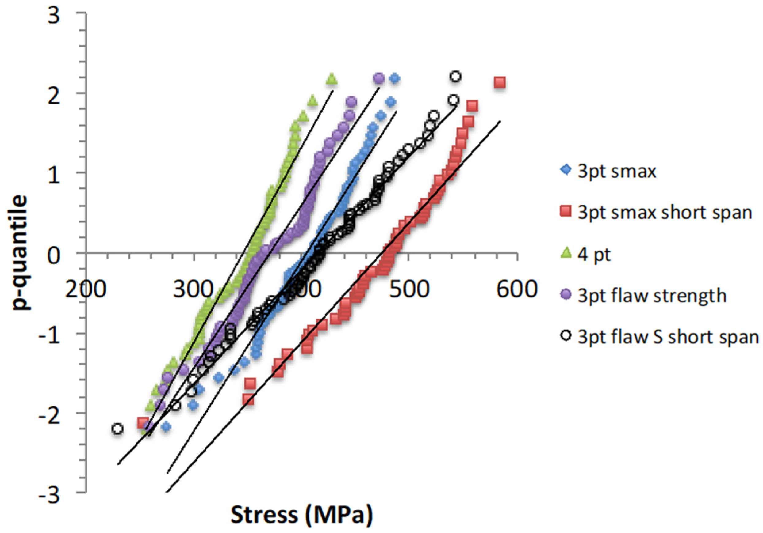
The p-quantile vs. strength diagrams display linearity (Figure 1) with a high value of the correlation coefficient (

Table 2. Coefficients of correlation of p-quantile vs. strengths, normal vs. Weibull cumulative (Pn or PW, respectively), or probability distributions (PDn or PDW, respectively).

	p-Quantile vs. Strength	Pn vs. PW	PDW vs. PDn
4pt	0.985	0.99	0.93
3pt flex strength	0.988	0.997
3pt flex strength short span	0.97	0.997
3pt flaw strength	0.988	0.997	0.90
3pt flaw strength short span	0.99	0.998	0.95
Merged flaw strength	0.995	0.998

). This indicates that the flexural strengths and the flaw strengths follow a normal distribution.

The p-quantile vs. flaw strength diagrams were distinct and depended on the bending mode. It can be noted that the difference between the distributions was larger for the flexural strengths than for the flaw strengths. The increase in the slope of the p-quantile diagrams (=1/s) with increasing V_E indicates that more weak flaws were present in the 4pt bending specimens (larger equivalent volume V_E), whereas stronger flaws were present in the short span 3pt bending specimens (smaller V_E). The long span specimens are an intermediate case. The values of V_E are given in

Table 3. Statistical parameters of the normal and Weibull distributions of the flexural and flaw strengths. Also given are the statistical parameters of the elemental strength model for the 4pt flaw strengths. Also given are the statistically equivalent stressed volumes V_E. Except for the elemental strength model, the parameters of the strength distributions were determined using both MM and MLE methods.

	μ (MPa)	s (MPa)	m Weibull	λ	σs(1) (MPa) Weibull	Scale Factor (MPa) Weibull	S0 (MPa) Elemental Model	VE (10−9 m3)
4pt flaw strength	345.67	38.46	10.9 (MM) 10.8 (MLE)	10.9	362.06 (MM) 362.44 (MLE)	64.9	57	7.29
3pt flexural strength	404.67	44.26	11.1 (MM) 10.97 (MLE)		423.73 (MM) 424,20 (MLE)	66.03		1.09
3pt flexural strength short span	474.27	61.26	9.3 (MM) 9.9 (MLE)		499.23 (MM) 499.0 (MLE)	48.42		0.38
3pt flaw strength	370.3	46.2	9.63 (MM) 9.35 (MLE)		389.82 (MM) 390.1 (MLE)	46.99		1.42
3pt flaw strength short span	414.8	66.55	7.36 (MM) 7.29 (MLE)		442.22 (MM) 442.2 (MLE)	24.54		0.57
Merged flaw strength	377.15	59.12	7.56 (MM) 6.64 (MLE)		401.65 (MM) 402.93 (MLE)	33
extrapolated flaw strength	340	76.92	5.08		369.97
extrapolated flaw strength	295.28	94.34	3.5		328.09

⁽¹⁾ V₀ = 1 m³.

. When the effective volume increased, the high extreme values of the flaw strengths decreased, whereas the low extreme values were quite similar (

Table 4. Values of parameters that define the p-quantile vs. strength diagrams.

	Smin (MPa)	Smax (MPa)	zp	n
4pt flaw strength	256	429	+/− 2.2	69
3pt flexural strength			+/− 2.2	68
3pt flexural strength short span			+/− 2.13	70
3pt flaw strength	259	472	+/− 2.18	68
3pt flaw strength short span	230	544	+/− 2.2	70
Merged flaw strength	230	544	+/− 2.59	207
extrapolated flaw strength	140	544	+/− 2.6	210
extrapolated flaw strength	50	544	+/− 2.6	210

). The p-quantile diagrams of the flaw strengths intersect at the same minimum strength (of about 250 MPa). Thus, Figure 2 reflects the shrinkage of the flaw strength distribution. This indicates that weaker critical flaws did not appear when the effective volume was increased. This may be related to the stress gradient, so that bigger flaws would not be activated by a sufficiently large stress owing to their location. This may also indicate that the spatial distribution of flaws was not reproducible or uniform.

The Weibull parameters were determined using both MM and MLE approaches, except for the elemental strength model. Table 3 shows that both methods provided very close parameter estimates. The statistical parameters of the elemental strength models were determined through fitting Equation (9) to the reference normal distribution of 4pt bending strength data. The statistical parameters are given in Table 3. There is a discrepancy between the estimated statistical parameters of the Weibull distribution of the flexural strengths and flaw strengths. This was logically expected since there is no unique relation between the flaw location and the flexural strength. The statistical parameters exhibit dependence on the loading mode and equivalent volume V_E. With increasing V_E, the mean strengths μ, standard deviation s, and characteristic strength σ_z decrease, whereas the scale factor and the Weibull modulus of the flaw strength distribution increase.

3.2. Distributions of Flaw Strengths

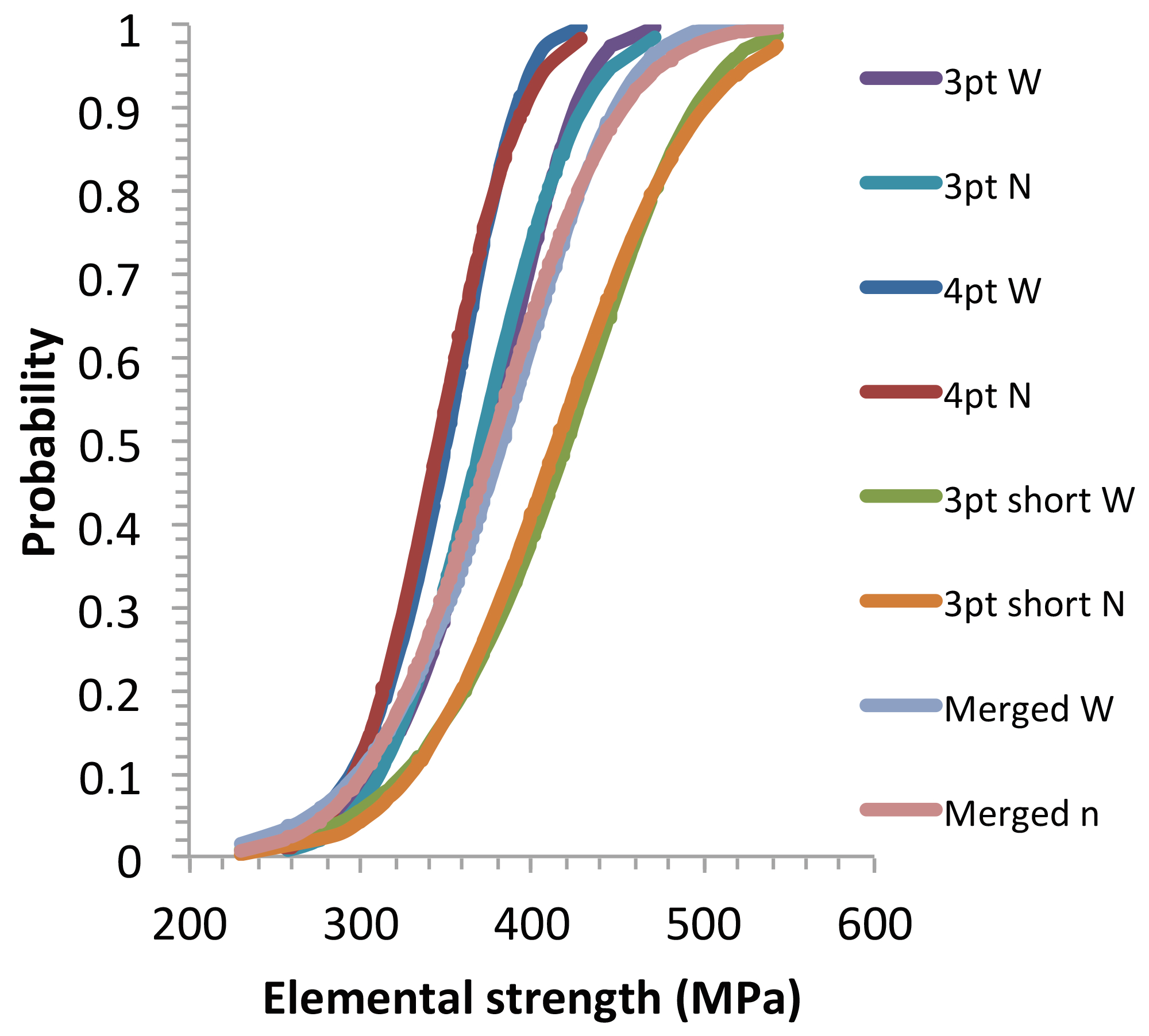
The normal flaw strength CDFs were calculated using Equation (7), and the Weibull CDFs were calculated using Equation (13) for the parameters given in Table 3. Figure 3 shows the excellent agreement of Weibull distributions with the normal reference ones. The values of the correlation coefficients given in Table 2 highlight a good agreement, which indicates that the distributions of the flaw strengths can be described using Weibull functions.

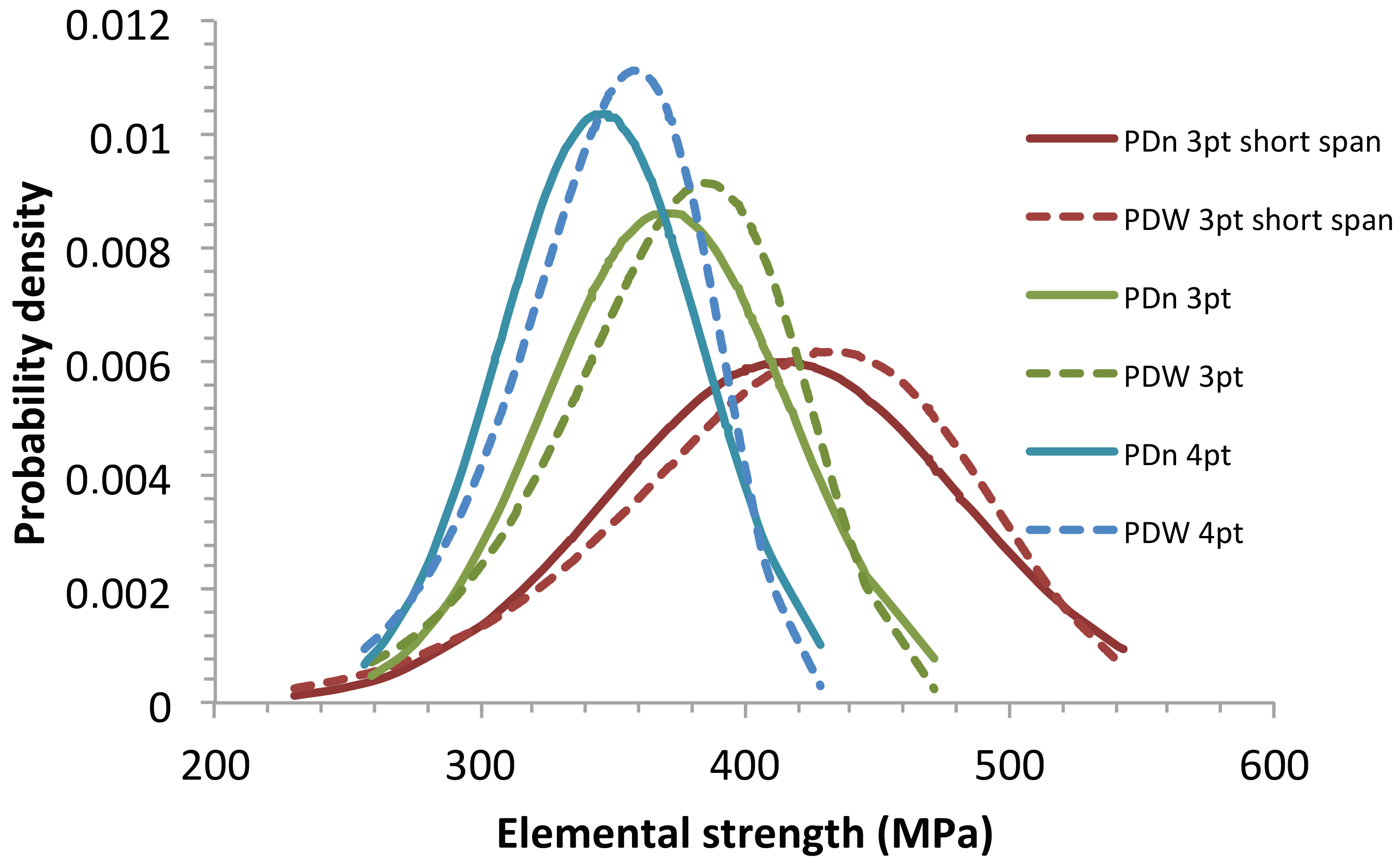
The discrepancies between the Gauss and Weibull probability density functions (PDFs) can be noted in Figure 4. These curves amplify the subtle differences between the normal and Weibull cumulative distributions that did not appear distinctly on Figure 3. This result moderates the above conclusion concerning correlation between the normal and Weibull functions for the flaw strengths. Therefore, it can be considered that the Weibull distribution may be regarded only as an acceptable approximation of a flaw strength distribution.

The PDFs show the same trends as above regarding the dependence of flaw strengths on the loading mode and the effective volume size. The peak probability density increased with the effective volume size, whereas the flaw strength interval decreased towards the same low strength extreme (Table 1). Like the p-quantile diagrams, this trend describes the shrinkage of the flaw strength interval.

3.3. Predictions of CDFs

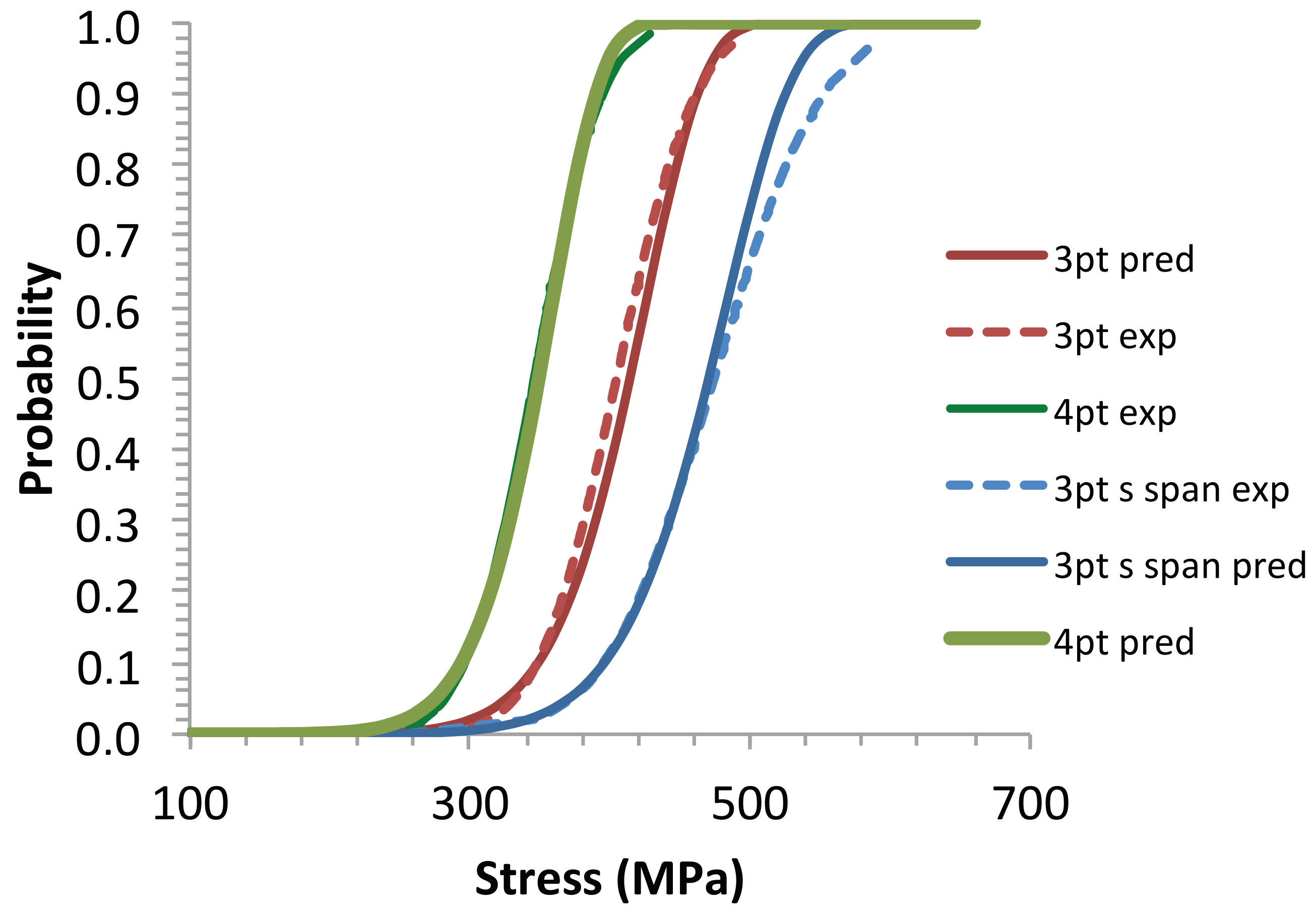
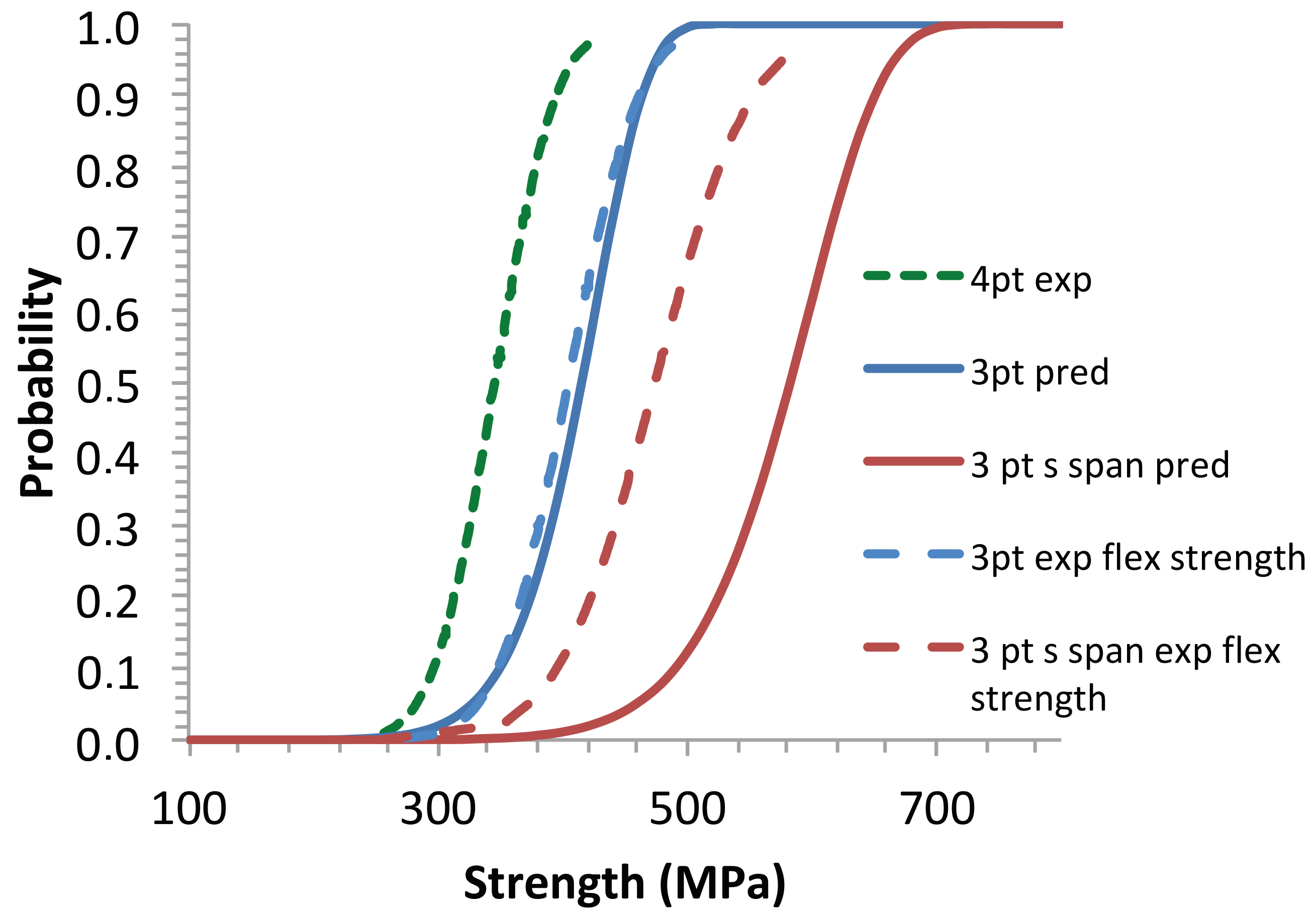
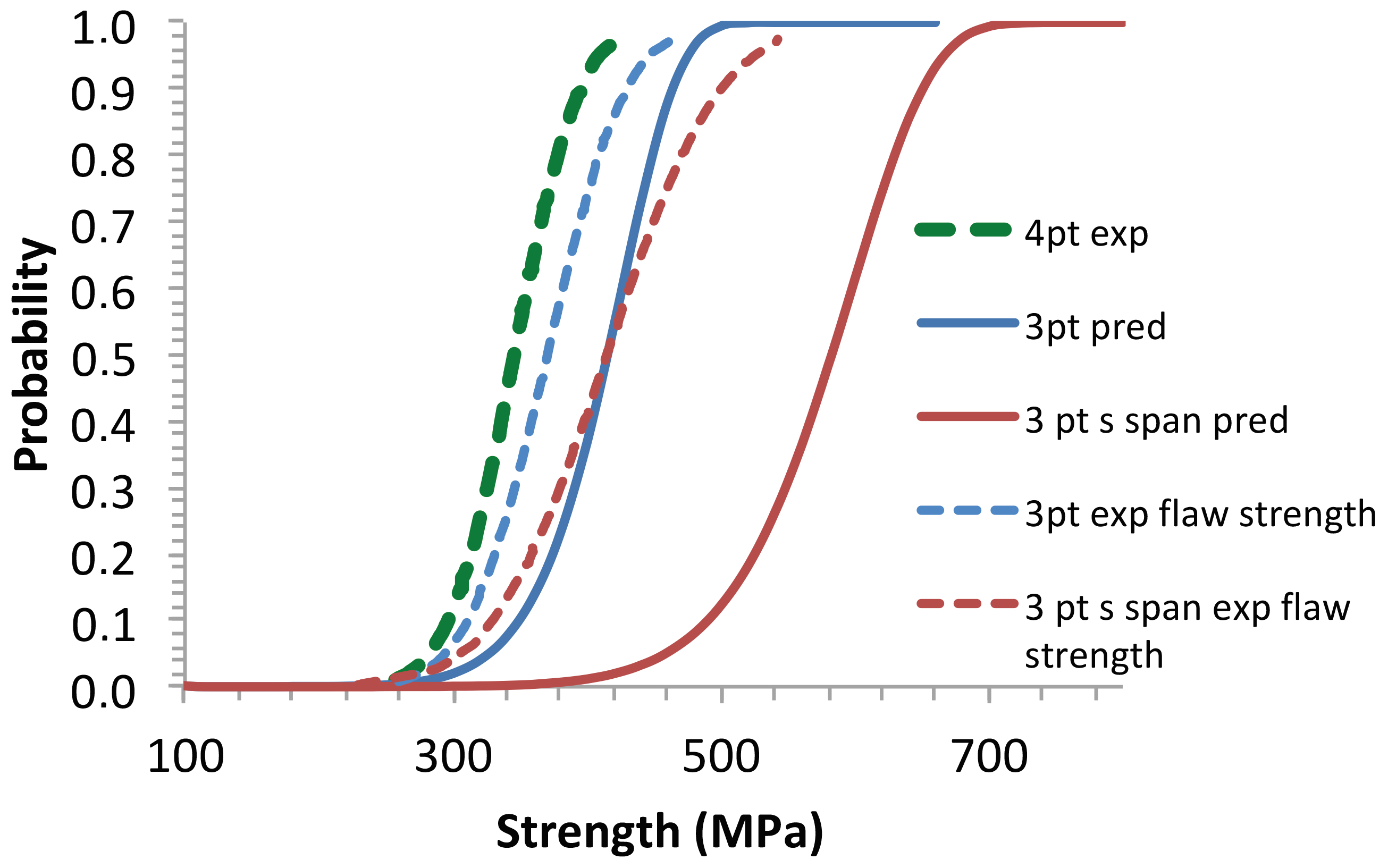
The failure probabilities were calculated using Equations (9) and (15) and the statistical parameters derived from the 4pt-bending tests given in Table 3. The predicted CDFs were compared with the reference distributions of the flexural (Figure 5 and Figure 6) and flaw strengths (Figure 7). The 4pt bending CDF was well fitted according to the elemental strength model for the parameters λ and S₀ given in Table 3 and for I(λ, 0, 0) = 0.25 [2] (Figure 4). The 3pt bending CDFs were satisfactorily predicted by the elemental strength model for these latter values of λ, S₀, and I(λ, 0, 0) (Figure 4). Figure 5 shows satisfactory Weibull predictions of CDF for the 3-point bending strengths (long span) from the 4-point bending parameters. By contrast, the Weibull model underestimated the failure probabilities for the short span flexural strengths (Figure 5) and did not properly describe the evolution of flaw strengths when the effective volume decreased (Figure 6).

4. Discussion: Implications

4.1. Merged Flaw Strength Distribution

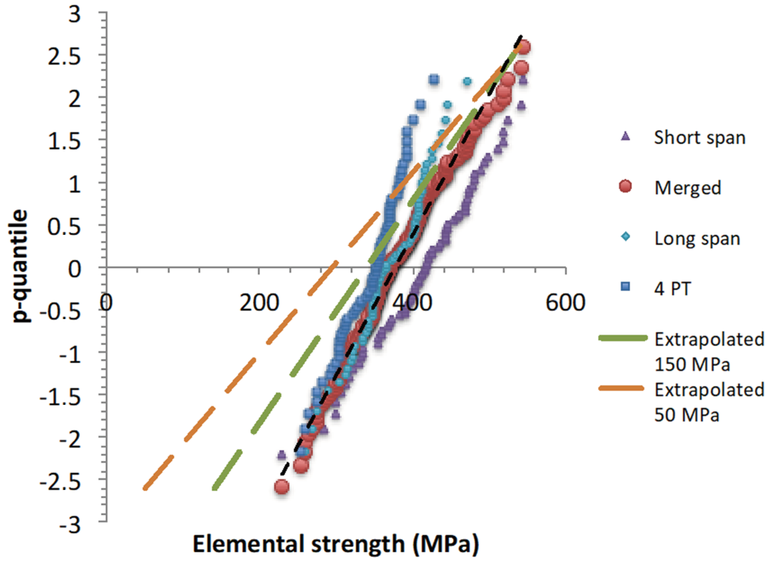
The elemental strengths are independent of volume size, being the strengths of flaws. Therefore, the three flaw strength datasets were merged. The outcome gives a linear p-quantile diagram (Figure 8) with a high correlation coefficient (Table 2). The result indicates that the merged diagram also follows a single normal distribution function, and thus that all the flaws belong to the same family (Figure 7). This allows us to infer that the populations of flaw strengths in the test specimens are subsets of a wider set of data. The merged population may characterize the whole population for the batches of the test specimens of the present paper, as suggested by the same value for the lowest flaw strengths. However, it may not include more severe flaws that were not activated, owing to the stress state that activates unequally the flaws.

The statistical parameters are given in Table 3. They are close to the parameters of the flaw strength distribution derived from the short span 3-point bending tests.

4.2. Extrapolated Flaw Strength Distribution

The comparison of the flaw strengths on PDFs, or p-quantile diagrams, indicates that the underlying flaw populations displayed variation. Thus, they cannot be regarded as being representative of the material type. On the basis of the above results, it seems logical to think that the flaw strength distributions obtained on various batches of specimens belong to a unique distribution which is characteristic of the whole flaw population existing in the material at a larger volume size. The existence of a material characteristic flaw strength distribution was evidenced using fiber tows [28]. Thus, it was shown that there exists a critical tow size above which the flaw strength distribution is invariant. Therefore, an attempt was made to construct a flaw strength distribution that would be representative of the SiC ceramic assessed in the present paper. This population would be obtained on a larger volume such that the underlying flaw population includes flaws which are weaker than those characterized on the bending specimens and which are present in the original plates. The extrapolation to distributions including weaker flaws was carried out using the p-quantile diagrams.

A linear p-quantile diagram is symmetrical to the mean strength per construction since z_pmax and z_pmin are symmetrical to z_p = 0. These remarkable features enable the construction of extrapolated p-quantile diagrams with broader flaw strength distributions.

z_pmax and z_pmin depend on the number of data through according to the following equations:

$$z_{pmax}={\mathsf{\Phi }}^{-1}\left(\frac{n}{n+1}\right)$$

(20)

$$z_{pmin}={\mathsf{\Phi }}^{-1}\left(\frac{1}{n+1}\right)$$

(21)

The slope of the p-quantile diagram is

$$\frac{z_{pmax-}{z}_{pmin}}{S_{max}-S_{min}}=\frac{1}{s}$$

(22)

The predictions of p-quantile diagrams and CDFs for a specified value of S_min were carried out as follows: The value of n is selected first. Then, z_pmax and z_pmin are calculated using Equations (20) and (21). Then, the values of S_min and S_max allow the definition of the p-quantile straight line. The value of μ corresponds to z_p = 0, and the standard deviation is derived from the slope (=1/s) (Equation (22)). From μ and s, one can derive the Weibull parameters m and S_s (Equations (18) and (19)).

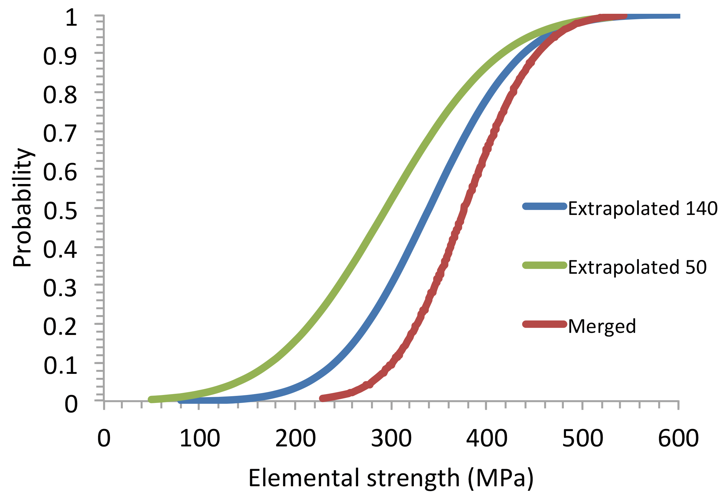
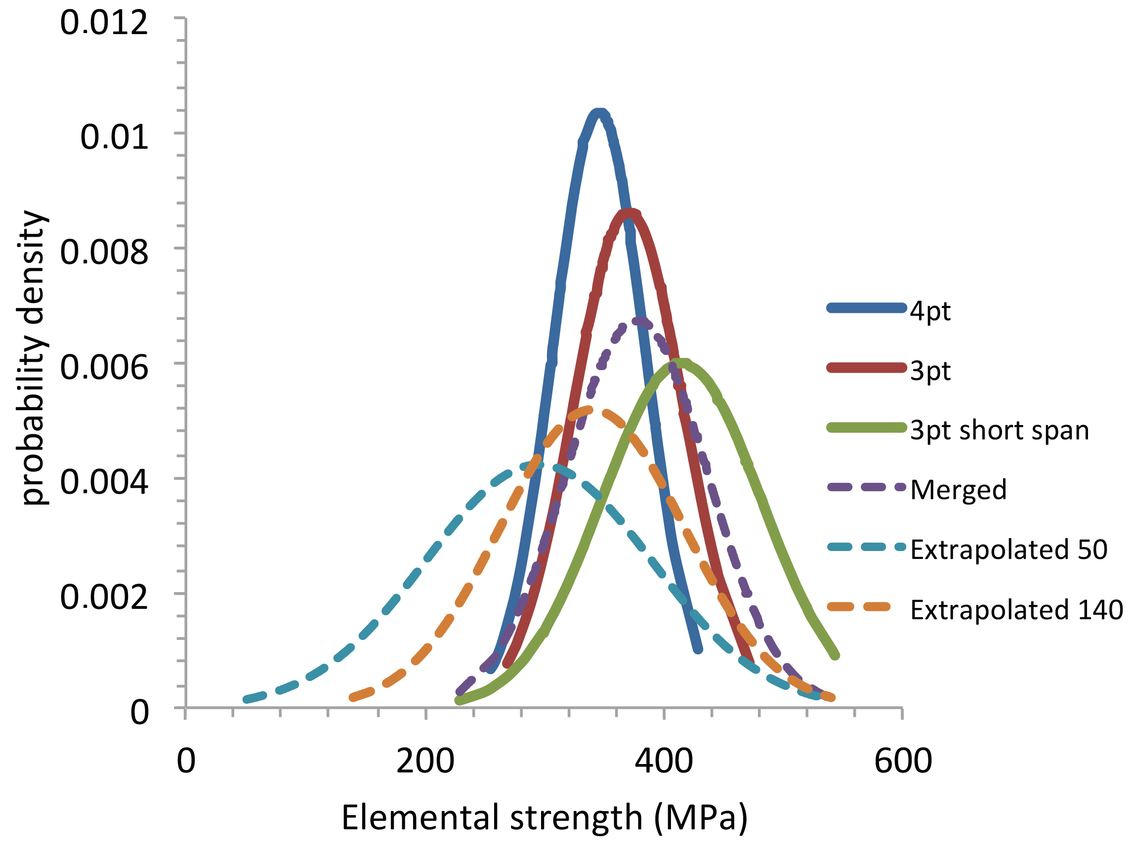
Figure 8 shows the extrapolated p-quantile diagrams for z_pmax = −z_pmin = 2.6, n = 210, S_min = 50 and 140 MPa, and S_max = 540 MPa. Figure 9 and Figure 10 show the corresponding normal CDFs and PDFs. These CDFs provide the probability of existence of flaw strength in a piece of material containing flaws having strengths larger than 50 or 140 MPa. S_min = 140 MPa is the strength of a 1 mm flaw, and S_min = 50 MPa is the strength of an 8 mm flaw when K_IC= 5 MPa√m. The 8 mm size is quite large with respect to the thickness of the initial plates. However, it may be considered a conservative limit. The value of the low strength extreme can be refined using non-destructive testing methods to detect and eliminate those specimens with flaws larger than a given value. S_max was taken as the high strength extreme of the merged distribution.

Such a representative function would be useful for material comparison purposes. It also allows the anticipation of the appropriate flaw strength distribution for the prediction of strength at large volumes. If the critical volume size existed above that in which the piece contains the whole population of flaws, there would not be size effect above the critical volume size. Below the critical volume size, the representative distribution of flaw strengths depends on the reproducibility of the flaw strength distribution.

4.3. Influence of n and Size

The p-quantile diagrams depend on the following parameters: the boundaries of the z_p interval determined by n the number of strength data and the boundaries of the elemental strength interval. These values define the p-quantile diagram, the normal statistical parameters s and μ, and the Weibull parameters.

In a uniform tensile stress state, the increase in the volume size may be regarded as equivalent to an increase in the number of flaw strength data n. In the presence of a stress gradient, this trend may be affected, as weak flaws may not be activated due to their location with respect to stress magnitude, whereas stronger flaws may be activated instead. A larger number of bending specimens is thus required to increase the chance that a broader spectrum of flaws is activated.

4.3.1. Influence of n on p-Quantile Maximum Values

The influence of n on z_pmax = −z_pmin was calculated using Equation (20). Figure 11 indicates that z_pmax increases slowly with n, for n > 200. But, there is no limit.

4.3.2. Influence of n and Volume on Statistical Parameters

From Equation (22) of the slope of the p-quantile diagram, the standard deviation can be obtained using the following:

$$s=\frac{S_{max}-\mu }{z_{pmax}}=\frac{S_{max}-\mu }{{\mathsf{\Phi }}^{-1}\left(\frac{n}{n+1}\right)}$$

(23)

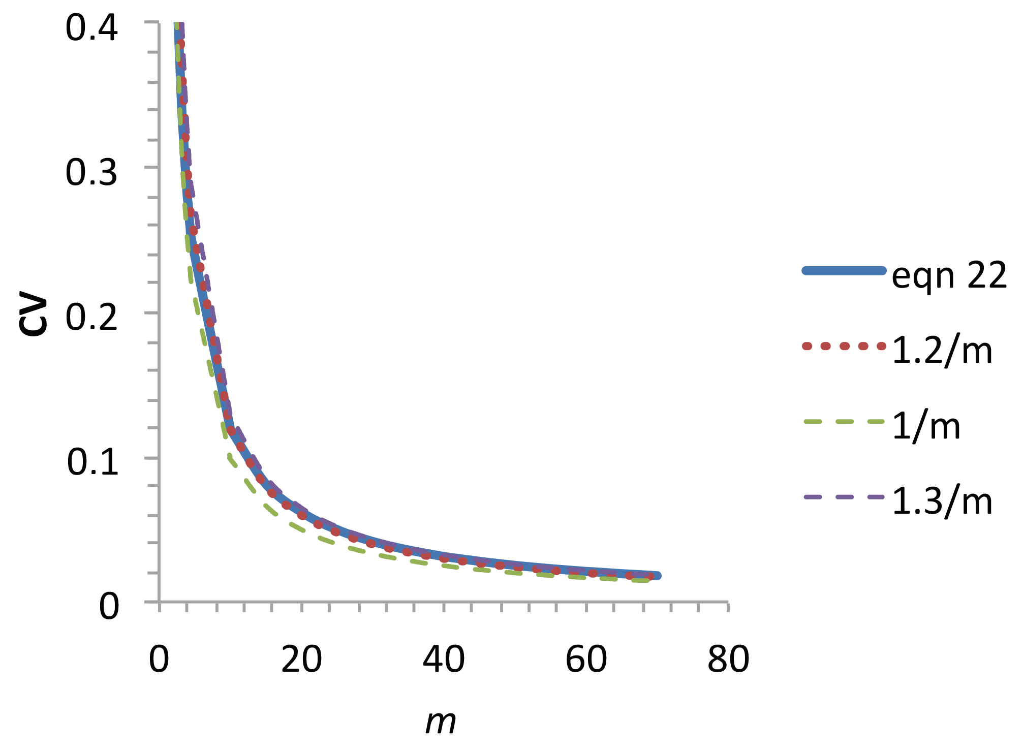
Figure 12 shows that Equation (24) is a good approximation of the coefficient of variation (CV = μ/s; Equation (18)) for the range of m values observed on ceramics. It is not significantly affected by a small variation in the constant around 1.2.

$$CV=\frac{1.2}{m}$$

(24)

Trends in the statistical parameter variation with the value of n or of the volume size were determined using Equations (23) and (24). The main results are reported in

Table 5. Main trends in the influence of n and V changes on the Weibull modulus.

n, V	Smin	Smax	Mean μ	Slope 1/s	s	m
n↗ V = cst	constant	constant	constant	↗	↘	↗
n↗ V = cst	constant	↗	↗	↗	↘	↗
n = cst V↗	constant	↘	↘	↗	↘	indeterminate
V↗ n↘	constant	↘	↘	↘	↗	↘
V ↗	↘	↘	↘	↗	↘	indeterminate
V ↗	↘	↘	↘	↘	↗	↘

.

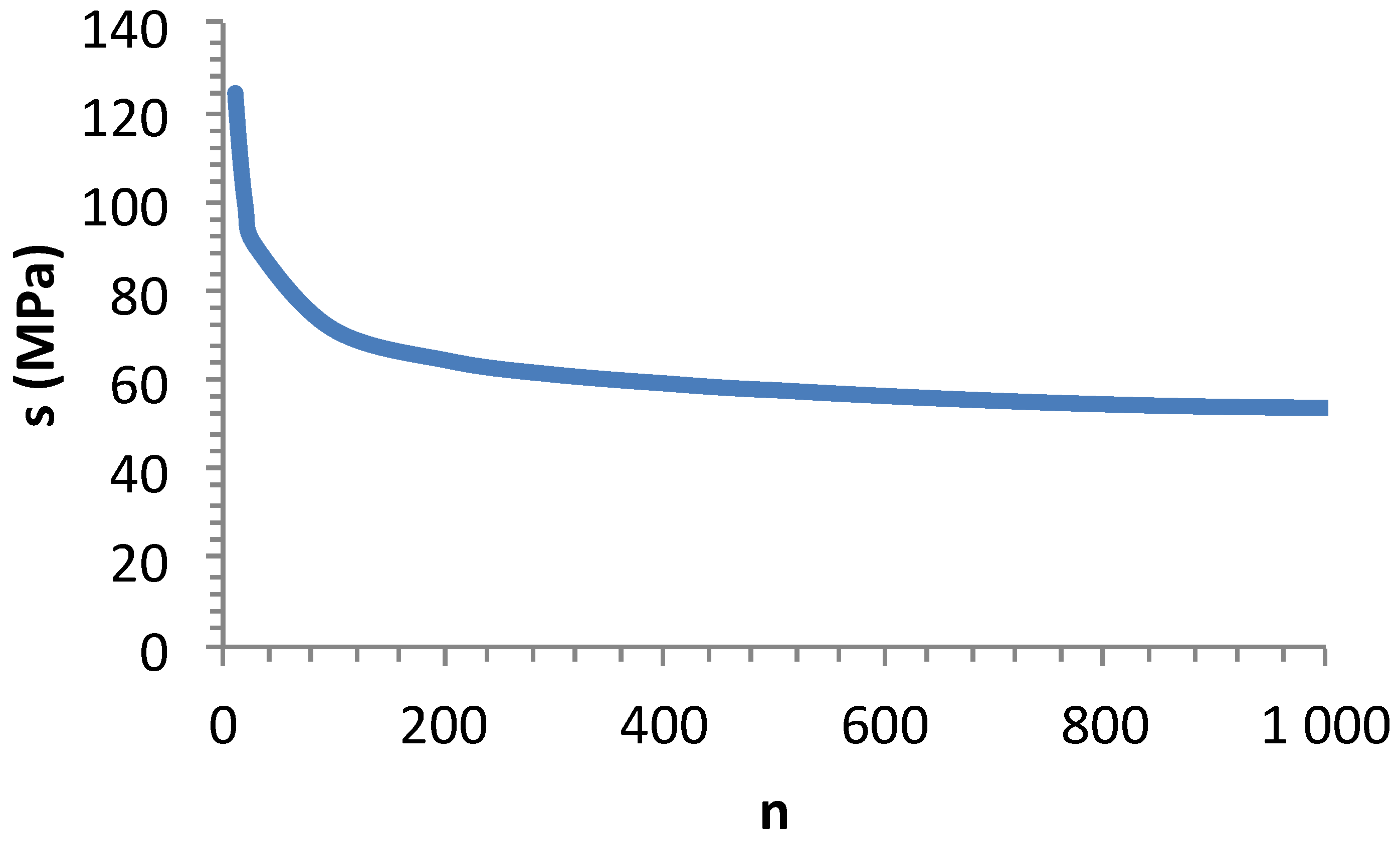
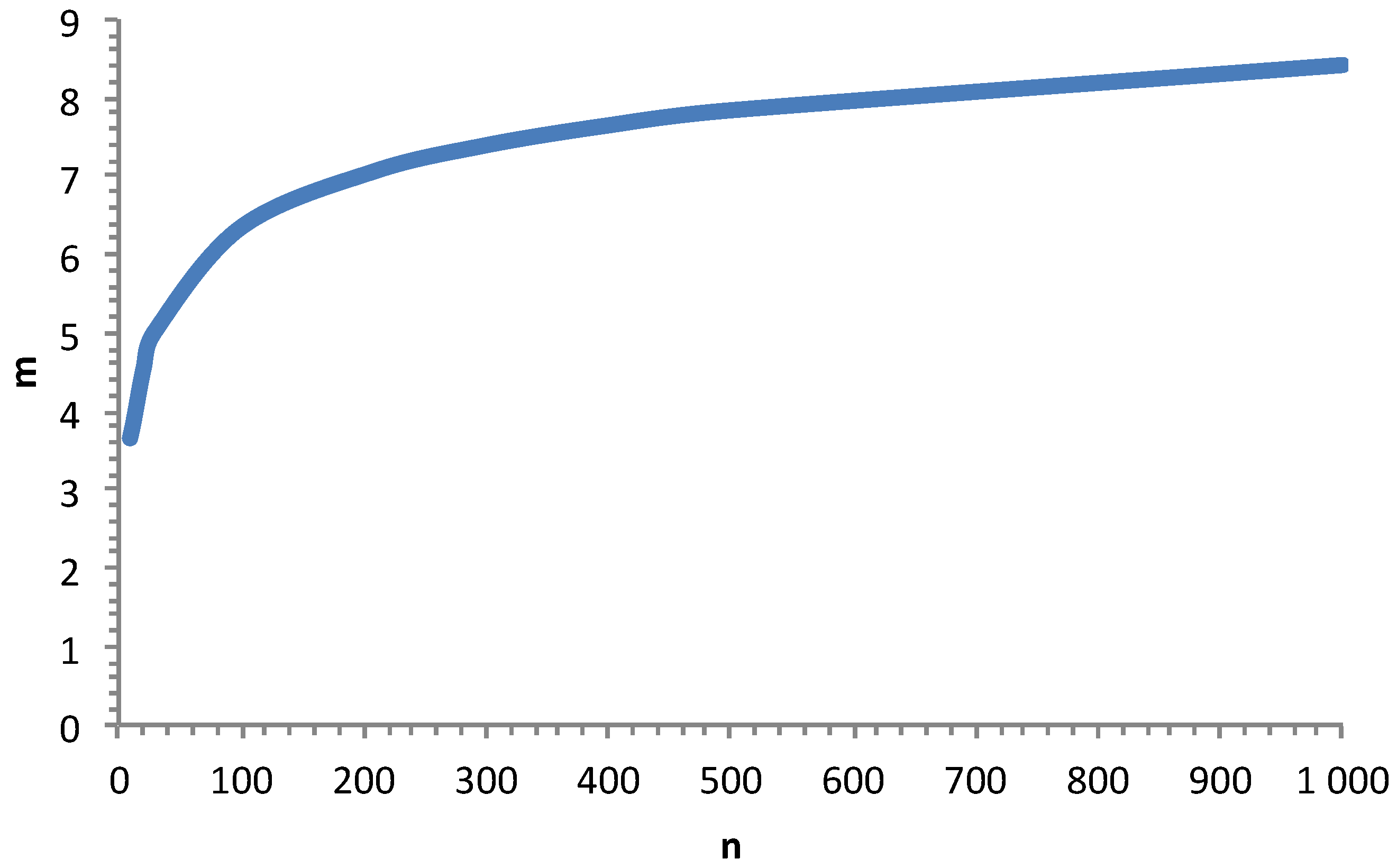
When the flaw strength interval and μ are constant, s is a decreasing function of increasing n (Figure 13). As a consequence, the Weibull modulus increases with n, as shown in Figure 14. It appears that there is no maximum value for m. Thus, it may be difficult to identify an appropriate estimate of m. For the purpose of the comparison of different distributions, it is thus necessary to consider batches of identical numbers of specimens.

When the flaw strength interval is constant and shifted towards lower values, μ decreases and s is a decreasing function as the slope increases with n. The trend in the Weibull modulus variation is indeterminate on the basis of Equation (24) (Table 5). m may increase, decrease, or remain constant. It remains constant only if μ and s remain proportional. If n is constant, the slope and s are constant so that m decreases according to Equation (24). This latter case was not reported in Table 5.

When the flaw strength interval is changed and shifted to lower values, μ decreases and s may increase or decrease with increasing n. m decreases with an increase in s. Then, its variation is indeterminate when s decreases (Table 5). As before, it remains constant only if μ and s remain proportional.

Both latter cases can be encountered at constant or increasing volumes. Thus, it appears that m does not take a unique value. It depends on the variability of the underlying flaw strength population in the test specimens from batch to batch, characterized by the variation in the standard deviation (Table 5). m invariant requires that μ and s are proportional according to Equations (18) and (24). It can be anticipated that this requirement implies a reproducible spatial distribution of the flaws.

These results are consistent with many papers that reported a big variation in m estimates from various laboratories testing different batches of specimens. Obviously, this is an issue for the prediction of the volume dependence of the strength. For this reason, the determination of a characteristic flaw strength distribution, as proposed in this paper, is an interesting alternative that provides the probability of the presence of flaws in the material and not only in small specimens. It can be used for purposes of comparing materials or components when those components with flaws larger than a given value have been eliminated. Furthermore, failure predictions on the components can be performed with the appropriate parameters instead of the parameters estimated on small specimens that may display significant variability.

4.4. Validity of the Uniaxial Analysis for a Short Span

In a previous paper [29], it was shown that the shear components can be reasonably neglected when d/l = 0.4. Local perturbations can arise on short span specimens in the vicinity of supports and loading point. It was found that the equation of the elementary beam theory provides a satisfactory value of strength [24]. The possible effect of the loading points is not detrimental since it concerns local compressive stresses. The fractography of the broken specimens clearly showed that failure occurred from the tensile part of the specimens. Furthermore, the plane of the fracture origin was always perpendicular to the longitudinal stress. This suggests that the elemental strength was parallel to the longitudinal stress. This supports the validity of the uniaxial elemental strength model for the short span specimens of this paper.

5. Conclusions

The p-quantile diagrams showed that the flaw strength data followed normal distributions in different non-uniform stress states, as well as when they were merged into a single set. The flexural strengths also showed normal distribution.

The strength data also followed Weibull distribution functions. Maximum likelihood and moment methods provided very close estimates of Weibull distribution parameters.

The fit of Weibull distributions to normal distributions was acceptable.

The elemental strength model permitted satisfactory predictions of flexural strength distributions from the flaw strength distribution of the 4-point bending specimens.

Weibull predictions from 4pt bending strength distributions overestimated the 3pt bending flaw strength distributions and the short-span flexural strength distributions.

The strength distribution may characterize only the batch of test specimens used for the determination of strength data. The distribution of critical flaw strengths may vary from batch to batch. The population of critical flaws is characterized by the size given by the number of flaw strength data (n), the weakness given by the strength interval (S_min, S_max), the mean strength (μ), the dispersion given by the standard deviation (s), and the reproducibility given by the CV. The Weibull modulus variability results from the variation in these parameters. It remains constant when n or V increase only if μ and s remain proportional (constant CV).

The extrapolation of experimental p-quantile diagrams through including weaker flaw strengths is an alternative approach to size effects based on the probability of existence of critical flaw strengths. It also allows anticipating flaw strength distributions in larger specimens for failure predictions using the elemental strength model.

The critical specimen size for which the flaw strength population is representative of the total critical flaw population inherent to the material type can be approached using both p-quantile diagrams and a technique detecting the most deleterious flaws.

References

1. Weibull, W. A statistical distribution function of wide applicability. J. Appl. Mech. 1951, 18, 293–297. [Google Scholar] [CrossRef]
2. Lamon, J. Brittle Fracture and Damage of Brittle Materials and Composites: Statistical-Probabilistic Approaches; ISTE Press–Elsevier: London, UK, 2017; ISBN 9781785481215. [Google Scholar]
3. Gong, J. A new probability index for estimating Weibull modulus for ceramics with least square method. J. Mater. Sci. Lett. 2000, 19, 827–829. [Google Scholar] [CrossRef]
4. Barnett, V. Probability plotting methods and order statistics. J. R. Stat. Soc. 1975, C24, 95–108. [Google Scholar] [CrossRef]
5. Watson, A.S.; Smith, R.L. An examination of statistical theories for fibrous materials in the light of experimental data. J. Mater. Sci. 1985, 20, 3260–3270. [Google Scholar] [CrossRef]
6. Paramonov, Y.; Andersons, J. A family of weakest link models for fiber strength distribution. Compos. Part A 2007, 38, 1227–1233. [Google Scholar] [CrossRef]
7. Phani, K.K. A new modified Weibull distribution function for the evaluation of the strength of silicon carbide and alumina fibres. J. Mater. Sci. 1988, 23, 2424–2428. [Google Scholar] [CrossRef]
8. Amaniampong, G.; Burgoyne, C.J. Statistical variability in the strength and failure strain of aramid and polyester yarns. J. Mater. Sci. 1994, 29, 5141–5152. [Google Scholar] [CrossRef]
9. Bergman, B. On the estimation of the Weibull modulus. J. Mater. Sci. Lett. 1984, 3, 689–692. [Google Scholar] [CrossRef]
10. Sullivan, J.D.; Lauzon, P.H. Experimental probability estimators for Weibull plots. J. Mater. Sci. Lett. 1986, 5, 1245–1247. [Google Scholar] [CrossRef]
11. Basu, B.; Tiwari, D.; Kundu, D.; Prasad, R. Is Weibull Distribution the Most Appropriate Statistical Strength Distribution for Brittle Materials? Ceram. Int. 2009, 35, 237–246. [Google Scholar] [CrossRef]
12. Lu, C.; Danzer, R.; Fischer, F.D. Fracture statistics of brittle materials: Weibull or normal distribution. Phys. Rev. E 2002, 65, 06702. [Google Scholar] [CrossRef] [PubMed]
13. Peirce, F.T. Tensile Tests for Cotton Yarns—The Weakest Link. J. Text. Inst. 1926, 17, 355–368. [Google Scholar]
14. Epstein, B. Application of the theory of extreme values in fracture problems. J. Am. Statist. Assoc. 1948, 43, 403–412. [Google Scholar] [CrossRef]
15. R’Mili, M.; Godin, N.; Lamon, J. Flaw strength distributions and statistical parameters for ceramic fibres: The Normal distribution. Phys. Rev. E 2012, 85, 1106–1112. [Google Scholar]
16. Lamon, J.; R’Mili, M. Investigation of flaw strength distributions from tensile force-strain curves of fiber tows. Compos. Part A 2021, 145, 106262. [Google Scholar] [CrossRef]
17. Lissart, N.; Lamon, J. Statistical analysis of failure of SiC fibers in the presence of bimodal flaw populations. J. Mater. Sci. 1997, 32, 6107–6117. [Google Scholar] [CrossRef]
18. Vu, C.-C.; Tran, H.-H. Performance analysis of methods to estimate Weibull parameters for the compressive strength of concrete. Case Stud. Constr. Mater. 2023, 19, e02330. [Google Scholar] [CrossRef]
19. Freudenthal, A. Statistical Approach to Brittle Fracture. Chapter 6. In Fracture; Liebowitz, H., Ed.; Academic Press: New York, NY, USA, 1968; Volume II. [Google Scholar]
20. Gumbel, E. Statistics of Extremes; Columbia University Press: New York, NY, USA, 1968. [Google Scholar]
21. Jayatilaka, A.D.S.; Trustrum, K. Statistical approach to brittle fracture. J. Mater. Sci. 1977, 10, 1426–1430. [Google Scholar] [CrossRef]
22. Argon, A.S.; McClintock, F.A. Mechanical Behavior of Materials; Addison-Wesley: Reading, MA, USA, 1966. [Google Scholar]
23. Batdorf, S.B.; Crose, J.G. A statistical theory for the fracture of brittle structures subjected to nonuniform polyaxial stresses. J. Appl. Mech. 1974, 41, 459–464. [Google Scholar] [CrossRef]
24. Lamon, J. Ceramics reliability: Statistical analysis of multiaxial failure using the Weibull approach and the Multiaxial Elemental Strengh model. J. Am. Ceram. Soc. 1990, 73, 2204–2212. [Google Scholar] [CrossRef]
25. Lamon, J.; Evans, A.G. The statistical analysis of bending strengths for brittle solids: A multiaxial fracture problem. J. Am. Ceram. Soc. 1983, 66, 177–182. [Google Scholar] [CrossRef]
26. Bhattacharya, P.; Bhattacharjee, R. A study on Weibull distribution for estimating the parameters. J. Appl. Quant. Methods 2010, 5, 234–241. [Google Scholar] [CrossRef]
27. Bin Deng, B.; Wang, X.; Jiang, D.; Gong, J. Description of the statistical variations of the measured strength for brittle ceramics: A comparison between two-parameter Weibull distribution and normal distribution. Process. Appl. Ceram. 2020, 14, 293–302. [Google Scholar] [CrossRef]
28. Lamon, J.; R’Mili, M. Investigation of Specimen Size Effects on P-Quantile Diagrams and Normal Distributions of Critical Flaw Strengths in Fiber Tows. J. Compos. Sci. 2022, 6, 171. [Google Scholar] [CrossRef]
29. Lamon, J. Statistical analysis of fracture of Silicon Nitride using the short span bending technique. Int. J. Turbo Jet Engines 1988, 5, 13–22. [Google Scholar] [CrossRef]
Figure 1. Pores in the fracture surface of a silicon carbide specimen. The scale bar indicates 10 μm.
Ceramics 07 00050 g001
Figure 2. p-quantile diagrams obtained for the sets of strength data obtained on the bending tests. The solid lines indicate the regression lines.
Ceramics 07 00050 g002
Figure 3. Comparison of Weibull (referred to as W) and normal (referred to as N) cumulative distribution functions for the elemental strengths.
Ceramics 07 00050 g003
Figure 4. Comparison of the Weibull (PDW) and Gauss (PDn) probability density functions.
Ceramics 07 00050 g004
Figure 5. Size effects: predictions of the flexural strengths using the multiaxial elemental strength model equation for the flaw strength parameters derived from the 4pt bending tests. Comparison with the experimental flexural strength distributions.
Ceramics 07 00050 g005
Figure 6. Size effects: predictions of the flexural strengths using the Weibull model equation for the statistical parameters derived from the 4pt bending tests. Comparison with the experimental flexural strength distributions.
Ceramics 07 00050 g006
Figure 7. Size effects: predictions of the flaw strengths using the Weibull model for the flaw strength parameters derived from 4pt bending tests. Comparison with the experimental flaw strength distributions.
Ceramics 07 00050 g007
Figure 8. Merged and extrapolated p-quantile–flaw strength diagrams. Comparison with those obtained from the 3-point and 4-point bending tests.
Ceramics 07 00050 g008
Figure 9. Normal CDFs derived from the merged and extrapolated p-quantile–flaw strength diagrams.
Ceramics 07 00050 g009
Figure 10. Gaussian PDFs derived from the merged and extrapolated p-quantile–flaw strength diagrams.
Ceramics 07 00050 g010
Figure 11. Influence of the number of flaw strength data n on the extreme values zpmax (=−zpmin).
Ceramics 07 00050 g011
Figure 12. Variation in the coefficient of variation (Equation (18)) with m. Comparison with functions 1/m, 1.2/m, and 1.3/m.
Ceramics 07 00050 g012
Figure 13. Influence on n on standard deviation when the flaw strength interval and μ are constant.
Ceramics 07 00050 g013
Figure 14. Influence of n on m when the strength interval and the mean strength are kept constant.
Ceramics 07 00050 g014