Article

Detecting Anomalous Non-Cooperative Satellites Based on Satellite Tracking Data and Bi-Minimal GRU with Attention Mechanisms

National Key Laboratory of Information Systems Engineering, National University of Defense Technology, Changsha 410003, China
*
Author to whom correspondence should be addressed.
Appl. Syst. Innov. 2025, 8(6), 163; https://doi.org/10.3390/asi8060163
Submission received: 25 September 2025 / Revised: 18 October 2025 / Accepted: 22 October 2025 / Published: 27 October 2025
(This article belongs to the Section Control and Systems Engineering)

Abstract

In recent years, the number of satellites in space has experienced explosive growth, and the number of non-cooperative satellites requiring close attention and precise tracking has also increased rapidly. Despite this, the world’s satellite precision tracking equipment is constrained by factors such as a slower growth in numbers and a scarcity of available deployment sites. To rapidly and efficiently identify satellites with potential new anomalies among the large number of cataloged non-cooperative satellites currently transiting, we have constructed a Bi-Directional Minimal GRU deep learning network model incorporating an attention mechanism based on Minimal GRU. This model is termed the Attention-based Bi-Directional Minimal GRU model (ABMGRU). This model utilizes tracking data from relatively inexpensive satellite observation equipment such as phased array radars, along with catalog information for non-cooperative satellites. It rapidly detects anomalies in target satellites during the initial phase of their passes, providing decision support for the subsequent deployment, scheduling, and allocation of precision satellite tracking equipment. The satellite tracking observation data used to support model training is predicted through Satellite Tool Kit simulation based on existing catalog information of non-cooperative satellites, encompassing both anomaly free data and various types of data containing anomalies. Due to limitations imposed by relatively inexpensive observation equipment, satellite tracking data is restricted to the following categories: time, azimuth, elevation, distance, and Doppler shift, while incorporating realistic noise levels. Since subsequent precision tracking requires utilizing more satellite pass time, the duration of tracking data collected during this phase should not be excessively long. The tracking observation time in this study is limited to 1000 s. To enhance the efficiency and effectiveness of satellite anomaly detection, we have developed an Attention-based Bi-Directional Minimal GRU deep learning network model. Experimental results demonstrate that the proposed method can detect non-cooperative anomalous satellites more effectively and efficiently than existing lightweight intelligent algorithms, outperforming them in both completion efficiency and detection performance. It exhibits superiority across various non-cooperative satellite anomaly detection scenarios.

1. Introduction

Space security [1] represents a new frontier in national security, and safeguarding it is crucial for ensuring the integrity of a nation’s strategic security interests. Detecting potential anomalies in non-cooperative satellites is one of the core capabilities of modern space situational awareness [2,3,4], holding critical and multifaceted significance and utility for maintaining space security [5]. With the continuous advancement of space technology, humanity’s exploration of outer space has intensified rapidly. The number of artificial satellites in space has grown exponentially, and the security situation in space has become increasingly severe. An increasing number of countries are participating in space exploration, leading to growing congestion in space with tens of thousands of active satellites [6,7,8]. At the same time, high-precision observation resources such as large-aperture optical telescopes are limited in number, prohibitively expensive, and require substantial operational and maintenance costs. This makes it challenging to conduct precise tracking and observation of all transiting non-cooperative satellites, posing significant difficulties for hazard warnings and threat assessments [9,10]. The fundamental approach to resolving the current contradiction between the infinite nature of observational demands and the finite availability of observational resources lies in the scheduling and allocation of satellite observation resources [11]. In addition to high-precision satellite observation equipment, the world contains numerous satellite observation devices that are less sophisticated but exist in greater numbers. These include optical telescopes, low-cost phased-array radars, or mechanically scanned radars. While the satellite tracking data they collect has limited accuracy, fewer data categories, and lower resolution, they offer advantages such as low cost, broad coverage, distributed deployment, and continuous operation. These devices generate massive, high-speed, and highly variable satellite observation data, leading to the gradual phasing out of traditional methods from modern satellite observation systems. To address this challenge, advanced data analysis techniques, particularly deep learning, have emerged, making modern satellite observation systems increasingly complex and dynamic [12]. This study focuses on utilizing low-performance observation resources to monitor cataloged non-cooperative satellite transits during their initial phases, detecting potential anomalies through acquired tracking observation data. This work can determine whether to activate or call upon high-performance observation resources during the mid-to-late stages of non-cooperative satellite transits, providing a basis for decision-making on prioritizing observations of anomalous satellites. It not only optimizes the scheduling and allocation of satellite tracking and observation resources during time-critical situations but also reduces wear and tear on high-performance equipment and lowers operational and maintenance costs during routine operations. Prior to the entry of non-cooperative satellites into the observable range, we simulate and predict a certain number of satellite tracking datasets with relatively realistic noise levels using their cataloging information and the Satellite Tool Kit (STK) [13]. These datasets include both normal and various abnormal scenarios, which are then used to train a pre-built Bi-Directional Minimal [14] GRU deep learning network model incorporating an attention mechanism. Then, during the brief period immediately after the satellite enters the observable range, based on the actual tracking data from relatively low-performance observation equipment, a rapid assessment is made to determine whether the satellite may exhibit anomalies. Satellites identified as potentially anomalous are placed on a priority monitoring list, with subsequent consideration given to whether to activate precision tracking equipment for observation. The specific main contributions are as follows:
(1)
We propose a method for detecting anomalies in cataloged non-cooperative satellites using low-cost satellite observation resources, thereby providing a decision-making basis for the scheduling and allocation of high-value and high-precision satellite observation resources during tracking and observation of non-cooperative satellites. This experiment accounts for limitations inherent in satellite tracking data from low-cost satellite observation resources, such as relatively high data noise and fewer data categories. To ensure sufficient observation time for subsequent precision tracking, we imposed constraints on the experimental scenario: shorter observation durations and the need for lightweight models. Based on the aforementioned conditions, this paper constructs a deep learning anomaly detection model for cataloged non-cooperative satellites. The objective is to rapidly determine whether anomalies exist during the initial phase when cataloged non-cooperative satellites enter the observable range.
(2)
We propose a Bi-Directional Minimal GRU deep learning network model incorporating an attention mechanism to detect anomalies in cataloged non-cooperative satellites. First, to significantly reduce the number of parameters and computational complexity without substantially compromising model expressiveness, we adopted the Minimal GRU model as the foundational architecture for the entire network framework. Next, to capture the full contextual information at each time step, we enhanced the Minimal GRU, creating the Bi-Directional Minimal GRU. Finally, to enable the model to autonomously learn weights across different time steps and enhance detection performance, we incorporated an attention mechanism into the Bi-Directional Minimal GRU, ultimately forming the Attention-based Bi-Directional Minimal GRU model. This model enables rapid and effective anomaly detection for cataloged non-cooperative satellites.
(3)
We designed simulation experiments and validated the model’s effectiveness by analyzing the simulation results. Through comparative experiments between our Attention-based Bi-Directional Minimal GRU deep learning model and other lightweight algorithms, we demonstrated that our designed algorithm outperforms others in terms of efficiency and performance.
This paper is structured as follows: Section 2 reviews the current state of research on processing methods for satellite tracking data and multivariate time series data. Section 3 constructs a Bi-Directional Minimal GRU deep learning network model by integrating attention mechanisms; Section 4 designs comparative experiments to validate the superiority of the Attention-based Bi-Directional Minimal GRU deep learning network model. Section 5 summarizes the main contributions and conclusions of the paper and outlines future research directions.

2. Literature Review

This study is closely related to the literature on data mining of satellite tracking observation data and algorithms for identifying features in multiple time series. We present a concise review below.

2.1. Satellite Observation Data

The structure and format of satellite observation data [15] acquired by current ground stations exhibit significant diversity. However, they typically contain certain core structures and common elements, including timestamps, satellite identifiers, ground station identifiers, telemetry data [16], and tracking data [17]. The definitions of various types of satellite observation data are shown in Table 1.
Artificial satellites currently in space include cooperative satellites and non-cooperative satellites [10]. Among the non-cooperative satellites are space debris, satellite weapons, satellites with undisclosed maneuvering plans, and fuel-depleted, non-functional satellites. Satellites with undisclosed operational [10] plans are prioritized cataloging targets, with their cataloging information updated periodically. The subject of anomaly detection in this paper is cataloged non-cooperative satellites. Since most telemetry data [16] requires communication and data transmission with the target satellite, such satellites’ observational data typically do not include telemetry data. In this experimental scenario, the ground observation stations are fixed, and data simulation and model training must be performed independently for each target satellite. Therefore, the satellite observation data we use does not include satellite identifiers, ground station identifiers, or telemetry data.
In summary, the satellite observation data in the experiment includes timestamps and satellite tracking data, comprising five categories in total: time, azimuth, elevation angle, distance, and Doppler shift. Detecting satellite anomalies based on satellite tracking data essentially involves data mining or feature extraction of the tracking data to determine whether the satellite is operating abnormally. Prior to the 21st century, satellite tracking data processing was primarily based on physical models and statistical methods. These approaches relied on precise initial parameters, exhibited limited capability in handling nonlinear problems, and involved high computational complexity. In the 2000s, machine learning began to be applied to processing satellite tracking data. Representative techniques included supervised learning and unsupervised learning, which were employed to address the practical challenges posed by the rapid increase in satellite numbers and the growing dimensionality of data. Since the 2010s, deep learning technology has gradually emerged. Its advantages in automatic feature extraction, high nonlinear modeling, end-to-end optimization, and large-scale data processing [18] make it highly suitable for data mining and feature recognition in satellite observation data. Satellite tracking data constitutes a type of multivariate time series, whose primary characteristics include Time dependence, Spatial dependence, Spectral characteristics, noise characteristics, Shape characteristics, and similarity features [19]. The definitions of its main features are shown in Table 2.
The task of detecting satellite anomalies based on tracking data essentially involves identifying or extracting these six primary characteristics from the satellite tracking data structure through various algorithms. Generally speaking, Time dependence and Spatial dependence are the most significant data characteristics, followed by spectral characteristics, while the remaining three types of features have a relatively minor impact.

2.2. Algorithms for Mining Multivariate Time Series Data

In early research, multivariate time series analysis primarily relied on classical statistical methods. In classical statistical methods, approaches primarily designed to extract and identify time-dependent characteristics in data include Autoregression (AR) [20], Moving Average (MA) [21], Auto-Regression and Moving Average (ARMA) [22], and Autoregressive Integrated Moving Average (ARIMA) [23]. These methods are all suitable for fitting time series without pronounced periodicity. Classic statistical methods for extracting and identifying spatial dependencies in data include Vector Autoregression (VAR) [24], Vector Autoregressive Moving Average (VARMA) [25], and Vector Autoregressive Integrated Moving Average (VARIMA) [26], which have played a significant role in multivariate time series analysis. The classical methods for spectral analysis of multivariate time series primarily include the Fourier transform [27] and the discrete Fourier transform.
Since the 21st century, machine learning algorithms have been progressively applied to the field of multivariable time series data mining, with representative algorithms including Back Propagation Neural Networks (BPnetwork) [28] and Least Squares Support Vector Machines (LSSVM) [29]. In recent years, with the advancement of deep neural network technology, deep learning methods have been increasingly applied to time series data mining. Compared to classical statistical methods and traditional machine learning algorithms, deep learning offers several distinct advantages in time series data mining, including robust nonlinear modeling capabilities, adaptive learning, end-to-end learning capabilities, and the ability to process large-scale data. These advantages make deep learning a powerful tool for addressing time series-related problems, and it has gradually become one of the mainstream methods in the field of time series data mining [30]. Deep learning algorithms with strong data mining capabilities for multivariate time series include Recurrent Neural Networks (RNN) [31], Long Short-Term Memory networks (LSTM) [32], Gated Recurrent Unit (GRU) [33], Convolutional Neural Networks (CNN) [34], Attention Mechanisms [35], Transformer architecture [35], Graph Convolutional Networks (GCN) [36], and Graph Attention Networks (GAT) [37].
In practical applications, as new satellites continuously enter observable regions, anomaly detection for non-cooperative cataloged satellites and catalog information updates for anomalous non-cooperative satellites are conducted concurrently. Updating catalog information for anomalous non-cooperative satellites is one of the follow-up tasks that should be addressed after this research. This includes high-priority operations such as precise satellite orbit determination, which demands substantial server memory and computational resources. Therefore, the computational resources and memory allocated to this research must be limited. Furthermore, tens of thousands of satellites are currently operating in space, with numbers expected to grow significantly in the future. Often, we must simultaneously handle hundreds of non-cooperative cataloged satellites to build corresponding deep learning models for them. If the model structure is highly complex, with numerous parameters and high memory consumption, it not only consumes excessive time but also occupies too much server memory and computational resources. Therefore, we need to utilize lightweight models in our experiments whenever possible, ensuring their total parameters do not exceed 10 million while maintaining high training efficiency, strong detection performance, and low memory consumption. Traditional statistical algorithms generally perform worse than machine learning and deep learning algorithms. Additionally, they exhibit high feature engineering complexity, slow model training speeds, and high memory consumption. Therefore, we do not consider traditional statistical methods in this experimental scenario. Table 3 summarizes classical deep learning algorithms capable of handling multivariate time series, briefly describing their key principles while also outlining their primary advantages and defects.
Table 3 describes the principles and advantages and defects of each model solely in the context of handling time series data. Some common advantages and defects of algorithms have not been mentioned. For example, all deep learning algorithms suffer from poor interpretability. LSTM and GRU represent a comprehensive improvement over RNN in terms of performance. GAT also comprehensively outperforms GCN in terms of effectiveness and efficiency. Therefore, we exclude RNN and GCN from our comparative experiments. After a comprehensive comparison of the advantages and disadvantages of various models, we ultimately selected the GRU network model as the foundational architecture for the deep learning network used in satellite anomaly detection.

3. Problem Description and Modeling

This section first outlines an experimental scenario for detecting anomalies in cataloged non-cooperative satellites, followed by the integration of an attention mechanism to construct a Bi-Directional Minimal GRU deep learning network model tailored for this scenario.

3.1. Experiment Scenario Description

The experiment scenario described in this paper involves ground-to-air observation, specifically tracking and observing non-cooperative space targets using ground-based observation resources. This experiment scenario is divided into three phases: before cataloged non-cooperative satellites enter the observable region, the initial phase upon entering the observable region, and the mid-to-late phase. Prior to the entry of non-cooperative satellites into the observable region, simulations are conducted using existing satellite catalog information and STK software to generate both anomaly free satellite tracking observation data and various types of anomaly containing satellite tracking observation data. Based on simulation data, hundreds of Attention-based Bi-Directional Minimal GRU deep learning network models were trained for hundreds of non-cooperative satellites approaching the observable region. Each satellite corresponds to a specific model. Satellites and ground observation stations are both high-value assets. Authentic and relatively precise satellite tracking and observation data hold immense value and constitute classified information that is difficult to obtain. Therefore, this study primarily relies on simulated data, which represents a limitation of this research. STK utilizes precise physical models and algorithms [13] to generate high-accuracy simulation data, including information such as position, velocity, angular velocity, and attitude during satellite flight. STK has been validated by global professional institutions and NASA. Its simulation data features high precision, diverse types, strong real-time capabilities, excellent visualization, and robust scalability, resulting in highly authoritative outcomes. Satellite tracking data derived from existing catalog information and STK simulation predictions can effectively support model training. After model training is complete, during the initial phase when the satellite enters the observable region, actual tracking data is acquired using inexpensive ground-based satellite tracking observation equipment. Then, the data is fed into the model for analysis, identifying satellites that are highly likely to be anomalous from a large number of non-cooperative satellites. During the latter part of the satellite’s observable window, further consideration can be given to whether to allocate or deploy precision tracking equipment to observe non-cooperative satellites that have been confirmed to exhibit anomalies. The schematic diagram of the experimental scenario is shown in Figure 1.
When detecting satellite anomalies based on satellite tracking data, the anomalies primarily manifest as slight changes in the satellite’s orbit. If a satellite’s orbital changes are significant, it can be directly classified as an anomalous satellite without requiring any algorithm. Therefore, the satellite anomalies set in the simulation experiments are relatively minor and require assessment through models or algorithms. The sources of anomalies in non-cooperative satellites are multifaceted, including environmental impacts, sudden failures, or deliberate maneuvers. Regardless of the source of the anomaly, satellite anomalies identified based on satellite tracking data can be equated to the satellite having been subjected to abnormal forces. Therefore, the method employed in this experiment to simulate anomalous satellite orbital data involves applying a certain amount of anomalous dynamics to the satellite at a specific moment, while ensuring that the anomalous dynamics remain relatively small.
Although we need to handle hundreds or even thousands of satellites simultaneously within the entire experimental scenario, the construction and training of each individual model is tailored for a single satellite. The construction method and process for each satellite’s detection model are similar. In an experiment, the satellite mass was set to 100 kg, with a semi-major axis of 6,878,137 m, an eccentricity of 0.01, an orbital inclination of 0°, a ascending node right ascension of 0°, a near-apogee angle of 0°, and a true ascending node angle of 100 degrees. The ground observation station’s latitude was set to 39.9042 degrees, longitude to 116.4074 degrees, elevation to 43.5 m, and minimum observation elevation angle to 5 degrees. The tracking data recording interval was set to 10 s, with a total recording duration ranging from 800 to 1200 s. Other simulation parameters are set to their default values. When generating synthetic data samples, we add appropriate random noise and set 20% of the data to missing values. The impulse magnitude of all abnormal satellites is set to 2 newtons, with the type being pulse thrust and the duration lasting 1 s. One satellite anomaly dynamic time point is set every 200 s, totaling 10 points and ensuring that all satellite anomaly dynamics occur either before the satellite enters an observable region or within the time interval, during which satellite tracking data is recorded. A total of 1 normal scenario and 10 abnormal scenarios of satellite tracking observation data were simulated. For each category, 400 samples of satellite tracking data with varying noise levels were simulated, resulting in a total of 4400 samples.

3.2. Model Construction

After obtaining simulation data based on experimental scenarios, we construct anomaly detection models for cataloged non-cooperative satellites. We do this through first performing data preprocessing. Then, we explain the symbols used in the model’s principles. Finally, we construct the network model.

3.2.1. Data Preprocessing

To simulate real-world scenarios, this paper introduced appropriate noise factors to each dataset during simulation experiments; the lengths of satellite tracking data samples were not necessarily identical. In practice, we first identify missing data and neutral data in the raw data and replace them with NaN. On this basis, 20% of the data was set as missing values to test the stability of each model. Therefore, data preprocessing is required before the data can be used to train models. We employ Kalman filtering [38] for data imputation, which is essentially an optimal recursive data processing algorithm. The core concept of the Kalman filter is to utilize noisy observations and a predictive model of the system to perform optimal estimation of the system’s true state through a feedback mechanism. This can be viewed as a “predict-correct” iterative process. ‘Predict’ refers to estimating what the system’s state should be at the current time step based on the motion model and the system’s state at the previous time step. This predicted value inherently contains uncertainty. “Correct” involves combining the observed value—which also carries uncertainty—with the predicted value, then performing a weighted average based on their respective uncertainties. The value with lower uncertainty receives a higher weight. The corrected optimal estimate serves as the starting point for the next prediction iteration. When data is missing, we cleverly skip the “update” step and perform only the “prediction” step. The predicted value is directly adopted as the optimal estimate for the current time step. In terms of missing data imputation, Kalman filtering offers significant advantages over traditional mean-filling and linear interpolation methods. The Kalman filter is model-driven rather than purely mathematically driven, leveraging prior knowledge of the system to better align with physical reality. It not only provides uncertainty estimates but also handles continuous missing values and multivariate scenarios while offering a degree of smoothing effect.
Although certain deep learning models such as LSTM, GRU, and Transformer inherently possess the capability to process multi-dimensional time series data with variable lengths, machine learning and some deep learning models must ensure consistency in the structure of input data. To ensure the smooth execution of subsequent model comparison experiments, this paper employs Kalman filtering for data imputation while simultaneously fixing the total time step length of each data sample to 100. This effectively standardizes the temporal span of the entire observation interval to 1000 s. After data preprocessing, the 4400 data samples in this experimental scenario each represent a 5 × 100 multivariate time series.

3.2.2. Symbol Settings

Before building the model, the following symbols are introduced. The specific representation is shown in Table 4.

3.2.3. Model Establishment

Before constructing the Attention-based Bi-Directional Minimal GRU model for detecting anomalies in non-cooperative satellites, we first review the structure of the standard GRU. GRU is a specialized type of recurrent neural network that addresses the vanishing or exploding gradient issues encountered by traditional RNN when processing long sequences by introducing a “gating mechanism.” It requires fewer parameters than LSTM and trains faster than LSTM. The core of the GRU lies in its gating mechanism, which primarily consists of two gates: the Update Gate and the Reset Gate. Update Gate z t : Controls how much information from the previous hidden state h t 1 is retained in the current hidden state h t . It can be viewed as a combination of forgetting and selection. Reset Gate r t : Controls the extent to which the previous hidden state h t 1 influences the current candidate hidden state h ˜ t . Used to “forget” previously irrelevant information. The calculation process for a standard GRU involves three steps. First, the Update Gate and Reset Gate are computed using the following formulas.
z t = σ W z · h t 1 , x t + b z
r t = σ W r · h t 1 , x t + b r
where σ denotes the sigmoid function, and [ h ( t 1 ) , x t ] represents the concatenation of the two vectors. Then, we calculate the candidate hidden states using the following formula.
h ˜ t = tanh W h ˜ · r t h t 1 , x t + b h ˜
The Reset Gate r t acts on h t 1 . If r t approaches 0, it effectively “forgets” the previous hidden state. Finally, we calculate the hidden state at the current time step using the following formula.
h t = 1 z t h t 1 + z t h ˜ t
Update Gate z t by interpolating between the old hidden state h t 1 and the new candidate state h ˜ t . If z t is close to 1, the update relies almost entirely on the new information. If it is close to 0, the old state is almost entirely retained.
The primary function of the Reset Gate is to help the model “forget” irrelevant past information. However, in many sequence modeling tasks, the Update Gate z t itself already possesses sufficient capability to regulate the flow of historical information. By assigning both the “selection” and “forgetting” functions to z t , we can significantly reduce the number of parameters and computational complexity without substantially compromising the model’s expressiveness. Therefore, a common and effective simplification strategy is to remove the Reset Gate r t . This simplified model is referred to as the Minimal GRU. The Minimal GRU removes the Reset Gate r t and its associated parameters W r and b r . Additionally, the following formula is used when computing the candidate hidden state.
h ˜ t = tanh W h ˜ · h t 1 , x t + b h ˜
Here, h t 1 and x t are concatenated directly, eliminating the need for element-wise multiplication with r t . The formula for computing the hidden state at the current time step is identical to that of the standard GRU.
To reduce model complexity and memory consumption while maintaining model performance, we decided to adopt a two-layer Minimal GRU. To obtain more complete and richer contextual information, we replace the unidirectional Minimal GRU with a bidirectional Minimal GRU. Due to the acquisition of richer information, bidirectional GRU significantly outperform unidirectional GRU in the vast majority of sequence modeling tasks. The bidirectional GRU jointly determines the final output through hidden states in both directions (forward and backward). This output fuses two types of information, forming a more comprehensive and robust vector representation. This representation better captures long-term dependencies and complex patterns within sequences. In non-real-time tasks where the full sequence is permitted, as in the experimental scenario described in this paper, bidirectional architectures are nearly the default and superior choice.
In the task of detecting anomalies in non-cooperative satellites based on satellite tracking data, not all time steps contribute equally to the final detection result. Certain critical time points or periods may contain decisive information. The attention mechanism enables the model to automatically learn and assign different weights to the hidden state output of each time step in the GRU. A higher weight indicates that the information from that time step is more crucial. For example, in the primary scenario of this paper, when noise is disregarded, the satellite tracking data for Category 9 shows almost no difference from that of Category 8 within the first 600 s. At this point, directing the model’s attention primarily to the last 400 s of data through the attention mechanism can enhance the model’s final detection performance. We employ a Bi-Directional Minimal GRU as the encoder to capture contextual information from satellite tracking observations. An attention layer is then added on top of this, followed by a classifier. The following outlines the principles of this model.
The input sequence is X = x 1 , x 2 , , x T , where x t R D . The hidden layer dimension of the Minimal GRU is H. The final output dimension of the Bi-Directional Minimal GRU is 2 H . Input the sequence X into the Bi-Directional Minimal GRU to obtain the hidden state output at each time step t.
h t = M i n i m a l G R U h t 1 , x t
h t = M i n i m a l G R U h t + 1 , x t
h t = [ h t , h t ]
We obtain a hidden state sequence h = h 1 , h 2 , , h T containing all temporal step information, where h t R 2 H . Next, we need to compute the attention weights for each time step to evaluate the importance of each time step t. Below is the formula for calculating attention weights.
e t = tanh W a · h t + b a
α t = exp e t T · u a k = 1 T exp e k T · u a
Among these, W a R H a × 2 H , b a R H a , and u a R H a are learnable parameters. H a denotes the dimension of the attention network and is a hyperparameter. First, each h t is transformed into a new space using the tanh activation function and a fully connected layer, yielding e t , which can be understood as the “energy” at that time step. Then, for each e t , a similarity is computed with a context vector u a which can be regarded as a “query” vector used to identify important hidden states. Finally, the similarity scores are normalized into attention weights α t via the Softmax function, ensuring that α t = 1 . α t represents the attention weight at time step t.
By performing a weighted sum of all hidden states using the computed attention weights, a fixed-size context vector c focused on key information can be obtained.
c = t = 1 T α t h t
The vector c R 2 H encapsulates the most relevant information from the entire input sequence. Finally, the context vector c is fed into a fully connected layer.
y ^ = s o f t m a x W c · c + b c
where W c R C × 2 H , b c R C , and C denotes the number of classes. y ^ represents the final predicted probability distribution. The network architecture diagram of the Attention-based Bi-Directional Minimal GRU model is shown as in Figure 2.
The orange plus sign denotes vector concatenation, while the transparent plus sign indicates vector addition. The transparent multiplication sign represents element-wise multiplication of vectors.

3.3. Procedure for Detecting Anomalies in Non-Cooperative Satellites

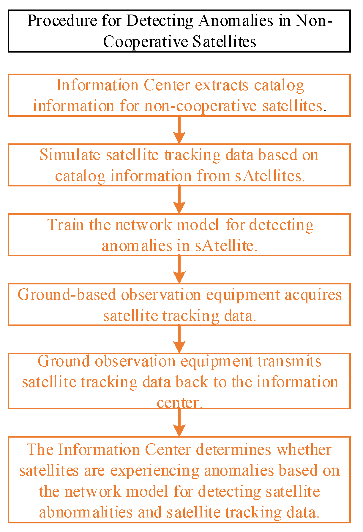
The procedure for detecting anomalies in non-cooperative satellites within this scenario has already been described above. This subsection will detail the process for detecting anomalies in individual cataloged non-cooperative satellites. Before the satellite re-enters an observable region, the information center uses the satellite’s existing catalog information to simulate various tracking observation data, including both normal data and multiple types of anomaly data. Then, we train the pre-built network model for detecting satellite anomalies using simulation data. Once the satellite enters the observable region, it is immediately observed for no more than 20 min using relatively low-performance ground-based observation equipment, and the observation data is transmitted back to the information center. The information center inputs data into the network model to determine whether the satellite is experiencing anomalies. The flowchart for detecting anomalies in non-cooperative satellites is shown in Figure 3.
Even when simultaneously dealing with hundreds of cataloged non-cooperative satellites about to enter the observable region, this process enables rapid detection of satellite anomalies, providing a basis for decision-making regarding the subsequent scheduling and allocation of high-precision ground-based satellite observation equipment.

4. Experiments and Analysis

4.1. Experimental Design

In this section, we validated the model’s effectiveness and its efficiency in detecting anomalies in non-cooperative satellites through numerical experiments conducted on a personal computer. To evaluate the performance of the Attention-based Bi-Directional Minimal GRU model (ABMGRU) in detecting anomalies of cataloged non-cooperative satellites, we designed multiple experimental scenarios, with the primary experimental scenario described in the preceding section. To validate the model’s versatility, after confirming its effectiveness and performance in the primary experimental scenario, we will conduct experiments under different scenario conditions. The primary methods for altering the experimental scenario involve modifying the orbital parameters of non-collaborative satellites or adjusting the magnitude of anomalous forces acting upon them. We compared the Attention-based Bi-Directional Minimal GRU model with several other models and conducted ablation experiments. Performance data for each model in the ablation experiments and other models are presented in the same table, including BPnetwork, LSSVM, LSTM, CNN, GAT, Transformer, GRU, Bi-Directional GRU (BGRU), and Bi-Directional Minimal GRU (BMGRU). The simulation environment is outlined in Table 5.

4.2. Hyperparameter Settings

In the design of Deep Learning (DL), parameters are mainly categorized into model parameters and hyperparameters. Model parameters are the parameters adjusted by the model itself, such as Weight Matrixes and biases in ABMGRU used in this paper. During the model training process, these model parameters are automatically updated internally. Hyperparameters include data-related hyperparameters, model structure hyperparameters, training hyperparameters, regularization hyperparameters, etc. A brief introduction to various hyperparameters is shown in Table 6.
Certain hyperparameters play a crucial and decisive role in the training speed and performance of the entire model. These critical hyperparameters include Learning Rate α , Hidden Layer Size H, Attention Hidden Layer size H a , Batch size B, Number of Epochs e, etc. In this study, we employed a strategy combining dynamic feedback mechanisms with orthogonal experimental designs to adjust and configure these critical hyperparameters. First, we assign each key hyperparameter a relatively broad initial level range based on knowledge and experience to ensure coverage of potential optimal regions. We then select three values within this range for each hyperparameter to conduct orthogonal experiments, yielding the current optimal parameter combination. We then narrow the hyperparameter level range based on this combination and perform orthogonal experiments again. After repeating these steps multiple times, we obtain the relatively optimal combination of key hyperparameters. The specific hyperparameter settings are detailed in Table 7.
To meet the requirements for controlling variables in ablation experiments, the shared hyperparameters of ABMGRU, GRU, BGRU, and BMGRU are identical.

4.3. Model Complexity Analysis

Prior to conducting comparative experiments, all algorithmic models underwent hyperparameter tuning through orthogonal experiments. After determining the key hyperparameters for each model through orthogonal experiments, it is necessary to analyze metrics such as memory consumption, computational complexity, and parameter count for the primary deep learning models. First, BPnetwork and LSSVM models are inherently much simpler than deep learning models, so we will not analyze their complexity-related metrics here. In subsequent result analysis, it can be observed that GAT is not suitable for this scenario, and its computational complexity analysis process is relatively complex. Therefore, we will not conduct its complexity analysis here. CNN has relatively few parameters in each convolutional layer, but each fully connected layer contains a large number of parameters, resulting in a total parameter count of approximately tens of thousands. At the same time, CNN is highly parallelizable in computation, enabling faster model training speeds than LSTM and GRU under comparable parameter counts. The complexity analysis of other major deep learning network models is shown in Table 8.
Table 8 presents the complexity analysis of the five models in the experimental setting of this paper, along with the approximate total number of parameters for their single-layer networks. The total number of parameters for each model includes not only the sum of parameters across its network layers but also the total parameters of the fully connected layer within its classifier and other types of parameters. The total number of parameters for LSTM, GRU, BGRU, BMGRU, and ABMGRU ranges between 0.1 million and 0.5 million, meeting the lightweight criteria for such models. The total number of parameters in the Transformer ranges from 1 million to 5 million, meeting the lightweight criteria for such models. Although the Transformer has significantly more parameters than the other four models, its training process is highly parallelized. Given that the length of the time series data in this scenario does not exceed 100, the Transformer does not suffer from a significant disadvantage in terms of training time. It is undeniable that Transformers consume significant amounts of memory. In the experimental scenario described in this paper, the sequence length of satellite tracking data is relatively short. Therefore, the computational complexity of LSTM, GRU, BGRU, BMGRU, and ABMGRU does not differ significantly. If the shared hyperparameters are identical, the total number of parameters in each BGRU layer equals that in each GRU layer. Meanwhile, the total parameters in each BMGRU layer are reduced by 33% compared to GRU and by 50% compared to LSTM. However, BMGRU requires at least two layers. The parameters in two BMGRU layers exceed those in a single GRU layer by 25%, and their parameter scale is comparable to that of a single LSTM layer. It should be noted that the hyperparameters for LSTM were determined through separate orthogonal experiments, so the hyperparameter H for LSTM in Table 8 differs from the hyperparameter H for various GRU models. Therefore, the actual training time for LSTM may not align with the complexity analysis results for the various models presented here.

4.4. Experimental Results and Analysis

As described in the preceding scenario, the 4400 data samples comprise 11 distinct categories, including one category of non-anomalous data samples and ten categories of anomalous data samples. The normal data samples are assigned label 10, while the 10 types of abnormal samples are assigned labels 0 through 9 in sequence. The anomaly in the data sample manifests as the satellite experiencing a certain abnormal impulse force at a specific moment. The setting time point for the anomaly pulse force is located near the start time point when the satellite enters the observable region, with an interval of 200 s. Assuming the target non-cooperative satellite enters an observable region at time t 0 , and the total duration of satellite tracking data acquired by the ground observation station is T, then the time span of the satellite tracking data ranges from t 0 seconds to t 0 + T seconds. The value of T ranges from 800 to 1200. For Category 9 tracking data, the time point for setting abnormal pulse force is t 0 + 800 ± 10 s. For Category 8, it is t 0 + 600 ± 10 s, and so on down to Category 0, where the time point for setting abnormalities is t 0 1000 ± 10 s. The duration of each abnormal pulse force is 1 s. Category 10 tracking data samples do not set abnormal dynamics. We conduct multiple experiments using different random seeds, including 42 , 102 , 423 , 892 , 1534 , 2409 , 3091 , 3873 , 4682 , 5197 , and select the t-test as the method for significance testing. The performance comparison of different models on the test set is shown in Table 9.
As shown in Table 9, in this experimental scenario, the performance of BPnetwork, LSSVM, and GAT is significantly worse compared to other models. We will no longer consider these three models in subsequent comparative experiments. The statistical significance analysis of performance differences between models is shown in Table 10.
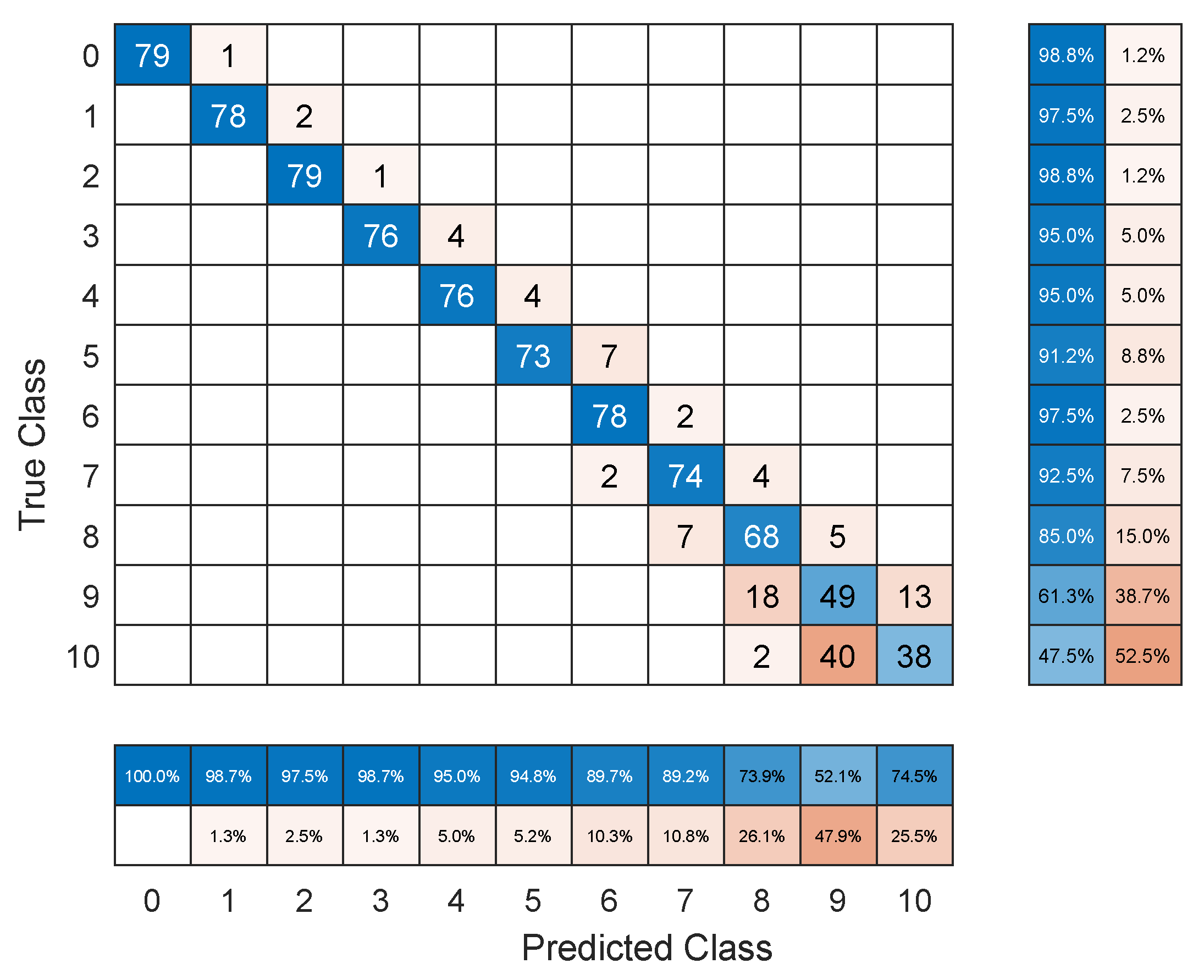
As shown in Table 9 and Table 10, the proposed ABMGRU model achieves an accuracy of 90.3% in this scenario, significantly outperforming all comparison models (p-value < 0.05). Compared to the optimal BMGRU model, ABMGRU demonstrates a 2.9% improvement in accuracy, with this difference being statistically significant (t-statistic = 2.35, p-value < 0.05). Furthermore, the ABMGRU model demonstrated the most outstanding performance across statistical metrics including precision, recall, and F1 score. The training time for the theoretically most complex Transformer model in this experimental scenario was not particularly long. The training time comparison results for the remaining models largely align with the model complexity analysis presented earlier. The additional training time required for ABMGRU is acceptable. The validation set accuracy curves for each model in one independent experiment are shown in Figure 4. The confusion matrix for the ABMGRU in this independent experiment is shown in Figure 5.
As shown in Figure 4, the performance of ABMGRU stabilizes after 10 iterations, allowing for further reduction in model training time by decreasing the number of iterations. Therefore, while ABMGRU outperforms other models in terms of performance, its disadvantage in computational time is further reduced or even negligible. As shown in Figure 5, except for categories 8, 9, and 10, the false alarm rate for satellite tracking data in other categories is extremely low. Analysis of the data structure for each category reveals that this experimental outcome stems from the data simulation method rather than inherent flaws in the model itself. In this experimental scenario, the actual time span of the raw data ranges from t 0 to t 0 + T seconds, where T is between 800 and 1200 s. Each data sample, after preprocessing, contains 100 time steps spanning from t 0 to t 0 + 1000 s. According to the satellite’s anomaly force configuration rules in this scenario, the anomaly pulse force configuration node for the 9th category data sample is set at t 0 + 800 ± 10 s. Therefore, the characteristics of the 9th category data sample prior to 800 s are nearly identical to those data samples without abnormalities. Meanwhile, the data for some samples after t 0 + 800 s was obtained through preprocessing using Kalman filtering. In summary, the differences between the data samples in category 9 and the normal data samples (i.e., category 10) are significantly smaller, making the task of distinguishing between them considerably more challenging, which can be directly observed from the Confusion Matrix of ABMGRU. Such issues arise from the methods of data simulation and preprocessing employed in simulation experiments, rather than from inherent flaws in the model itself, and thus have minimal impact in practical applications.

4.5. Verification of the General Applicability of ABMGRU and Analysis

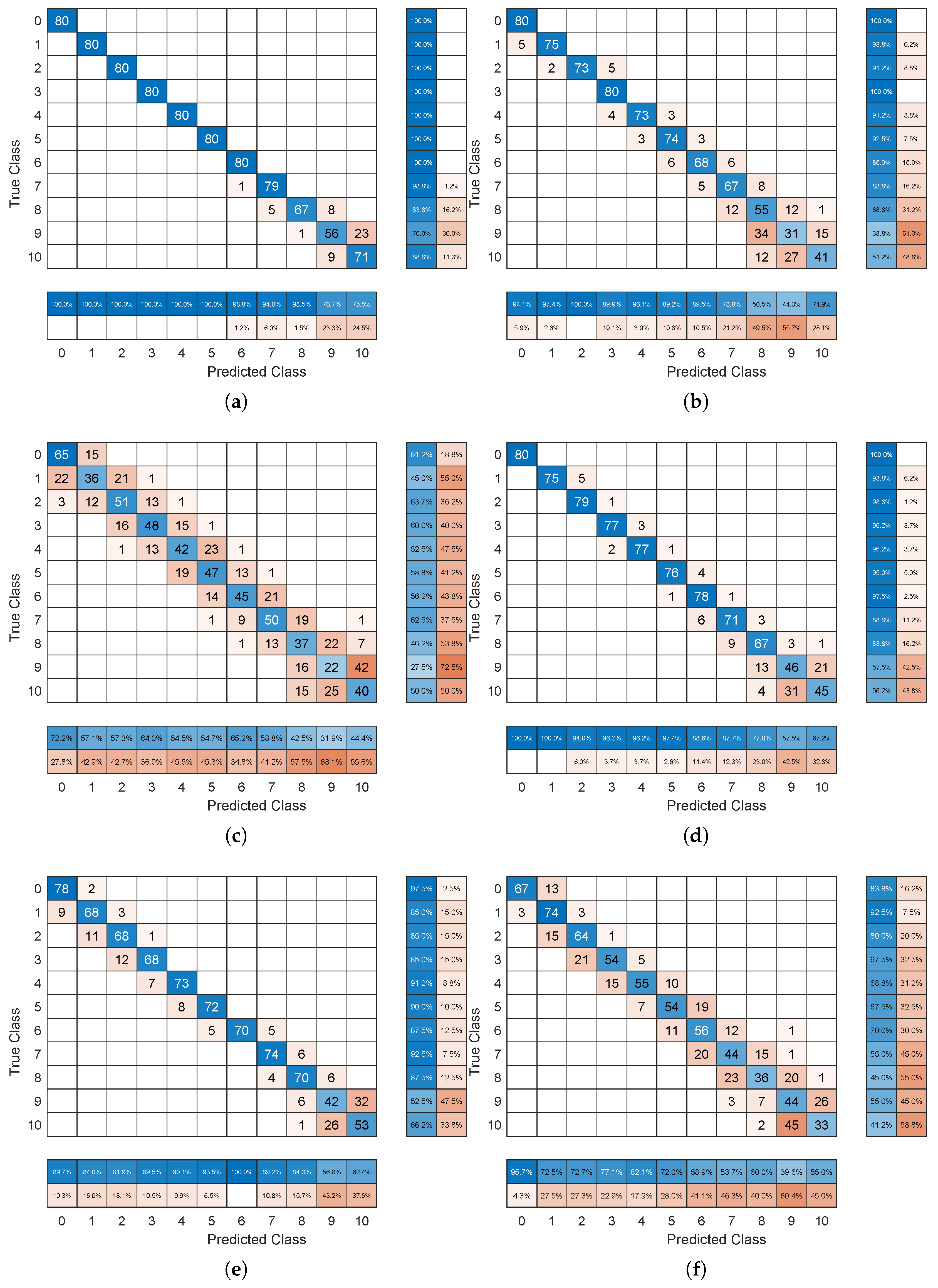
In this section, we will validate the general applicability of the ABMGRU model under other experimental conditions. To modify the experimental scenario conditions in this paper, adjustments can be made in three areas: first, altering the orbital parameters of the satellite; second, modifying the location parameters of the ground observation stations; and third, changing the values of the anomalous forces acting on the satellite. The first two methods directly affect the entire satellite tracking observation data, altering the satellite’s flight path throughout the observable region. The third method directly impacts the model’s ability to detect anomalies in non-cooperative satellites. The type of impact on satellite tracking observation data caused by altering any parameter value of the satellite’s orbital six-element set or changing any position parameter value of a ground observation station is similar. Therefore, in verifying the universal applicability of the model in this subsection, we selected either modifying the semi-major axis of the satellite’s orbital parameters or altering the magnitude of the anomalous forces acting on the satellite to change the experimental scenario. We have currently designed six new experimental scenarios to validate the model’s universality. The first three experimental scenarios maintain the satellite’s semi-major axis constant while modifying the magnitude of the anomalous impulse force applied to the satellite to 2.5 N, 1.5 N, and 1 N, respectively. The latter three scenarios keep the magnitude of the anomalous impulse force constant while modifying the satellite’s semi-major axis to 6,928,137 m, 6,978,137 m, and 7,078,137 m. After multiple independent experiments, the validation set accuracy curves for each model across various experimental scenarios are shown in Figure 6. The confusion matrices for ABMGRU across different experimental scenarios are presented in Figure 7.
Based on the performance of ABMGRU across multiple experimental scenarios, the difficulty of detecting anomalies in cataloged non-cooperative satellites increases as the magnitude of the anomalous forces acting upon them decreases, and also as the semi-major axis of the non-cooperative satellite grows. We kept the total observation duration unchanged when altering the experimental scenario. In reality, the observable time window for the satellite increases with the growth of its semi-major axis. This occurs because a longer semi-major axis results in reduced linear and angular velocities, while simultaneously extending the satellite’s flight path. Therefore, the longer the semi-major axis of a non-cooperative satellite, the longer the time span of its tracking observation data sample should be; otherwise, the model’s ability to detect anomalies will be compromised. These experimental results align with real-world conditions, demonstrating not only the effectiveness of ABMGRU in diverse experimental settings but also its superiority over other lightweight models.

5. Conclusions

This paper proposes an Attention-based Bi-Directional Minimal GRU network model for detecting anomalies in cataloged non-cooperative satellites. This model can quickly determine whether a cataloged non-cooperative satellite is anomalous once it enters an observable region, and roughly identify the type of anomaly. This provides decision-making support for determining whether to allocate high-precision observation equipment to track and monitor the satellite. A dedicated model is trained for each satellite, with the model pre-built and pre-trained. The dataset used for model training was simulated based on STK software and existing catalog information for non-cooperative satellites. Since hundreds of models need to be stored, trained, and utilized simultaneously in practical applications, this scenario also imposes certain requirements for model lightweighting. This paper’s Attention-based Bi-Directional Minimal GRU significantly reduces model complexity by simplifying the GRU architecture without sacrificing much expressiveness. It then designs a bidirectional GRU network structure to learn more complete feature information from time series data. Finally, it incorporates an attention mechanism to identify key features in satellite tracking data. Despite its relatively lightweight structure, this model demonstrates strong capability in detecting anomalies in cataloged non-cooperative satellites. Extensive experiments demonstrate that the Attention-based Bi-Directional Minimal GRU outperforms other lightweight algorithms. It exhibits a certain level of detection capability for relatively minor satellite anomalies, but requires designing the time span for tracking and observing satellites tailored to specific scenarios.
Our work primarily addresses two critical practical challenges. First, under the current conditions of explosive growth in non-cooperative satellites in space, how to most effectively utilize existing satellite observation resources. Second, under limited computational resources, how to maximize the performance of models for detecting satellite anomalies.
This study also has certain limitations. First, since the actual cataloging information of satellites cannot be disclosed externally, the research was primarily conducted using simulation data, lacking experimental verification based on real satellite cataloging information. Second, the number of categories of satellite anomaly propulsion far exceeds ten. The types of minor anomalous propulsion forces considered in this study are not sufficiently comprehensive. Beyond different types of minor anomalous impulse forces, satellites may also experience numerous other types of anomalous propulsion, such as continuous minor thrust generated by electric propulsion or cold gas thrusters. Finally, although we progressively increased the satellite’s semi-major axis in experimental verification, the experiments remain confined to low-Earth orbit conditions. Although anomaly detection for high-orbit satellites is similar to that for low-orbit satellites, their slow movement across ground station star charts necessitates satellite tracking data spanning significantly longer time periods for detecting high-orbit satellite anomaly dynamics. This leads to noticeable changes in computational complexity, parameter counts, and training times across different models.
This paper can be extended in several directions. First, the sheer variety of non-cooperative satellite anomalies is vast, and this paper simulated only a limited number of satellite anomaly scenarios. Future research could simulate data from more typical satellite anomalies to train the model, thereby enhancing its ability to detect satellite anomalies. Second, when designing the Attention-based Bi-Directional Minimal GRU network model, we constructed only two layers of GRU to reduce model complexity. However, even adding several more GRU layers would not significantly increase the overall model complexity. Future research could improve the network architecture of the Attention-based Bi-Directional Minimal GRU or explore more effective network models. Finally, this research can be gradually extended from low-orbit satellites to high-orbit satellites.

Author Contributions

Writing—original draft, P.L.; supervision and resources, Y.J.; project administration, X.W.; data curation, B.S.; validation, X.P. All authors have read and agreed to the published version of the manuscript.

Funding

This work was supported by the National Natural Science Foundation of China [Grant Number 62503487], National University of Defense Technology Scientific Research Fund for Young Scholars’ Independent Innovation [Grant Number ZK25-60], the National University of Defense Technology Independent Innovation Research Fund [Grant Number 24-ZZCX-GZZ-01-01], the National Key Laboratory of Space Intelligent Control [Grant Number 2024-CXPT-GF-JJ-012-16], and National Key Laboratory of Spacecraft Thermal Control Open Fund [Grant Number NKLST-JJ-005].

Data Availability Statement

The datasets presented in this article are not readily available because satellites and ground observation stations are both high-value assets, and authentic satellite tracking and observation data are extremely valuable and confidential. Requests to access the datasets should be directed to panxiaogang_nudt@163.com.

Conflicts of Interest

The authors declare no conflicts of interest.

Abbreviations

The following abbreviations are used in this manuscript:
ARAutoregression
MAMoving Average
ARMAAuto-Regression and Moving Average
ARIMAAutoregressive Integrated Moving Average
VARVector Autoregression
VARMAVector Autoregressive Moving Average
VARIMAVector Autoregressive Integrated Moving Average
BPnetworkBack Propagation Neural Networks
LSSVMLeast Squares Support Vector Machines
RNNRecurrent Neural Networks
LSTMLong Short-Term Memory
GRUGated Recurrent Unit
GCNGraph Convolutional Networks
GATGraph Attention Networks
BGRUBi-Directional Gated Recurrent Unit
BMGRUBi-Directional Minimal Gated Recurrent Unit
ABMGRUAttention-based Bi-Directional Minimal Gated Recurrent Unit
STKSatellite Tool Kit
Mmillion
NaNNot a Number

References

  1. Xiao, J.; Fu, X. Space Security:A Shared Responsibility. Beijing Rev. 2025, 17, 28–29. [Google Scholar]
  2. Jia, Q.; Xiao, J.; Bai, L.; Zhang, Y.; Zhang, R.; Feroskhan, M. Space situational awareness systems: Bridging traditional methods and artificial intelligence. Acta Astronaut. 2025, 228, 321–330. [Google Scholar] [CrossRef]
  3. Kazemi, S.; Azad, N.; Scott, K.; Oqab, H.; Dietrich, G. Orbit determination for space situational awareness: A survey. Acta Astronaut. 2024, 222, 272–295. [Google Scholar] [CrossRef]
  4. Hu, Y.; Li, K.; Liang, Y.; Chen, L. Review on strategies of space-based optical space situational awareness. J. Syst. Eng. Electron. 2021, 32, 1152–1166. [Google Scholar] [CrossRef]
  5. Zhong, J. Space Strategic Competition and Rivalry are Intensifying. Renming Luntan·Xueshu Qianyan 2020, 16, 22–28. [Google Scholar]
  6. Albrecht, M.; Graziani, P. Congested Space. Space News Int. 2016, 27, 22–23. [Google Scholar]
  7. Marcussen, E. Congested and Contested Spaces. Acts Aid 2023, 1, 248–301. [Google Scholar]
  8. Laura, S. Is the Security Space too Congested. Secur. Distrib. Mark. 2016, 46, 58–66. [Google Scholar]
  9. Han, H.; Dang, Z. Threat assessment of non-cooperative satellites in interception scenarios: A transfer window perspective. Defence Technol. 2025. [Google Scholar] [CrossRef]
  10. Yuan, W.; Xia, Q.; Qian, H.; Qiao, B.; Xu, J.; Xiao, B. An intelligent hierarchical recognition method for long-term orbital maneuvering intention of non-cooperative satellites. Adv. Space Res. 2025, 75, 5037–5050. [Google Scholar] [CrossRef]
  11. Wu, G.; Wang, H.; Pedrycz, W.; Li, H.; Wang, L. Satellite observation scheduling with a novel adaptive simulated annealing algorithm and a dynamic task clustering strategy. Comput. Ind. Eng. 2017, 113, 576–588. [Google Scholar] [CrossRef]
  12. Chahal, A.; Addula, S.; Jain, A.; Gulia, P.; Gill, N.; Bala, V. Systematic Analysis based on Conflux of Machine Learning and Internet of Things using Bibliometric analysis. J. Intell. Syst. Internet Things 2024, 13, 196–224. [Google Scholar]
  13. Shawn, M.; Marco, C.; Marcello, R. Simulations of Multiple Spacecraft Maneuvering with MATLAB/Simulink and Satellite Tool Kit. J. Aerosp. Inf. Syst. 2013, 10, 348–358. [Google Scholar] [CrossRef]
  14. Zhao, Y.; Song, Y.; Wu, L.; Liu, P.; Lv, R.; Ullah, H. Lightweight micro-motion gesture recognition based on MIMO millimeter wave radar using Bidirectional-GRU network. Neural Comput. Appl. 2023, 35, 23537–23550. [Google Scholar] [CrossRef]
  15. Guo, H.; Liu, J.; Li, A.; Zhang, J. Earth observation satellite data receiving, processing system and data sharing. Int. J. Digit. Earth 2012, 3, 241–250. [Google Scholar] [CrossRef]
  16. Schefels, C.; Schlag, L.; Helmsauer, K. Synthetic satellite telemetry data for machine learning. CEAS Space J. 2025, 17, 863–875. [Google Scholar] [CrossRef]
  17. Li, X.; Li, Y.; Zhang, K.; Fu, Y.; Zhang, W. Precise orbit determination for LEO constellation based on onboard GNSS observations, inter-satellite links and ground tracking data. GPS Solut. 2025, 29, 107. [Google Scholar] [CrossRef]
  18. Kaseris, M.; Kostavelis, I.; Malassiotis, S. A Comprehensive Survey on Deep Learning Methods in Human Activity Recognition. Mach. Learn. Knowl. Extr. 2024, 6, 842–876. [Google Scholar] [CrossRef]
  19. Barandas, M.; Folgado, D.; Fernandes, L. TSFEL: Time series feature extraction library. SoftwareX 2020, 11, 100456. [Google Scholar] [CrossRef]
  20. Kini, B.; Sekhar, C. Large margin mixture of AR models for time series classification. Appl. Soft Comput. 2013, 13, 361–371. [Google Scholar] [CrossRef]
  21. Zhuang, Y.; Li, D.; Yu, P.; Li, W. On buffered moving average models. J. Time Ser. Anal. 2025, 46, 599–622. [Google Scholar] [CrossRef]
  22. Raza, S.; Majid, A. Maximum likelihood estimation of the change point in stationary state of auto regressive moving average (ARMA) models, using SVD-based smoothing. Commun. Stat.-Theory Methods 2022, 51, 7801–7818. [Google Scholar]
  23. Sayed Rahmi, K.; Athar Ali, K. A Bayesian Prediction for the Total Fertility Rate of Afghanistan Using the Auto-regressive Integrated Moving Average (ARIMA) Model. Reliab. Theory Appl. 2023, 18, 980–997. [Google Scholar]
  24. Yang, H.; Pan, Z.; Tao, Q. Online learning for vector auto-regressive moving-average time series prediction. Neurocomputing 2018, 315, 9–17. [Google Scholar] [CrossRef]
  25. Gong, X.; Liu, X.; Xiong, X. Non-Gaussian VARMA model with stochastic volatility and applications in stock market bubbles. Chaos Solitons Fractals 2019, 121, 129–136. [Google Scholar] [CrossRef]
  26. Zhang, Y.; Cheng, C.; Cao, R. Multivariate probabilistic forecasting and its performance’s impacts on long-term dispatch of hydro-wind hybrid systems. Appl. Energy 2021, 283, 116243. [Google Scholar] [CrossRef]
  27. Davesh, M.; Shen, J.; Yin, Q. Perverse filtrations and Fourier transforms. Acta Math. 2025, 234, 1–69. [Google Scholar] [CrossRef]
  28. Liu, Y.; Zhang, H.; Wei, X.; Li, M. Back Propagation Neural Network-Enhanced Generative Model for Drying Process Control. Informatica 2025, 49, 63–76. [Google Scholar] [CrossRef]
  29. Wang, M.; Zhong, C.; Yue, K.; Zheng, Y.; Jiang, W.; Wang, J. Modified MF-DFA Model Based on LSSVM Fitting. Fractal Fract. 2024, 8, 320. [Google Scholar] [CrossRef]
  30. Gupta, M.; Chandra, P. A comprehensive survey of data mining. Int. J. Inf. Technol. 2020, 12, 1243–1257. [Google Scholar] [CrossRef]
  31. Xiao, H.; Xu, M.; Zhang, Y.; Weng, S. Stability of Stochastic Delayed Recurrent Neural Networks. Mathematics 2025, 13, 2310. [Google Scholar] [CrossRef]
  32. Hochreiter, S.; Schmidhuber, J. Long short-term memory. Neural Comput. 1997, 9, 1735–1780. [Google Scholar] [CrossRef]
  33. Tjandra, A.; Sakti, S.; Manurung, R.; Adriani, M.; Nakamura, S. Gated Recurrent Neural Tensor Network. In Proceedings of the 2016 International Joint Conference on Neural Networks (IJCNN), Vancouver, BC, Canada, 24–29 July 2016. [Google Scholar]
  34. LeCun, Y.; Bottou, L.; Bengio, Y. Gradient-based learning applied to document recognition. Proc. IEEE 1998, 86, 2278–2324. [Google Scholar] [CrossRef]
  35. Vaswani, A.; Shazeer, N.; Parmar, N. Attention is all you need. Adv. Neural Inf. Process. Syst. 2017, 30, 5998–6008. [Google Scholar]
  36. Wu, Z.; Pan, S.; Chen, F. A comprehensive survey on graph neural networks. lEEE Trans. Neural Netw. Learn. Syst. 2020, 32, 4–24. [Google Scholar] [CrossRef]
  37. Latif-Martínez, H.; Suárez-Varela, J.; Cabellos-Aparicio, A.; Barlet-Ros, P. GAT-AD: Graph Attention Networks for contextual anomaly detection in network monitoring. Comput. Ind. Eng. 2025, 200, 110830. [Google Scholar] [CrossRef]
  38. Håkon, G.; Håkon, T. Ensemble Kalman filter with precision localization. Comput. Stat. 2025, 40, 2781–2805. [Google Scholar]
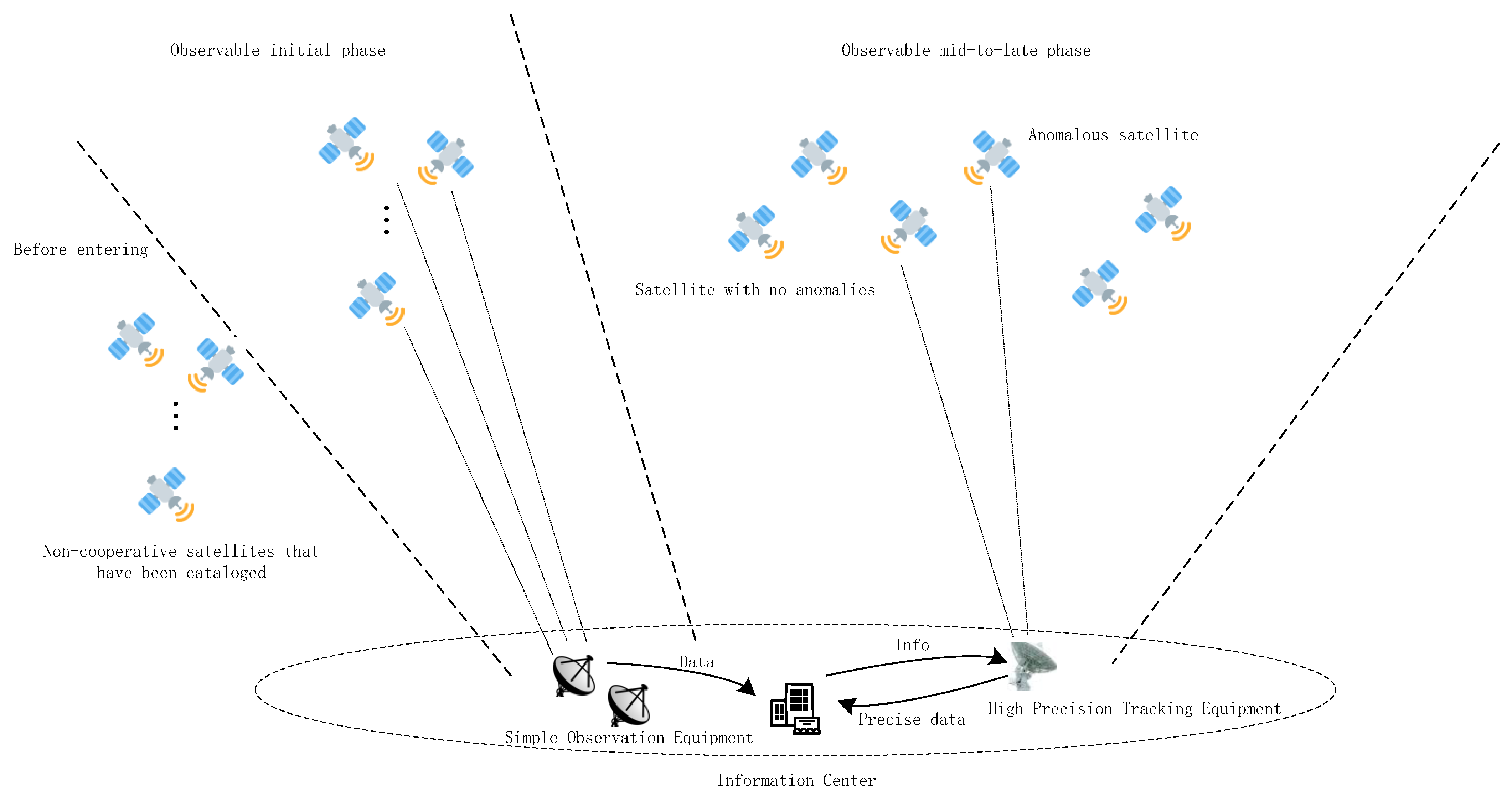
Figure 1. Schematic diagram of the experimental scenario.
Asi 08 00163 g001
Figure 2. The network architecture diagram of the Attention-based Bi-Directional Minimal GRU model.
Asi 08 00163 g002
Figure 3. Procedure for detecting anomalies in non-cooperative satellites.
Asi 08 00163 g003
Figure 4. Validation set accuracy curves for each model.
Asi 08 00163 g004
Figure 5. Confusion Matrix of ABMGRU. The blue diagonal cells represent correct classifications, and the red off-diagonal cells represent misclassifications. The intensity of the color corresponds to the number of instances in each cell.
Asi 08 00163 g005
Figure 6. Validation set accuracy curves for each model under different experimental conditions. (a) The magnitude of the pulse force is 2.5 N. The semi-major axis of the orbit is 6,878,137 m. (b) The magnitude of the pulse force is 1.5 N. The semi-major axis of the orbit is 6,878,137 m. (c) The magnitude of the pulse force is 1 N. The semi-major axis of the orbit is 6,878,137 m. (d) The magnitude of the pulse force is 2 N. The semi-major axis of the orbit is 6,928,137 m. (e) The magnitude of the pulse force is 2 N. The semi-major axis of the orbit is 6,978,137 m. (f) The magnitude of the pulse force is 2 N. The semi-major axis of the orbit is 7,078,137 m.
Asi 08 00163 g006
Figure 7. Confusion matrix of ABMGRU under different experimental conditions, using the same color mapping as in Figure 5. (a) The magnitude of the pulse force is 2.5 N. The semi-major axis of the orbit is 6,878,137 m. (b) The magnitude of the pulse force is 1.5 N. The semi-major axis of the orbit is 6,878,137 m. (c) The magnitude of the pulse force is 1 N. The semi-major axis of the orbit is 6,878,137 m. (d) The magnitude of the pulse force is 2 N. The semi-major axis of the orbit is 6,928,137 m. (e) The magnitude of the pulse force is 2 N. The semi-major axis of the orbit is 6,978,137 m. (f) The magnitude of the pulse force is 2 N. The semi-major axis of the orbit is 7,078,137 m.
Asi 08 00163 g007
Table 1. Core structural elements of satellite observation data and their definitions.
Core ElementsDefinition
TimestampPrecisely record the moment data is captured.
Satellite IdentifierClearly indicate which satellite the data originates from.
Ground Station IdentifierRecord which ground station received this data.
Telemetry data [16]A “health check report” reflecting the satellite platform and payload’s operational status and performance parameters.
Tracking Data [17]Core raw measurement data used for precisely determining satellite position and velocity.
Table 2. Definitions of Key Characteristics of Multivariate Time Series.
Key CharacteristicsDefinition
Time dependenceAlso known as autocorrelation or temporal dependence, it refers to a statistically significant correlation between the current observation in a time series and its past observation (s) at one or more preceding time points. In a multivariate context, this dependency exists both within individual variables (univariate autocorrelation) and between different variables (cross-correlation).
Spatial dependenceSpatial dependence specifically refers to the interdependent relationship between observations of different variables (dimensions) at the same or different time points within a multivariate time series. It describes the “lateral” interactions or influences between variables.
Spectral characteristicsSpectral characteristics describe the properties of a time series in the frequency domain. They decompose the time series into sinusoidal and cosine wave components of different frequencies and analyze the intensity of these frequency components.
Noise characteristicsNoise characteristics refer to the unpredictable, randomly fluctuating components within a time series. They represent the portion of the data that cannot be explained by the model and are typically regarded as “error” or “disturbance”.
Shape characteristicsShape characteristics focus on the morphology, contours, and structure of local segments within a time series. They provide an intuitive description of sub-sequences, such as ascending, descending, peaks, troughs, plateaus, and so forth.
Similarity featuresSimilarity features are used to quantify the degree of similarity in overall or local patterns between two time series (or two subsequences).
Table 3. A review of deep learning models for multivariate time series data mining.
ModelBrief PrincipleAdvantageDefect
BPnetworkFlatten the input multivariate time series into a one-dimensional vector. Subsequent operations follow the same procedure as classic BPnetwork.Strong nonlinear fitting capability. High flexibility.Flattening operations disrupt the temporal relationships within the data. Input length must be fixed.
LSSVMFlatten the input data. Manually extract features to form feature vectors.High computational efficiency. Few parameters.Sensitive to outliers. Overly reliant on feature engineering, making it difficult to extract features directly from raw time series data.
RNNProcess time step data sequentially. Errors propagate backward through time.Natural sequence modeling capability. Does not require fixed input data length.It is prone to issues such as vanishing gradients or exploding gradients. The theoretical advantages of RNN are almost entirely realized through its variant algorithms.
LSTMVariant algorithms of RNNs. Utilizing unique mechanisms to selectively remember or forget information.Exceptional long-term modeling capabilities. Mitigates the issues of vanishing gradients or exploding gradients in RNN.Computational costs are high. Model training is time-consuming.
GRUA variant of LSTM with a simpler structure.Faster training and inference speeds.May not perform as well as LSTM when handling complex tasks.
CNNTreating multivariate time series as pseudo-images for processing.Strong local pattern extraction capability. Flexible and efficient architecture.Long-term dependency extraction capability is weak.
TransformerModeling global dependencies through self-attention mechanisms.Powerful global modeling capabilities. Fully parallelized computation significantly accelerates training speed.Extremely high computational complexity. High memory requirements.
GCNModel multi-dimensional time series as graphs. Graph convolution operations aggregate neighboring information.A fresh perspective. Applicable to non-Euclidean data. Explicitly model relationships between variables.Performance is highly dependent on the quality of adjacency matrix. Graph structure in standard GCN is static.
GATDynamically learn the strength of relationships between variables through the Graph Attention Mechanism.GAT represents a revolutionary evolution of GCN, freeing it from dependence on a predefined adjacency matrix. Attention coefficient calculations can be parallelized, resulting in significantly faster training speeds.Similar to GCN, it requires relatively complex interrelationships among variables in multivariable time series; otherwise, its performance may be inferior to traditional models.
Table 4. Abbreviation of symbols.
SymbolDescription
tTime step t, t N .
DThe size D of the input dimension for each time step, D N + .
z t Update Gate Vector at time step t, z t R H .
r t Reset Gate Vector at time step t, r t R H .
h t Hidden State Vector at time step t, h t R H , (In Bi-Directional Minimal GRU, h t R 2 H ).
h t Hidden State Vector of the forward GRU at time step t, h t R H .
h t Hidden State Vector of the backward GRU at time step t, h t R H .
hh is the hidden state sequence containing all time step information. h = h 1 , h 2 , , h T , h R H × T .
HThe dimension size of the hidden layer h t .
H a H a is the dimension of the attention network and is a hyperparameter.
h ˜ t Candidate Hidden State Vector at time step t, h ˜ t R H .
σ σ represents the sigmoid function.
XX is the input sequence, X = x 1 , x 2 , , x T , X R D × T .
x t Raw data vector at time step t, x t R D .
W z Weight Matrix of Update Gate, W z R H × H + D .
W r Weight Matrix of Reset Gate, W r R H × H + D .
W h ˜ Weight Matrix of Candidate Hidden State, W h ˜ R H × H + D .
W a Weight Matrix of Attention Mechanism, W a R H a × 2 H .
W c Weight Matrix of Classifier, W c R C × 2 H .
b z Bias of Update Gate, b z R H .
b r Bias of Reset Gate, b r R H .
b h ˜ Bias of Candidate Hidden State, b h ˜ R H .
b a Bias of Attention Mechanism, b a R H a .
b c Bias of Classifier, b c R C .
e t e t converted from h t . It can be regarded as “energy” at time step t, e t R H a .
u a The context vector u a can be regarded as a “query” vector used to identify significant hidden states, u a R H a .
α t α t is the attention weight at time step t, α t 0 , 1 , α t = 1 .
cA fixed-size Context Vector focused on key information, c R 2 H .
CTotal number of categories for satellite tracking observation data.
y ^ The final probability distribution obtained through the model. y ^ R C .
LInput Sequence Length.
d m o d e l Hidden Feature Dimensions of Transformer.
Table 5. Details the simulation environment configuration.
ItemDescription
Processor *11th Gen Intel(R) Core(TM) i5-11400H @ 2.70 GHz (2.69 GHz)
RAM *16.0 GB
OS *Windows11 (64-bit)
Python versionPython 3.9
* ASUS, Taipei, Taiwan, China.
Table 6. Brief introduction to various hyperparameters.
ClassificationKey Members
Data-related hyperparametersThe Length of the Sequence, Number of Features, Number of Classes
Model structure hyperparametersHidden Layer Size, Number of Layers, Attention Hidden Layer Size
Training hyperparametersBatch size, Learning rate, Number of Epochs
Regularization hyperparametersDropout Rate, Weight Decay
Table 7. Hyperparameter settings.
ParameterValueDescription
Learning Rate0.001Learning rate for the Adam optimizer
Number of Epochs25Total number of iterations in model training
OptimizerAdamThe type of optimizer used by the model
Loss FunctionCategorical crossentropythe type of loss function used in the model
Batch Size128The total number of samples drawn during each iteration of model training
Dropout Rate0.3The ratio of parameters discarded during output at each network layer
Weight Decay0.0001L2 regularization coefficient
Number of Layers2Total number of layers in the GRU network
Hidden Layer Size64Dimension of the GRU Hidden Layer
Attention Hidden Layer size32Dimension of the hidden layer in the attention mechanism
Table 8. Complexity analysis of each layer in each model.
ModelComputational ComplexityNumber of Network ParametersTotal per Layer (Approx.)
Transformer O L 2 × d m o d e l + L × d m o d e l 2 12 d m o d e l 2 + 13 d m o d e l 1 M
LSTM O L × H × H + D 4 H H + D + 1 0.066 M
GRU O L × H × H + D 3 H H + D + 1 0.05 M
BGRU O L × H × H + D 3 H H + D + 1 0.05 M
BMGRU O L × H × H + D 2 H H + D + 1 0.033 M
ABMGRU O L × H × H + D + L 2 × H a × H 2 H H + D + 1 + 0.5 H a 3 H + 1 0.043 M
Table 9. The performance comparison of different models on the test set.
ModelAccuracyPrecisionRecallF1Time (s)
BPnetwork0.668  ±  0.0130.669 ± 0.0140.668 ± 0.0130.665 ± 0.0153.355 ± 0.694
LSSVM0.16 ± 0.0120.151 ± 0.0140.16  ± 0.0110.15 ± 0.0101.066 ± 0.127
GAT0.599 ± 0.0190.568 ± 0.0530.599 ± 0.0200.569 ± 0.01427.745 ± 2.834
Transformer0.829 ± 0.0180.831 ± 0.0150.829 ± 0.0190.82 ± 0.013101.689 ± 6.142
LSTM0.847 ± 0.0090.851 ± 0.0140.847 ± 0.0110.844 ± 0.011148.12 ± 6.137
CNN0.784 ± 0.0150.783 ± 0.0150.784 ± 0.0160.781 ± 0.01219.026 ± 0.283
GRU0.837 ± 0.0330.848 ± 0.0210.837 ± 0.0320.839 ± 0.02623.538 ± 2.363
BGRU0.866 ± 0.0270.878 ± 0.0230.877 ± 0.0250.874 ± 0.01791.776 ± 6.756
BMGRU0.874 ± 0.0230.884 ± 0.0170.874 ± 0.0220.878 ± 0.01545.016 ± 2.353
ABMGRU0.903 ± 0.0190.904 ± 0.0180.903 ± 0.0220.902 ± 0.01786.083 ± 4.874
Results are reported as “mean ± 95% confidence interval radius” based on 10 replicate experiments.
Table 10. Statistical significance of performance differences between models.
ModelDifference in Meanst-Statisticp-ValueSignificance
ABMGRU vs. Transformer7.4%6.98 p < 0.05 significant
ABMGRU vs. LSTM5.6%6.24 p < 0.05 significant
ABMGRU vs. CNN11.9%11.97 p < 0.05 significant
ABMGRU vs. GRU6.6%4.37 p < 0.05 significant
ABMGRU vs. BGRU3.7%2.88 p < 0.05 significant
ABMGRU vs. BMGRU2.9%2.35 p < 0.05 significant
Based on 10 independent experiments, when t-statistic > 1.833 (one-tailed test), it indicates that the performance difference between models is statistically significant (p-value < 0.05).
Disclaimer/Publisher’s Note: The statements, opinions and data contained in all publications are solely those of the individual author(s) and contributor(s) and not of MDPI and/or the editor(s). MDPI and/or the editor(s) disclaim responsibility for any injury to people or property resulting from any ideas, methods, instructions or products referred to in the content.