Article

LCxNet: An Explainable CNN Framework for Lung Cancer Detection in CT Images Using Multi-Optimizer and Visual Interpretability

Department of Computer Engineering, College of Engineering, University of Basrah, Basrah 61004, Iraq
*
Author to whom correspondence should be addressed.
Appl. Syst. Innov. 2025, 8(5), 153; https://doi.org/10.3390/asi8050153
Submission received: 1 June 2025 / Revised: 29 July 2025 / Accepted: 7 October 2025 / Published: 15 October 2025
(This article belongs to the Special Issue Advancements in Deep Learning and Its Applications)

Abstract

Lung cancer, the leading cause of cancer-related mortality worldwide, necessitates better methods for earlier and more accurate detection. To this end, this study introduces LCxNet, a novel, custom-designed convolutional neural network (CNN) framework for computer-aided diagnosis (CAD) of lung cancer. The IQ-OTH/NCCD lung CT dataset, which includes three different classes—benign, malignant, and normal—is used to train and assess the model. The framework is implemented using five optimizers, SGD, RMSProp, Adam, AdamW, and NAdam, to compare the learning behavior and performance stability. To bridge the gap between model complexity and clinical utility, we integrated Explainable AI (XAI) methods, specifically Grad-CAM for decision visualization and t-SNE for feature space analysis. With accuracy, specificity, and AUC values of 99.39%, 99.45%, and 100%, respectively, the results demonstrate that the LCxNet model outperformed the state-of-the-art models in terms of diagnostic performance. In conclusion, this study emphasizes how crucial XAI is to creating trustworthy and efficient clinical tools for the early detection of lung cancer.

1. Introduction

Lung cancer ranks among the most prevalent and lethal forms of cancer globally, according to the World Health Organization (WHO) [1]. Low-dose CT (LDCT) is the cornerstone of early lung cancer detection, but its use has escalated radiologists’ diagnostic workload [2].
Noteworthy, since small pulmonary nodules and early-stage malignancies are frequently overlooked by ordinary chest X-rays (CXR); CT scans are beneficial in detecting these conditions. Besides this, CT imaging provides physicians with comprehensive anatomical data that is capable of differentiating between benign and malignant lesions based on features such as size, shape, edges, and growth rate. This would certainly assist clinicians making more informed decisions regarding additional research or therapy [3].
The two main categories of lung cancer are small cell lung cancer (SCLC) and non-small cell lung cancer (NSCLC), each with distinct biological behaviors and treatment approaches [4]. The vast majority (over 80%) of lung cancer deaths are driven by tobacco smoking. In contrast, lung cancer in nonsmokers typically results from exposure to passive smoke, radon, or environmental pollution [5].
In clinical practice, CAD systems are pivotal in supporting radiologists. They automate image analysis to enhance early detection of malignant lesions, improve diagnostic consistency, accelerate workflow, and extract quantitative imaging biomarkers imperceptible to the human eye [6].
Nevertheless, the immense data volumes from essential diagnostic tools like CT and PET-CT complicate interpretation, highlighting the need for sophisticated analytical solutions [7]. This is where artificial intelligence (AI), particularly deep learning (DL), becomes pivotal. By leveraging multilayered neural networks to learn from vast datasets, AI is revolutionizing medical image analysis and continuously improving diagnostic performance [8].
In contrast, Machine Learning (ML), a broad field that includes deep learning, is based on algorithms. According to patterns found in the data, machine learning algorithms examine the data, derive insights, and make decisions. Feature engineering, in which features are manually created from raw data using domain expertise, is frequently used in traditional machine learning techniques. In fields like healthcare, where automated feature learning may not always be practical or dependable, this manual method is beneficial [9].
In medical imaging, convolutional neural networks (CNNs) excel at precise image segmentation and feature extraction [10]. These superior outputs enhance the performance of traditional classifiers such as Support Vector Machines (SVMs) and Artificial Neural Networks (ANNs). This synergistic combination facilitates earlier and more accurate detection of cancerous nodules, accelerating diagnosis and improving patient outcomes [11].
For example, CovLscan is a multi-modal ensemble architecture that utilizes DL and Transfer Learning (TL) to address epistemic uncertainty in the identification of lung disease from CT scans and CXR [12]. A CNN model was developed using the IQ-OTH/NCCD dataset to automatically classify chest CT scans into benign, malignant, and normal categories, thereby enhancing early detection and improving patient outcomes, representing a significant advancement in computer-aided lung cancer diagnosis [13].
For tumor localization tasks in CT and PET-CT scans, the YOLOv8 model (You Only Look Once) acts as a single-shot detection model. It identifies suspicious regions with bounding boxes and passes them to a CNN for fine-grained classification. The workflow includes preprocessing, detection, classification, and post-processing. Advantages include real-time performance, modular design, and multi-modal compatibility, making it ideal for clinical triage [14]. Researchers also presented a hybrid DL model, which combines CNNs and Vision Transformers (ViTs) to detect lung cancer using CT scans. The remarkable accuracy of this innovative approach demonstrates its potential to improve diagnostic methods [15].
To assess model trustworthiness and interpretation, a study evaluated several pre-trained CNN architectures on CT scan datasets, focusing on their ability to generalize across different patient cohorts and imaging conditions. They applied Local Interpretable Model-Agnostic Explanations (LIME) to generate localized surrogate models. These models highlight image areas or features influencing predictions, which is crucial for distinguishing benign from malignant nodules and is vital for clinical trust and acceptance [16].
This study introduces a novel explainable CNN-based CAD framework designed for the early detection of lung cancer using CT scans. The main contributions of this work are outlined as follows:
  • A lightweight and effective CNN model (LCxNet) is developed to classify CT scans into normal, benign, and malignant categories with high precision.
  • The LCxNet model is trained and evaluated using five widely adopted optimization algorithms, SGD, RMSProp, Adam, AdamW, and NAdam, providing comparative insights into training stability and performance.
  • To enhance interpretability and clinical trust, explainability techniques such as Gradient-weighted Class Activation Mapping (Grad-CAM) are utilized to visualize critical diagnostic regions within CT images that influence the model’s predictions.
  • The study investigates the learned feature representations using t-distributed Stochastic Neighbor Embedding (t-SNE) and histogram visualizations, facilitating a deeper understanding of feature separability and class distribution, thereby shedding light on the model’s internal decision-making process.
The following sections outline the structure of this paper: Section 2 covers the literature review, while Section 3 elaborates on the materials and methodology. Section 4 presents the experimental results, accompanied by a thorough analysis. Section 5 discusses the findings, highlighting key insights and their implications in comparison to state-of-the-art approaches. Finally, Section 6 presents the study’s conclusions and suggests promising directions for future work.

2. Related Work

Early detection of lung cancer plays a vital role in reducing mortality rates and improving patient survival [13]. While traditional diagnostic approaches, such as CT scans and CXR, remain widely used [8], recent advances in ML and DL have increasingly been employed to assist radiologists in identifying lung cancer at early stages [6].
Among these techniques, convolutional neural networks (CNNs) have shown particular promise for early detection tasks [17]. The performance metrics of these proposed models have been thoroughly evaluated, showing a great deal of promise to improve diagnostic precision and aid in clinical decision-making [18].
The LIDC-IDRI dataset was subjected to a CNN-based methodology in the 2022 study [19]. With an overall accuracy of 95%, the model demonstrated that data augmentation effectively enhanced its robustness. Although the study did not specify how future research should proceed, the reported performance metrics were encouraging: the precision, recall, and F1-score were 0.93, 0.96, and 0.95 for benign test data, respectively; these values were 0.96, 0.93, and 0.95 for malignant test data.
In 2022 [20], Bangarei et al. presented a CNN model for classifying IQ-OTH/NCCD CT images as either malignant or non-malignant, achieving an accuracy of 86.42%, along with a specificity of 86.72% and a sensitivity of 86.11%. Despite its moderate performance, this foundational work highlighted the potential of CNNs in distinguishing malignant from non-malignant nodules.
In 2023 [21], Gopinath et al. proposed a CNN architecture integrated with CAT optimization to enhance feature selection for lung cancer detection, utilizing the LIDC-IDRI dataset comprising 1018 images. Although the CAT optimization mechanism significantly enhances feature extraction, it is time-consuming, and performance outcomes can vary depending on the initialization parameters. The model achieved an impressive classification accuracy of 99.89% for malignant cases and 99.95% for benign cases.
Subsequently, in 2023 [22] Deepa & Fathimal proposed LCC-Deep-ShrimpNetS model for classifying lung cancer using CT images. This model leverages kernel correlation to eliminate noise from the images, ensuring cleaner data, and employs Bayesian fuzzy clustering to segment lung nodule regions effectively. These techniques resulted in high classification performance while significantly reducing computational time compared to traditional CNN models. Challenges persist in terms of computational speed, model complexity, dataset diversity, and the need for more comprehensive clinical validation.
In 2024 [23], Yan & Razmjooy introduced the Snake Optimizer architecture, which was integrated with the CNN model to enhance its performance and capabilities for IQ-OTH/NCCD CT scans, achieving an accuracy of 96.58%, an F1-score of 91.53%, and a precision of 84.16%. Despite its value, the dataset’s use remains restricted due to intrinsic limitations and the necessity for wider clinical validation.
Another significant advancement in 2024 was the deployment of a modified VGG16 architecture [24], supported by image augmentation, which achieved a remarkable 98.18% accuracy rate. Illustrates how performance benchmarks can be significantly raised through model redesign and enriched data diversity, due to restrictions such as feature selection dependencies, dataset constraints, lack of prospective validation, limited interpretability of the model, and an emphasis on detection without more profound prognostic insights.
Further refining model depth and scalability, Nayak et al. in 2025 [25] leveraged the EfficientNet architecture, alongside advanced data augmentation techniques, achieving a remarkable 98.86% accuracy rate that surpasses that of traditional convolutional neural networks. The hybrid architecture can be complex and hard to interpret, creating challenges in clinical acceptance where explainability is essential.
In 2025, Abe et al. [17] developed a novel pooling technique called Mavage Pooling, which enhanced feature stability and generalization during training by combining maximum and average pooling operations. By increasing diagnosis accuracy and spatial information retention, their work improved CNN-based lung cancer detection from CT scans. For practical implementation, the hardware specifications and model complexity must still be considered.
Table 1 provides a summary of the current methodologies and datasets used in different algorithms.
Medical data collection is costly, time-consuming, and ethically challenging, which can lead to overfitting and inconsistent expert annotation. Slight differences in interpretation can negatively affect model training due to inconsistent ground truth labels.
Class imbalance in medical imaging often leads to models favoring majority classes [27], resulting in poor sensitivity and performance on minority cases. Despite techniques such as data augmentation [24], resampling, and loss functions, achieving robust sensitivity remains a vital challenge. Inconsistency in assessment metrics, underreporting of sensitivity, specificity, and F1-score, and challenges in integrating AI systems with healthcare infrastructure and strict regulatory requirements contribute to the slow adoption of AI models in clinical workflows, necessitating consideration of ethical concerns such as patient privacy and data security [35].

3. Materials and Methods

This study presents a CNN architecture designed for detecting lung cancer detection using CT images, with the proposed method’s flow diagram illustrated in Figure 1.

3.1. Data Acquisition and Preparation

3.1.1. Dataset

The IQ-OTH/NCCD lung cancer dataset is a valuable resource for medical research and machine learning applications [36]. This dataset includes CT scans from the Iraq-Oncology Teaching Hospital and the National Center for Cancer Diseases. Each scan, obtained using a Siemens SOMATOM CT scanner, contains 80 to 200 axial slices representing different views of the thoracic cavity, captured under consistent full-inspiration breath-hold conditions with window widths ranging from 350 to 1200 HU, window centers from 50 to 600 HU, a 1 mm slice thickness, and a tube voltage of 120 kV.
Board-certified radiologists and oncologists annotated the data according to accepted imaging and histopathological standards, categorizing it into three classes—normal (55 cases), benign (15 cases), and malignant (40 cases)—which highlights a notable class imbalance. Scans were initially saved in DICOM format and subsequently de-identified for analysis, with ethical compliance ensured via IRB approval and waiver of informed consent. The dataset represents a demographically diverse population comprising urban government employees, rural residents, and agricultural workers from central Iraq, thereby enhancing its potential for generalizability in medical AI studies. However, further sampling is encouraged to bolster representation [37].

3.1.2. Preprocessing

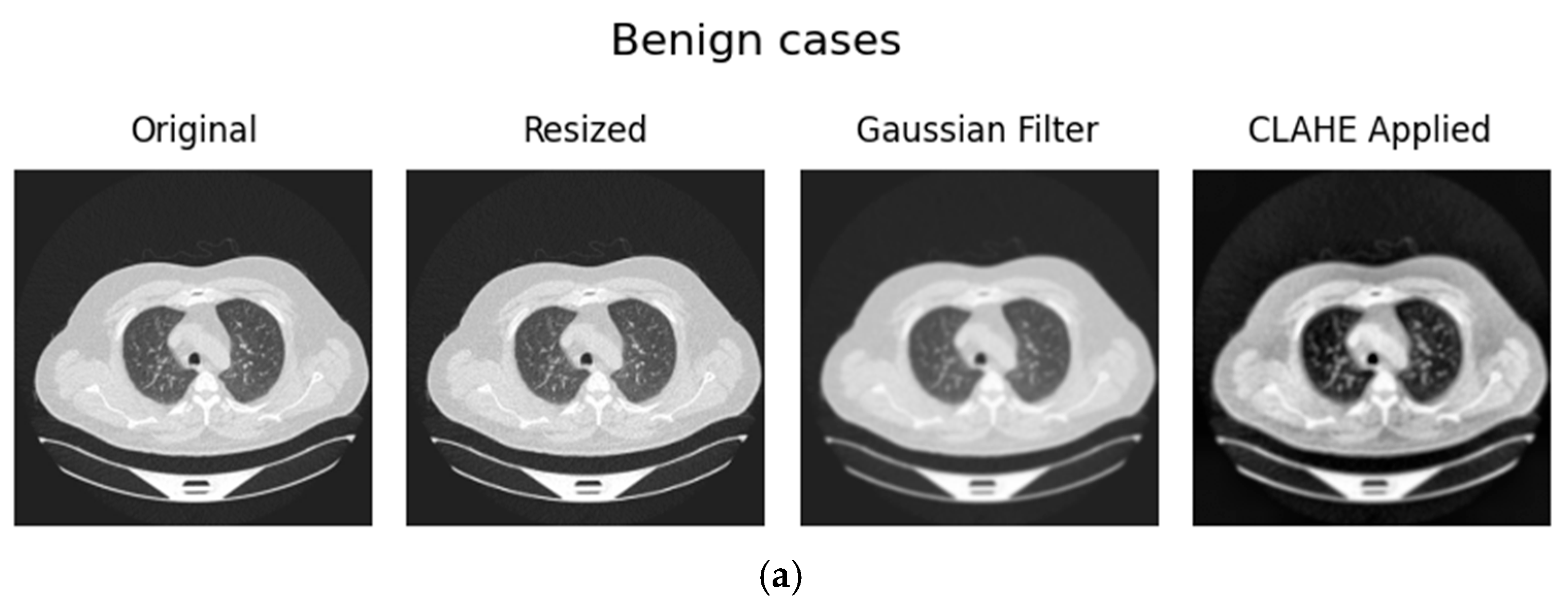
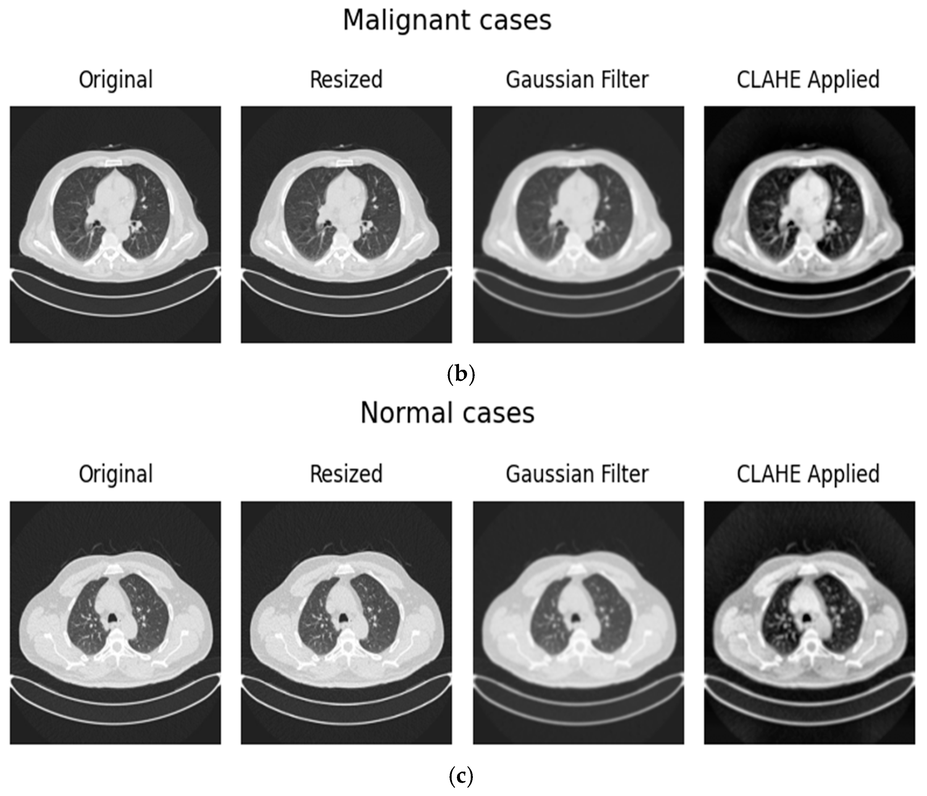
For medical images to be suitable for diagnosis, they must be both high quality and adequately preprocessed. This essential first step involves a standardized pipeline: resizing images (e.g., to 220 × 220 pixels) for uniformity, applying a Gaussian blur to reduce noise and enhance relevant features [34], and converting to grayscale, which simplifies analysis by focusing on intensity changes instead of color.
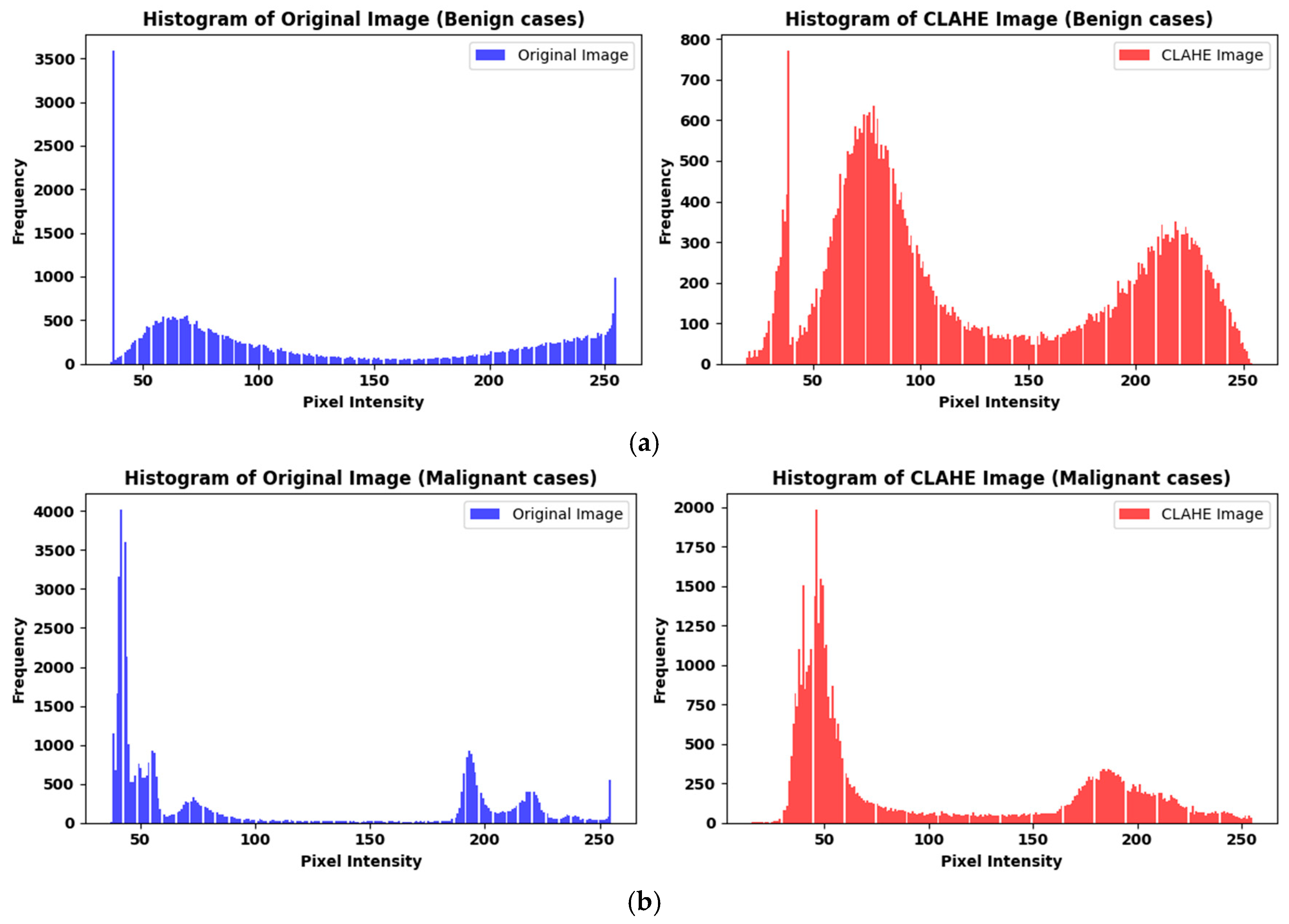
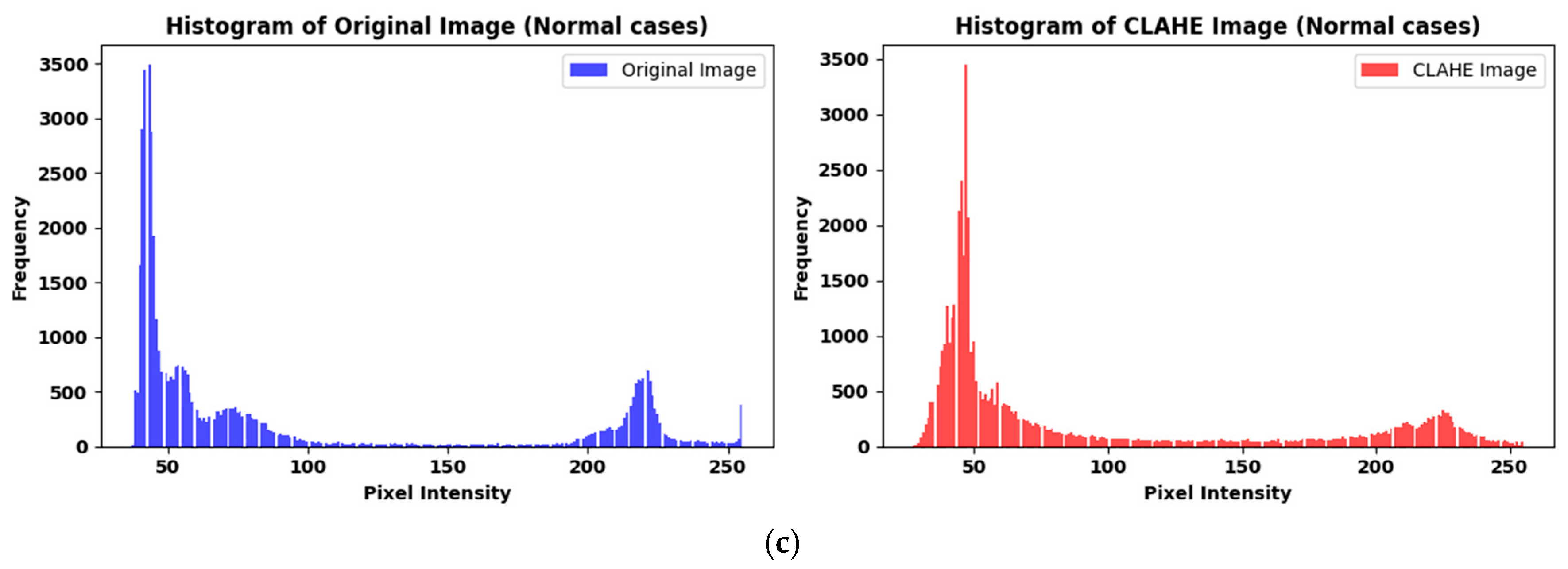
The preprocessing pipeline employs CLAHE (Contrast Limited Adaptive Histogram Equalization) to improve local contrast and accentuate image details by suppressing frequency peaks and redistributing pixel intensities. Subsequently, the input features are standardized to a [0, 1] range by data scaling [37]. As Figure 2 and Figure 3 illustrate, this sequence of operations ensures the images are optimized for subsequent analysis, leading to enhanced accuracy and reliability.

3.1.3. Dataset Split

The dataset was divided into training, validation, and testing subsets, ensuring consistent class distribution across all partitions. A 70:15:15 ratio was applied, resulting in 767 samples for training, 165 samples for validation, and 165 samples for testing. This stratification preserves the class proportions of the original data while supporting balanced learning and unbiased performance assessment.
The training set was used to optimize model parameters, the validation set to fine-tune hyperparameters and monitor overfitting, and the testing set to evaluate the final model’s generalization.

3.1.4. Strategy to Handle Data Imbalance

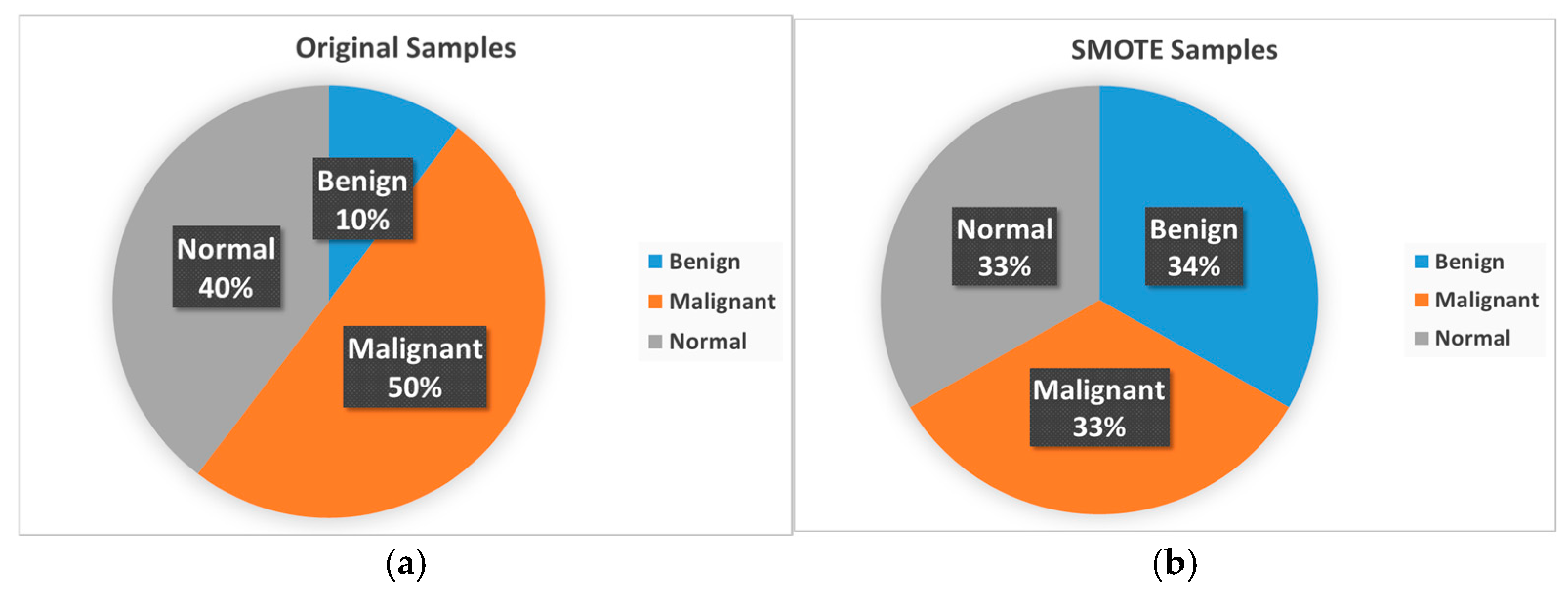
In order to guarantee accurate and dependable machine learning models, it is imperative to address imbalances in datasets, like the IQ-OTH/NCCD lung cancer dataset. Synthetic Minority Oversampling Technique (SMOTE) is a useful method for addressing this problem. In order to balance the dataset and enhance the model’s performance, SMOTE creates synthetic samples for the minority class [38].
The majority class has substantially more samples than the minority class in an unbalanced dataset, which results in biased models that support the majority class. Performance may suffer as a result, particularly when predicting the minority class. SMOTE addresses this issue by using the existing samples to create new, synthetic samples for the minority class. It accomplishes this by identifying its k-nearest neighbors after choosing a sample from the minority class. Following that, it creates new samples along the line segments that connect the chosen sample to its neighbors.
Applying SMOTE makes the dataset more balanced, which helps the model learn better decision boundaries and perform better on the minority class. In medical datasets, precisely identifying uncommon conditions, such as malignant tumors, is beneficial and necessary for patient outcomes. This can be seen in Figure 4 and Table 2.

3.2. Model Architecture and Training Approach

3.2.1. LCxNet Model Implementation

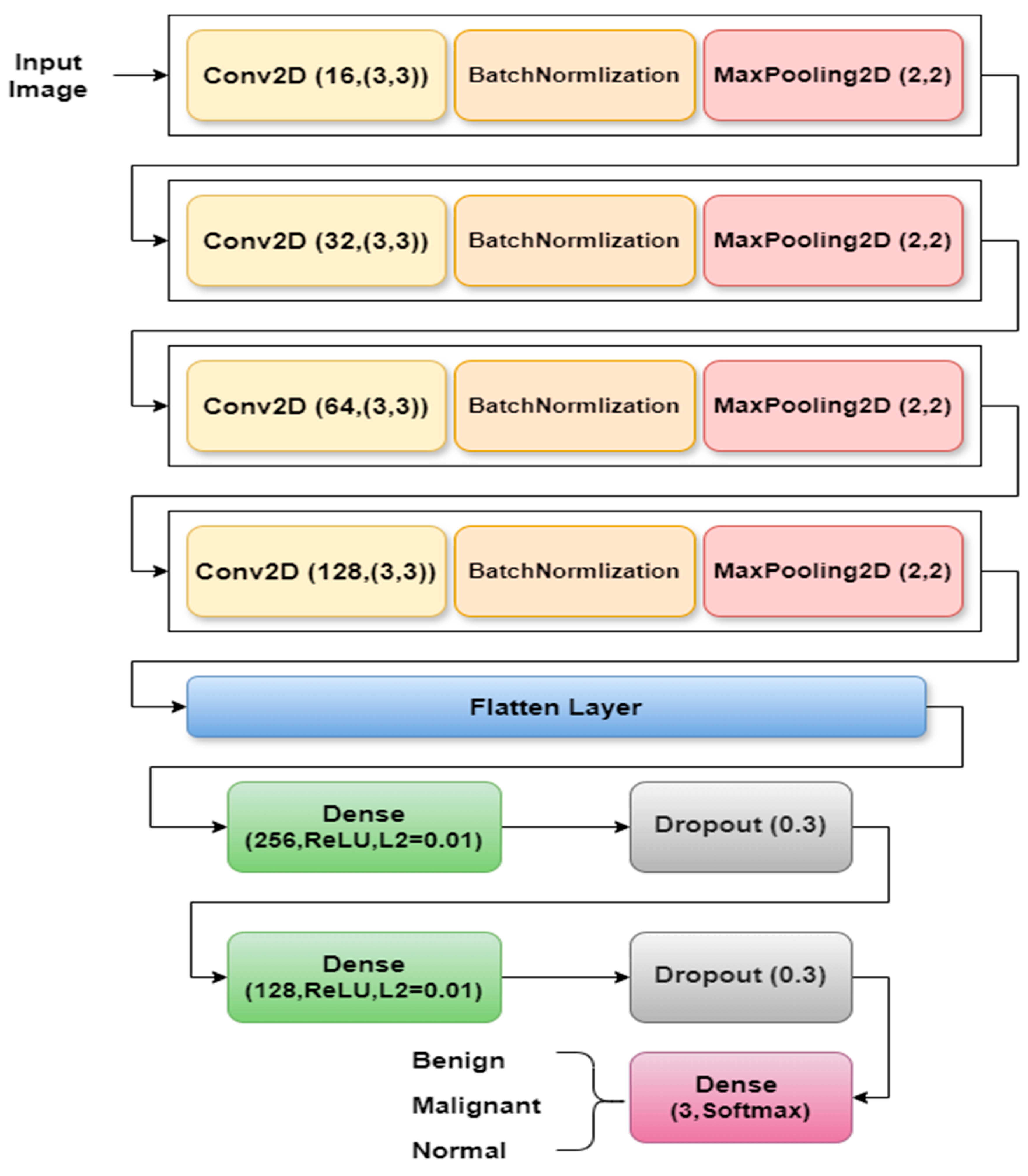
A CNN is a neural network based on the Multilayer Perceptron, enhanced with specialized layers such as convolutional, pooling, and dropout layers [39]. As shown in Table 3, CNN processes 220 × 220 grayscale images (1 channel) through four sequential blocks, followed by dense layers for classification.
The feature extraction process consists of several blocks.
  • Block 1 consists of a 3 × 3 Conv2D layer with 16 filters, producing an output of 218 × 218 × 16 with 160 parameters. Next comes BatchNormalization, which stabilizes activations with 64 parameters, and a 2 × 2 MaxPooling2D layer that reduces the output to 109 × 109 × 16.
  • Block 2 comprises a 3 × 3 Conv2D layer with 32 filters, resulting in an output of 107 × 107 × 32 with 4640 parameters, It is followed by a BatchNormalization layer with 128 parameters, and a MaxPooling2D layer which reduces the output to 53 × 53 × 32.
  • Block 3 features a 3 × 3 Conv2D layer with 64 filters, resulting in an output of 51 × 51 × 64 with 18,496 parameters. BatchNormalization follows this with 256 parameters and a MaxPooling2D layer, which reduces the output to 25 × 25 × 64.
  • Block 4 consists of a 3 × 3 Conv2D layer with 128 filters, generating an output of 23 × 23 × 128 with 73,856 parameters. It also includes BatchNormalization with 512 parameters and a MaxPooling2D layer, which reduces the output to 11 × 11 × 128.
The Flatten layer in the Classification Head first converts the 11 × 11 × 128 output to 15,488 units. The bulk of the network weights are found in the dense layer, which has 256 units with L2 regularization (0.01) to reduce overfitting and 3.9 million parameters. To regularize the network, a dropout layer (0.3) comes after the first dense layer. A second dense layer with 128 units using L2 regularization (0.01) and 32,896 parameters are then added, followed by dropout (0.3). Finally, as indicated in Figure 5, a 3-unit dense layer with 387 parameters is used for the 3-class output.

3.2.2. Optimization Strategy

An important consideration in deep learning model training is the optimizer selection, which has a significant impact on the models’ learning effectiveness, rate of convergence, and performance metrics [40]. Various optimizers employ different approaches to update model parameters, enabling efficient exploration and minimization of the loss landscape. Each optimizer adapts the parameter adjustments based on specific rules, such as learning rates, momentum, or adaptive moment estimates, which influence how the model converges during training.
  • SGD (Stochastic Gradient Descent) with momentum (0.9): By lowering oscillations during training, momentum helps stabilize and speed up convergence, though further fine-tuning may be required for best results. As seen in Equations (1) and (2), where θt are the parameters at iteration t, β is the momentum decay rate (typically 0.9), α is the learning rate, and θ J θ is the gradient of the loss function with respect to parameters ɵ at time step t.
v t = β v t 1 + 1 β θ J θ
θ t + 1 = θ t α v t
  • RMSprop (Root Mean Square Propagation): It is excellent at handling sequential tasks or models that are prone to noisy gradients because it dynamically adjusts learning rates based on recent gradients, guaranteeing steady and reliable updates during training. As shown in Equations (3) and (4), where ϵ a small constant (e.g., 1 × 10⁻⁸) to prevent division by zero.
v t = β v t 1 + ( 1 β ) ( θ J θ ) 2
θ t + 1 = θ t α v t ^ + ϵ θ J θ
  • Adam (Adaptive Moment Estimation): This optimizer is very flexible and effective for a variety of tasks because it combines the advantages of adaptive learning rates and momentum. First moment estimate momentum as indicated in Equation (5), then second moment estimate RMS of gradients as seen in Equation (6).
m t = β 1 m t 1 + 1 β 1 θ J θ
where m t is the exponentially decaying average of past gradients (the first moment), and β 1 is the decay rate for this momentum term (typically 0.9). This term helps accelerate gradient descent in relevant directions by smoothing noisy gradients.
v t = β 2 v t 1 + 1 β 2 ( θ J θ ) 2
Here, v t is the exponentially decaying average of the squared gradients (the second moment), and β 2 is the decay rate for this term (typically 0.999). Captures the variance of the gradients to scale the learning rate adaptively, reducing the step size for parameters with large or noisy gradients. After this, calculate bias-corrected moment estimates as shown in Equations (7) and (8).
m t ^ = m t   / ( 1 β 1 t )
v t ^ = v t   / ( 1 β 2 t )
The parameter update rule then becomes as shown in Equation (9).
θ t + 1 = θ t α v t ^ + ϵ m t ^
  • AdamW (Adaptive Moment Estimation with Weight Decay): By incorporating decoupled weight decay regularization, this enhanced Adam optimizer successfully improves generalization and reduces overfitting [41]. Equations (5)–(8) are used, and the parameters are updated by subtracting the adaptive gradient step and a scaled weight decay term, as seen in Equation (10).
θ t + 1 = θ t α ( m t ^ v t ^ + ϵ + λ θ t )
  • NAdam (Nesterov-accelerated Adaptive Moment Estimation): Combines the adaptive moment estimation of Adam with Nesterov accelerated gradients (NAG), which introduces a “lookahead” gradient step to improve convergence speed and stability [42]. Unlike Adam, which uses the current gradient to update parameters, NAdam incorporates the gradient at the anticipated next position, effectively providing a more responsive momentum update. v t , v t ^ remain the same as in Adam Equations (6) and (8). However, the parameter update utilizes a lookahead gradient estimate, as seen in Equation (11).
  m t   ^ N A d a m = β 1 m t ^ + ( 1 β 1 ) θ J θ
The parameter update rule thus becomes Equation (12).
θ t + 1 = θ t v t ^ + ϵ   m t   ^ N A d a m

3.2.3. The t-SNE Visualization

t-distributed Stochastic Neighbor Embedding (t-SNE) is an unsupervised ML method that emphasizes non-linear dimensionality reduction [40]. By maintaining the local structure of the data, it transforms high-dimensional data into interpretable 2D or 3D embeddings. To achieve this, pairwise similarities between data points are modeled in both the original and embedded spaces. The mapping is then optimized to reduce the divergence between these similarity distributions. Finding meaningful clusters and patterns in complicated datasets is made easier with the help of this kind of visualization. Because it reveals underlying structures that enhance dataset comprehension and inform decision-making in subsequent training procedures, t-SNE is particularly beneficial for preprocessing CT images before training CNNs [43].

3.2.4. Explainable Artificial Intelligence (XAI) Techniques

The CNNs are frequently referred to as “black-box” algorithms because it is challenging to comprehend their complex decision-making procedures. This lack of transparency has become a major obstacle that prevents CNNs from being effectively applied to a variety of real-world issues. This problem is addressed by XAI, which focuses on making DL models understandable and intuitive [44]. By bridging the gap between sophisticated algorithms and human comprehension, XAI seeks to make decision-making processes both accessible and understandable to users. Grad-CAM is used for XAI interpretation; it was first introduced in 2017. Highlights areas that affect a CNN’s decision by creating heatmaps using gradients from a target class flowing into particular convolutional layers [45]. Here is a detailed mathematical implementation [46]:
  • Compute Gradients: Calculate the gradients of the target class score Y c with respect to the feature map A k of a specific convolutional layer, as shown in Equation (13).
    Y c A i j k
    where A i j k is the activation at spatial location (i,j) in the k-th feature map.
  • Global Average Pooling (GAP) for Weights: Compute the neuron importance weights k c for each feature map k as shown in Equation (14). This is achieved by performing a global average pool of the gradients calculated in step 1.
    k c = 1 Z   i j Y c A i j k
    where Z is the total number of spatial locations (i.e., Z = u x v ), these weights represent the “importance” of feature map k for the target class c.
  • Weighted Sum of Feature Maps: Compute the ReLU-activated weighted sum of the feature maps using the calculated weights k c . Produces the raw Grad-CAM heatmap L G r a d C A M c as illustrated in Equation (15).
    L G r a d C A M = R e L U ( k k c A k ) c
    The ReLU is applied because we are typically interested in features that positively influence the class score.
  • Upsampling and Superimposition: The resulting heatmap L G r a d C A M c is typically low-resolution (same as the feature map). It is then upsampled to the original input image size and superimposed onto the input image to visualize the regions of interest that most influenced the CNN’s decision for the target class. These visualizations appear as “heatmaps.”

4. Experimental Results

4.1. Performance Metrics

When evaluating a classification model, it is crucial to consider several key metrics that provide insights into its performance and effectiveness [13]. An essential tool for assessing classification models is a confusion matrix, which displays the numbers of false positives (FP), false negatives (FN), true positives (TP), and true negatives (TN), to provide an overview of how well the model predicts each class. Understanding metrics such as accuracy, precision, recall, F1-score, and ROC-AUC is vital for assessing a classification model’s actual performance. Each metric provides a distinct perspective on the model’s performance, facilitating a comprehensive evaluation. Equations (16) to (21) are provided in Ref. [28].
Accuracy: calculates the proportion of correctly predicted occurrences (TP and TN) out of every case to determine the model’s overall accuracy. It works best when the dataset is balanced and the costs of false positives and false negatives are comparable. Equation (16) can represent it.
A c c u r a c y = T P + T N T P + T N + F P + F N
Precision: also referred to as the positive predictive value, it shows the percentage of actual positive predictions among all of the model’s positive predictions. Equation (17) can represent it.
P r e c i s i o n = T P T P + F P
Sensitivity (Recall or True Positive Rate (TPR)): calculates the percentage of true positives among all actual positives that the model correctly detects. Equation (18) can represent it.
S e n s i t i v i t y ( R e c a l l ) = T P T P + F N
F1-score: as shown in Equation (19), it takes the harmonic mean of precision and recall to find a balance between the two. Particularly helpful when working with unbalanced datasets or when balancing precision and recall.
F 1 - S c o r e = 2 P r e c i s i o n     R e c a l l P r e c i s i o n + R e c a l l
Specificity (True Negative Rate (TNR)): as shown in Equation (20), measures the proportion of actual negative cases correctly identified by the model. It evaluates the model’s ability to avoid false positives.
S p e c i f i c i t y = T N T N + F P
Cohen’s Kappa is a statistical metric used to assess the agreement between two raters or classifiers while controlling for chance agreement [28]. It is beneficial when dealing with imbalanced classes. Equation (21) can represent it.
C o h e n s   K a p p a = A c c u r a c y R a n d o m   A c u u r a c y 1 R a n d o m   A c u u r a c y
Receiver Operating Characteristic—Area Under the Curve (ROC-AUC): measures the area under the ROC curve, which plots the True Positive Rate (TPR) against the False Positive Rate (FPR) across all classification thresholds [29]. As represented in Equations (22) and (23).
F P R = F P F P + F N
A U C = 0 1 T P R t d F R P t
Precision-Recall Curve (PR): The PR curve plots precision (y-axis) against recall (x-axis) for various thresholds [47]. The area sums up the model’s precision-recall trade-off under this curve (PR-AUC). Equation (24) can represent it.
P R A U C = 0 1 P r e c i s i o n ( R e c a l l )   d ( R e c a l l )
Misclassification Rate (MR): provides the proportion of incorrect predictions out of all predictions [22] as shown in Equation (25).
M i s c l a s s i f i c a t i o n   R a t e   M R = 100 A c c u r a c y

4.2. Hyperparameters Configuration

To achieve optimal performance, strength, and generalization potential, it is essential to rely on the adjustment of hyperparameters [48]. The image size (220 × 220 × 1) is one of the crucial parameters that affects feature extraction quality by dictating input resolution; larger sizes can increase accuracy but also raise computational costs. A balance between training stability and computational efficiency is maintained by using a batch size of 16, with smaller sizes possibly resulting in slower training but better generalization. The optimizer’s initial learning rate of 0.001 was chosen to ensure controlled and stable updates, thereby avoiding divergence. A total of 35 training epochs was used to maintain a balance between underfitting and overfitting, with early stopping applied to terminate training once the validation performance plateaued. Fine-tuning these hyperparameters is crucial for enhancing the robustness, precision, and clinical reliability of CNNs. Table 4 details the specific configurations adopted in this study.

4.3. Experimental Setup

The study used state-of-the-art hardware and software tools to ensure optimal performance and conduct computational experiments. The experiment was conducted using Google Colab Pro. This programming environment included Python 3.10.12 and Windows 10, as well as well-known libraries such as Keras and TensorFlow for constructing and training CNN models.

4.4. Optimization Analysis

4.4.1. The Weight Decay’s Effect on AdamW

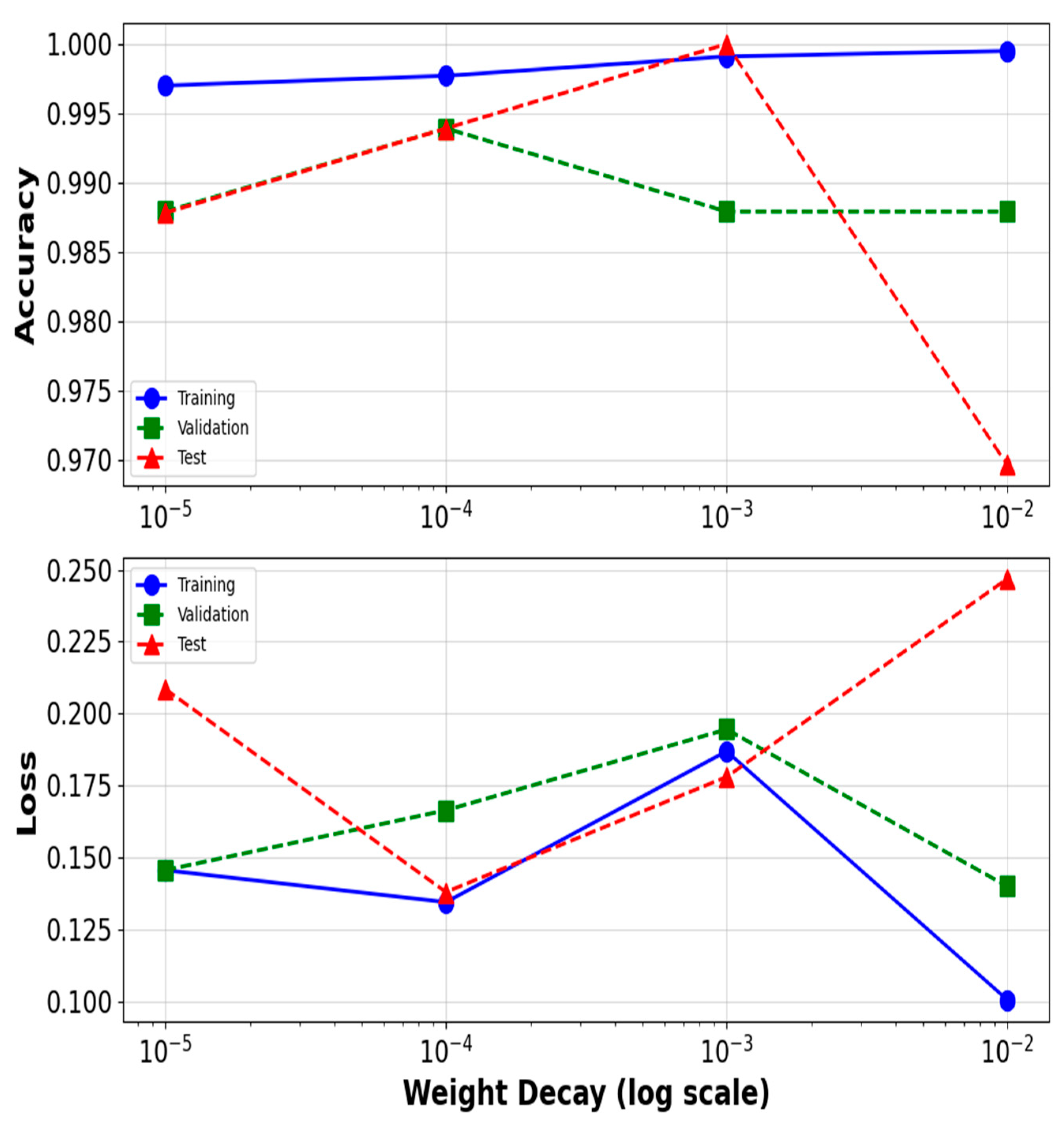
To find the ideal weight decay for AdamW in CT scan analysis, four weight decay values [1 × 10⁻⁵, 1 × 10⁻⁴, 1 × 10⁻³, 1 × 10⁻²] are evaluated, where reducing false negatives and positives is crucial.
The results show that 1 × 10⁻⁴ yields the most dependable results. It offers the best trade-off between validation accuracy and test accuracy, as well as loss. This choice avoids overfitting, as seen with 1 × 10⁻³, which achieves perfect test accuracy but shows unstable validation performance, and prevents underfitting, as observed with 1 × 10⁻², which sacrifices accuracy for loss reduction. Thus, 1 × 10⁻⁴ ensures robust generalization and stable validation performance. This is illustrated in Figure 6.

4.4.2. The Optimizer’s Effect on Model Performance

The choice of optimizer has a significant impact on a model’s ability to classify lung nodules from CT accurate scans into benign, malignant, or normal categories. From Table 5, we can analyze how each optimizer’s performance metrics translate to clinical relevance in this high-stakes medical domain. Weighted metrics provide a more reliable evaluation than macro or micro averages for imbalanced multiclass data, ensuring all class performances contribute proportionally to the evaluation [49].
The Adam-family optimizers (Adam, AdamW, NAdam) outperform SGD and RMSprop in overall accuracy, precision, and the crucial balance of precision and sensitivity.
Specifically, AdamW emerges as the most suitable optimizer for this lung cancer classification task. Its unparalleled sensitivity of 99.39% is paramount, ensuring that the risk of missing a malignant tumor (false negative) is minimized, which is a top priority in clinical diagnostics. Coupled with its high accuracy (99.39%), precision (99.40%), F1-score (99.40%), and low generalization loss (0.17), AdamW offers the most robust and clinically reliable performance for aiding in the early and accurate detection of lung cancer.
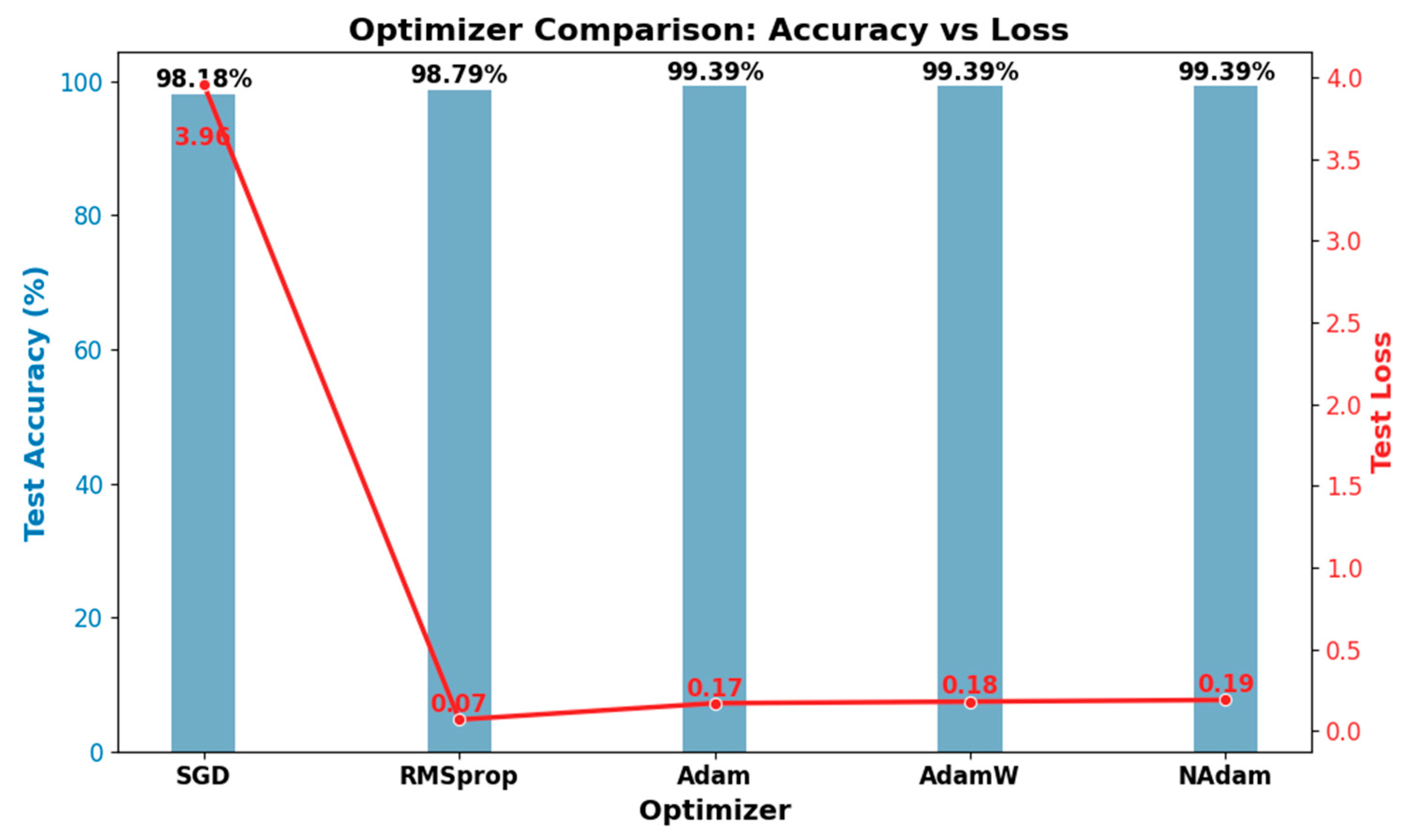
While Adam and NAdam are also excellent choices, AdamW’s slight edge in specificity (99.89%) and Cohen’s Kappa (99.01%) provides a meaningful clinical advantage by reducing false positives and improving overall diagnostic agreement. Although RMSprop achieves a low loss, both it and SGD perform worse in the key metrics, rendering them less optimal for this medical application. The results shown in Figure 7 indicate that while SGD starts with high loss, optimizers like Adam and NAdam achieve high accuracy with significantly reduced loss.

4.4.3. Training Performance and Convergence Analysis

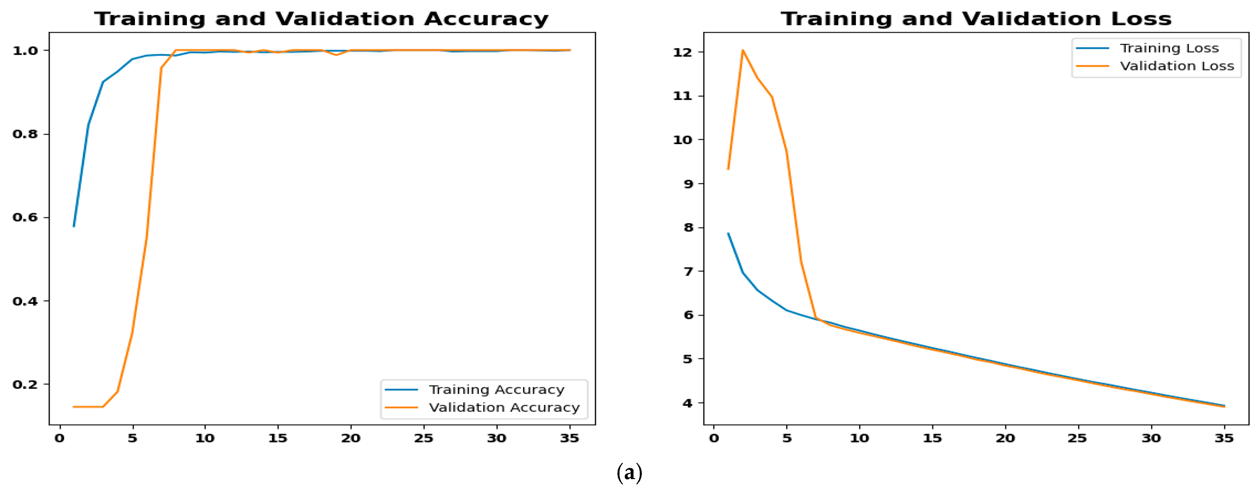
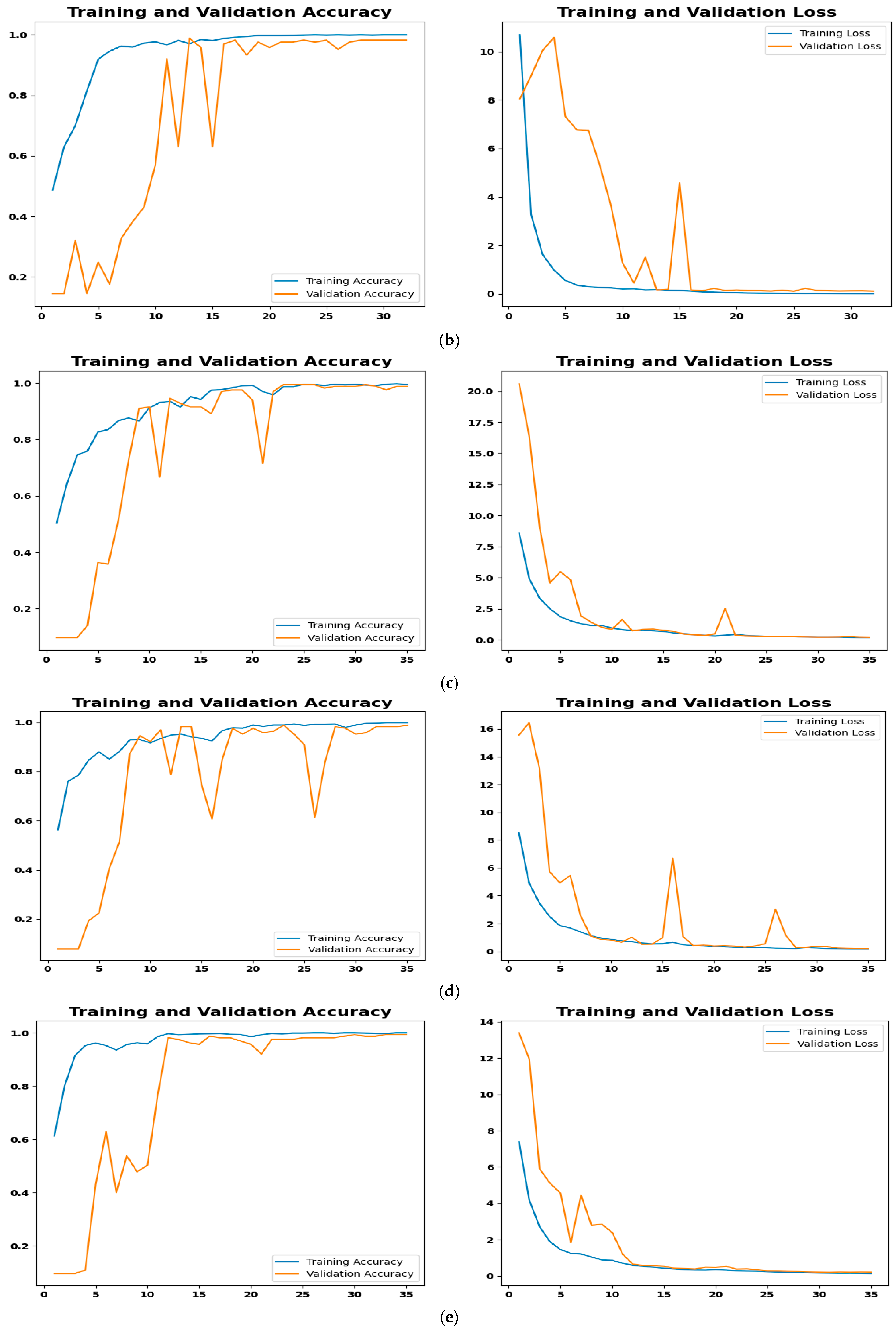
The LCxNet model was trained over 35 epochs using 70% of the dataset. As demonstrated in Figure 8, over epochs, training and validation accuracy gradually increase, while training loss and validation loss steadily decrease. To prevent overfitting, early stopping was implemented, which halted training when the validation performance stopped improving. This strategic approach ensured that the model did not become overly specialized to the training data.

4.4.4. Model Evaluation Metrics

The 165 test cases, which include benign, malignant, and normal lung conditions, give an overview of how well each optimizer supports the model’s performance in a practical diagnostic setting. The main objective of lung cancer screening and diagnosis is to reduce the possibility of overlooking malignant cancer cases while simultaneously minimizing needless procedures or anxiety for patients with benign conditions or healthy lungs.
  • Figure 9a: Although it has a minor flaw in handling benign cases, the SGD optimizer’s confusion matrix correctly identified 162 out of 165 cases. The misclassification rate was only 1.82%, with two cases being incorrectly classified as malignant and one as normal. This is less serious than missing a real cancer because it may make patients anxious, necessitate invasive diagnostic procedures, and result in needless medical expenses.
  • Figure 9b: The model performs marginally better with RMSprop; only two benign cases, both of which were misclassified as normal. This indicates that RMSprop does not make the vital mistake of generating false positives for malignant cases, unlike SGD, which demonstrated this issue with benign cases. A positive result in the clinical setting of lung cancer since it lessens the possibility of needless procedures based on a benign finding. Without such misunderstandings, the model shows excellent accuracy in distinguishing between malignant and normal cases. The rate of misclassification is 1.21.
  • Figure 9c: With only 1 out of 165 cases misclassified, the Adam optimizer has a high overall accuracy rate, suggesting a strong model. One malignant case, however, was mistakenly identified as normal, which raises concerns in medical diagnostics. A poorer prognosis, delayed treatment, and disease progression could result from a missed diagnosis. The numerical advantage in accuracy for patient safety is outweighed by the misclassification rate of 0.61.
  • Figure 9d: With just one case misclassified—a normal case that was classified incorrectly as benign—AdamW has a high overall accuracy rate. AdamW is a safer option for situations requiring few false negatives for malignancy because it avoids missing a serious cancerous condition, which makes it less severe than Adam’s misclassification.
  • Figure 9e: NAdam, a model similar to Adam and AdamW, achieves high accuracy with only one misclassification. It achieves 100% recall for malignant cases, a significant advantage over Adam, which had one critical false negative. The single misclassification in NAdam is a benign case being missed and called normal, which is less essential in lung cancer diagnosis.
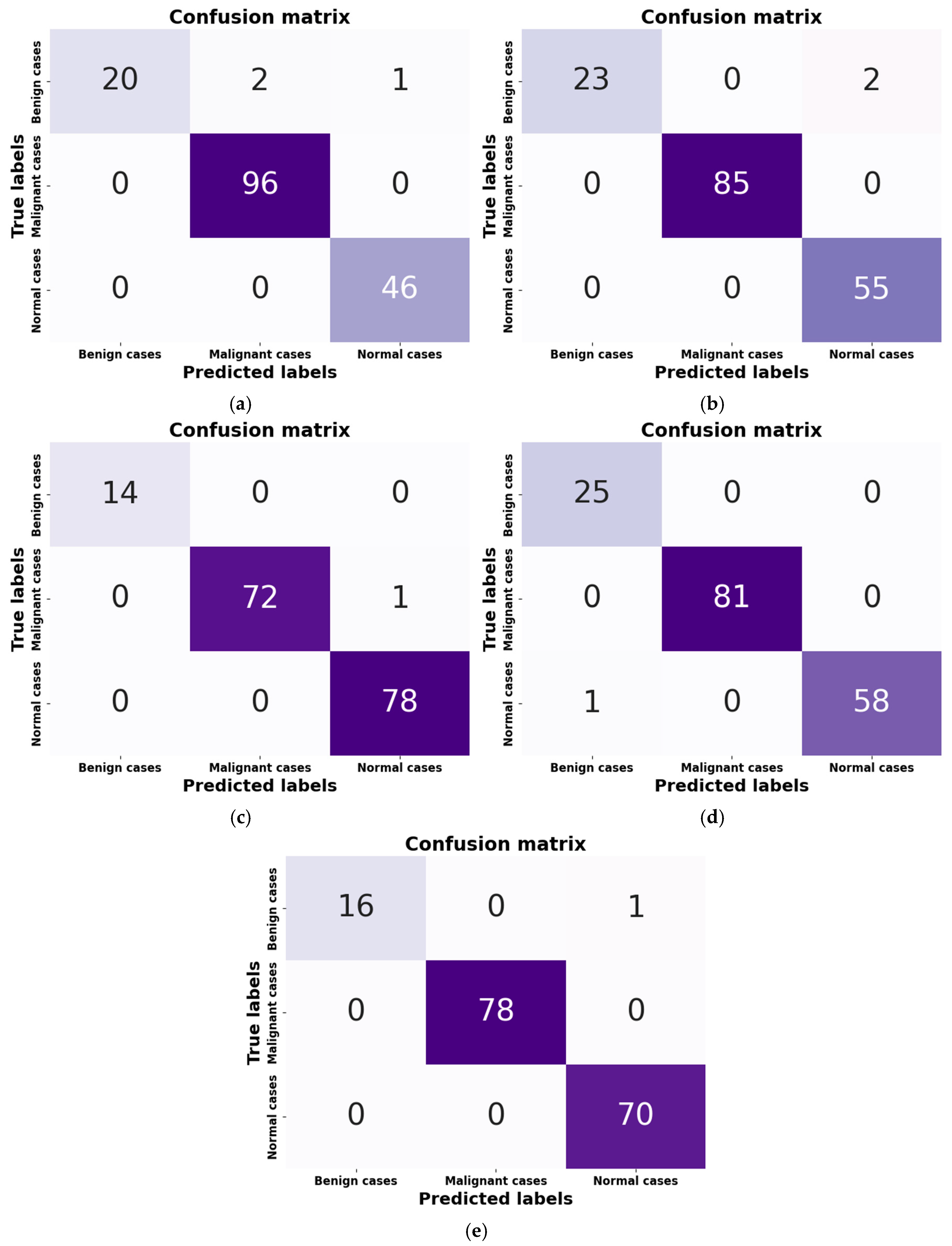
Though SGD introduces false positives for malignant cases, which could result in over-investigation, RMSprop and SGD are generally good. The Adam family optimizers, Adam, AdamW, and NAdam, have a similar numerical misclassification rate of 0.61% in lung cancer diagnostic scenarios. However, AdamW and NAdam are clinically safer due to their ability to avoid missing malignant cases.
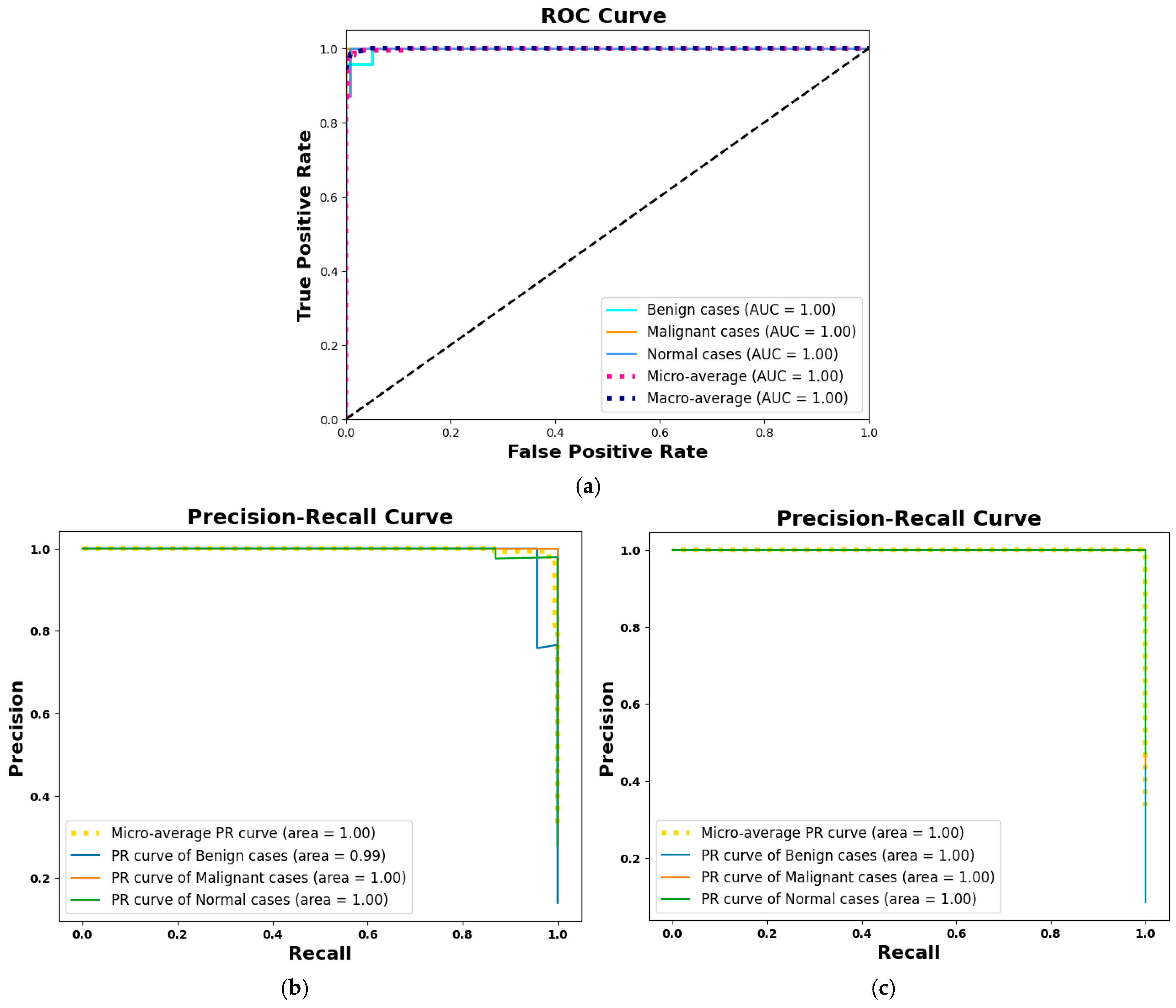
Figure 10 display the ROC-AUC and PR plots, respectively. These plots provide an evaluation of the model’s performance, highlighting its ability to distinguish between classes and handle imbalanced datasets effectively.
Figure 9. Confusion matrix. (a) SGD, (b) RMSprop, (c) Adam, (d) AdamW, (e) NAdam.
Asi 08 00153 g009
Figure 10. (a) The ROC curve shows outstanding performance, with the model achieving a perfect AUC score of 1.00 across all classes (all optimizers achieve the same results). (b) The PR curve highlights performance for SGD and RMSProp optimizers. (c) The PR curve for the Adam family of optimizers is shown.
Asi 08 00153 g010

4.5. Visualization of High-Dimensional Data Structure Using t-SNE

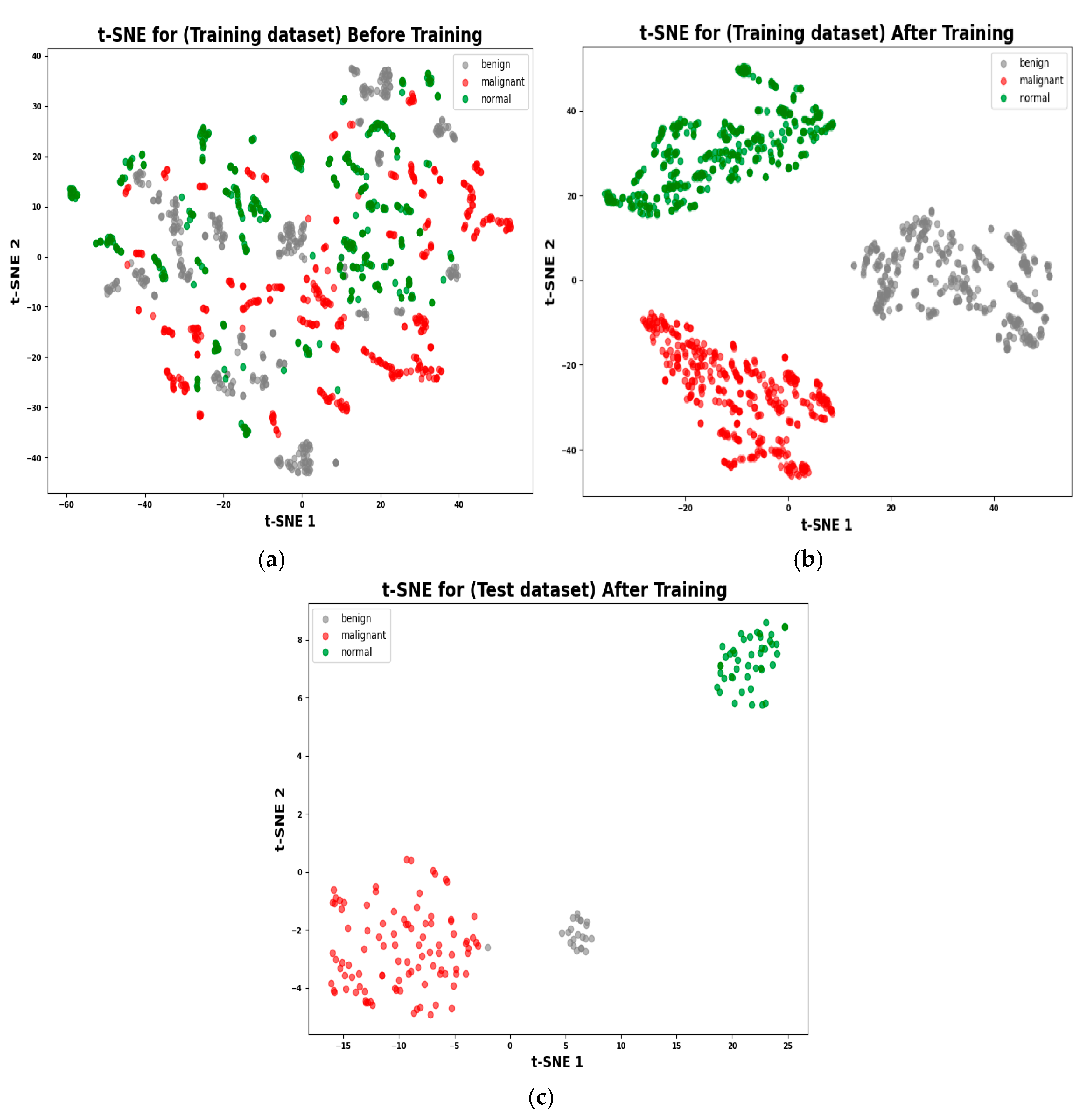
Figure 11a shows that the t-SNE visualization reveals the classes are not easily distinguishable, forming intricate and challenging-to-separate clusters. Illustrates the inherent complexity and high dimensionality of the original data, which hinders the straightforward application of linear models in producing accurate classifications. The visualization underscores the need for learning more discriminative features, which necessitates a more sophisticated model architecture, such as a convolutional neural network (CNN).
Figure 11b shows that the LCxNet model has effectively learned highly abstract and discriminative features during its training process, as this visualization effectively illustrates. To make accurate classification within the training data, it has converted the complicated, overlapping input features into a new representation where the various lung conditions are much more linearly separable.
Figure 11c shows that the LCxNet model exhibits a clear separation of clusters in the test dataset, indicating robust feature learning and enabling high accuracy and reliable performance in real-world cases. This separation of unseen data points from different classes allows for confident classification of new samples into lung condition categories.

4.6. Interpretation of CNN Decisions Using Grad-CAM Heatmaps

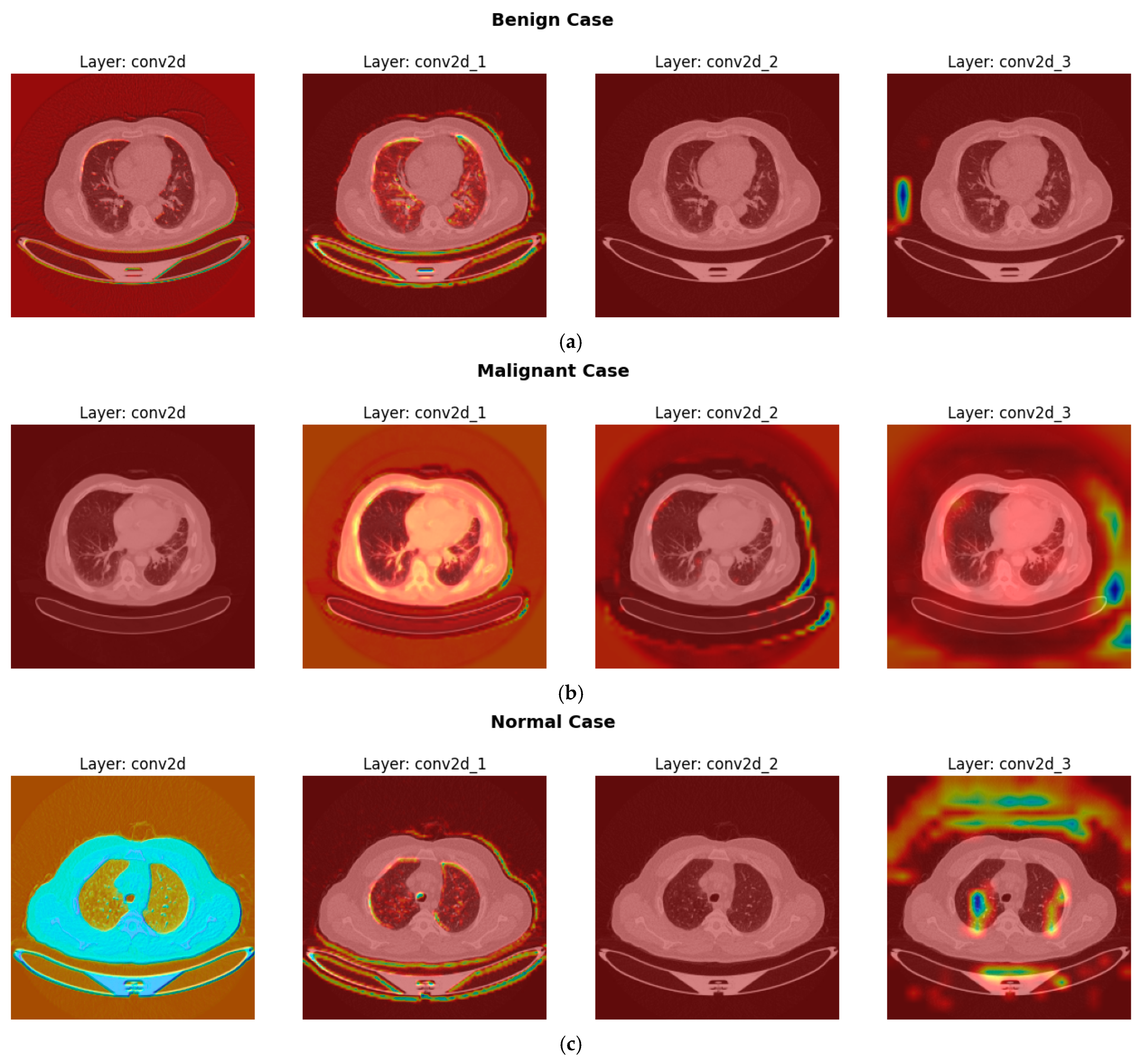
Although the original approach mainly concentrates on the last convolutional layer because it has spatial information and preserves high-level semantic information, examining several layers offers a more thorough understanding of hierarchical feature learning. As seen in Figure 12, the Grad-CAM visualizations for every class display various layers. The foundation of the input data is formed by early layers (such as conv2d), which capture fundamental features like edges and textures. By combining these fundamental characteristics, mid layers (e.g., conv2d_1, conv2d_2) can recognize intermediate-level structures and identify more intricate patterns. High-level semantic and class-specific features that directly affect the model’s decisions are encoded in the final layer (e.g., conv2d_3).

4.7. Ablation Study

4.7.1. Impact of Data Split Ratios on Model Performance

The split ratio has a significant impact on the capacity of deep learning models to identify patterns in the training set and generalize to new data. Selecting the optimal ratio is necessary to maintain accurate performance metrics while striking a balance between underfitting and overfitting.
  • The 70:15:15 split offers a well-balanced training and evaluation strategy, making it ideal for achieving high accuracy and strong generalization capabilities.
  • The 80:10:10 split enhances sensitivity and improves the detection of positive cases by increasing the size of the training set. However, because there is less validation data available for hyperparameter tuning, overall performance is somewhat decreased.
  • The 80:20 split reduces the amount of validation and testing data, potentially limiting the model’s generalization capabilities. In this case, validation constitutes 20% of the training set, which means 16% of the original dataset.
The 70:15:15 and 80:10:10 ratio splits yielded the best results, as shown in Table 6. In contrast, the 80:20 configuration yielded the poorest performance because it utilized a validation set derived from the training data. This draws attention to the importance of using independently chosen validation sets for reliable model testing and tuning.

4.7.2. Impact of Dataset Size on Model Performance

The IQ-OTH/NCCD dataset shows difficulties because of its unbalanced class distribution and small size. To solve this, Kaggle data augmentation methods were used to artificially increase the dataset by about ten times [50]. Then, using stratified sampling to maintain class distributions, the augmented dataset was divided into 80:20 training and testing sets. Class weighting was used during training to further reduce class imbalance by giving minority classes heavier penalties. Without changing the model’s basic prediction mechanism, this method enhanced the model’s predictive performance on underrepresented classes.
To achieve robust generalization, an LCxNet was trained utilizing five optimizers, each with a learning rate of 1 × 10⁻³ AdamW, configured with a weight decay of 1 × 10⁻⁴, was determined to be optimal, effectively balancing validation and test accuracy and loss, and mitigating overfitting and underfitting.
According to Table 7, AdamW is the best optimizer for this dataset because it provides the best possible balance between excellent error minimization, strong overall metrics, and high accuracy. Even though Adam does exceptionally well, AdamW is the better option for this particular classification task due to its slight improvements overall, especially in obtaining the lowest test loss and MR.
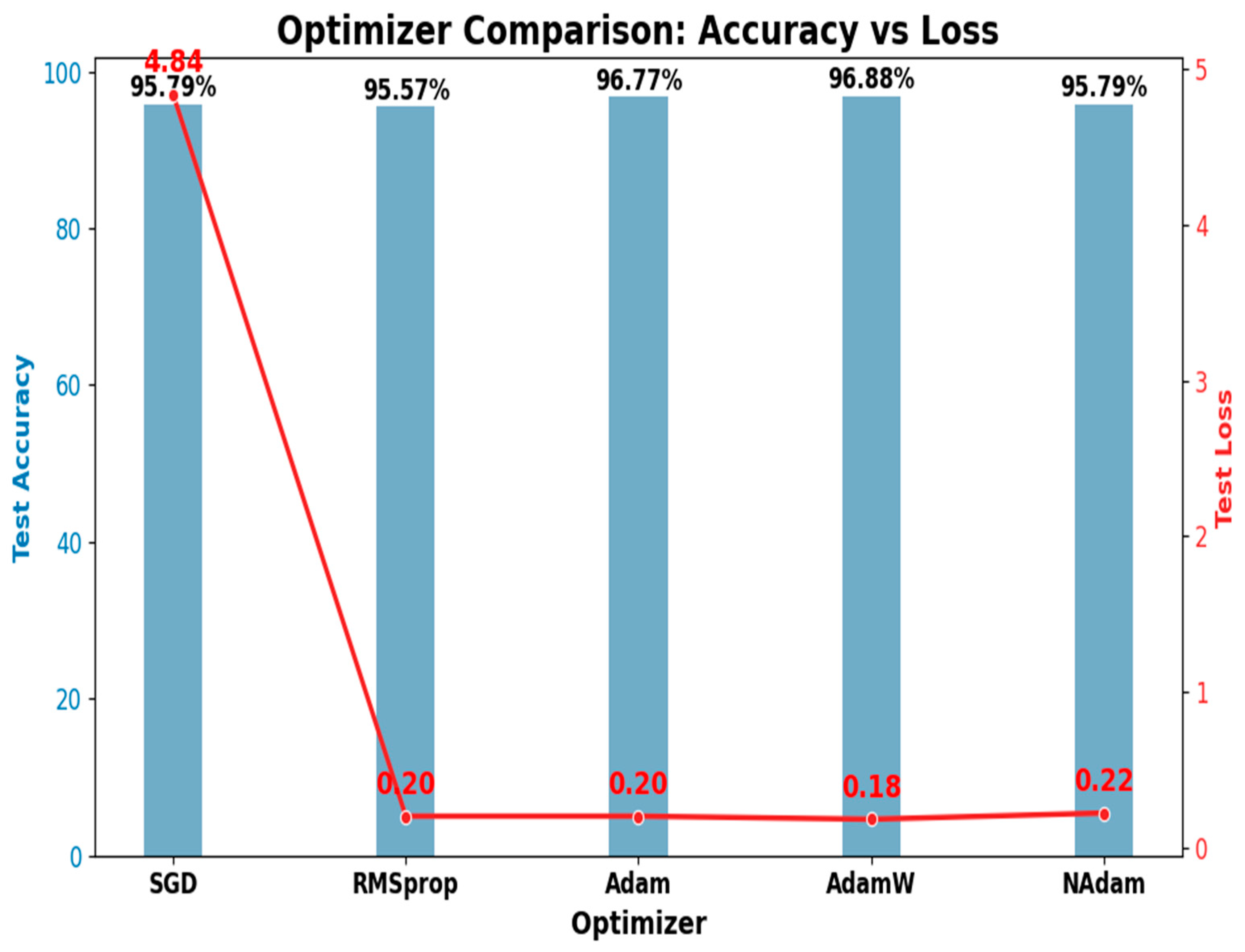
The study also emphasizes the significance of assessing a wide range of metrics, showing that a low-test loss (such as RMSprop’s) does not always imply good classification performance. The optimizer comparison, depicted in Figure 13, reveals interesting trends regarding model performance.
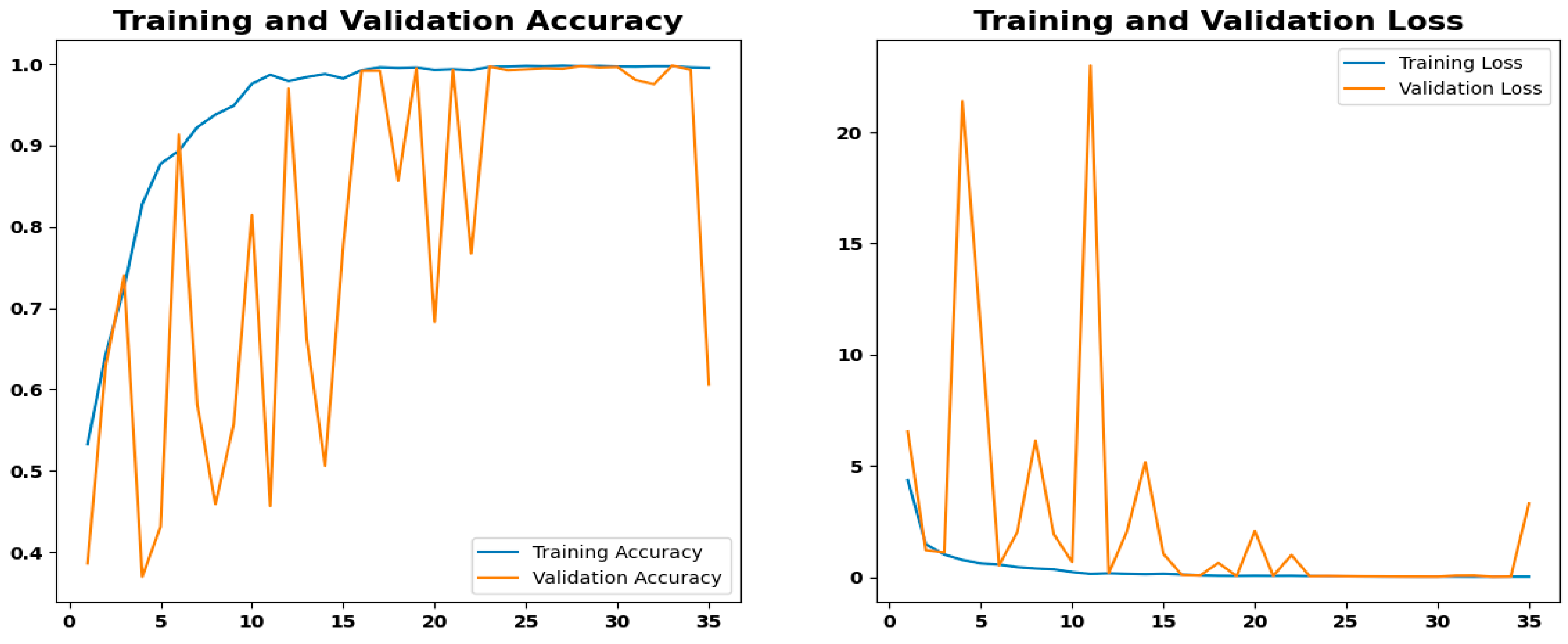
Notably, as illustrated in Figure 14, the model exhibits low loss and high accuracy during training. However, initial variations in the validation metrics point to problems with the model’s generalizability. This behavior may indicate a feedback problem, which could lead to similar performance during training and inflated evaluation results, as the validation and augmented training data originate from the same source. These results underscore the importance of maintaining an objective model evaluation with clinical relevance in mind and dividing participants into discrete groups.

4.7.3. Impact of Modality Type: CT Scans vs. Histopathological Images

The LCxNet model is trained and evaluated using the LC25000 dataset, which emphasizes the distinctions between CT and histopathology as well as the impact of modality type on classification accuracy and generalization [51].
The model’s performance is validated in this study, which also offers insights into multi-modal integration for increased diagnostic accuracy. Three classes for lung cancer (lung adenocarcinoma, lung squamous cell carcinoma, and benign lung tissue) and two classes for colon cancer make up the LC25000 dataset, which consists of 25,000 histopathological images with a resolution of 768 × 768 pixels each. For this study, we only used the lung cancer subset, which consists of 15,000 images evenly distributed across the three classes (approximately 5000 images per class). This well-balanced subset enables efficient and consistent training and evaluation of the model, ensuring stable performance and strong learning outcomes [47].
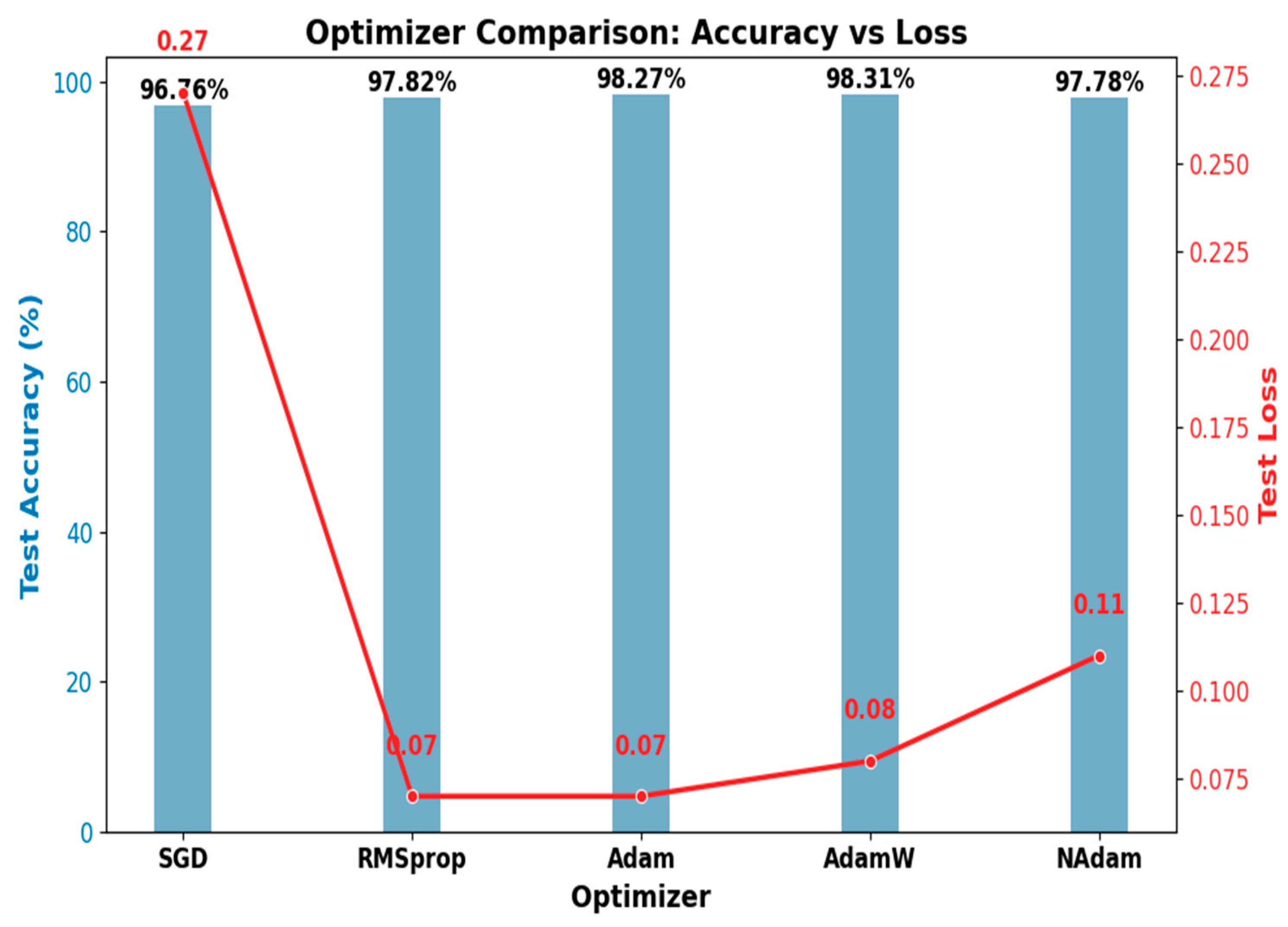
As shown in Table 8, the model’s performance was significantly impacted by the optimizer selection; AdamW performed the best, achieving the highest accuracy of 98.31%. AdamW’s robustness and predictive power were further demonstrated by its superior scores in weighted precision, F1-score, sensitivity, and Cohen’s Kappa. Adam had a marginally smaller loss but performed similarly on all of these measures. With 97.82% accuracy and minimal loss, RMSprop performed well, whereas NAdam displayed marginally worse accuracy and greater loss. With an accuracy of 96.75% and the highest loss of 0.26, SGD performed the worst overall, as would be expected for more complex models. A detailed breakdown of optimizer performance in terms of accuracy and loss can be found in Figure 15.

5. Discussion

5.1. Performance Comparison with TL Models

Transfer learning is an ML technique where knowledge obtained from one task is reused to improve performance on a related task. Instead of training a model from scratch, transfer learning leverages pre-trained models, significantly reducing computational requirements and data needs [52]. This approach is particularly effective in deep learning, where large datasets and extensive training are often required. Models such as VGG16, ResNet50, MobileNetV2, InceptionV3, DenseNet121, and Xception are pre-trained on large datasets like ImageNet by freezing the initial layers and fine-tuning the dense layers, as shown in Table 9.
The LCxNet model accomplishes superior performance with fewer parameters than most traditional architectures, suggesting computational and memory efficiency in addition to accuracy. MobileNetV2’s impressive efficiency and strong metric performance make it ideal for resource-constrained deployment, even if it slightly trails in class-wise granularity.
DenseNet121 achieves a strong overall balance of accuracy, sensitivity, specificity, and F1-score, outperforming most baselines except MobileNetV2 and LCxNet.
Despite its architectural depth, InceptionV3 consistently underperforms across all evaluation metrics, suggesting inadequate generalization to the target dataset.
ResNet50 exhibits good sensitivity and precision but its comparatively low F1-score may indicate that the harmonic mean is being impacted by class imbalance. Both VGG16 and Xception offer robust sensitivity, but lag slightly in balanced prediction (F1-score) and efficiency.
As indicated in Table 9, although MobileNetV2, DenseNet121, and Xception exhibit lower loss values compared to LCxNet, their overall classification performance is inferior. This outcome highlights a key insight: loss value alone is not a definitive indicator of model effectiveness. Although models may exhibit minimal training or validation loss, they may perform poorly in terms of accuracy, sensitivity, and specificity. This is frequently the result of overfitting, inadequate feature extraction, or inadequate generalization to the lung CT dataset utilized in this investigation.
Pre-trained networks like MobileNetV2, DenseNet121, and Xception are primarily tuned for large-scale datasets such as ImageNet. However, without proper fine-tuning or adaptation, these architectures may struggle to generalize in specialized medical imaging tasks. In contrast, LCxNet was explicitly developed for lung cancer classification, tailored to extract clinically relevant features more effectively. Its superior classification performance, despite a higher loss value, underscores the advantage of task-specific design in medical imaging applications.

5.2. Performance Comparison with Other Studies on the IQ-OTH/NCCD

Several significant trends and insights into model architectures, imbalance handling strategies, explainability techniques, and performance metrics are revealed by comparing recent studies on lung cancer classification. Using different CNN architectures and transfer learning models, the majority of previous works concentrate on binary or three-class classification tasks. In Table 10, Abdollahi [53] and Abunajm et al. [54], have shown the effectiveness of data augmentation in addressing the class imbalance, achieving high accuracy levels of 97.88% and 99.45%, respectively.
On the other hand, SMOTE and other oversampling techniques have also been effectively applied by Musthafa et al. [38] and Ganguly and Chakraborty [55], achieving classification accuracies exceeding 99%. These findings highlight the crucial role of imbalance handling in enhancing model performance, particularly for complex tasks like multi-class lung cancer classification. However, oversampling can introduce noise and artificial patterns into the dataset, which may affect model robustness.
Even though there is an increasing focus on XAI, only a handful of studies, such as Raza et al. [56] and Klangbunrueang et al. [47], utilize Grad-CAM to visualize model reasoning. While Grad-CAM enhances transparency, its heatmaps can be ambiguous, sometimes diffusing across broad, non-discriminative regions. This variability necessitates expert interpretation and underscores the importance of pairing visual insights with robust quantitative metrics for clinically meaningful validation.
In this paper, the suggested LCxNet model incorporates Grad-CAM for interpretability and SMOTE for balancing, integration of five optimizers to assess training stability and robustness, and building on these developments. With 99.39% accuracy, 99.39% sensitivity, and 99.45% specificity, LCxNet performs on par with or better than previous models. This combination of visual explanation and synthetic balancing aligns with the oncology field’s drive for reliable, clinically useful AI.
Table 10. Comparison with other studies on the IQ-OTH/NCCD dataset.
Ref.ClassMethod Handling
Imbalance
ExplainabilityAccuracy (%)Sensitivity (%)Specificity (%)
Al-Yasriy et al.
[37] 2020
2 AlexNet__93.5495.7195
AL-Huseiny & Sajit [57] 20212 GoogLeNet__94.3895.0893.7
Abdollahi [53] 20233LeNetData Augmentation_97.8893.1495.91
Abunajm et al.
[54] 2023
3CNN Data Augmentation_99.459999.21
Raza et al.
[56] 2023
3EfficientNetB1Data AugmentationGrad-CAM99.1__
Musthafa et al.
[38] 2024
3CNNSMOTE_99.64__
Ganguly & Chakraborty
[55] 2024
3CNNOversampling Technique_99.0099.1698.66
Klangbunrueang et al. [48] 202534 TL Models, (with Superior VGG16) Data AugmentationGrad-CAM98.18__
Proposed LCxNet3CNNSMOTEGrad-CAM99.3999.3999.45

6. Conclusions and Perspectives

Since lung cancer is the most deadly type of cancer, early detection is essential to increasing survival rates. In this study, we developed LCxNet, a novel convolutional neural network (CNN) designed to classify lung CT scans into three categories: normal, benign, and malignant. The model performed exceptionally well, attaining 99.39% accuracy, 99.45% specificity, and 100% AUC. The most relevant areas of CT scans that affect the model’s decisions were highlighted using Grad-CAM visualizations to increase interpretability. Grad-CAM increases transparency, but because of its intrinsic complexity, its results must be carefully interpreted by clinicians. The best training configurations were found through extensive ablation experiments, and the model’s resilience was validated on a larger and more diverse dataset.
Future research will pursue a multi-faceted strategy to enhance model generalizability and address data limitations in medical imaging. To artificially expand dataset diversity, we will implement classical augmentation techniques—including rotation, flipping, scaling, and elastic deformation—to introduce controlled geometric and intensity-based variations. Generative Adversarial Networks (GANs) will be investigated for creating clinically acceptable, high-fidelity samples for underrepresented classes in order to address class imbalance. In order to improve lesion localization and model interpretability, we will architecturally create hybrid models that integrate CNN backbones with attention mechanisms (such as transformers) to focus on pathologically relevant regions dynamically. To cut down on background noise and concentrate analysis on relevant anatomical features, a lung region segmentation preprocessing step will also be incorporated. The overall goal of this all-encompassing strategy is to greatly increase the clinical applicability and robustness of deep learning models for lung cancer detection.

Author Contributions

Conceptualization, G.A.A.-S.; Methodology, all authors; Data curation, N.S.J.; Formal analysis, all authors; Funding acquisition, G.A.A.-S.; Investigation, all authors.; Project administration, G.A.A.-S.; Resources, G.A.A.-S. and N.S.J.; Software, N.S.J.; Supervision, G.A.A.-S.; Validation, G.A.A.-S.; Visualization, G.A.A.-S.; Writing—original draft, all authors; Writing—review and editing, all authors. All authors have read and agreed to the published version of the manuscript.

Funding

This research received no external funding.

Institutional Review Board Statement

Not applicable.

Informed Consent Statement

Not applicable.

Data Availability Statement

Acknowledgments

The authors would like to thank the owners of the datasets for making them publicly available. The authors also express their sincere respect and compassion to all patients and families impacted by this highly lethal form of lung cancer.

Conflicts of Interest

The authors declare no conflicts of interest.

Abbreviations

The following abbreviations are used in this manuscript:
AdamAdaptive Moment Estimation
AdamWAdaptive Moment Estimation with Weight Decay
AUCArea Under Curve
CADComputer-Aided Diagnosis
CNNConvolutional Neural Network
CXRChest X-Ray
DLDeep Learning
FNFalse Negative
FPFalse Positive
FPRFalse Positive Rate
GANGenerative Adversarial Network
Grad-CAMGradient-weighted Class Activation Mapping
LIMELocal Interpretable Model-agnostic Explanations
MLMachine Learning
MRIMagnetic Resonance Imaging
NAdamNesterov-accelerated Adaptive Moment Estimation
NSCLCNon-small Cell Lung Cancer
PRPrecision-Recall
ResNet50Residual Network 50
RMSPropRoot Mean Square Propagation
ROCReceiver Operating Characteristic
SCLCSmall Cell Lung Cancer
SGDStochastic Gradient Descent
SMOTESynthetic Minority Over-sampling Technique
SVMSupport Vector Machine
t-SNEt-Distributed Stochastic Neighbor Embedding
TNTrue Negative
TPTrue Positive
TPRTrue Positive Rate
VGGVisual Geometry Group
ViTVision Transformer
XAIExplainable Artificial Intelligence
YOLOv8You Only Look Once (version 8)

References

  1. Lung Cancer. Available online: https://www.who.int/news-room/fact-sheets/detail/lung-cancer (accessed on 24 August 2025).
  2. Lancaster, H.L.; Heuvelmans, M.A.; Oudkerk, M. Low-dose Computed Tomography Lung Cancer Screening: Clinical Evidence and Implementation Research. J. Intern. Med. 2022, 292, 68–80. [Google Scholar] [CrossRef]
  3. Hendrix, W.; Hendrix, N.; Scholten, E.T.; Mourits, M.; Trap-de Jong, J.; Schalekamp, S.; Korst, M.; Van Leuken, M.; Van Ginneken, B.; Prokop, M.; et al. Deep Learning for the Detection of Benign and Malignant Pulmonary Nodules in Non-Screening Chest CT Scans. Commun. Med. 2023, 3, 156. [Google Scholar] [CrossRef]
  4. What Is Lung Cancer? Available online: https://www.cancer.org/cancer/types/lung-cancer/about/what-is.html (accessed on 10 July 2025).
  5. Lung Cancer Risk Factors. Available online: https://www.cancer.org/cancer/types/lung-cancer/causes-risks-prevention/risk-factors.html (accessed on 10 July 2025).
  6. Kaur, N.; Hans, R. Transfer Learning for Cancer Diagnosis in Medical Images: A Compendious Study. Int. J. Comput. Intell. Syst. 2025, 18, 62. [Google Scholar] [CrossRef]
  7. Hussain, D.; Abbas, N.; Khan, J. Recent Breakthroughs in PET-CT Multimodality Imaging: Innovations and Clinical Impact. Bioengineering 2024, 11, 1213. [Google Scholar] [CrossRef]
  8. Liz-López, H.; De Sojo-Hernández, Á.A.; D’Antonio-Maceiras, S.; Díaz-Martínez, M.A.; Camacho, D. Deep Learning Innovations in the Detection of Lung Cancer: Advances, Trends, and Open Challenges. Cogn. Comput. 2025, 17, 67. [Google Scholar] [CrossRef]
  9. Taye, M.M. Understanding of Machine Learning with Deep Learning: Architectures, Workflow, Applications and Future Directions. Computers 2023, 12, 91. [Google Scholar] [CrossRef]
  10. Kourounis, G.; Elmahmudi, A.A.; Thomson, B.; Hunter, J.; Ugail, H.; Wilson, C. Computer Image Analysis with Artificial Intelligence: A Practical Introduction to Convolutional Neural Networks for Medical Professionals. Postgrad. Med. J. 2023, 99, 1287–1294. [Google Scholar] [CrossRef]
  11. Nair, S.S.; Meena Devi, V.N.; Bhasi, S. Lung Cancer Detection from CT Images: Modified Adaptive Threshold Segmentation with Support Vector Machines and Artificial Neural Network Classifier. Curr. Med. Imaging 2024, 20, e140723218727. [Google Scholar] [CrossRef]
  12. Kousiga, T.; Nithya, P. An Improving Lung Disease Detection by Combining Ensemble Deep Learning and Maximum Mean Discrepancy Transfer Learning. Int. J. Intell. Eng. Syst. 2024, 17, 294–306. [Google Scholar] [CrossRef]
  13. Abe, A.A.; Nyathi, M.; Okunade, A.A.; Pilloy, W.; Kgole, B.; Nyakale, N. A Robust Deep Learning Algorithm for Lung Cancer Detection from Computed Tomography Images. Intell.-Based Med. 2025, 11, 100203. [Google Scholar] [CrossRef]
  14. Elhassan, S.M.; Darwish, S.M.; Elkaffas, S.M. An Enhanced Lung Cancer Detection Approach Using Dual-Model Deep Learning Technique. Comput. Model. Eng. Sci. 2025, 142, 835–867. [Google Scholar] [CrossRef]
  15. Ozdemir, B.; Aslan, E.; Pacal, I. Attention Enhanced InceptionNeXt-Based Hybrid Deep Learning Model for Lung Cancer Detection. IEEE Access 2025, 13, 27050–27069. [Google Scholar] [CrossRef]
  16. Bouamrane, A.; Derdour, M.; Alksas, A.; El-Baz, A. Evaluating Explainability in Transfer Learning Models for Pulmonary Nodules Classification: A Comparative Analysis of Generalizability and Interpretability. Int. J. Pattern Recognit. Artif. Intell. 2025, 2540001. [Google Scholar] [CrossRef]
  17. Abe, A.; Nyathi, M.; Okunade, A. Lung Cancer Diagnosis from Computed Tomography Scans Using Convolutional Neural Network Architecture with Mavage Pooling Technique. AIMSMEDS 2025, 12, 13–27. [Google Scholar] [CrossRef]
  18. Jozi, N.S.; Al-Suhail, G.A. Lung Cancer Detection in Radiological Imaging Using Deep Learning: A Review. In Proceedings of the 2024 5th International Conference on Communications, Information, Electronic and Energy Systems (CIEES), Veliko Tarnovo, Bulgaria, 20–22 November 2024; pp. 1–8. [Google Scholar]
  19. Bushara, A.R.; Kumar, R.S.V. Deep Learning-Based Lung Cancer Classification of CT Images Using Augmented Convolutional Neural Networks. Electron. Lett. Comput. Vis. Image Anal. 2022, 21, 130–142. [Google Scholar] [CrossRef]
  20. Bangare, S.L.; Sharma, L.; Varade, A.N.; Lokhande, Y.M.; Kuchangi, I.S.; Chaudhari, N.J. Computer-Aided Lung Cancer Detection and Classification of CT Images Using Convolutional Neural Network. In Computer Vision and Internet of Things: Technologies and Applications; CRC Press: Boca Raton, FL, USA, 2022; pp. 247–262. [Google Scholar]
  21. Gopinath, A.; Gowthaman, P.; Venkatachalam, M.; Saroja, M. Computer Aided Model for Lung Cancer Classification Using Cat Optimized Convolutional Neural Networks. Meas. Sens. 2023, 30, 100932. [Google Scholar] [CrossRef]
  22. Deepa, V.; Fathimal, P.M. Deep-ShrimpNet Fostered Lung Cancer Classification from CT Images. Int. J. Image Graph. Signal Process. 2023, 15, 59–68. [Google Scholar] [CrossRef]
  23. Yan, C.; Razmjooy, N. Optimal Lung Cancer Detection Based on CNN Optimized and Improved Snake Optimization Algorithm. Biomed. Signal Process. Control 2023, 86, 105319. [Google Scholar] [CrossRef]
  24. Ravindranathan, M.K.; Vadivu, D.S.; Rajagopalan, N. Pulmonary Prognosis: Predictive Analytics for Lung Cancer Detection. In Proceedings of the 2024 2nd International Conference on Recent Advances in Information Technology for Sustainable Development (ICRAIS), Manipal, India, 6–7 November 2024; pp. 261–265. [Google Scholar]
  25. Nayak, C.; Tripathy, A.; Parhi, M. Deep Hybrid Neural Network: Unveiling Lung Cancer with Deep Hybrid Intelligence from CT Scans. Cureus J. Comput. Sci. 2025, 2, es44389-024-02008-2. [Google Scholar] [CrossRef]
  26. Shafi, I.; Din, S.; Khan, A.; Díez, I.D.L.T.; Casanova, R.D.J.P.; Pifarre, K.T.; Ashraf, I. An Effective Method for Lung Cancer Diagnosis from CT Scan Using Deep Learning-Based Support Vector Network. Cancers 2022, 14, 5457. [Google Scholar] [CrossRef]
  27. Shaziya, H.; Kattula, S. LungNodNet-The CNN Architecture for Detection and Classification of Lung Nodules in Pulmonary CT Images. In Proceedings of the 2022 IEEE 19th India Council International Conference (INDICON), Kochi, India, 24–26 November 2022; pp. 1–6. [Google Scholar]
  28. Mohamed, T.I.A.; Oyelade, O.N.; Ezugwu, A.E. Automatic Detection and Classification of Lung Cancer CT Scans Based on Deep Learning and Ebola Optimization Search Algorithm. PLoS ONE 2023, 18, e0285796. [Google Scholar] [CrossRef]
  29. Rajasekar, V.; Vaishnnave, M.P.; Premkumar, S.; Sarveshwaran, V.; Rangaraaj, V. Lung Cancer Disease Prediction with CT Scan and Histopathological Images Feature Analysis Using Deep Learning Techniques. Results Eng. 2023, 18, 101111. [Google Scholar] [CrossRef]
  30. Damayanti, N.P.; Ananda, M.N.D.; Nugraha, F.W. Lung Cancer Classification Using Convolutional Neural Network and DenseNet. J. Soft Comput. Explor. 2023, 4, 133–141. [Google Scholar] [CrossRef]
  31. UrRehman, Z.; Qiang, Y.; Wang, L.; Shi, Y.; Yang, Q.; Khattak, S.U.; Aftab, R.; Zhao, J. Effective Lung Nodule Detection Using Deep CNN with Dual Attention Mechanisms. Sci. Rep. 2024, 14, 3934. [Google Scholar] [CrossRef]
  32. Pathan, S.; Ali, T.; Sudheesh, P.G.; Kumar, P.V.; Rao, D. An Optimized Convolutional Neural Network Architecture for Lung Cancer Detection. APL Bioeng. 2024, 8, 026121. [Google Scholar] [CrossRef]
  33. Saxena, S.; Prasad, S.N.; Polnaya, A.M.; Agarwala, S. Hybrid Deep Convolution Model for Lung Cancer Detection with Transfer Learning. arXiv 2025, arXiv:2501.02785. [Google Scholar] [CrossRef]
  34. Alsallal, M.; Ahmed, H.H.; Kareem, R.A.; Yadav, A.; Ganesan, S.; Shankhyan, A.; Gupta, S.; Joshi, K.K.; Sameer, H.N.; Yaseen, A.; et al. Enhanced Lung Cancer Subtype Classification Using Attention-Integrated DeepCNN and Radiomic Features from CT Images: A Focus on Feature Reproducibility. Discov. Oncol. 2025, 16, 336. [Google Scholar] [CrossRef]
  35. Mohammed Qadir, A.; Ahmed Abdalla, P.; Faiq Abd, D. A Hybrid Lung Cancer Model for Diagnosis and Stage Classification from Computed Tomography Images. IJEEE 2024, 20, 266–274. [Google Scholar] [CrossRef]
  36. Al-Yasriy, H.F. The IQ-OTHNCCD Lung Cancer Dataset. 2020. Available online: https://www.kaggle.com/datasets/hamdallak/the-iqothnccd-lung-cancer-dataset (accessed on 1 September 2024).
  37. Al-Yasriy, H.F.; AL-Husieny, M.S.; Mohsen, F.Y.; Khalil, E.A.; Hassan, Z.S. Diagnosis of Lung Cancer Based on CT Scans Using CNN. IOP Conf. Ser. Mater. Sci. Eng. 2020, 928, 022035. [Google Scholar] [CrossRef]
  38. Musthafa, M.M.; Manimozhi, I.; Mahesh, T.R.; Guluwadi, S. Optimizing Double-Layered Convolutional Neural Networks for Efficient Lung Cancer Classification through Hyperparameter Optimization and Advanced Image Pre-Processing Techniques. BMC Med. Inf. Decis. Mak. 2024, 24, 142. [Google Scholar] [CrossRef]
  39. Hammad, M.; ElAffendi, M.; El-Latif, A.A.A.; Ateya, A.A.; Ali, G.; Plawiak, P. Explainable AI for Lung Cancer Detection via a Custom CNN on CT Images. Sci. Rep. 2025, 15, 12707. [Google Scholar] [CrossRef]
  40. Alahmed, H.A.; Al-Suhail, G.A. AlzONet: A Deep Learning Optimized Framework for Multiclass Alzheimer’s Disease Diagnosis Using MRI Brain Imaging. J. Supercomput. 2025, 81, 423. [Google Scholar] [CrossRef]
  41. Loshchilov, I.; Hutter, F. Decoupled Weight Decay Regularization. arXiv 2019, arXiv:1711.05101. [Google Scholar] [CrossRef]
  42. Dozat, T. Incorporating Nesterov Momentum into Adam. In Proceedings of the 4th International Conference on Learning Representations, San Juan, Puerto Rico, 2–4 May 2016. [Google Scholar]
  43. Roy, A.; Saha, P.; Gautam, N.; Schwenker, F.; Sarkar, R. Adaptive Genetic Algorithm Based Deep Feature Selector for Cancer Detection in Lung Histopathological Images. Sci. Rep. 2025, 15, 4803. [Google Scholar] [CrossRef]
  44. Toumaj, S.; Heidari, A.; Jafari Navimipour, N. Leveraging Explainable Artificial Intelligence for Transparent and Trustworthy Cancer Detection Systems. Artif. Intell. Med. 2025, 169, 103243. [Google Scholar] [CrossRef]
  45. Mercaldo, F.; Tibaldi, M.G.; Lombardi, L.; Brunese, L.; Santone, A.; Cesarelli, M. An Explainable Method for Lung Cancer Detection and Localisation from Tissue Images through Convolutional Neural Networks. Electronics 2024, 13, 1393. [Google Scholar] [CrossRef]
  46. Selvaraju, R.R.; Cogswell, M.; Das, A.; Vedantam, R.; Parikh, D.; Batra, D. Grad-CAM: Visual Explanations from Deep Networks via Gradient-Based Localization. Int. J. Comput. Vis. 2020, 128, 336–359. [Google Scholar] [CrossRef]
  47. Shariff, V.; Paritala, C.; Ankala, K.M. Optimizing Non Small Cell Lung Cancer Detection with Convolutional Neural Networks and Differential Augmentation. Sci. Rep. 2025, 15, 15640. [Google Scholar] [CrossRef]
  48. Klangbunrueang, R.; Pookduang, P.; Chansanam, W.; Lunrasri, T. AI-Powered Lung Cancer Detection: Assessing VGG16 and CNN Architectures for CT Scan Image Classification. Informatics 2025, 12, 18. [Google Scholar] [CrossRef]
  49. Jain, R.; Singh, P.; Kaur, A. An Ensemble Reinforcement Learning-Assisted Deep Learning Framework for Enhanced Lung Cancer Diagnosis. Swarm Evol. Comput. 2024, 91, 101767. [Google Scholar] [CrossRef]
  50. Güraksın, G.E.; Kayadibi, I. A Hybrid LECNN Architecture: A Computer-Assisted Early Diagnosis System for Lung Cancer Using CT Images. Int. J. Comput. Intell. Syst. 2025, 18, 35. [Google Scholar] [CrossRef]
  51. Borkowski, A.A.; Bui, M.M.; Thomas, L.B.; Wilson, C.P.; DeLand, L.A.; Mastorides, S.M. Lung and Colon Cancer Histopathological Image Dataset (LC25000). arXiv 2019, arXiv:1912.12142. [Google Scholar] [CrossRef]
  52. Jozi, N.S.; Al-Suhail, G.A. Lung Cancer Detection: The Role of Transfer Learning in Medical Imaging. In Proceedings of the 2024 International Conference on Future Telecommunications and Artificial Intelligence (IC-FTAI), Alexandria, Egypt, 31 December–2 January 2024; pp. 1–6. [Google Scholar]
  53. Abdollahi, J. Evaluating LeNet Algorithms in Classification Lung Cancer from Iraq-Oncology Teaching Hospital/National Center for Cancer Diseases. arXiv 2023, arXiv:2305.13333. [Google Scholar]
  54. Abunajm, S.; Elsayed, N.; ElSayed, Z.; Ozer, M. Deep Learning Approach for Early Stage Lung Cancer Detection. arXiv 2023, arXiv:2302.02456. [Google Scholar] [CrossRef]
  55. Ganguly, K.; Chakraborty, N. Identification of Lung Cancer Affected CT-Scan Images Using a Light-Weight Deep Learning Architecture. In Proceedings of the International Conference on Data, Electronics and Computing, ICDEC 2023, Aizawl, India, 15–16 December 2023; Das, N., Khan, A.K., Mandal, S., Krejcar, O., Bhattacharjee, D., Eds.; Lecture Notes in Networks and Systems. Springer: Singapore, 2024; Volume 1103. [Google Scholar] [CrossRef]
  56. Raza, R.; Zulfiqar, F.; Khan, M.O.; Arif, M.; Alvi, A.; Iftikhar, M.A.; Alam, T. Lung-EffNet: Lung Cancer Classification Using EfficientNet from CT-Scan Images. Eng. Appl. Artif. Intell. 2023, 126, 106902. [Google Scholar] [CrossRef]
  57. AL-Huseiny, M.S.; Sajit, A.S. Transfer Learning with GoogLeNet for Detection of Lung Cancer. Indones. J. Electr. Eng. Comput. Sci. 2021, 22, 1078. [Google Scholar] [CrossRef]
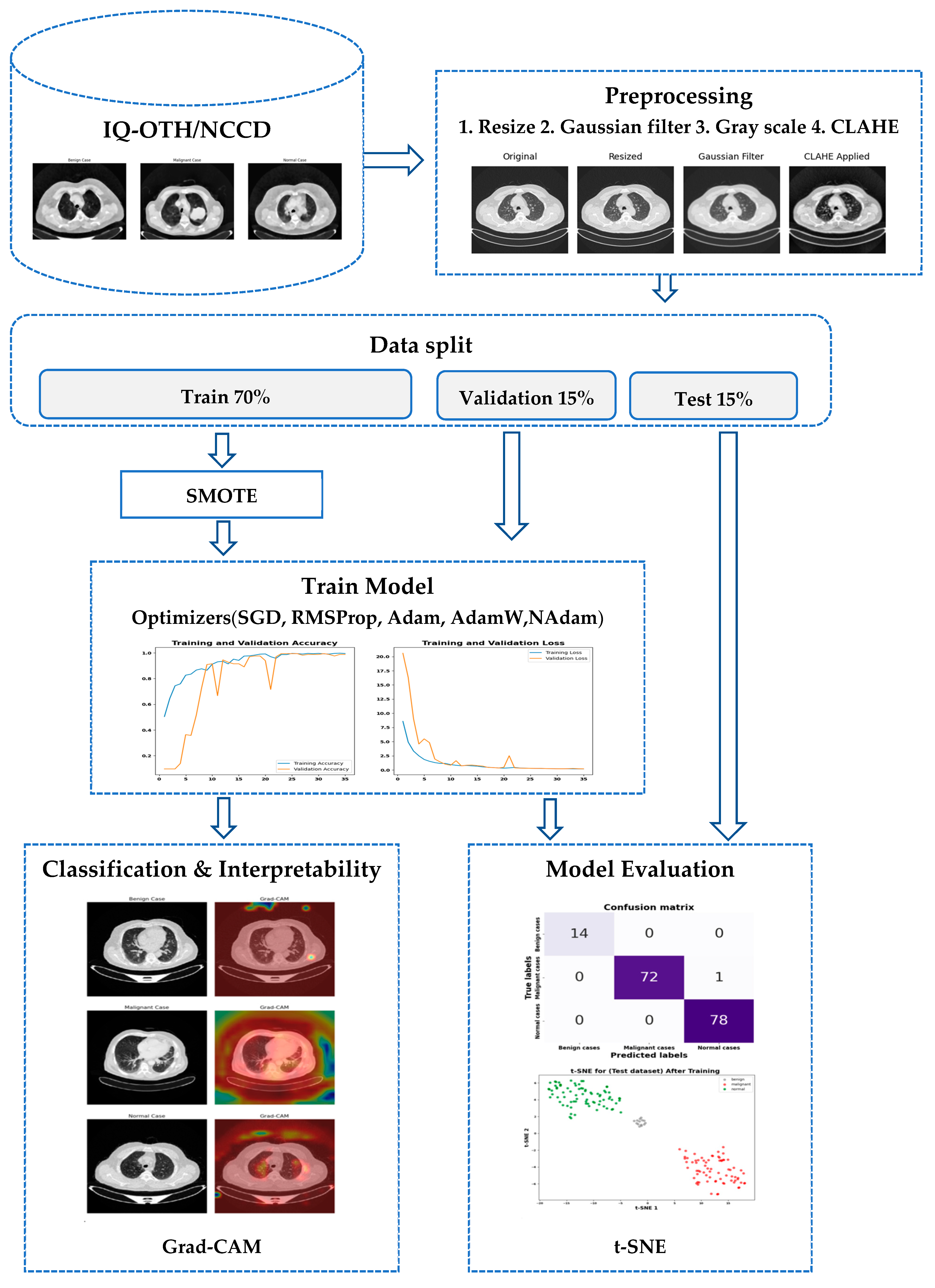
Figure 1. The block diagram of LCxNet Framework.
Asi 08 00153 g001
Figure 2. CT scan samples after a series of preprocessing steps—resizing, Gaussian filtering, and CLAHE—displaying (a) benign, (b) malignant, (c) normal.
Asi 08 00153 g002aAsi 08 00153 g002b
Figure 3. Histogram analysis for CLAHE-processed samples: (a) benign, (b) malignant, (c) normal.
Asi 08 00153 g003aAsi 08 00153 g003b
Figure 4. Training data distribution (a) before SMOTE and (b) after SMOTE.
Asi 08 00153 g004
Figure 5. Architecture of the LCxNet model for lung cancer detection.
Asi 08 00153 g005
Figure 6. AdamW weight decay impact on CT scan classification accuracy and loss.
Asi 08 00153 g006
Figure 7. Comparison of different optimizers based on test accuracy and loss values.
Asi 08 00153 g007
Figure 8. Training and validation for accuracy and loss diagram. (a) SGD, (b) RMSprop, (c) Adam, (d) AdamW, (e) NAdam.
Asi 08 00153 g008aAsi 08 00153 g008b
Figure 11. t-SNE visualization of the training data was performed with parameters (perplexity = 30, learning rate = auto, random state = 42, and number of iterations = 1000) for the Adam optimizer. (a) Before training, the raw LCxNet data appeared highly complex and entangled. (b) After training, the LCxNet effectively learned discriminative features, resulting in clear separation of clusters. (c) The test dataset visualization further demonstrates distinct separation among the three class clusters, indicating strong generalization of the model.
Asi 08 00153 g011
Figure 12. The Grad-CAM technique, with an alpha value of 0.5, produces visualizations in which the most important parts of the input image that significantly impact the model’s predictions are highlighted by regions in warmer colors. Cooler-colored areas, on the other hand, indicate less significant features. By using this visualization technique to differentiate between (a) benign, (b) malignant, and (c) normal conditions, the model’s decision-making process was revealed.
Asi 08 00153 g012
Figure 13. Optimizer comparison for accuracy vs. loss (aug_IQ Dataset).
Asi 08 00153 g013
Figure 14. Training and validation for accuracy and loss diagram (Adam).
Asi 08 00153 g014
Figure 15. Comparison of different optimizers based on test accuracy and loss values for LC25000 Dataset.
Asi 08 00153 g015
Table 1. Summary of related work in lung cancer detection.
Ref.DatasetMethodsClassAdvantagesLimitationsMetrics %
Shafi et al.
2022 [26]
LUNA 16
(888 images)
CNN + SVM2-Hybrid model enhances results-Small dataset
-Poor scalability
Acc = 94
Pre = 95
Recall = 94.5
F1-score = 94.5
Shaziya & Kattula
2023 [27]
LIDC-IDRI
(6691images)
CNN2-Specialized architecture for nodules-CT image size reduction impactAcc = 93.58
Sen = 95.61
Spe = 90.14
Mohamed et al. 2023 [28]IQ-OTH/NCCDEOSA-CNN3-Combines Ebola optimization for feature selection-Limited data
-Data imbalances
-Time complexity
Acc = 93.21
Pre =100
Sen = 90.7
Spe =100
F1-score = 92.7
Rajasekar et al. 2023 [29]-CT scan
-histopathological
(15,000 images)
CNN, CNN GD, Inception V3, Resnet-50, VGG-16, and VGG-19a-2
b-3
-CNN GD enables continuous parameter learning-Computational cost (400 epochs)For CNN GD Acc = 97.86
Pre = 96.39
Sen = 96.7
Spe = 97.4
F1-score = 97.9
Damayanti et al. 2023 [30]CT scanCNN + DenseNet3-Hybrid architecture improves feature extraction-Unknown no. of data Acc= 99.49
UrRehman et al. 2024 [31]LUNA16(CNN) With a dual attention mechanism2-Dual attention mechanism focuses on relevant node features-Increase training time
-Computational cost
Acc = 95.4
Pre = 95.8
Sen = 94.6
Spe = 93.1
Pathan et al.
2024 [32]
IQ-OTH/NCCDSCA-CNN3-Optimized architecture for high-precision classification
-Heatmap highlights anatomy
-Limited data
-High computational costs
Acc = 99
Pre = 92.4
Sen = 92
Spe = 99.1
F1-score = 93
Saxena et al. 2025 [33] CT scan
(434 images)
CNN2-Introduced Maximum Sensitivity Neural Network-Small dataset.
-Poor scalability
Acc = 98
Sen = 97
Alsallal et al. 2025 [34] CT scan
(2725 images)
Radiomic features with DL and attention mechanisms5-Hybrid improves accuracy-Complex model handlingAcc = 92.47
Sen = 92.11
AUC = 93.99
Table 2. Training data distribution before and after SMOTE.
Class TypeOriginal SamplesSMOTE Samples
Benign78385
Malignant385385
Normal304385
Total 7671155
Table 3. Convolutional neural network (CNN) architecture.
Layer (Type)Output ShapeParameters
Input(220, 220, 1)0
Conv2d(218, 218, 16)160
Batch normalization(218, 218, 16)64
Max_pooling2d(109,109,16)0
Conv2d_1(107, 107, 32)4640
Batch_normalization_1(107, 107, 32)128
Max_pooling2d_1(53, 53, 32)0
Conv2d_2(51, 51, 64)18,496
Batch_normalization_2(51, 51, 64)256
Max_pooling2d_2(25, 25, 64)0
Conv2d_3(23, 23, 128)73,856
Batch_normalization_3(23, 23, 128)512
Max_pooling2d_(11, 11, 128)0
Flatten(15488)0
Dense(256)3,965,184
Dropout(256)0
Dense_1(128)32,896
Dropout_1(128)0
Dense_2(3)387
Total Parameters 4,096,579 (15.63 MB)
Trainable Parameters 4,096,099 (15.63 MB)
Non-trainable Parameters 480 (1.88 KB)
Table 4. LCxNet model Hyperparameters.
Hyper-ParameterValue
Image size(220, 220, 1)
Batch size16
Learning rate0.001
OptimizerSGD, RMSProp, Adam, AdamW, NAdam
Epochs35
Loss functioncategorical_crossentropy
Early-stoppingmonitor = val_loss, patience = 7
ReduceLROnPlateaumonitor = val_loss, patience = 3, factor = 0.5
To improve model stability and generalization, regularization strategies such as dropout and L2 regularization—which are covered in the architecture section—also complement hyperparameter tuning.
Table 5. Comparison of LCxNet metrics across different optimizers.
OptimizerAccuracy %Weighted
Precision %
Weighted
F1-Score %
Weighted
Sensitivity %
Weighted
Specificity %
Cohen’s Kappa %LossMR %
SGD98.1898.2298.1398.1898.0896.743.961.82
RMSprop98.7998.8398.7798.7999.3997.970.071.21
Adam99.3999.4099.3999.3999.4698.940.170.61
AdamW99.3999.4299.4099.3999.8999.010.180.61
NAdam99.3999.4099.3999.3999.5598.960.190.61
Table 6. Comparison of the LCxNet model metrics across different data split ratios (Adam).
Split-RatioAccuracy %Weighted
Precision%
Weighted
F1-Score %
Weighted
Sensitivity %
Weighted
Specificity %
Cohen’s Kappa %LossMR %
70:15:1599.3999.4099.3999.3999.4698.940.180.61
80:10:1099.0999.1199.0999.0999.3098.530.140.91
80:2098.6498.7998.6798.6499.8397.710.221.36
Table 7. Comparison of model metrics across different optimizers (aug-IQ).
OptimizerAccuracy %Weighted
Precision %
Weighted
F1-Score %
Weighted
Sensitivity %
Weighted
Specificity %
Cohen’s Kappa %LossMR %
SGD95.7995.9495.7795.7997.7293.584.844.21
RMSprop95.5795.7895.5395.5797.6293.250.204.43
Adam96.7796.8695.9996.7798.2595.080.203.23
AdamW96.8897.0496.8696.8898.3295.240.183.12
NAdam95.7995.9795.7595.7997.7393.580.224.21
Table 8. Comparison of model metrics across different optimizers (LC25000 dataset).
OptimizerAccuracy %Weighted
Precision %
Weighted
F1-Score %
Weighted
Sensitivity %
Weighted
Specificity %
Cohen’s Kappa %LossMR %
SGD96.7696.8096.7596.7698.4095.130.273.24
RMSprop97.8297.8297.8297.8298.9296.730.072.18
Adam98.2798.2798.2698.2799.1497.400.071.73
AdamW98.3198.3198.3198.3199.1497.470.081.69
NAdam97.7897.8297.7897.7898.9096.670.112.22
Table 9. Performance comparison of the model using different techniques and parameters.
ModelAccuracy %Weighted
Precision %
Weighted
F1-Score %
Weighted
Sensitivity %
Weighted
Specificity %
Cohen’s Kappa %LossMR
%
Total
Parameters
VGG1695.7695.6795.6595.7697.5092.340.194.2414,718,275
ResNet5093.9493.9393.9393.9496.5289.160.246.0623,602,051
MobileNetV296.9797.4497.1296.9798.7894.650.083.032,266,947
InceptionV392.7393.7093.1092.7396.7687.220.217.2721,817,123
DenseNet12196.3696.3196.2896.3697.9993.450.113.647,044,675
Xception95.7696.4795.9395.7698.1592.510.1495.7620,875,819
Proposed LCxNet 99.3999.4099.3999.3999.4698.940.180.614,096,579
Disclaimer/Publisher’s Note: The statements, opinions and data contained in all publications are solely those of the individual author(s) and contributor(s) and not of MDPI and/or the editor(s). MDPI and/or the editor(s) disclaim responsibility for any injury to people or property resulting from any ideas, methods, instructions or products referred to in the content.