Article

Fault Diagnosis in Internal Combustion Engines Using Artificial Intelligence Predictive Models

by
Norah Nadia Sánchez Torres
1,
Joylan Nunes Maciel
1,
Thyago Leite de Vasconcelos Lima
2,
Mario Gazziro
3,
Abel Cavalcante Lima Filho
4,
João Paulo Pereira do Carmo
5 and
Oswaldo Hideo Ando Junior
1,2,4,6,*
1
Interdisciplinary Postgraduate Program in Energy & Sustainability (PPGIES), Federal University of Latin American Integration—UNILA, Foz do Iguaçu 85867-000, PR, Brazil
2
Federal Institute of Education, Science and Technology of Paraiba (IFPB), Campus João Pessoa, João Pessoa 58015-435, PB, Brazil
3
Information Engineering Group, Department of Engineering and Social Sciences (CECS), Federal University of ABC (UFABC), Santo André 09210-580, SP, Brazil
4
Postgraduate Program of Mechanical Engineering (DEME), Technology Center (CT), Federal University of Paraiba (UFPB), Jardim Universitário, s/n, João Pessoa 58051-900, PB, Brazil
5
Group of Metamaterials Microwaves and Optics (GMeta), Department of Electrical Engineering (SEL), University of São Paulo (USP), São Carlos 13566-590, SP, Brazil
6
Center for Alternative and Renewable Research (CEAR), Federal University of Paraiba (UFPB), João Pessoa 58051-900, PB, Brazil
*
Author to whom correspondence should be addressed.
Appl. Syst. Innov. 2025, 8(5), 147; https://doi.org/10.3390/asi8050147
Submission received: 22 August 2025 / Revised: 13 September 2025 / Accepted: 25 September 2025 / Published: 30 September 2025

Abstract

The growth of greenhouse gas emissions, driven by the use of internal combustion engines (ICE), highlights the urgent need for sustainable solutions, particularly in the shipping sector. Non-invasive predictive maintenance using acoustic signal analysis has emerged as a promising strategy for fault diagnosis in ICEs. In this context, the present study proposes a hybrid Deep Learning (DL) model and provides a novel publicly available dataset containing real operational sound samples of ICEs, labeled across 12 distinct fault subclasses. The methodology encompassed dataset construction, signal preprocessing using log-mel spectrograms, and the evaluation of several Machine Learning (ML) and DL models. Among the evaluated architectures, the proposed hybrid model, BiGRUT (Bidirectional GRU + Transformer), achieved the best performance, with an accuracy of 97.3%. This architecture leverages the multi-attention capability of Transformers and the sequential memory strength of GRUs, enhancing robustness in complex fault scenarios such as combined and mechanical anomalies. The results demonstrate the superiority of DL models over traditional ML approaches in acoustic-based ICE fault detection. Furthermore, the dataset and hybrid model introduced in this study contribute toward the development of scalable real-time diagnostic systems for sustainable and intelligent maintenance in transportation systems.

1. Introduction

The climate crisis has brought to the forefront greenhouse gas emissions in the renewed conversation regarding energy sustainability. In 2023, worldwide GHG emissions reached 57.1 gigatons of carbon dioxide equivalent, a 1.3% increase over the figure for 2022. The energy industry with 15.1 GtCO2e and the transport sector with an emissions volume of 8.4 GtCO2e [1] were high level sources too. Maritime transport has particularly alarming features with regard to emissions. Just 25,000 vessels—only representing 30% of the world’s fleet—accounted for as much as 80% of carbon dioxide emissions from the industry, according to a study conducted by Det Norske Veritas in 2019. Even more alarming is that 93% of today’s global fleet still runs exclusively on fossil fuels [2].
The International Maritime Organization released projections in 2020 showing that, if we do not act, these emissions could reach 90% to 130% of the 2008 levels by 2050 [3]. With this future, the IMO has ambitious goals: to significantly reduce carbon emissions by 2050; to reduce emissions by 20% by 2030, and to reduce emissions by 70% by 2040 [3].
Nowadays, Brazil has a fleet of vehicles equipped with internal combustion engines, and so does the rest of the world. From a technical standpoint, this dependence on the sector teaches us exactly how urgent it is to originate green alternatives in this sector. Brazil has committed to global targets under the 2030 Agenda for Sustainable Development, and in relation to the Paris Agreement, with a goal of carbon neutrality by 2050 and reducing CO2 emissions by 37% (2025) and 43% (2030) [4,5,6].
Internal combustion engines (ICEs) emerge as strategic tools to foster reduction emissions and to improve the efficiency of ICEs. The use of AI-based methods helps in the early recognition of operational irregularities, which helps to reduce energy loss and avoid mechanical disfunction.
In this context, Artificial Intelligence (AI) offers the ability to process large volumes of complex sensor data efficiently and in real time. Data-driven approaches such as Machine Learning and Deep Learning have significantly advanced the ability to model and understand such complexities, overcoming the limitations of analyses that are restricted to generic information, such as basic ship characteristics. In particular, Deep Learning (DL) models excel in handling audio signals by automatically extracting relevant features from raw data, detecting temporal patterns, and enabling real-time scalable diagnostic systems.
The most frequently investigated faults include mechanical problems, lubrication system faults, and cooling system faults. Mechanical faults may include valve clearance difficulties, ignition faults, and fuel injection difficulties. Lubrication system failures are often associated with variations in oil pressure and viscosity, while cooling system failures include water leaks and engine overheating [6,7,8]. Some authors point out that vibration and acoustic measurements are among the most effective non-invasive or non-destructive techniques used to diagnose failures [9,10,11,12,13]. Regardless of the approach chosen, both measures correspond to time series, which represent sequences of observations collected at regular time intervals, allowing the analysis of temporal dependency patterns, such as trend, zonality, and autocorrelation [14].
For vibration analysis, Fast Fourier Transform (FFT) has proven crucial for the diagnosis of rotating machines. FFT is an efficient algorithm for computing the Discrete Fourier Transform (DFT), enabling the decomposition of time-domain signals into their spectral components while reducing the computational complexity from O(N2) to O(N log N) [15]. FFT is particularly effective in detecting resonance frequencies and identifying harmonic components associated with imbalances, misalignments, and other mechanical faults common in ICEs.
Recent studies show that spectral analysis techniques using FFT can identify characteristic failure patterns in internal combustion engines by analyzing vibration signals [16]. The study highlights that high vibration levels in centrifugal loop dryer machines hinder real-time operational monitoring. The application of the FFT [15] addresses this issue by decomposing vibration signals into their constituent frequencies, enabling the identification of fault patterns and inadequate damping. Consequently, FFT reduces measurement uncertainty and supports structural and operational adjustments, thereby reinforcing the study’s statistical and theoretical analysis [16].
On the other hand, a critical aspect that is often overlooked in the analysis of acoustic and vibration signals is the consideration of noise and measurement errors. Accurate determination of the instantaneous noise level and quantification of potential measurement errors are fundamental to the development of reliable diagnostic systems. Recent studies show that variations in noise levels can have a significant influence on the accuracy of diagnostic models, particularly in dynamic operating environments [17]. Variables such as the acceleration, speed, and operating density can induce sudden fluctuations in noise levels, affecting the quality of the data collected for subsequent analysis.
In the acoustic domain, such spectral components, although attenuated by propagation and masking, preserve correlations with operating conditions and failure mechanisms, thereby justifying time–frequency representations (e.g., log-Mel) that capture both harmonic content and transient events [18].
Under real operating conditions, variations in ambient noise and the dynamics of adjacent traffic/flows directly affect the data quality and the reliability of inferences. Approaches for determining the instantaneous noise level and estimating measurement errors demonstrate how acceleration, velocity, and operational density can induce abrupt fluctuations in sound levels, compromising accuracy metrics if noise is not properly controlled and modeled [15]. Consequently, strategies for data acquisition, calibration, and noise enrichment become intrinsic components of robust pipelines for audio-based predictive maintenance.
Given these challenges and considering the advances in the use of Artificial Intelligence (AI), there is a lack of studies that advance the development of solutions aimed at the predictive maintenance of embedded systems, especially with ICE. There is also a scarcity of public datasets containing structured and labeled faults that allow the development of solutions using robust Deep Learning (DL) models [19]. Therefore, this study aims to present and make available a new labeled dataset with ICE fault sound signals and, mainly, to evaluate the performance of different ML and DL models in detecting these faults through sound analysis. In addition, a new hybrid model based on GRU and Transformers [20] is proposed to improve the detection capability, accuracy, and computational efficiency in non-invasive ICE monitoring.
Traditional AI models, such as Artificial Neural Networks (ANNs), have proven effective in capturing and recognizing complex patterns even with noisy data, providing personalized diagnoses [21,22]. More recently, DL algorithms such as Support Vector Machines (SVMs), Probabilistic Neural Networks (PNNs), Multi-Layer Perceptron (MLP), Convolutional Neural Networks (CNNs), and Recurrent Networks, such as Long-Short Term Network (LSTM) and Gated Recurrent Units (GRUs), have been successfully employed in different classification and fault prediction tasks [23,24,25,26,27,28,29,30,31]. Signal processing techniques such as FFT and Discrete Wavelet Transform (DWT) are commonly used to filter noise and identify patterns in acoustic signals, with FFT being particularly relevant for analyzing vibration frequencies in rotating machinery [16,32]. Recent studies also highlight the use of CNNs with transfer learning [14], multivariate LSTMs [26], and Variational Autoencoders (VAEs) [33,34,35], as effective methods for detecting anomalies and operational failures in vessels. However, there is a significant gap in terms of the scarcity and quality of public datasets, including the number of failure types. In addition, most studies use private data, limiting the reproducibility and comparison of results.
Therefore, this study aims to develop and evaluate an efficient non-invasive fault detection system for internal combustion engines (ICEs) based on acoustic signal analysis. The research proposes and tests a new hybrid deep learning model—BiGRUT—capable of accurately identifying multiple types of ICE failures, even under complex and overlapping conditions. Additionally, it introduces a new labeled and publicly available dataset to support reproducible experimentation and benchmarking.
The main contributions of this work are summarized below: (i) Novel Dataset for ICE Faults: a structured and labeled dataset of 2184 audio samples covering 12 fault subclasses, recorded under controlled conditions and made publicly available for future research. (ii) Comprehensive Model Evaluation: a comparative analysis of 10 ML and DL models—including CNN, GRU, LSTM, and Transformer—using rigorous metrics such as accuracy, precision, recall, F1-score, and MCC. (iii) Proposal of BiGRUT Architecture: introduction of a hybrid model combining GRU and Transformer mechanisms, which outperforms all evaluated baselines across most metrics. (iv) Robustness Across Fault Types: detailed performance analysis by failure type (mechanical, misfires, and combined faults), highlighting the model’s stability and generalization capability. (v) Sustainability-Oriented Vision: discussion on how acoustic diagnostics can support predictive maintenance and contribute to broader goals of CO2 reduction and operational efficiency.
Finally, this study is structured into five sections covering the different aspects explored. Section 2 discusses the theoretical basis for vessel failures, the fundamentals of audio-based predictive maintenance, and a review of DL architectures. Section 3 presents the materials and methods used, detailing the database used and provided, the experimental procedures, the evaluation metrics applied, and the proposal for a new hybrid model (BiGRUT) for fault classification. Section 4 presents the results obtained, comparing the performance between the different architectures, with emphasis on the hybrid proposal. Finally, Section 5 brings together the conclusions of the study, academic and practical contributions, limitations, and future research.

2. Theoretical Background

This section presents the theoretical foundations necessary to understand the context and challenges of fault diagnosis in internal combustion engines (ICE) using artificial intelligence techniques. It first discusses the main categories of ICE faults and the principles of predictive maintenance, with emphasis on non-invasive diagnostic approaches such as vibration and acoustic analysis. Then, a review of traditional machine learning (ML) models and recent advances in deep learning (DL) architectures is provided, focusing on their application to fault classification tasks. This theoretical overview supports the methodological choices and model development proposed in this paper and lays the groundwork for the comparative evaluation presented in the following sections.

2.1. Faults in Internal Combustion Engines

Internal combustion engines (ICE) are subject to failures that compromise their operation, efficiency, and durability. In applications for the shipping sector, the most common anomalies are of mechanical nature [6,7,8], lubrication [36,37], ignition [38,39], fuel injection [40], cooling [8], and combustion/emissions [41,42].
Predictive maintenance, based on the early detection of faults using operational data, aims to anticipate failures and prevent breakdowns. Its benefits include cost reduction and avoidance of unplanned downtime [43,44,45,46], as well as increased safety and asset lifetime [44,47]. However, its implementation faces significant challenges: the need for robust sensors, the complexity of signal analysis under variable conditions, the generalization of diagnostic models, and the scarcity of public datasets for the development of AI algorithms [21,22,23,24,25,32,48].
Diagnostic methods are divided into invasive and non-invasive approaches. Invasive methods (e.g., in-cylinder pressure measurement), although accurate, involve high costs, risks, and downtime [36,37]. In contrast, non-invasive methods monitor the engine externally through sensors (vibration, sound, temperature), allowing continuous, safe, and lower-cost diagnosis [6,7,9,10,11,12,13].
In data-driven automotive diagnostic systems, signal acquisition is a fundamental step, with non-invasive approaches standing out, including the following: (i) acoustic analysis via microphone, capable of identifying ignition or knocking faults with up to 99% accuracy [49,50,51]; vibration measurement using accelerometers, effective in detecting valve clearance issues and misalignments [32,39,52,53,54]; (ii) thermometry (mainly in exhaust gases), where variations indicate combustion faults, including advanced techniques such as ultrasonic thermometry [41,55,56]; (iii) current monitoring in actuators (e.g., fuel injectors) for electromechanical failures [40]; and (iv) thermal imaging and ultrasound for oil thickness assessment and hotspot detection [42,57].
In summary, the integration of vibration (FFT) and acoustics, combined with sensor calibration practices, uncertainty quantification and noise modeling, constitutes the methodological basis for replicable non-invasive diagnostics. This integration informs choices of Short-Time Fourier Transform (STFT) windows, honeybands, and sampling regimes, which, in turn, preserve relevant harmonic and transient signatures in ECIs [16,17].

2.2. Machine Learning Predictive Models

Machine Learning (ML) models have been consolidated as powerful tools for analyzing, classifying, and predicting patterns in complex and high-dimensional data. Their application in diagnostic systems, particularly in the context of mechanical and acoustic engineering, enables automatic anomaly and fault detection with high accuracy, even in noisy scenarios or under significant temporal variability [58].
Among the most widely used algorithms are traditional methods rooted in statistics and decision theory, as well as more recent techniques incorporating nonlinear neural architectures. Each model presents specific characteristics in terms of its generalization capacity, noise sensitivity, interpretability, and computational cost. This justifies comparative analyses of different approaches for specific tasks, such as acoustic fault classification in ICEs [59]. The following subsections present some of the main ML models applied to engine fault classification from audio signals.

2.2.1. Decision Tree

Decision Trees (DT) are hierarchical models that iteratively partition the feature space based on impurity measures such as the Gini index or Entropy [60]. The resulting structure is interpretable and allows for easy mapping of the decisions made to classify an instance, making DTs particularly useful in environments where explainability is critical [19].
Despite their simplicity and computational efficiency, single decision trees tend to overfit, especially in datasets with high noise or variability. However, when properly parameterized (with limited depth, pruning, and balanced splitting), they can be effective in identifying clear patterns in audio signals associated with different subclasses of mechanical faults [19].

2.2.2. Gradient Boosting

Gradient Boosting (GB) is another ensemble method that sequentially builds weak learners, typically shallow decision trees, by optimizing a loss function through gradient descent. Unlike Random Forest, which explores parallelism, GB emphasizes iterative correction of errors from previous models to build a more accurate predictor [19].
This method demonstrates excellent performance in supervised tasks with heterogeneous data and is sensitive to hyperparameter tuning, particularly the learning rate, tree depth, and number of iterations. In the context of audio fault classification, its ability to capture residual patterns and handle noise can be leveraged to increase accuracy in distinguishing subtle signal variations [19].

2.2.3. Random Forest

Random Forest (RF) is an ensemble learning technique based on decision trees that improves the predictive accuracy by combining multiple trees trained independently on random subsets of data and features. This approach reduces the variance and enhances the generalization, particularly in multi-class tasks and noisy data, as commonly observed in acoustic fault diagnostics [19].
Each tree in the forest is trained using bootstrap samples and a random subset of features, promoting diversity within the ensemble. The final prediction is obtained by majority voting among trees. In addition to robustness, RF provides variable importance measures, which are valuable for interpretability and feature selection in acoustic signal analysis [19].

2.2.4. K-Nearest Neighbors

The k-Nearest Neighbors (k-NN) algorithm is an instance-based method that classifies a new sample according to the categories of its k closest neighbors in the feature space [56]. Its simplicity lies in the absence of an explicit training phase: the model stores the data and performs classification decisions during inference [19].
Although computationally expensive for large datasets, k-NN is effective when data exhibit natural clustering and when the feature space is well normalized. In acoustic fault recognition, k-NN can be particularly useful when fault patterns present spectral and temporal similarities, provided that a well-defined distance metric (e.g., Euclidean or Minkowski) is employed [19].

2.2.5. ANN-MLP

Using Artificial Intelligence (AI) [19], Artificial Neural Networks (ANNs) form the foundation for most Deep Learning (DL) models, being inspired by the functioning of the human brain. An ANN is composed of layers of interconnected neurons, suitable for learning complex patterns through the adjustment of synaptic weights during training [61]. The Multi-Layer Perceptron (MLP) is a type of ANN composed of densely connected layers and trained with the backpropagation algorithm, which adjusts synaptic weights to minimize the error between the predicted and true outputs [19].
The ability of MLPs to model complex nonlinear relationships makes them applicable to high-dimensional data and non-stationary signals, such as those found in audio-based diagnostics. The performance of MLPs depends on the architecture (number of layers and neurons), activation function, regularization, and learning rate, requiring careful tuning to avoid overfitting and ensure good generalization [19].

2.3. Deep Learning Predictive Models

Deep Learning (DL) predictive models consist of more than one hidden layer, organized in deeply nested network architectures. Moreover, they typically contain advanced neurons, in contrast to simple ANNs. In other words, DL models may employ advanced operations (e.g., convolutions) or multiple activations within a neuron, rather than a single activation function. These features enable DL models to be fed with raw input data and automatically discover the necessary representation for the corresponding learning task [53].
Machine learning is particularly useful in domains with large-scale high-dimensional data, which explains why DL outperforms shallow ML algorithms in most applications where text, image, video, speech, and audio data must be processed [61]. The following subsections present some of the main DL models employed in the classification of ICE faults from audio signals.

2.3.1. Recurrent Neural Networks

Recurrent Neural Networks (RNNs) are architectures designed to model sequential data, using recurrent connections between neurons that feed the output of a given time step as input to the next [62]. They are well-suited for capturing temporal dependencies in tasks such as speech recognition, time-series prediction, and natural language processing. However, they suffer from the vanishing gradient problem in long sequences, where training gradients become negligible when propagated backward through layers, preventing efficient weight updates and hindering the retention of long-term information [63,64].
Long Short-Term Memory (LSTM) networks were introduced to overcome the vanishing gradient problem in RNNs [65], allowing for the effective modeling of long-term dependencies [66]. They operate through three gates (input, forget, and output) that selectively control information flow, maintaining and updating an extended internal state [66,67,68,69]. LSTMs are widely used for modeling complex sequences (e.g., machine translation, temporal analysis), though they require higher computational cost due to the complexity of gating mechanisms [67].
Gated Recurrent Units (GRUs) were proposed as a simplified alternative to LSTMs, while still effectively capturing temporal dependencies [70]. GRUs employ only two gates (update and reset) and a single hidden state to retain relevant information and discard redundancies [66,67,68,69,71]. They achieve performance comparable to LSTMs in tasks such as natural language processing, while reducing the computational complexity by eliminating the separate cell state, resulting in faster training without significant loss of effectiveness [72].
The choice between LSTM and GRU depends on the balance required between the architectural complexity and task-specific demands [66]. A graphical representation of RNN, LSTM, and GRU architectures is provided in Figure 1.

2.3.2. Convolutional Neural Networks

Convolutional Neural Networks (CNNs) are specialized architectures designed to process data with spatial structure, such as images or time–frequency representations of signals (e.g., audio MFCCs) [61]. They are mainly applied to classification tasks in computer vision (autonomous vehicles, drones, medical diagnostics) and are extensively used for industrial signal analysis (vibration, sound), leveraging their ability to automatically extract hierarchical discriminative features through convolutional and pooling operations [61,73].
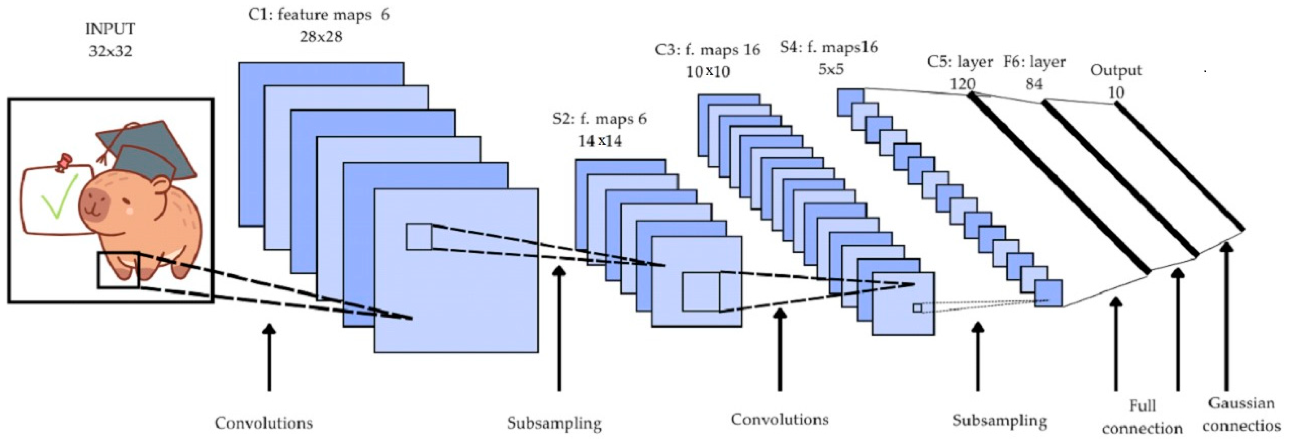
Their operation is based on sequential layers: convolutional layers apply filters to detect local patterns; pooling layers reduce dimensionality, ensuring invariance to small variations; and fully connected layers perform the final classification. As exemplified in Figure 2, a typical CNN (e.g., LeNet for digit recognition) begins with progressive feature extraction (C1, S2, C3, S4), followed by higher-level abstraction layers (C5, F6), and a classification output [74].
CNNs address the problem of complex pattern recognition in multidimensional data, offering superior generalization and parameter efficiency compared to dense networks, due to weight sharing and the hierarchical nature of learned features [74]. However, their effectiveness can be compromised by overfitting in small or imbalanced datasets, requiring techniques such as data augmentation and regularization [75,76].

2.3.3. Transformers

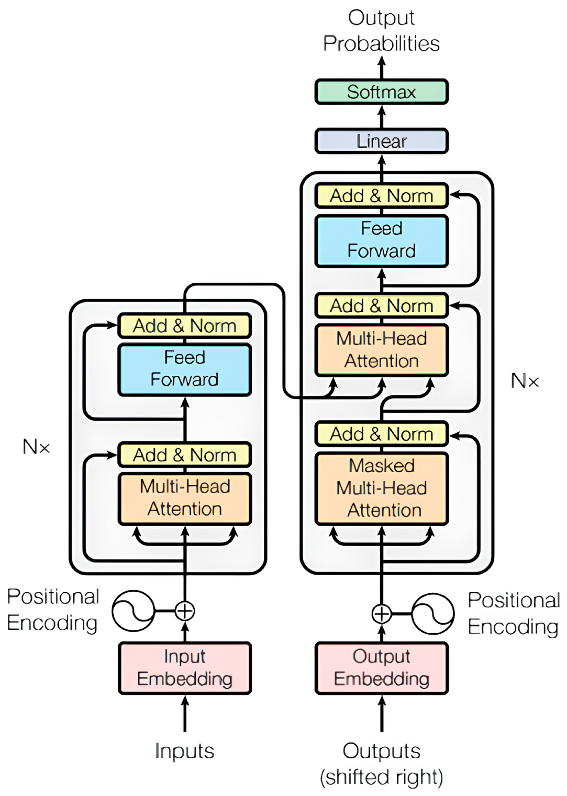
Another approach introduced by Vaswani et al. [20] in 2017 is the Transformer architecture, which is based on self-attention mechanisms designed to capture long-range dependencies in sequential data. Transformers serve as an efficient alternative to RNNs by overcoming the limitations of sequential processing, as they allow parallel computation across the entire sequence. This significantly improves the computational efficiency and reduces the training time [77].
The encoder processes the input through multi-head self-attention layers (calculated using Equation (1)), followed by fully connected feed-forward networks, employing residual connections [78] and normalization techniques to stabilize training [79].
A t t e n t i o n Q , K , V = s o f t m a x   Q × K T d k X V ,
where Q, K, and V are the query, key, and value matrices, respectively, and dk is the dimensionality of the keys. Subsequently, the decoder generates the sequential output, incorporating a third sublayer that applies attention over the encoder’s output [20,80,81,82,83]. This architecture eliminates the need for the iterative processing typical of RNNs, enabling simultaneous and robust contextual learning in tasks such as machine translation and language analysis, with remarkable performance gains in long sequences [20,68]. The Transformer architecture is illustrated in Figure 3.

2.4. Classification Measures

In the evaluation of DL models applied to classification tasks, standardized metrics are employed to quantify different aspects of predictive performance. The confusion matrix is an essential tool for interpretative analysis, allowing the identification of systematic errors, prioritization of critical classes, and validation of data-balancing strategies [84,85,86,87].
In a confusion matrix (Appendix A, Table A1), the predictions of a binary classification model are compared across four categories: True Positive (TP): cases where the model correctly predicted the positive class, and the true class is also positive. False Positive (FP): cases where the model incorrectly predicted the positive class, while the true class is negative. True Negative (TN): cases where the model correctly predicted the negative class, and the true class is also negative. and False Negative (FN): cases where the model incorrectly predicted the negative class, while the true class is actually positive.
From the confusion matrix, it is possible to derive metrics such as accuracy, precision, recall, F1-score, and Matthews Correlation Coefficient (MCC). Accuracy represents the proportion of correct predictions relative to the total number of samples, as shown in Equation (2). However, this metric can be influenced by imbalanced datasets, favoring majority classes. Precision (Equation (3)) evaluates the model’s ability to minimize false positives, indicating the proportion of correctly classified positive samples relative to all positive predictions. Recall (Sensitivity) (Equation (4)) measures the model’s efficiency in identifying all true positive instances, being less sensitive to imbalanced distributions. F1-score (Equation (5)) combines precision and recall as a harmonic mean, providing a single measure of performance. Matthews Correlation Coefficient (MCC) (Equation (6)) is a robust evaluation metric for binary classifiers, as it considers all elements of the confusion matrix (TP, TN, FP, FN) [88,89,90]. Unlike accuracy or F1-score, MCC is immune to class imbalance and ranges from –1 (total disagreement/inverse classification) to +1 (perfect classification), with 0 indicating random prediction.
A c u r a c c y = T P + T N T P + T N + F P + F N
P r e c i s i o n = T P i T P i + F P i
R e c a l l = T P T P + F N
F 1 s c o r e = 2 R e c a l l P r e c i s i o n R e c a l l + P r e c i s i o n
M C C = T N T P F N F P T P + F P T P + F N T N + F P ( T N + F N )
Taken together, these metrics provide a robust and multidimensional assessment of classification model effectiveness.

2.5. Key Studies in the Scientific Literature

Non-invasive methods combined with AI have proven increasingly effective in detecting faults in ICEs. The review study presented in [48] highlights that 47% of the works analyzed address mechanical faults, 21% ignition faults, 16% combined ignition and injection faults, 16% injection-only faults, and 5% oil film thickness. The most commonly used acquisition systems include sound, vibration, temperature, current, and oil sensors. Moreover, ref. [48] emphasizes the growing use of neural network architectures for diagnostic and predictive maintenance, the relevance of the sampling rate, and the scarcity of public datasets, which limits the reproducibility of studies.
Sound and vibration signals are widely employed to identify mechanical faults in ICEs, as demonstrated in [24,32,54,91]. In [54], piezoelectric sensors and FFT/DFT were applied for ignition fault analysis. Meanwhile, ref. [24] employed DWT with PNN to separate noise and improve classification accuracy, highlighting the efficiency of the Meyer wavelet. Study [91] proposed a system for ICEs in the shipping sector using SVM, achieving 100% reliability, while [32] applied FFT with SVM in MATLAB, obtaining 97% accuracy.
Acoustic signals are also emphasized in [12,50,51,92], with different processing techniques. In [12], decision trees analyzed acoustic spectra, while [92] employed sound sensors to detect injection misfires in ICEs in the shipping sector. The work in [50] integrated low-cost hardware and smartphone-based ANN analysis, achieving 99.58% accuracy. Similarly, ref. [51], proposed a multitask CNN for detecting ignition faults using sound captured via smartphone, achieving 87% accuracy.
The fusion of multisensory signals is addressed in [57], where CNNs were used to integrate vibration and pressure data, improving diagnostics under variable operational conditions. Hybrid models have also gained attention. The author of [33], proposed an unsupervised model based on VAEs, testing several encoder–decoder architectures with real unlabeled data and achieving over 99% accuracy. In [34,35], the model was expanded to online fault diagnosis, independent of fault type, using multi-regime normalization and achieving an accuracy above 97%.
In ref. [93], a supervised 1D-CNN was applied to monitor ICEs in the shipping sector with data collected over 32 months, classifying seven operational states with up to 100% accuracy. The authors of [26] employed both supervised and unsupervised models (LSTM, One-Class SVM, XGBoost, WPE) on real data to predict bearing corrosion faults, demonstrating that ensembles increase alert robustness. For ship propulsion systems (SPS), ref. [28] tested DNN, LSTM, and GRU with simulated data, achieving an accuracy above 99% even under noise and load variations. Finally, ref. [27] proposed an online diagnostic approach using Transfer CNN, integrating offline networks with an optimized online CNN (LeNet-5) applied to public datasets. Inputs were vibration signals converted into images, achieving accuracy above 99% in detecting various faults in bearings and pumps.
This systematic review demonstrated the potential of non-invasive AI-based methods, particularly those combining vibration and acoustic analysis with DL architectures such as CNNs and VAEs, for fault detection in ICEs. Most studies reported accuracies above 95%. However, a critical analysis of the literature revealed four major challenges that limit the advancement and applicability of these techniques: (i) reproducibility issues, since 75% of the studies analyzed (12/16) employ non-public datasets; (ii) lack of methodological standardization, with no unified protocols for comparative evaluation; (iii) scarcity of studies addressing diverse fault types under varying operational conditions; and (iv) lack of joint evaluation of ML and DL models for comprehensive ICE fault classification.
Therefore, the present study represents an important step toward transforming theoretical advances into robust and reproducible solutions for real-world predictive maintenance problems, making the following contributions: (i) provision of a new structured, standardized, and labeled dataset; (ii) accuracy analysis of fault identification using various ML and DL models; and (iii) proposal and evaluation of a hybrid model (BiGRUT) for fault classification.
Taken together, the models and techniques reviewed in this section establish the theoretical foundation for the predictive maintenance approach proposed in this study. By integrating established machine learning methods and advanced deep learning architectures, such as CNNs, GRUs, and Transformers, this work aims to address complex ICE fault patterns through non-invasive acoustic signal analysis. Moreover, these models will be comparatively evaluated in Section 4, based on a newly constructed and publicly available dataset. This contextual and methodological alignment ensures a robust framework for benchmarking intelligent diagnostic systems in real-world ICE applications.

3. Materials and Methods

This section details the methodological framework adopted in this study, encompassing dataset construction, experimental setup, signal preprocessing, model development, and evaluation metrics. The goal is to ensure a transparent and reproducible process for assessing the performance of ML and DL models in the detection of internal combustion engine (ICE) faults using acoustic signals. Additionally, the architecture and motivation for the proposed BiGRUT hybrid model, combining Gated Recurrent Units (GRU) and Transformer layers, are presented and justified in the context of non-invasive fault diagnosis.

3.1. Dataset and ICE Failures

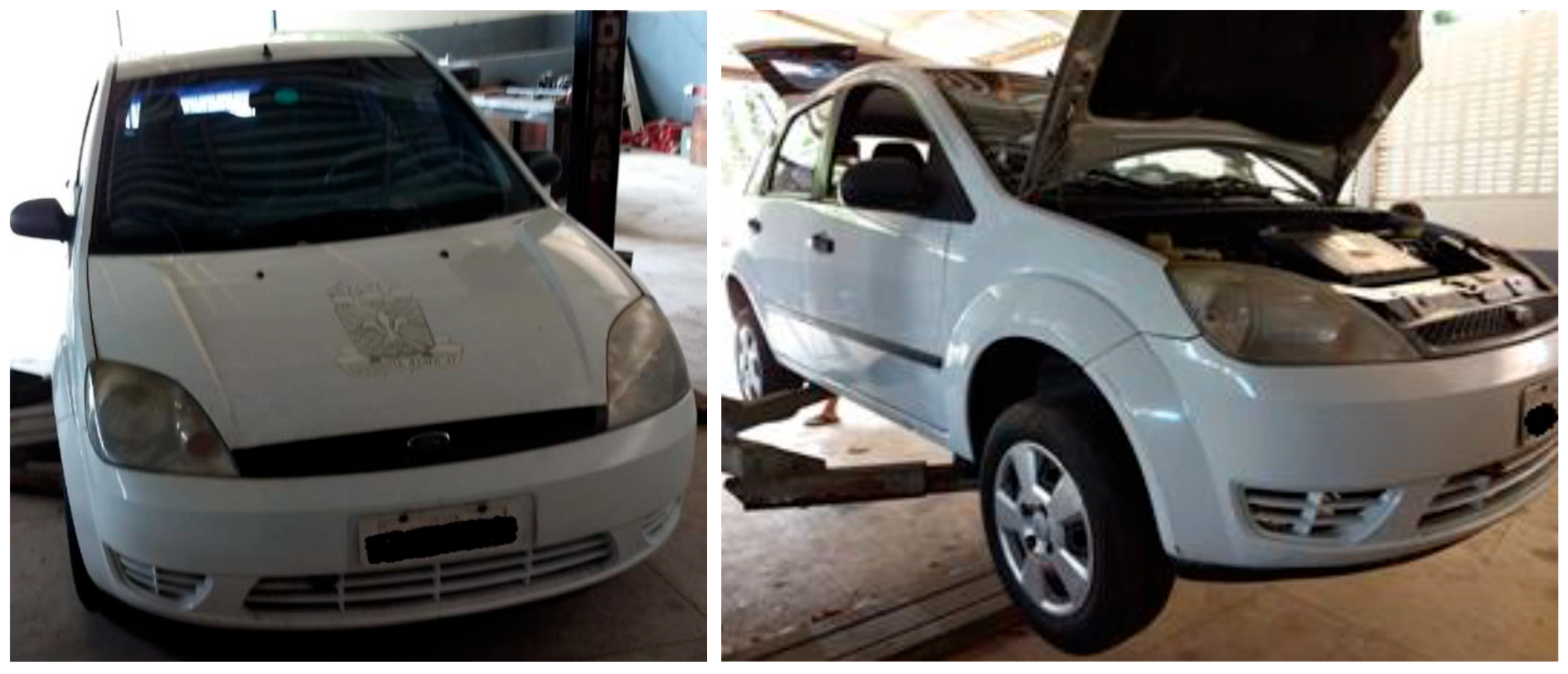
The data used in this study were experimentally collected from tests on an internal combustion engine (Otto cycle, four-stroke, spark ignition) carried out at the Engine Laboratory of the Department of Mechanical Engineering, under controlled conditions to ensure test reproducibility [94]. The engine was installed in a 2005 Ford Fiesta 1.6 vehicle, as shown in Figure 4, which is part of the laboratory fleet at the Federal University of Paraíba (UFPB).
The acquisition of acoustic signals was performed near the vehicle’s exhaust system, with an electret microphone positioned approximately one meter away at a 45° angle relative to the gas outlet, in order to capture sound characteristics representative of engine operation.
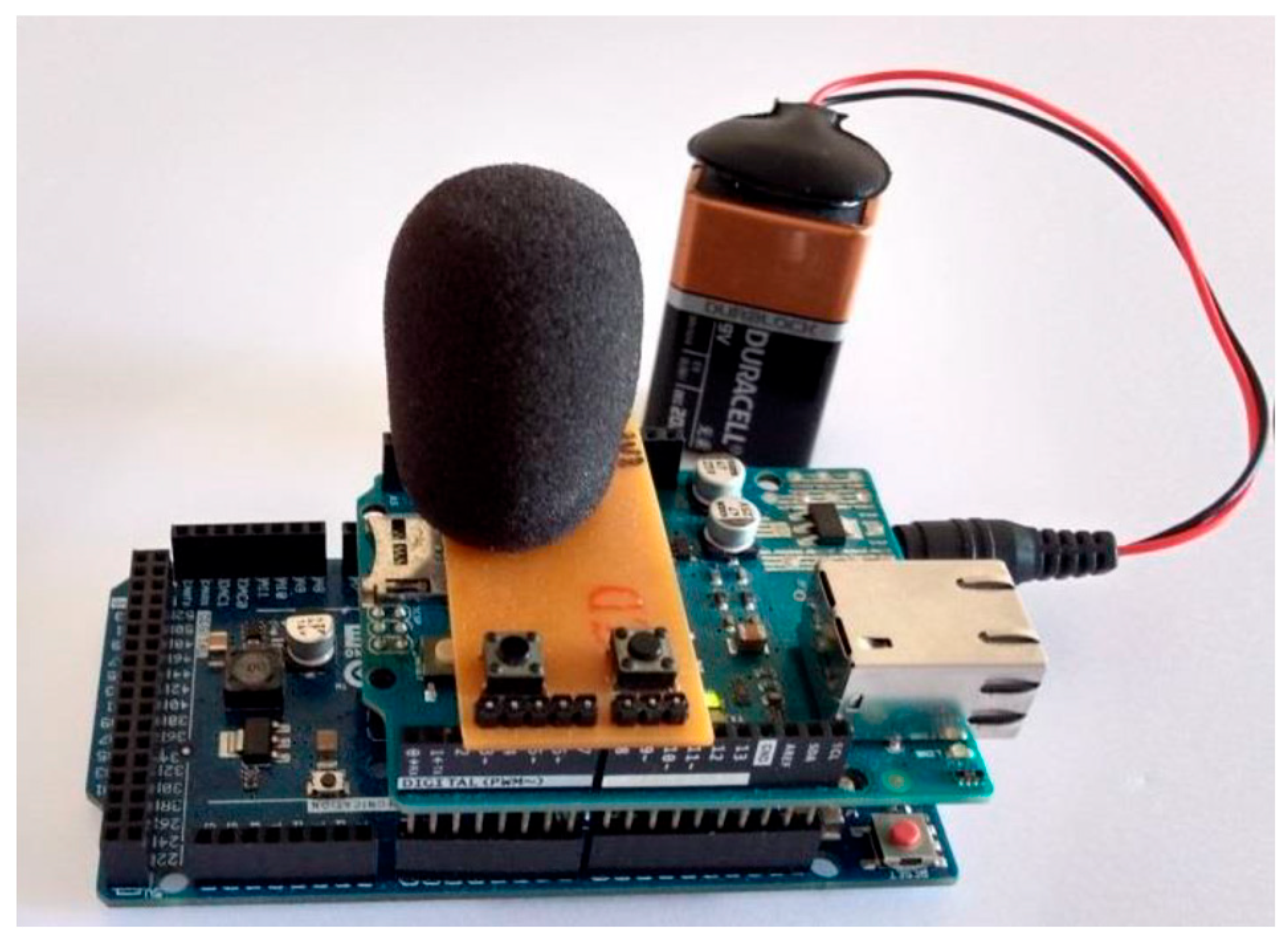
The data acquisition system (Figure 5) consisted of the following: (i) kit development board: responsible for interfacing and digitizing the signal; (ii) sensor module: a high-sensitivity electret microphone, calibrated for engine-noise characteristic frequencies; (iii) signal conditioning circuit: designed for amplification and basic filtering prior to digitization; (iv) USB interface for transferring raw data to a support laptop; and (v) acquisition software, developed in C/C++ and Python (version 3.12.11), responsible for controlling the sampling process and storing signals in WAVE format, with a 44.1 kHz sampling rate and 16-bit resolution, ensuring fidelity to the audible range and to typical mechanical and combustion fault frequencies [94]. In addition, during the tests, constant engine rotation and steady-state operating conditions were maintained to reduce external interferences and facilitate the identification of acoustic patterns [94].
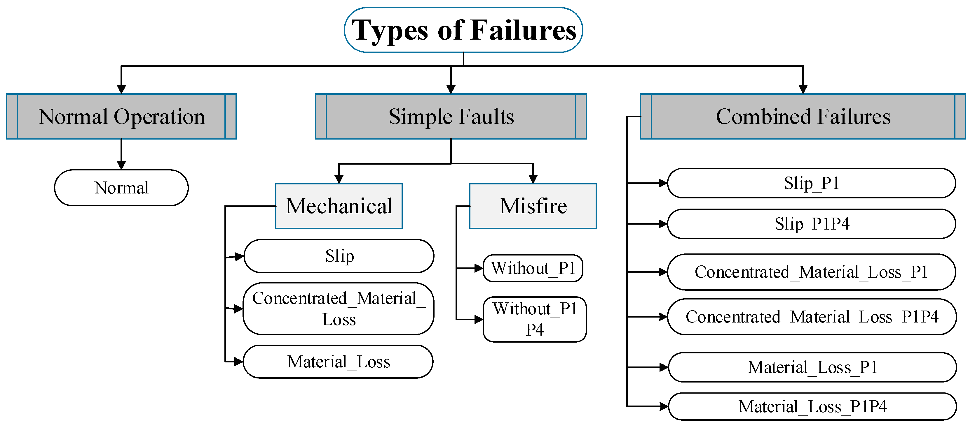
The faults were intentionally introduced into the engine following two main approaches: ignition faults: obtained by intentionally disconnecting spark plug wires, simulating combustion failures in one or more cylinders; mechanical faults: simulated through the controlled removal of alternator belt segments, generating slippage and material loss, which alter the dynamic behavior and produce distinctive sound patterns.
For each condition (normal, single faults, and combined faults), multiple acquisition cycles were performed. After data preprocessing, 12 fault subclasses were structured with 182 samples each, totaling 2184 samples, with each sample representing a 2 s time interval.
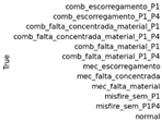
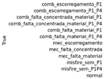
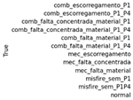
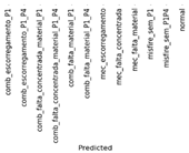
As shown in Figure 6, for simple belt faults there are three subclasses: slippage, concentrated material loss, and material loss. The term P1 indicates a fault in cylinder 1, and P1P4 indicates faults in two cylinders (P1 and P4). Finally, for combined faults, the term “Slippage P1” indicates a simultaneous belt slippage fault and misfire in cylinder 1, while “Slippage P1P4” indicates a combination of belt slippage with misfire faults in both cylinder P1 and cylinder P4, and so on for all other cases.
Although the experiments used a Ford Fiesta 1.6 (Otto cycle) dataset, the acoustic-signal-based diagnostic principles apply broadly to internal combustion engines (ICEs) in automotive, marine, and industrial contexts, as mechanical, ignition, and combustion failures share common thermodynamic and acoustic patterns.
The proposed deep-learning method can be adapted by adjusting the spectral range or resampling for different operating regimes. Data collected under controlled conditions with induced faults provide a robust reproducible basis for future studies, supporting data standardization and open research [48]. Suggested adaptations include the following: (i) acoustic scaling—adjust the sampling rate and STFT parameters for low-frequency content; (ii) spectral remapping—redefine mel-frequency bands for large-scale engines; (iii) order tracking—align acoustic frames with engine cycles to improve fault localization; and (iv) multimodal fusion—combine acoustic and vibration data to enhance robustness under maritime noise.
Experiments with a Ford Fiesta 1.6 (Otto cycle) dataset demonstrate that acoustic-signal-based diagnostics are broadly applicable to internal combustion engines (ICEs) across automotive, marine, and industrial contexts, as common thermodynamic and acoustic patterns underlie mechanical, ignition, and combustion faults. The deep-learning framework can be adapted by tuning the spectral parameters, remapping the frequency bands, applying order tracking, and integrating vibration data. Retraining is required for new operational contexts. Future work will extend the method to larger ICEs and marine applications, supported by a dedicated open dataset to advance predictive maintenance.

3.2. Experimental Setup and Instrumentation

The tools and technologies employed comprised a cloud-based computational environment on Google Colaboratory, equipped with hardware infrastructure featuring Graphics Processing Units (GPUs) compatible with the Compute Unified Device Architecture (CUDA) standard, enabling the efficient training of ML and DL models. The main libraries used for model development and evaluation were PyTorch (version 2.8.0+cu126), Optuna (version 4.5.0), Librosa (version 0.11.0), SoundFile (version 0.13.1), and Scikit-learn (version 1.6.1). For acoustic signal processing, the Librosa library was applied for reading audio files (.wav) and extracting log-mel spectrograms.
The experimental methodology adopted in this study was structured into a five-step pipeline (Figure 7), with the main characteristics described below.

3.2.1. Preprocessing of Input Data

This stage consisted of preprocessing the acoustic signals obtained from standardized audio files (.wav) of equal duration. Using the data augmentation technique [95], new audio samples with noise were added to the 12 fault subclasses of the dataset. Each subclass contained 182 samples, each with a duration of 2 s, totaling 2184 samples used for the evaluation of ML and DL models.

3.2.2. Feature Extraction with Log-Mel Spectrogram

In this step, for each 2 s audio file, a log-mel spectrogram was extracted as a representation of the acoustic features of the audio signals, with 64 frequency bands. The Short-Time Fourier Transform (STFT) was performed with a 1024-point FFT window, which determines the number of samples used to compute each frame, and a hop length of 256, representing the number of samples between consecutive frames.
The minimum and maximum frequency ranges were fixed at 20 Hz and 8000 Hz, respectively, preserving relevant spectro-temporal information of the acoustic signals. This representation is widely applied in classification tasks, as it converts raw audio into a visual representation that CNN, LSTM, GRU, BiGRUT, and Transformer models can process more effectively. Padding or truncation was applied to ensure that all spectrograms had exactly 124-time frames, providing dimensional uniformity for batch processing.

3.2.3. Data Partitioning

To ensure reproducibility, statistical robustness, and comparability across models, the dataset was stratified into three subsets: 70% for training and validation (with 20% of this portion reserved for validation) and 30% for testing. Stratified splitting by class guaranteed proportional representation of the 12 fault types in each subset, which is essential to prevent sampling bias, particularly in datasets with imbalanced classes [19].
Furthermore, the partitioning process was repeated three times for each model using random seeds with values of 42, 345, and 678, allowing multiple stratified split instances. This random-seed approach enabled the evaluation of model stability under different partitioning. Importantly, all ML and DL models were trained and evaluated with the same datasets in each run, ensuring identical experimental conditions and fair comparative validation.

3.2.4. Development, Training, and Evaluation

In this stage, the different ML (KNN, MLP, DT, GB, RF) and DL (LSTM, GRU, CNN, BiGRUT, Transformer) models were selected and implemented to classify the 12 fault types from ICE acoustic signals. Hyperparameter tuning for deep learning models (CNN, LSTM, GRU, Transformer, BiGRUT) was performed using Random Grid Search implemented via the Optuna framework [96]. Due to computational constraints, the search space was limited to 10 combinations per model. While this approach is common in machine learning, such a restriction may have contributed to the observed performance gap between the LSTM and GRU architectures, despite their structural similarities.
For each ML and DL architecture evaluated, specific parameter ranges were defined, including the hidden layer size, learning rate, number of epochs, batch size, and attention-related parameters (for Transformers). Model configurations were assessed based on validation set performance, ensuring generalization and mitigating the risk of overfitting. The hyperparameter combination achieving the best validation performance was then used to train each final model. The hyperparameters evaluated and applied in the ML and DL models are presented in Table 1.
It is important to note that each predictive model was evaluated over three runs with different random seeds, and the mean performance was used for assessment. Additionally, the same random seeds were applied across all evaluated models, ensuring a homogeneous data approach and enabling fair result comparisons.

3.2.5. Evaluation Metrics Analysis

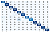
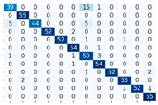
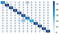
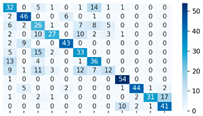
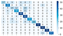
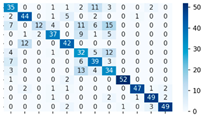
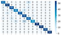
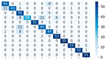
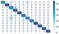
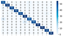
The trained architectures were evaluated on the test set with unseen data. Performance metrics analyzed included accuracy, precision, recall, F1-score, and MCC. In addition, confusion matrices were generated and used to provide insights into each model’s performance across different fault classes.

3.3. Proposed BiGRUT Hybrid Model

Based on the preliminary analysis of the evaluated ML and DL models, a new hybrid architecture was proposed, named BiGRUT, which combines Transformer attention mechanisms with bidirectional GRUs, capable of capturing local temporal dependencies. This design aims to complementarily exploit the advantages of each approach.
GRUs are efficient in capturing short- and medium-term sequences but may face limitations in modeling very long dependencies due to gradient accumulation. On the other hand, Transformers demonstrate strong capability in identifying long-range patterns through self-attention mechanisms, but they tend to perform less effectively when data lack a coherent and well-defined temporal structure.
In the BiGRUT model, illustrated in Figure 8, the 2 s input audio signal is converted into a log-mel spectrogram in batches of 128 samples, where each sample is represented by 64 mel-cepstral coefficients across 126 audio time frames.
Next, the spectrogram data undergo reshaping and matrix transposition operations and are then fed into a linear projection layer that maps them into a higher-dimensional space, combined with positional encoding to preserve the temporal order of frames.
The Transformer layer, employing a multi-head attention architecture, processes the sequence to extract global contextual attention and capture long-range dependencies. The Transformer output is subsequently processed by a bidirectional GRU layer, which refines temporal patterns from the global representation, capturing both forward and backward dependencies within the sequence.
The final state of the bidirectional GRU is extracted and passed through a dropout layer to mitigate overfitting. The resulting features are then fed into a fully connected Feed Forward layer, which performs the final classification, producing class probabilities.
Thus, the integration of both approaches aims to leverage their complementary strengths: while the GRU organizes and condenses sequential information locally, the Transformer expands the contextual representation, highlighting the most relevant information within the audio signals.
In summary, the methodology described in this section provides a robust and reproducible foundation for comparing predictive models under realistic conditions. From the construction of a balanced labeled acoustic dataset to the integration of advanced architectures such as BiGRUT, each component of the pipeline is aligned with the goal of addressing complex ICE fault detection challenges. The evaluation of these models under controlled experimental conditions is presented in Section 4, where performance metrics and fault-specific analyses are discussed in depth.

4. Results and Discussion

This section presents the experimental results obtained through the application of various machine learning (ML) and deep learning (DL) models to the task of fault detection in internal combustion engines (ICE) using acoustic signals. The analysis is organized to compare model performance based on standard classification metrics, such as accuracy, precision, recall, F1-score, and MCC. Particular emphasis is given to the proposed BiGRUT architecture, evaluating its effectiveness in complex fault scenarios. The results are presented in a structured manner: first addressing the general performance, then analyzing the model behavior by fault type, and finally interpreting the architectural advantages that explain the observed outcomes.

4.1. New Dataset for Benchmarking

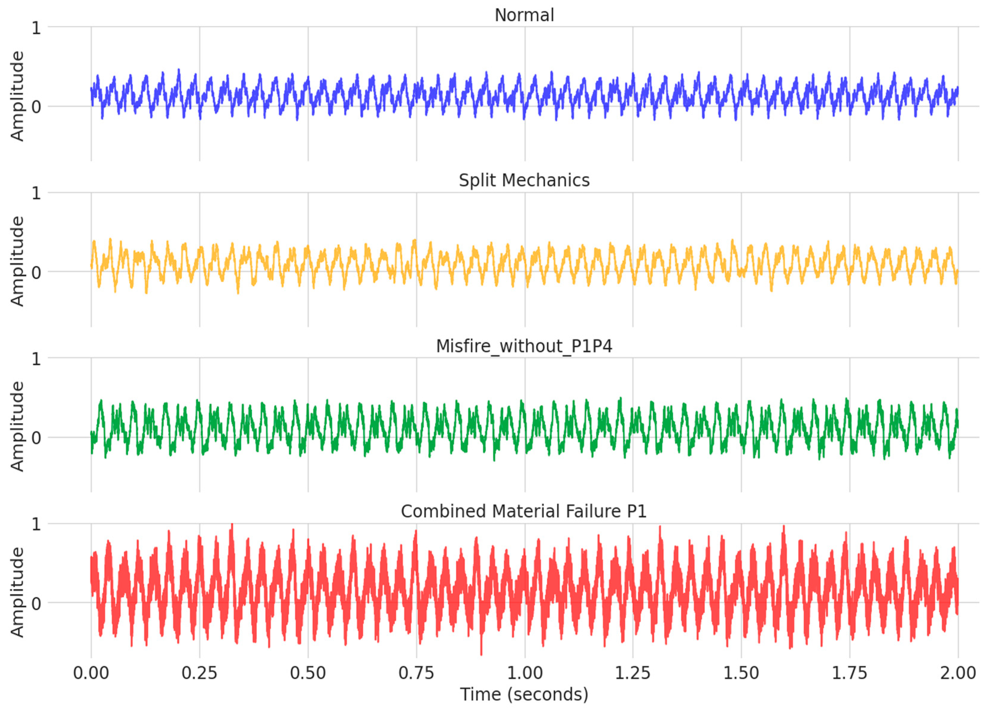
One of the key contributions of this study is the release of a new public, labeled, and structured dataset obtained under controlled experimental conditions. The dataset is composed of 12 fault subclasses (Figure 6), including normal operating conditions, mechanical faults, ignition faults, and combined faults, totaling 2184 samples. Each audio sample has a duration of 2 s at 16 kHz, preprocessed for the extraction of log-mel spectrograms with 64 filters and approximately 126 temporal frames. Figure 9 presents the temporal representation of audio signals under different engine operating conditions.
Unlike existing studies, which generally rely on proprietary or simulated data, the dataset provided in this study promotes transparency, reproducibility, and comparability across different approaches, thereby addressing a critical gap in the scientific literature of this field. As highlighted in the systematic review described in [48], no public, labeled, and standardized database with the comprehensiveness of 12 distinct fault subclasses was identified. Therefore, the dataset introduced here enables and fosters the development of new research in this area.
Moreover, the availability of a diversified and balanced real-world dataset allows for rigorous benchmarking of machine learning and deep learning architectures. Compared to datasets found in prior studies (often limited in scope, class variety, or accessibility) this dataset offers an open foundation for evaluating predictive models under realistic conditions. In the following subsections, the performance of the ML and DL models trained on this dataset is systematically analyzed and discussed.

4.2. Classification Performance by Metrics

The fault classification accuracy in ICEs was evaluated using five ML models (KNN, MLP, DT, GB, and RF) and five DL models (LSTM, GRU, Transformer, CNN, and the proposed BiGRUT). Table 2 presents the performance of the ML models across three runs (seeds), including the mean and standard deviation for all metrics. It was observed that the ANN-MLP model achieved the best overall performance across all evaluated metrics, with an average accuracy of 87.4%, proving to be a strong alternative for ICE fault detection. Possibly, as a neural-based structure for more robust DL models, MLP is capable of better capturing fault patterns in temporal data. As a shallow neural architecture, the MLP may leverage its inherent ability to generalize over moderate-sized datasets, which supports its relatively high performance.
The k-NN model also achieved competitive results, with a precision of 86.4% and a recall of 85.5%. As a distance-based classifier, it may have benefited from the stratified balancing of the dataset, making it a viable alternative with lower computational complexity compared to DL models. On the other hand, RF achieved higher accuracy (82.5%) than GB (74.3%), possibly due to GB’s sensitivity to noise or the need for more fine-tuned hyperparameter optimization. The poorest performance was obtained by the DT model, with an average accuracy of 52.9%.
Complementarily, Table 3 presents the results of the three runs for the DL models. It can be observed that BiGRUT and Transformer achieved the highest accuracy among all models, with mean accuracy values of 97.3% and 96.5%, respectively. This result suggests that the attention mechanism of the Transformer, when combined with the GRU’s capability to model long-term temporal dependencies, contributes significantly to the improvement in classification performance, particularly for acoustically complex fault patterns.
In contrast, the LSTM model achieved substantially lower accuracy (68.6%) compared to the other models. Given its functional and structural similarity to the GRU, this outcome may indicate the need for more extensive hyperparameter tuning or a broader exploration of parameter ranges beyond those tested in this study. One possible explanation is the limited hyperparameter search space adopted in our tuning process (10 combinations), which may have constrained the LSTM’s performance. Expanding this search could potentially reduce the observed gap, as LSTM architectures often require more fine-grained optimization to reach optimal performance for a given dataset and feature representation. Alternatively, the additional complexity of the LSTM—with its separate input, forget, and output gates—may not provide advantages under the specific conditions of our dataset size and temporal dependencies. In contrast, the GRU’s simpler gating mechanism appears to offer greater efficiency and stability, mitigating overfitting and gradient vanishing issues, which may account for its superior results.
Among the models with intermediate performance, CNN is noteworthy, achieving a precision of 94.2%. Although CNNs are primarily designed for image analysis—where spatial localization of features is critical—their use in this study proved reasonably effective for detecting localized patterns in spectrogram-based acoustic data.
When jointly evaluating ML and DL models, Figure 10a shows the mean accuracies and standard deviations from the three experimental runs. The results visually demonstrate that four out of the five DL models (CNN, GRU, BiGRUT, and Transformer) exhibit superior performance compared to ML models. In Figure 10b, the distribution, variability, median, and mean accuracies (%) of the ML and DL models are shown. Each point corresponds to the accuracy obtained in one seed-based execution used for data splitting. ML models displayed greater dispersion compared to DL models. The interquartile range (IQR), which reflects the statistical spread of central values within a dataset, was larger for ML models (IQR = 0.12) than for DL models (IQR = 0.08), indicating greater stability in the latter group.
Furthermore, the overall average accuracy of the DL models was superior, with values of 0.89 compared to 0.86 for ML models. These findings demonstrate the stronger classification capabilities of the evaluated DL architectures. The superior performance of DL models over ML is likely attributed to their ability to extract complex features and leverage long-term memory mechanisms. Moreover, the combination of architectures with attention mechanisms (Transformers) and recurrent networks with temporal memory (GRU) enables the development of hybrid models such as BiGRUT, which significantly enhanced the fault classification accuracy in ICEs.
In summary, the results presented in this subsection highlight the superior performance of deep learning models compared to traditional machine learning approaches in the task of ICE fault classification using acoustic signals. Among them, the proposed BiGRUT model consistently achieved the highest accuracy, demonstrating the benefits of combining sequential modeling with attention mechanisms. These findings support the growing applicability of DL-based systems for real-time predictive maintenance, especially in complex noise-prone environments. In the next subsection, a more granular analysis is conducted to evaluate how each model performs across specific fault subclasses, providing further insight into their strengths and limitations.

4.3. Performance Analysis by Fault Type

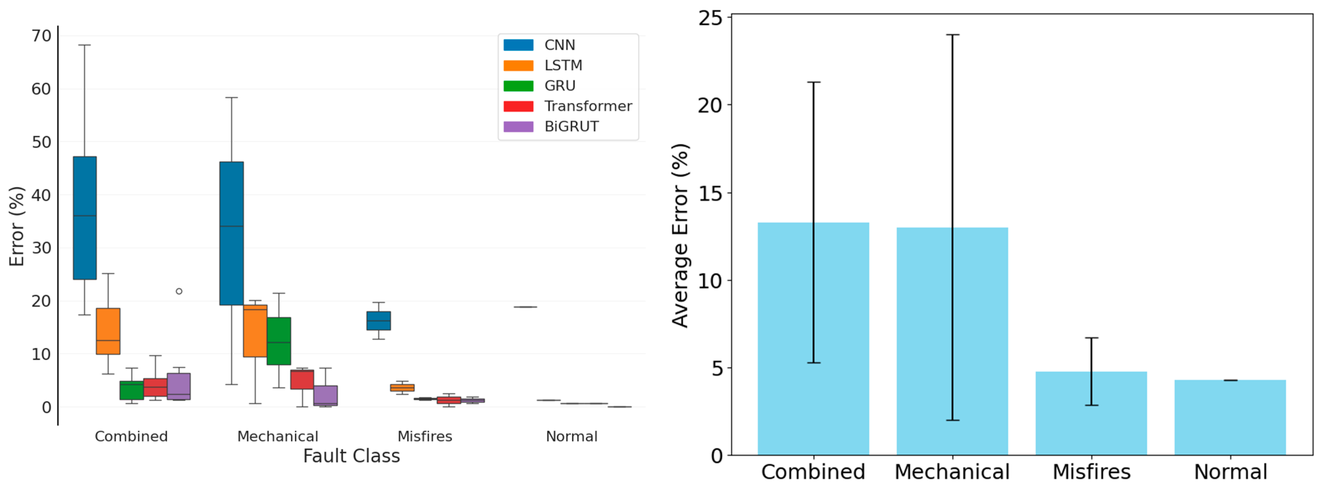
Based on the finding that DL models outperform ML models, this section presents an analysis of the fault detection performance by type of failure using the recall metric. As mentioned, recall represents the proportion of positive classes correctly identified by the model relative to the total number of actual positives. In other words, it reflects the model’s ability to correctly detect all relevant positive classes in the dataset. The complete data used in this analysis are shown in Table 4.
The analysis of detected and undetected classes and subclasses (Figure 11) highlights relevant differences in performance between models and failure types. For the normal (no fault) class processing 182.00 samples, Transformer achieved 0% error (no misclassifications), followed by BiGRUT and CNN with 0.6% (1104 misclassifications each), GRU with 1.22% (2226 errors), and LSTM with 18.9% incorrect classification (34,459 missed faults out of 182,000 samples). This demonstrates the feasibility of applying DL models to identify the presence or absence of ICE faults.
For misfires, analyzing 364 samples distributed across two subclasses, BiGRUT, Transformer, and CNN performed the best with errors below 2% (less than eight incorrect classifications each), while LSTM recorded an average error of 16.2% (59 undetected faults) in this category. This difference represents a reduction of approximately 51 critical undetected faults when comparing the best model versus LSTM.
The results indicate that fault detection in single cylinders is more effective than in multiple cylinders, as error rates nearly doubled in the latter case. In single-cylinder faults (182 samples), the top three models maintained error rates below 1.5% (less than three errors), while in two-cylinder faults, the rates rose to 2–3% (three–five incorrect classifications). This suggests that DL models are better able to capture the acoustic patterns of single-cylinder failures, while in two-cylinder failures, overlapping temporal patterns must be recognized, increasing the complexity of detection. Therefore, more effort should be directed toward the treatment of combined failures.
For mechanical faults, processing 546 samples covering three subclasses (182 samples each), BiGRUT and Transformer achieved the lowest error rates (2% and 4%, respectively, corresponding to 11 and 22 incorrect classifications). CNN and GRU, however, misclassified more than 12% of the samples (more than 65 errors each). Again, LSTM performed the worst with 32.26% error (176 undetected failures). This difference means that BiGRUT correctly detected 165 more failures than LSTM.
Considering that mechanical faults cover three different subclasses, it is observed that all the models exhibited higher error rates when the faults were grouped by similar origin. This is because belt-related faults can evolve from slippage to concentrated material loss. These subclasses often coexist or follow each other. However, among the models, BiGRUT achieved a maximum error rate of only 7.3% in mechanical failures (13 out of 182 samples), standing out as a promising alternative that, through the combination of self-attention and temporal memory mechanisms, can still be further optimized.
Similar to mechanical faults, combined faults also caused increased errors in BiGRUT, GRU, and LSTM. In contrast, Transformer maintained stable performance, while CNN showed reduced error compared to its performance on mechanical faults. Collectively, these results demonstrate that DL models tend to accumulate more errors when faults are combined or share the same mechanical origin. However, it is important to highlight that BiGRUT maintained a maximum error rate below 7.3% across all fault categories.
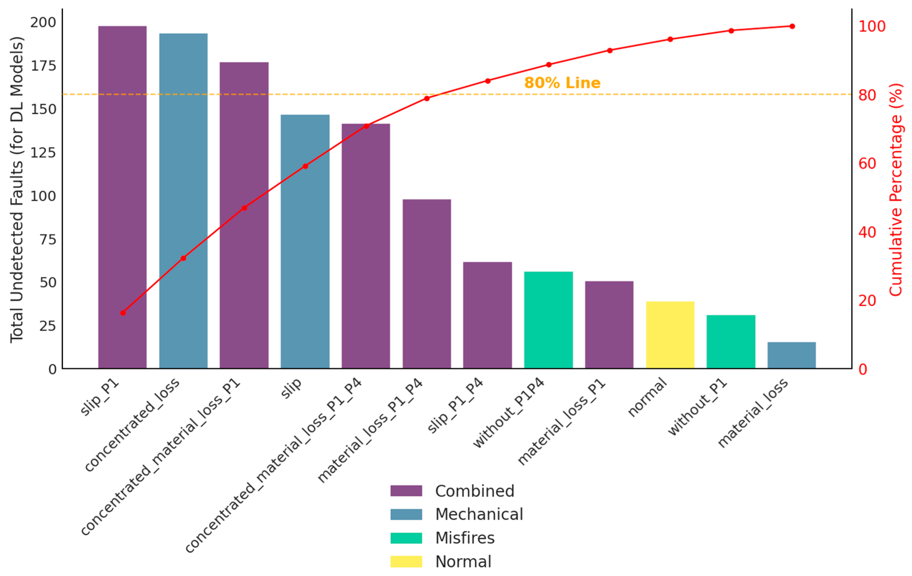
As illustrated in Figure 12, the most challenging cases for DL models were combined faults (e.g., Slippage P1) and mechanical faults due to concentrated material loss. Figure 12 clearly demonstrates that approximately 80% of undetected faults originated from only five subclasses (three combined and two mechanical), with the Slip_P1, Concentrated_loss, and Concentrated_material_loss_P1 classes alone accounting for about 50% of all undetected subclasses. These faults are complex to detect for all the evaluated algorithms due to their specific acoustic characteristics: combined faults exhibit spectral overlap from multiple simultaneous degradation mechanisms, while mechanical faults with concentrated material loss generate intermittent and non-stationary acoustic signatures that challenge conventional temporal pattern recognition.
The superior performance of the BiGRUT and Transformer architectures in handling these complex types of faults can be attributed to their advanced temporal modeling capabilities. BiGRUT combines bidirectional attention mechanisms with recurrent units, allowing it to capture both long-term temporal dependencies and complex local patterns characteristic of combined faults. Meanwhile, Transformer’s self-attention mechanisms excel at identifying nonlinear correlations between different spectral components that characterize mechanical failures with concentrated material loss.
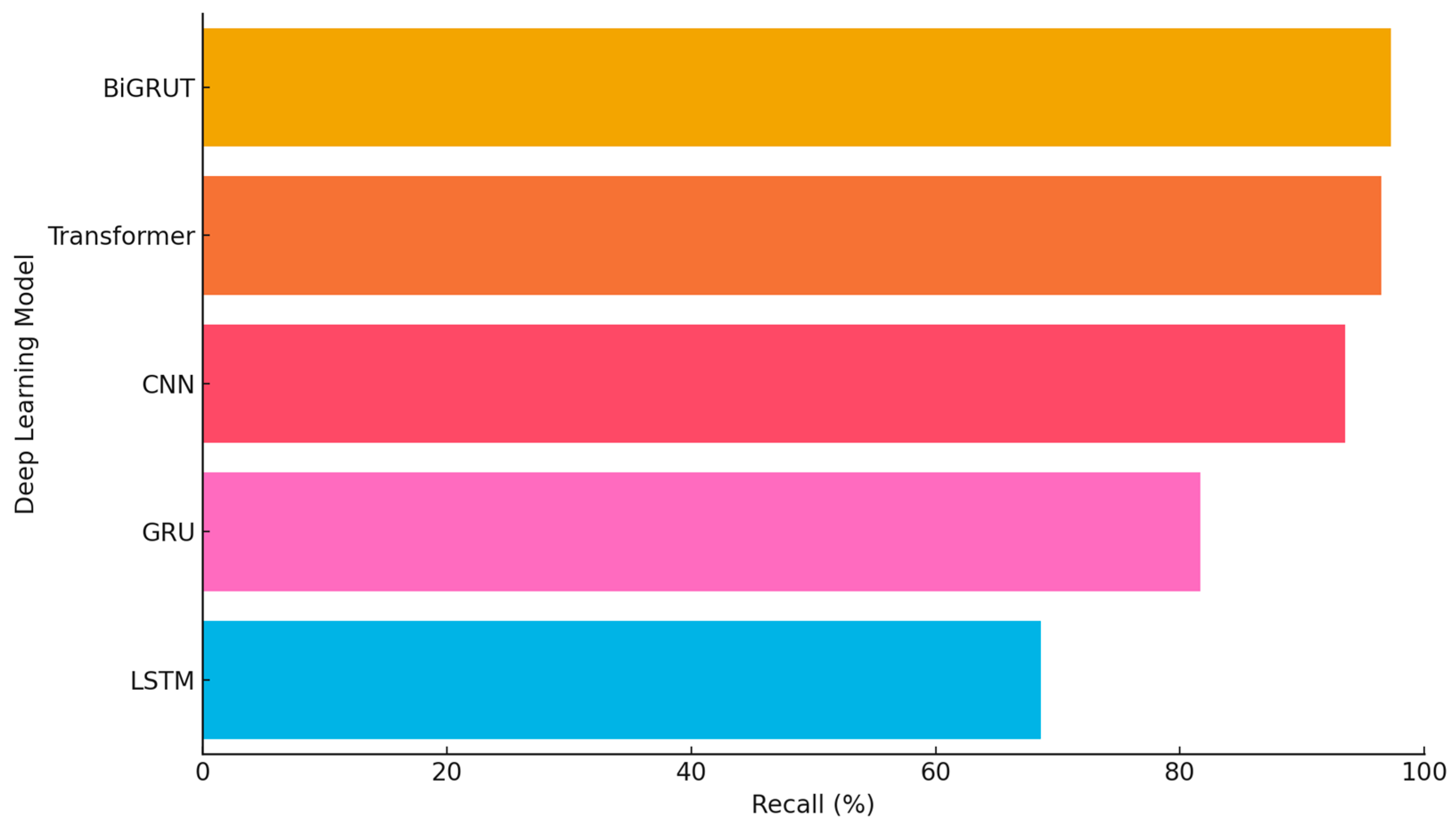
As quantitatively demonstrated in Figure 13, the proposed BiGRUT and Transformer proved to be the most effective approaches, achieving average correct detection rates of 97.3% and 96.5%, respectively, on the 182 fault samples per class—significantly outperforming CNN (93.5%), GRU (81.7%), and LSTM (68.6%).
Figure 14 provides a comparative summary of the average recall values for each evaluated Deep Learning model, visually reinforcing the quantitative analysis previously discussed. As observed, BiGRUT and Transformer lead with recall rates exceeding 96%, reflecting their superior ability to detect a broad spectrum of fault types with minimal error. CNN, while performing well overall, shows slightly lower effectiveness in complex failure modes, followed by GRU with a moderate drop in performance. LSTM, on the other hand, falls significantly behind, highlighting its limitations in modeling the non-linear and overlapping acoustic patterns present in ICE fault signals. This visual consolidation further validates the choice of hybrid and attention-based architectures as more suitable for real-world acoustic diagnostics in predictive maintenance systems.
Several studies have reported classification accuracies equal to or exceeding those obtained in this work. For instance, the authors of [50] employed a CNN architecture with acoustic data collected via smartphone, achieving up to 99.6% accuracy. However, direct comparison must be interpreted with caution due to key methodological differences: (i) the authors of [50] used a private dataset acquired under controlled conditions, whereas our dataset was collected in real operational environments; (ii) their classification task involved fewer fault categories, while our study addressed 12 subclasses, including combined and mechanical faults with overlapping spectral features; and (iii) our dataset is publicly available, enabling reproducibility and independent benchmarking, which is not the case for [50]. In summary, these findings highlight the need for greater focus on mechanical and combined faults. Furthermore, the adoption of more robust or additional filtering methods during the audio preprocessing stage, as well as the exploration of new hybrid classification approaches, may contribute to reducing errors in these fault categories.
In summary, these findings highlight the need for greater focus on mechanical and combined faults. Furthermore, the adoption of more robust or additional filtering methods during the audio preprocessing stage, as well as the exploration of new hybrid classification approaches, may contribute to reducing errors in these fault categories.
Overall, the results confirm the strong potential of deep learning models for non-invasive ICE fault detection, with BiGRUT demonstrating superior performance in nearly all evaluated scenarios. Its ability to combine long-range attention and sequential memory allowed for robust classification of both simple and complex fault patterns, especially in acoustically overlapping conditions. These outcomes validate the importance of hybrid architectures in handling real-world signal variability. Furthermore, the public and labeled dataset introduced in this study played a crucial role in enabling rigorous benchmarking and reproducibility. The findings reinforce the feasibility of scalable acoustic-based predictive maintenance systems and set the foundation for the concluding insights presented in Section 5.
This performance also reinforces the importance of selecting architectures that not only achieve high recall but also offer interpretability for real-world deployment. Understanding why certain models succeed or fail in specific fault subclasses can guide future improvements in signal preprocessing, feature extraction, and the design of advanced hybrid models.

5. Conclusions

This study successfully fulfilled its objective by proposing a novel approach and evaluating various Machine Learning (ML) and Deep Learning (DL) architectures for fault detection in internal combustion engines (ICEs) through acoustic signal analysis. The experiments demonstrated the superiority of DL models over traditional ML methods, particularly in more complex scenarios involving mechanical or combined faults. Among the evaluated models, the proposed hybrid architecture, BiGRUT, consistently outperformed others across multiple metrics, establishing itself as a promising solution for real-time non-invasive predictive maintenance.
The main contributions of this work are threefold. Methodologically, it introduces a publicly available, structured, and labeled dataset comprising 2184 samples across 12 ICE fault subclasses. Collected under controlled conditions and manually labeled, this dataset enables reproducibility and supports future advancements in the field. Experimentally, the study conducted a comprehensive comparative evaluation of ML and DL models using robust metrics—including accuracy, precision, recall, F1-score, and MCC—advancing the state of the art in acoustic-based fault classification. Practically, the findings validate the feasibility of low-cost, non-invasive, and efficient diagnostic systems for ICEs, with direct implications for reducing operational failures, maintenance expenses, and environmental impacts.
Despite its strengths, the study has some limitations. Experiments were conducted on a single automotive engine type with a fixed cylinder configuration, which limits the generalizability of the results. Future research should focus on validating BiGRUT in marine engines under dynamic operating conditions, exploring ensemble methods that integrate spectral and temporal features, and implementing the model in embedded platforms to assess performance in real-time inference scenarios.
Additionally, we intend to conduct a more in-depth investigation into the performance differences observed between the LSTM and GRU architectures.
When empirically compared to other study, the proposed BiGRUT model achieved an average accuracy of 97.3% across 12 fault subclasses, whereas study [50] addresses a smaller number of faults (three to five, depending on the scenario). Therefore, compared to prior works reporting higher accuracies under more controlled conditions and with fewer fault classes, our results demonstrate that BiGRUT delivers competitive performance in a more complex, realistic, and reproducible setting, reinforcing its value both as a predictive model and as a foundation for future research. This further highlights that BiGRUT can maintain high performance even in challenging classification scenarios, while contributing to the field through the provision of an open structured dataset for future investigations.
Although the experiments were conducted using an internal combustion engine (Ford Fiesta 1.6—Otto cycle), the diagnostic principles based on acoustic signals have broad applicability to ICEs in general, regardless of their application context (automotive, marine, or industrial). This is because mechanical, ignition, and combustion faults share common thermodynamic foundations and acoustic signatures. The adopted approach—based on deep learning and acoustic analysis—can be adapted to different operating conditions with minimal adjustments, such as spectral range calibration or resampling. Moreover, the use of real data obtained under controlled and fault-induced conditions provides a robust and reproducible foundation for future research. This reinforces the value of open datasets and encourages standardization in fault diagnosis systems. The work reported here is part of an ongoing research effort whose future phases will expand to larger ICEs with diverse operational characteristics, enabling the construction of broader diagnostic frameworks applicable across critical industries.
In summary, this research contributes to the advancement of predictive models based on artificial intelligence for fault diagnosis and predictive maintenance using sound waves. The results demonstrate the technical feasibility of applying the non-invasive method (sound waves) for fault detection. It is also noteworthy that the dataset and data preprocessing codes have been made available to the scientific community to enable further studies and ensure the reproducibility of the research (Open Source).
As a continuation of this research, we intend to advance the development of predictive models based on artificial intelligence, using acoustic and sound waves, and to explore how they can contribute to improving the performance of strategies for this application. Another avenue to be studied is the development of sensors and devices dedicated to acquiring signals for processing and analysis. One of the research areas to be further explored is the integration of energy harvesting-based systems, which would not only perform diagnostics but also promote improved energy efficiency and, consequently, reduce CO2 emissions [97,98,99,100,101,102,103,104,105,106]. This interdisciplinary approach aims at the technical and industrial development of the proposed solution for applicability and scalability, combining diagnosis and fault detection in ICEs with energy optimization, topics that are highly relevant for industrial applications and the large-scale transportation sector.

Author Contributions

Conceptualization: N.N.S.T., J.N.M., T.L.d.V.L., M.G., A.C.L.F., J.P.P.d.C. and O.H.A.J.; Methodology: N.N.S.T., J.N.M., T.L.d.V.L., M.G., A.C.L.F., J.P.P.d.C. and O.H.A.J.; Validation: N.N.S.T., J.N.M., T.L.d.V.L., M.G., A.C.L.F., J.P.P.d.C. and O.H.A.J.; Investigation and simulation: N.N.S.T., J.N.M. and O.H.A.J.; Writing—original draft preparation: N.N.S.T., J.N.M., and O.H.A.J.; Writing—review and editing: N.N.S.T., J.N.M., T.L.d.V.L., M.G., A.C.L.F., J.P.P.d.C. and O.H.A.J.; Project administration: J.N.M. and O.H.A.J. All authors have read and agreed to the published version of the manuscript.

Funding

This work was partially supported by the Brazilian National Council for Scientific and Technological Development (CNPq). This research was also partially supported by the FACEPE agency (Fundação de Amparo a Pesquisa de Pernambuco) through the project with the references APQ-0616-9.25/21 and APQ-0642-9.25/22. O.H.A.J. was funded by the Brazilian National Council for Scientific and Technological Development (CNPq), with the grant numbers 407531/2018-1, 303293/2020-9, 405385/2022-6, 405350/2022-8, and 40666/2022-3.

Data Availability Statement

The original contributions presented in this study are included in the article. Further inquiries can be directed to the corresponding author(s).

Conflicts of Interest

The authors declare no conflicts of interest.

Appendix A

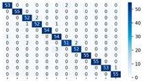
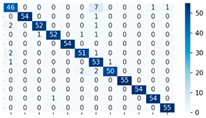
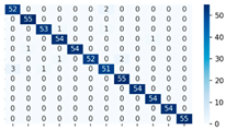
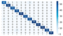
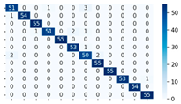
Table A1. Demonstration of the developed confusion matrix.
Seed 42Seed 456Seed 789
Asi 08 00147 i001Asi 08 00147 i002Asi 08 00147 i003Asi 08 00147 i004CNN
Asi 08 00147 i005Asi 08 00147 i006Asi 08 00147 i007Asi 08 00147 i008LSTM
Asi 08 00147 i009Asi 08 00147 i010Asi 08 00147 i011Asi 08 00147 i012GRU
Asi 08 00147 i013Asi 08 00147 i014Asi 08 00147 i015Asi 08 00147 i016Transformer
Asi 08 00147 i017Asi 08 00147 i018Asi 08 00147 i019Asi 08 00147 i020BiGRUT
Asi 08 00147 i021Asi 08 00147 i022Asi 08 00147 i023

References

  1. IEA; IRENA; UNSD; World Bank; WHO. Tracking SDG 7: The Energy Progress Report; WHO: Washington DC, USA, 2024; p. 179. [Google Scholar]
  2. Sachs, J.; Kroll, C.; Lafortune, G.; Fuller, G.; Woelm, F. Sustainable Development Report 2022, 1st ed.; Cambridge University Press: Cambridge, UK, 2022; ISBN 978-1-009-21005-8. [Google Scholar]
  3. CODS. Índice ODS 2022 Para América Latina y El Caribe; Centro de los Objetivos de Desarrollo Sostenible para América Latina y el Caribe: Bogotá, Colombia, 2023; p. 100. [Google Scholar]
  4. Ovrum, E.; Longva, T.; Leisner, M.; Bachmann, E.M.; Gundersen, O.S.; Helgesen, H.; Endresen, O. Energy Transition Outlook 2024—Maritime Forecast to 2050; DNV: Oslo, Norway, 2023; p. 73. [Google Scholar]
  5. United Nations Trade; Development (UNCTAD). Review of Maritime Transport 2024: Navigating Maritime Chokepoints, 1st ed.; Review of Maritime Transport Series; United Nations Research Institute for Social Development: Bloomfield, NJ, USA, 2024; ISBN 978-92-1-106592-3. [Google Scholar]
  6. Nahim, H.M.; Younes, R.; Nohra, C.; Ouladsine, M. Complete Modeling for Systems of a Marine Diesel Engine. J. Mar. Sci. Appl. 2015, 14, 93–104. [Google Scholar] [CrossRef]
  7. Neumann, S.; Varbanets, R.; Minchev, D.; Malchevsky, V.; Zalozh, V. Vibrodiagnostics of Marine Diesel Engines in IMES GmbH Systems. Ships Offshore Struct. 2023, 18, 1535–1546. [Google Scholar] [CrossRef]
  8. Dong, F.; Yang, J.; Cai, Y.; Xie, L. Transfer Learning-Based Fault Diagnosis Method for Marine Turbochargers. Actuators 2023, 12, 146. [Google Scholar] [CrossRef]
  9. Rodríguez, C.G.; Lamas, M.I.; Rodríguez, J.D.D.; Caccia, C. Analysis of the pre-injection configuration in a marine engine through several mcdm techniques. Brodogradnja 2021, 72, 1–17. [Google Scholar] [CrossRef]
  10. Varbanets, R.; Shumylo, O.; Marchenko, A.; Minchev, D.; Kyrnats, V.; Zalozh, V.; Aleksandrovska, N.; Brusnyk, R.; Volovyk, K. Concept of Vibroacoustic Diagnostics of the Fuel Injection and Electronic Cylinder Lubrication Systems of Marine Diesel Engines. Pol. Marit. Res. 2022, 29, 88–96. [Google Scholar] [CrossRef]
  11. Tharanga, K.L.P.; Liu, S.; Zhang, S.; Wang, Y. Diesel Engine Fault Diagnosis with Vibration Signal. J. Appl. Math. Phys. 2020, 8, 2031–2042. [Google Scholar] [CrossRef]
  12. Varbanets, R.; Fomin, O.; Píštěk, V.; Klymenko, V.; Minchev, D.; Khrulev, A.; Zalozh, V.; Kučera, P. Acoustic Method for Estimation of Marine Low-Speed Engine Turbocharger Parameters. J. Mar. Sci. Eng. 2021, 9, 321. [Google Scholar] [CrossRef]
  13. Deptuła, A.; Kunderman, D.; Osiński, P.; Radziwanowska, U.; Włostowski, R. Acoustic Diagnostics Applications in the Study of Technical Condition of Combustion Engine. Arch. Acoust. 2016, 41, 345–350. [Google Scholar] [CrossRef]
  14. Box, G.E.P.; Jenkins, G.M.; Reinsel, G.C.; Ljung, G.M. Time Series Analysis: Forecasting and Control, 5th ed.; Wiley Series in Probability and Statistics; John Wiley & Sons, Inc.: Hoboken, NJ, USA, 2016; ISBN 978-1-118-67502-1. [Google Scholar]
  15. Cooley, J.W.; Tukey, J.W. An Algorithm for the Machine Calculation of Complex Fourier Series. Math. Comput. 1965, 19, 297–301. [Google Scholar] [CrossRef]
  16. Karpenko, M.; Ževžikov, P.; Stosiak, M.; Skačkauskas, P.; Borucka, A.; Delembovskyi, M. Vibration Research on Centrifugal Loop Dryer Machines Used in Plastic Recycling Processes. Machines 2024, 12, 29. [Google Scholar] [CrossRef]
  17. Danilevičius, A.; Danilevičienė, I.; Karpenko, M.; Stosiak, M.; Skačkauskas, P. Determination of the Instantaneous Noise Level Using a Discrete Road Traffic Flow Method. Promet—Traffic Transp. 2025, 37, 71–85. [Google Scholar] [CrossRef]
  18. Espi, M.; Fujimoto, M.; Kinoshita, K.; Nakatani, T. Exploiting Spectro-Temporal Locality in Deep Learning Based Acoustic Event Detection. J. Audio Speech Music Process. 2015, 2015, 26. [Google Scholar] [CrossRef]
  19. Russell, S.J.; Norvig, P. Artificial Intelligence: A Modern Approach, 4th ed.; Pearson Series in Artificial Intelligence; Pearson: Hoboken, NJ, USA, 2020; ISBN 978-0-13-461099-3. [Google Scholar]
  20. Vaswani, A.; Shazeer, N.; Parmar, N.; Uszkoreit, J.; Jones, L.; Gomez, A.N.; Kaiser, Ł.; Polosukhin, I. Attention Is All You Need. In Proceedings of the Advances in Neural Information Processing Systems, Long Beach, CA, USA, 4–9 December 2017; Guyon, I., Luxburg, U.V., Bengio, S., Wallach, H., Fergus, R., Vishwanathan, S., Garnett, R., Eds.; Curran Associates, Inc.: New York, NY, USA, 2017; Volume 30. [Google Scholar]
  21. Abubakar, S.; Said, M.F.M.; Abas, M.A.; Samaila, U.; Ibrahim, A.A.; Ismail, N.A.; Narayan, S.; Kaisan, M.U. Application of artificial intelligence in internal combustion engines—Bibliometric analysis on progress and future research priorities. J. Balk. Tribol. Assoc. 2024, 30, 632–654. [Google Scholar]
  22. Ahmed, R.; El Sayed, M.; Gadsden, S.A.; Tjong, J.; Habibi, S. Automotive Internal-Combustion-Engine Fault Detection and Classification Using Artificial Neural Network Techniques. IEEE Trans. Veh. Technol. 2015, 64, 21–33. [Google Scholar] [CrossRef]
  23. Yang, M.; Chen, H.; Guan, C. Research on Diesel Engine Fault Diagnosis Method Based on Machine Learning. In Proceedings of the 2022 4th International Conference on Frontiers Technology of Information and Computer (ICFTIC), Qingdao, China, 2 December 2022; IEEE: Piscataway, NJ, USA; pp. 1078–1082. [Google Scholar]
  24. Czech, P.; Wojnar, G.; Burdzik, R.; Konieczny, Ł.; Warczek, J. Application of the Discrete Wavelet Transform and Probabilistic Neural Networks in IC Engine Fault Diagnostics. J. Vibroeng. 2014, 16, 1619–1639. [Google Scholar]
  25. Zheng, H.; Zhou, H.; Kang, C.; Liu, Z.; Dou, Z.; Liu, J.; Li, B.; Chen, Y. Modeling and Prediction for Diesel Performance Based on Deep Neural Network Combined with Virtual Sample. Sci. Rep. 2021, 11, 16709. [Google Scholar] [CrossRef] [PubMed]
  26. Makridis, G.; Kyriazis, D.; Plitsos, S. Predictive Maintenance Leveraging Machine Learning for Time-Series Forecasting in the Maritime Industry. In Proceedings of the 2020 IEEE 23rd International Conference on Intelligent Transportation Systems (ITSC), Rhodes, Greece, 20 September 2020; IEEE: Piscataway, NJ, USA, 2020; pp. 1–8. [Google Scholar]
  27. Xu, G.; Liu, M.; Jiang, Z.; Shen, W.; Huang, C. Online Fault Diagnosis Method Based on Transfer Convolutional Neural Networks. IEEE Trans. Instrum. Meas. 2020, 69, 509–520. [Google Scholar] [CrossRef]
  28. Senemmar, S.; Zhang, J. Deep Learning-Based Fault Detection, Classification, and Locating in Shipboard Power Systems. In Proceedings of the 2021 IEEE Electric Ship Technologies Symposium (ESTS), Arlington, VA, USA, 3 August 2021; IEEE: Piscataway, NJ, USA; pp. 1–6. [Google Scholar]
  29. Theodoropoulos, P.; Spandonidis, C.C.; Fassois, S. Use of Convolutional Neural Networks for Vessel Performance Optimization and Safety Enhancement. Ocean. Eng. 2022, 248, 110771. [Google Scholar] [CrossRef]
  30. Spandonidis, C.; Paraskevopoulos, D. Evaluation of a Deep Learning-Based Index for Prognosis of a Vessel’s Propeller-Hull Degradation. Sensors 2023, 23, 8956. [Google Scholar] [CrossRef]
  31. Laurie, A.; Anderlini, E.; Dietz, J.; Thomas, G. Machine Learning for Shaft Power Prediction and Analysis of Fouling Related Performance Deterioration. Ocean. Eng. 2021, 234, 108886. [Google Scholar] [CrossRef]
  32. Venkata, S.K.; Rao, S. Fault Detection of a Flow Control Valve Using Vibration Analysis and Support Vector Machine. Electronics 2019, 8, 1062. [Google Scholar] [CrossRef]
  33. Ellefsen, A.L.; Bjorlykhaug, E.; Aesoy, V.; Zhang, H. An Unsupervised Reconstruction-Based Fault Detection Algorithm for Maritime Components. IEEE Access 2019, 7, 16101–16109. [Google Scholar] [CrossRef]
  34. Ellefsen, A.L.; Cheng, X.; Holmeset, F.T.; Asoy, V.; Zhang, H.; Ushakov, S. Automatic Fault Detection for Marine Diesel Engine Degradation in Autonomous Ferry Crossing Operation. In Proceedings of the 2019 IEEE International Conference on Mechatronics and Automation (ICMA), Tianjin, China, 4–7 August 2019; IEEE: Piscataway, NJ, USA, 2019; pp. 2195–2200. [Google Scholar]
  35. Ellefsen, A.L.; Han, P.; Cheng, X.; Holmeset, F.T.; Aesoy, V.; Zhang, H. Online Fault Detection in Autonomous Ferries: Using Fault-Type Independent Spectral Anomaly Detection. IEEE Trans. Instrum. Meas. 2020, 69, 8216–8225. [Google Scholar] [CrossRef]
  36. Korczewski, Z. Test Method for Determining the Chemical Emissions of a Marine Diesel Engine Exhaust in Operation. Pol. Marit. Res. 2021, 28, 76–87. [Google Scholar] [CrossRef]
  37. Bogdanowicz, A.; Kniaziewicz, T. Marine Diesel Engine Exhaust Emissions Measured in Ship’s Dynamic Operating Conditions. Sensors 2020, 20, 6589. [Google Scholar] [CrossRef]
  38. Rodrigues, N.F.; Brito, A.V.; Ramos, J.G.G.S.; Mishina, K.D.V.; Belo, F.A.; Lima Filho, A.C. Misfire Detection in Automotive Engines Using a Smartphone Through Wavelet and Chaos Analysis. Sensors 2022, 22, 5077. [Google Scholar] [CrossRef]
  39. Smart, E.; Grice, N.; Ma, H.; Garrity, D.; Brown, D. One Class Classification Based Anomaly Detection for Marine Engines. In Intelligent Systems: Theory, Research and Innovation in Applications; Jardim-Goncalves, R., Sgurev, V., Jotsov, V., Kacprzyk, J., Eds.; Studies in Computational Intelligence; Springer International Publishing: Cham, Switzerland, 2020; Volume 864, pp. 223–245. ISBN 978-3-030-38703-7. [Google Scholar]
  40. Wieclawski, K.; Figlus, T.; Mączak, J.; Szczurowski, K. Method of Fuel Injector Diagnosis Based on Analysis of Current Quantities. Sensors 2022, 22, 6735. [Google Scholar] [CrossRef]
  41. Tamura, M.; Saito, H.; Murata, Y.; Kokubu, K.; Morimoto, S. Misfire Detection on Internal Combustion Engines Using Exhaust Gas Temperature with Low Sampling Rate. Appl. Therm. Eng. 2011, 31, 4125–4131. [Google Scholar] [CrossRef]
  42. Avan, E.Y.; Mills, R.; Dwyer-Joyce, R. Ultrasonic Imaging of the Piston Ring Oil Film During Operation in a Motored Engine—Towards Oil Film Thickness Measurement. SAE Int. J. Fuels Lubr. 2010, 3, 786–793. [Google Scholar] [CrossRef]
  43. Stoumpos, S.; Theotokatos, G.; Mavrelos, C.; Boulougouris, E. Towards Marine Dual Fuel Engines Digital Twins—Integrated Modelling of Thermodynamic Processes and Control System Functions. J. Mar. Sci. Eng. 2020, 8, 200. [Google Scholar] [CrossRef]
  44. Stoumpos, S.; Theotokatos, G. A Novel Methodology for Marine Dual Fuel Engines Sensors Diagnostics and Health Management. Int. J. Engine Res. 2022, 23, 974–994. [Google Scholar] [CrossRef]
  45. Aghazadeh Ardebili, A.; Ficarella, A.; Longo, A.; Khalil, A.; Khalil, S. Hybrid Turbo-Shaft Engine Digital Twining for Autonomous Air-Crafts via AI and Synthetic Data Generation. Aerospace 2023, 10, 683. [Google Scholar] [CrossRef]
  46. Wu, Z.; Li, J. A Framework of Dynamic Data Driven Digital Twin for Complex Engineering Products: The Example of Aircraft Engine Health Management. Procedia Manuf. 2021, 55, 139–146. [Google Scholar] [CrossRef]
  47. Jiang, J.; Li, H.; Mao, Z.; Liu, F.; Zhang, J.; Jiang, Z.; Li, H. A Digital Twin Auxiliary Approach Based on Adaptive Sparse Attention Network for Diesel Engine Fault Diagnosis. Sci. Rep. 2022, 12, 675. [Google Scholar] [CrossRef] [PubMed]
  48. Torres, N.N.S.; Lima, J.G.; Maciel, J.N.; Gazziro, M.; Filho, A.C.L.; Souto, C.R.; Salvadori, F.; Ando Junior, O.H. Non-Invasive Techniques for Monitoring and Fault Detection in Internal Combustion Engines: A Systematic Review. Energies 2024, 17, 6164. [Google Scholar] [CrossRef]
  49. Hountalas, T.D.; Founti, M.; Zannis, T.C. Experimental Investigation to Assess the Performance Characteristics of a Marine Two-Stroke Dual Fuel Engine Under Diesel and Natural Gas Mode. Energies 2023, 16, 3551. [Google Scholar] [CrossRef]
  50. Lima, T.L.; Filho, A.C.L.; Belo, F.A.; Souto, F.V.; Silva, T.C.B.; Mishina, K.V.; Rodrigues, M.C. Noninvasive Methods for Fault Detection and Isolation in Internal Combustion Engines Based on Chaos Analysis. Sensors 2021, 21, 6925. [Google Scholar] [CrossRef] [PubMed]
  51. Terwilliger, A.M.; Siegel, J.E. Improving Misfire Fault Diagnosis with Cascading Architectures via Acoustic Vehicle Characterization. Sensors 2022, 22, 7736. [Google Scholar] [CrossRef]
  52. Chen, J.; Randall, R.B.; Feng, N.; Peeters, B.; Van der Auweraer, H. Automated Diagnostics of Internal Combustion Engines Using Vibration Simulation. In Proceedings of the ICSV20, Bangkok, Thailand, 7–11 July 2013. [Google Scholar]
  53. Mahdisoozani, H.; Mohsenizadeh, M.; Bahiraei, M.; Kasaeian, A.; Daneshvar, A.; Goodarzi, M.; Safaei, M.R. Performance Enhancement of Internal Combustion Engines Through Vibration Control: State of the Art and Challenges. Appl. Sci. 2019, 9, 406. [Google Scholar] [CrossRef]
  54. Barelli, L.; Bidini, G.; Buratti, C.; Mariani, R. Diagnosis of Internal Combustion Engine Through Vibration and Acoustic Pressure Non-Intrusive Measurements. Appl. Therm. Eng. 2009, 29, 1707–1713. [Google Scholar] [CrossRef]
  55. Hwang, O.; Lee, M.C.; Weng, W.; Zhang, Y.; Li, Z. Development of Novel Ultrasonic Temperature Measurement Technology for Combustion Gas as a Potential Indicator of Combustion Instability Diagnostics. Appl. Therm. Eng. 2019, 159, 113905. [Google Scholar] [CrossRef]
  56. Förster, F.; Crua, C.; Davy, M.; Ewart, P. Temperature Measurements under Diesel Engine Conditions Using Laser Induced Grating Spectroscopy. Combust. Flame 2019, 199, 249–257. [Google Scholar] [CrossRef]
  57. Liang, J.; Mao, Z.; Liu, F.; Kong, X.; Zhang, J.; Jiang, Z. Multi-Sensor Signals Multi-Scale Fusion Method for Fault Detection of High-Speed and High-Power Diesel Engine under Variable Operating Conditions. Eng. Appl. Artif. Intell. 2023, 126, 106912. [Google Scholar] [CrossRef]
  58. Janiesch, C.; Zschech, P.; Heinrich, K. Machine Learning and Deep Learning. Electron Mark. 2021, 31, 685–695. [Google Scholar] [CrossRef]
  59. Hutter, F.; Kotthoff, L.; Vanschoren, J. (Eds.) Automated Machine Learning: Methods, Systems, Challenges; The Springer Series on Challenges in Machine Learning; Springer International Publishing: Cham, Switzerland, 2019; ISBN 978-3-030-05317-8. [Google Scholar]
  60. Quinlan, J.R. Induction of Decision Trees. Mach. Learn. 1986, 1, 81–106. [Google Scholar] [CrossRef]
  61. Lecun, Y.; Bengio, Y.; Hinton, G. Deep Learning. Nature 2015, 521, 436–444. [Google Scholar] [CrossRef]
  62. Elman, J.L. Finding Structure in Time. Cogn. Sci. 1990, 14, 179–211. [Google Scholar] [CrossRef]
  63. Bengio, Y.; Simard, P.; Frasconi, P. Learning Long-Term Dependencies with Gradient Descent Is Difficult. IEEE Trans. Neural Netw. 1994, 5, 157–166. [Google Scholar] [CrossRef]
  64. Pascanu, R.; Mikolov, T.; Bengio, Y. On the Difficulty of Training Recurrent Neural Networks. In Proceedings of the 30th International Conference on Machine Learning, Atlanta, GA, USA, 16–21 June 2013; Sanjoy, D., David, M., Eds.; Volume 28, pp. 1310–1318. [Google Scholar]
  65. Hochreiter, S.; Schmidhuber, J. Long Short-Term Memory. Neural Comput. 1997, 9, 1735–1780. [Google Scholar] [CrossRef]
  66. Mienye, I.D.; Swart, T.G.; Obaido, G. Recurrent Neural Networks: A Comprehensive Review of Architectures, Variants, and Applications. Information 2024, 15, 517. [Google Scholar] [CrossRef]
  67. Sit, M.; Demiray, B.Z.; Xiang, Z.; Ewing, G.J.; Sermet, Y.; Demir, I. A Comprehensive Review of Deep Learning Applications in Hydrology and Water Resources. Water Sci. Technol. 2020, 82, 2635–2670. [Google Scholar] [CrossRef]
  68. Perumal, T.; Mustapha, N.; Mohamed, R.; Shiri, F.M. A Comprehensive Overview and Comparative Analysis on Deep Learning Models. J. Artif. Intell. 2024, 6, 301–360. [Google Scholar] [CrossRef]
  69. Massaoudi, M.; Abu-Rub, H.; Refaat, S.S.; Chihi, I.; Oueslati, F.S. Deep Learning in Smart Grid Technology: A Review of Recent Advancements and Future Prospects. IEEE Access 2021, 9, 54558–54578. [Google Scholar] [CrossRef]
  70. Cho, K.; van Merrienboer, B.; Bahdanau, D.; Bengio, Y. On the Properties of Neural Machine Translation: Encoder-Decoder Approaches. arXiv 2014, arXiv:1409.1259. [Google Scholar] [CrossRef]
  71. Zhang, W.; Li, H.; Tang, L.; Gu, X.; Wang, L.; Wang, L. Displacement Prediction of Jiuxianping Landslide Using Gated Recurrent Unit (GRU) Networks. Acta Geotech. 2022, 17, 1367–1382. [Google Scholar] [CrossRef]
  72. Mateus, B.C.; Mendes, M.; Farinha, J.T.; Assis, R.; Cardoso, A.M. Comparing LSTM and GRU Models to Predict the Condition of a Pulp Paper Press. Energies 2021, 14, 6958. [Google Scholar] [CrossRef]
  73. Albawi, S.; Mohammed, T.A.; Al-Zawi, S. Understanding of a Convolutional Neural Network. In Proceedings of the 2017 International Conference on Engineering and Technology (ICET), Antalya, Turkey, 21–23 August 2017; IEEE: Piscataway, NJ, USA, 2017; pp. 1–6. [Google Scholar]
  74. LeCun, Y.; Bottou, L.; Bengio, Y.; Ha, P. Gradient-Based Learning Applied to Document Recognition. Proc. IEEE 1998, 86, 2278–2324. [Google Scholar] [CrossRef]
  75. Sandler, M.; Howard, A.; Zhu, M.; Zhmoginov, A.; Chen, L.-C. MobileNetV2: Inverted Residuals and Linear Bottlenecks. In Proceedings of the 2018 IEEE/CVF Conference on Computer Vision and Pattern Recognition, Salt Lake City, UT, USA, 18–22 June 2018; IEEE: Piscataway, NJ, USA, 2018; pp. 4510–4520. [Google Scholar]
  76. Iandola, F.N.; Han, S.; Moskewicz, M.W.; Ashraf, K.; Dally, W.J.; Keutzer, K. SqueezeNet: AlexNet-Level Accuracy with 50x Fewer Parameters and <0.5MB Model Size. arXiv 2016, arXiv:1602.07360. [Google Scholar]
  77. Liu, Y.; Wu, L. Intrusion Detection Model Based on Improved Transformer. Appl. Sci. 2023, 13, 6251. [Google Scholar] [CrossRef]
  78. He, K.; Zhang, X.; Ren, S.; Sun, J. Deep Residual Learning for Image Recognition. In Proceedings of the 2016 IEEE Conference on Computer Vision and Pattern Recognition (CVPR), Las Vegas, NV, USA, 26 June–1 July 2016; IEEE: Piscataway, NJ, USA, 2016; pp. 770–778. [Google Scholar]
  79. Ba, J.L.; Kiros, J.R.; Hinton, G.E. Layer Normalization. arXiv 2016, arXiv:1607.06450. [Google Scholar] [CrossRef]
  80. Gavrilyuk, K.; Sanford, R.; Javan, M.; Snoek, C.G.M. Actor-Transformers for Group Activity Recognition. In Proceedings of the IEEE/CVF Conference on Computer Vision and Pattern Recognition, Seattle, WA, USA, 13–19 June 2020. [Google Scholar]
  81. Zhuang, B.; Liu, J.; Pan, Z.; He, H.; Weng, Y.; Shen, C. A Survey on Efficient Training of Transformers. In Proceedings of the Proceedings of the Thirty-Second International Joint Conference on Artificial Intelligence, Macau, China, 19 August 2023; International Joint Conferences on Artificial Intelligence Organization: Stanford, CA, USA, 2023; pp. 6823–6831. [Google Scholar]
  82. Park, J.; Choi, K.; Jeon, S.; Kim, D.; Park, J. A Bi-Directional Transformer for Musical Chord Recognition. arXiv 2019, arXiv:1907.02698. [Google Scholar] [CrossRef]
  83. Goodfellow, I.; Bengio, Y.; Courville, A. Deep Learning (Adaptive Computation and Machine Learning); The MIT Press: Cambridge, UK, 2016; ISBN 978-0-262-03561-3. [Google Scholar]
  84. Haibo, H.; Garcia, E.A. Learning from Imbalanced Data. IEEE Trans. Knowl. Data Eng. 2009, 21, 1263–1284. [Google Scholar] [CrossRef]
  85. Chicco, D.; Jurman, G. The Advantages of the Matthews Correlation Coefficient (MCC) over F1 Score and Accuracy in Binary Classification Evaluation. BMC Genom. 2020, 21, 6. [Google Scholar] [CrossRef]
  86. Teodoro, L.D.A.; Kappel, M.A.A. Aplicação de Técnicas de Aprendizado de Máquina Para Predição de Risco de Evasão Escolar Em Instituições Públicas de Ensino Superior No Brasil. Rev. Bras. Inform. Educ. 2020, 28, 838–863. [Google Scholar] [CrossRef]
  87. Tharwat, A. Classification Assessment Methods. Appl. Comput. Inform. 2021, 17, 168–192. [Google Scholar] [CrossRef]
  88. Jain, D.; Singh, V. Feature Selection and Classification Systems for Chronic Disease Prediction: A Review. Egypt. Inform. J. 2018, 19, 179–189. [Google Scholar] [CrossRef]
  89. Guimaraes, M.T.; Medeiros, A.G.; Almeida, J.S.; Falcao, Y.; Martin, M.; Damasevicius, R.; Maskeliunas, R.; Cavalcante Mattos, C.L.; Reboucas Filho, P.P. An Optimized Approach to Huntington’s Disease Detecting via Audio Signals Processing with Dimensionality Reduction. In Proceedings of the 2020 International Joint Conference on Neural Networks (IJCNN), Glasgow, UK, 19–24 July 2020; IEEE: Piscataway, NJ, USA, 2020; pp. 1–8. [Google Scholar]
  90. Medeiros, T.A.; Saraiva Junior, R.G.; Cassia, G.D.S.E.; Nascimento, F.A.D.O.; Carvalho, J.L.A.D. Classification of 1p/19q Status in Low-Grade Gliomas: Experiments with Radiomic Features and Ensemble-Based Machine Learning Methods. Braz. Arch. Biol. Technol. 2023, 66, e23230002. [Google Scholar] [CrossRef]
  91. Pająk, M.; Kluczyk, M.; Muślewski, Ł.; Lisjak, D.; Kolar, D. Ship Diesel Engine Fault Diagnosis Using Data Science and Machine Learning. Electronics 2023, 12, 3860. [Google Scholar] [CrossRef]
  92. Ranachowski, Z.; Bejger, A. Fault diagnostics of the fuel injection system of a medium power maritime diesel engine with application of acoustic signal. Arch. Acoust. 2005, 30, 465–472. [Google Scholar]
  93. Theodoropoulos, P.; Spandonidis, C.C.; Giannopoulos, F.; Fassois, S. A Deep Learning-Based Fault Detection Model for Optimization of Shipping Operations and Enhancement of Maritime Safety. Sensors 2021, 21, 5658. [Google Scholar] [CrossRef]
  94. de Lima, T.L.V.; Lima Filho, A.C. Métodos Não Invasivos Para Detecção E Isolamento De Falhas Em Motores De Combustão Interna Baseados Em Dimensões Fractais E Análise Multiresolução Wavelet. Ph.D. Thesis, Universidade Federal da Paraíba, Paraíba, Brasil, 2020. [Google Scholar]
  95. Iglesias, G.; Talavera, E.; González-Prieto, Á.; Mozo, A.; Gómez-Canaval, S. Data Augmentation Techniques in Time Series Domain: A Survey and Taxonomy. Neural Comput. Applic. 2023, 35, 10123–10145. [Google Scholar] [CrossRef]
  96. Yang, L.; Shami, A. On Hyperparameter Optimization of Machine Learning Algorithms: Theory and Practice. Neurocomputing 2020, 415, 295–316. [Google Scholar] [CrossRef]
  97. Ando Junior, O.H.; Maran, A.L.O.; Henao, N.C. A Review of the Development and Applications of Thermoelectric Microgenerators for Energy Harvesting. Renew. Sustain. Energy Rev. 2018, 91, 376–393. [Google Scholar] [CrossRef]
  98. Ando Junior, O.H.; Calderon, N.H.; De Souza, S.S. Characterization of a Thermoelectric Generator (TEG) System for Waste Heat Recovery. Energies 2018, 11, 1555. [Google Scholar] [CrossRef]
  99. Ando Junior, O.H.; Izidoro, C.L.; Gomes, J.M.; Correia, J.H.; Carmo, J.P.; Schaeffer, L. Acquisition and Monitoring System for TEG Characterization. Int. J. Distrib. Sens. Netw. 2015, 11, 531516. [Google Scholar] [CrossRef]
  100. Calderón-Henao, N.; Venturini, O.J.; Franco, E.H.M.; Eduardo Silva Lora, E.; Scherer, H.F.; Maya, D.M.Y.; Ando Junior, O.H. Numerical–Experimental Performance Assessment of a Non-Concentrating Solar Thermoelectric Generator (STEG) Operating in the Southern Hemisphere. Energies 2020, 13, 2666. [Google Scholar] [CrossRef]
  101. Izidoro, C.L.; Ando Junior, O.H.; Carmo, J.P.; Schaeffer, L. Characterization of Thermoelectric Generator for Energy Harvesting. Measurement 2017, 106, 283–290. [Google Scholar] [CrossRef]
  102. Kramer, L.R.; Maran, A.L.O.; De Souza, S.S.; Ando Junior, O.H. Analytical and Numerical Study for the Determination of a Thermoelectric Generator’s Internal Resistance. Energies 2019, 12, 3053. [Google Scholar] [CrossRef]
  103. Maran, A.L.O.; Henao, N.C.; Silva, E.A.; Schaeffer, L.; Ando Junior, O.H. Use of the Seebeck Effect for Energy Harvesting. IEEE Lat. Am. Trans. 2016, 14, 4106–4114. [Google Scholar] [CrossRef]
  104. Silva, E.A.D.; Filho, W.M.C.; Cavallari, M.R.; Ando Junior, O.H. Self-Powered System Development with Organic Photovoltaic (OPV) for Energy Harvesting from Indoor Lighting. Electronics 2024, 13, 2518. [Google Scholar] [CrossRef]
  105. Silva, E.; Urzagasti, C.; Maciel, J.; Ledesma, J.; Cavallari, M.; Ando Junior, O.H. Development of a Self-Calibrated Embedded System for Energy Management in Low Voltage. Energies 2022, 15, 8707. [Google Scholar] [CrossRef]
  106. Sylvestrin, G.R.; Scherer, H.F.; Ando Junior, O.H. Hardware and Software Development of an Open Source Battery Management System. IEEE Lat. Am. Trans. 2021, 19, 1153–1163. [Google Scholar] [CrossRef]
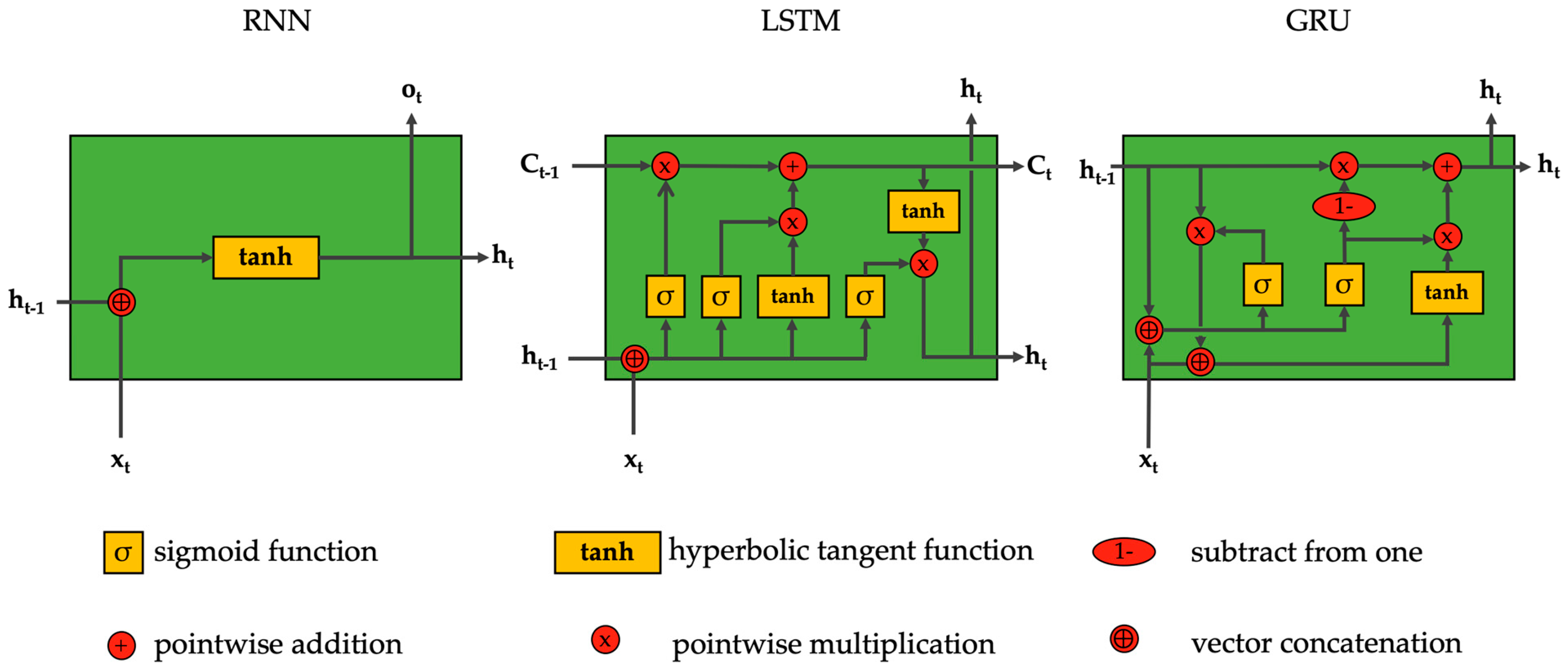
Figure 1. Computation comparison of RNN, LSTM and GRU nodes [67].
Asi 08 00147 g001
Figure 2. Architecture of LeNet-5, a Convolutional Neural Network, here for digits recognition. Source: Adapted from [74].
Asi 08 00147 g002
Figure 3. Architecture of the Transformer model [20].
Asi 08 00147 g003
Figure 4. Vehicle used for data capturing. Source: Prepared by the author.
Asi 08 00147 g004
Figure 5. Data acquisition system developed. Source: Prepared by the author.
Asi 08 00147 g005
Figure 6. Failure type flow diagram.
Asi 08 00147 g006
Figure 7. Phases of the pipeline developed.
Asi 08 00147 g007
Figure 8. Proposed BiGRUT architecture and stages.
Asi 08 00147 g008
Figure 9. Temporal representation of audio signals under different engine operating conditions.
Asi 08 00147 g009
Figure 10. Accuracies and means for all the evaluated models.
Asi 08 00147 g010
Figure 11. Error distribution by fault class and model.
Asi 08 00147 g011
Figure 12. Pareto analysis—undetected failures by type.
Asi 08 00147 g012
Figure 13. Total number of faults detected by model.
Asi 08 00147 g013
Figure 14. Average recall (%) for fault detection across deep learning models.
Asi 08 00147 g014
Table 1. Selected hyperparameters in evaluated ML and DL models.
Machine Learning
Hyperparameters SVC RF GB DT k-NN ANN-MLP
ScalerRobust ScalerStandard ScalerRobust Scaler--Robust Scaler
C/N Estimators/NeighborsC = 2.406464-5(64, 32)
Kernel/Criterionlinearlog2 (max_features)learning_rate = 0.001entropyp = 1logistic
Max Depth-108None--
Min Samples Split-555--
Min Samples Leaf-552--
Bootstrap/Subsample-False0.9---
Weights/Solver----distancelbfgs
Learning Rate/Alpha-----alpha = 0.001
Max Iter-----1000
Deep Learning
HyperparametersCNNLSTMGRUTransformerBiGRUT
Layers (1–3)3 (Conv2D)111 (Transformer Blocks)1 (Transf)/1 (LSTM)
Units/Layer (32, 64, 128, 256)32128128128128/128
Batch Size (64, 128)128128128128128
Dropout (0.0, 0.1, 0.2, 0.3)0.20.10.20.20.2
Epochs (20, 30)3030303030
Optimizer (Adam, SGD, RMSprop)AdamWAdamWAdamWAdamWAdamW
Sequence Length (2, 5)22222
Learning Rate (1 × 10⁻⁴–5 × 10⁻³)0.0010.00320.0010.0010.001
Activation Function (ReLU, tanh)ReLUTanh Tanh ReLUReLU + tanh
Convolutional Layers (1, 2, 3)3----
Kernel (3 × 3, 5 × 5)3 × 3----
Pooling (Max, Average)Max + Adaptive Avg----
Head Attention (2, 4)---44
Dimension Feed-forward Layer (32, 64, 128, 256)---128128
Table 2. Evaluation metrics for ML models.
ModelSeedMetrics
AccuracyPrecisionRecallF1-ScoreMCC
Decision Tree10.5150.5220.5150.5160.472
20.5210.5270.5210.5210.478
30.5500.5490.5440.5440.509
Mean0.5290.5330.5270.5270.486
Standard Deviation 0.0190.0140.0150.0150.020
Gradient
Boosting
10.7590.7650.7590.7530.739
20.7350.7470.7350.7340.712
30.7360.6880.6970.6870.713
Mean0.7430.7330.7300.7250.721
Standard Deviation 0.0140.0400.0310.0340.015
k-NN10.8660.8710.8660.8670.854
20.8510.8580.8500.8490.838
30.8560.8640.8480.8520.843
Mean0.8580.8640.8550.8560.845
Standard Deviation 0.0080.0070.0100.0100.008
ANN-MLP10.8800.8840.8800.8800.869
20.8580.8580.8580.8570.846
30.8830.8790.8770.8760.873
Mean0.8740.8740.8720.8710.863
Standard Deviation 0.0140.0140.0120.0120.015
Random Forest10.8090.8110.8090.8010.794
20.8280.8320.8270.8210.813
30.8380.8450.8170.8190.824
Mean0.8250.8290.8180.8140.810
Standard Deviation 0.0150.0170.0090.0110.015
Table 3. Evaluation metrics for DL models.
ModelSeedMetrics
AccuracyPrecisionRecallF1-ScoreMCC
CNN10.9500.9530.9500.9490.945
20.9330.9400.9330.9340.927
30.9240.9340.9240.9220.918
Mean0.9350.9420.9350.9350.930
Standard Deviation0.0130.0100.0130.0140.014
LSTM10.6480.6750.6480.6450.618
20.6910.6980.6900.6760.666
30.7200.7520.7200.7160.696
Mean0.6860.7080.6860.6790.660
Standard Deviation0.0360.0390.0360.0360.039
GRU10.8700.8750.8710.8700.859
20.8770.8940.8760.8750.867
30.9190.9260.9190.9200.912
Mean0.8890.8980.8890.8880.880
Standard Deviation0.0270.0260.0270.0270.029
Transformer10.9570.9590.9570.9570.954
20.9770.9770.9770.9770.975
30.9600.9630.9600.9610.957
Mean0.9650.9660.9650.9650.962
Standard Deviation0.0110.0100.0110.0110.012
BiGRUT
(proposed)
10.9800.9800.9800.9800.978
20.9600.9610.9600.9600.957
30.9770.9770.9770.9770.975
Mean0.9730.9730.9730.9730.970
Standard Deviation0.0110.0100.0110.0110.012
Table 4. Performance analysis by failure type of deep learning models.
ModelFault ClassFault SubclassRecall
Average
Faults
Detected
Undetected FaultsError (%)Average Error (%) Per Class
CNNCombinedSlip_P10.782142.29439.70621.8176.09 ± [8.05]
Slip_P1_P40.988179.7922.2081.213
Concentrated_material_loss_P10.926168.55613.4447.387
Concentrated_material_loss_P1_P40.988179.7552.2451.233
Material_loss_P10.982178.6333.3671.850
Material_loss_P1_P40.970176.4855.5153.030
MechanicalSlip0.878159.82022.18012.18712.43 ± [8.91]
Concentrated_loss0.785142.94339.05721.460
Material_loss0.964175.3816.6193.637
MisfiresWithout_P10.988179.7922.2081.2131.53 ± [0.45]
Without_P1P40.982178.6333.3671.850
NormalNormal0.994180.8961.1040.6070.607
LSTMCombinedSlip_P10.50992.65689.34449.09038.09 ± [18.98]
Slip_P1_P40.782142.29439.70621.817
Concentrated_material_loss_P10.31757.645124.35568.327
Concentrated_material_loss_P1_P40.585106.54375.45741.460
Material_loss_P10.827150.54431.45617.283
Material_loss_P1_P40.695126.39955.60130.550
MechanicalSlip0.659119.86562.13534.14032.26 ± [27.13]
Concentrated_loss0.41675.700106.30058.407
Material_loss0.958174.2837.7174.240
MisfiresWithout_P10.872158.69823.30212.80316.25 ± [4.87]
Without_P1P40.803146.17035.83019.687
NormalNormal0.811147.54134.45918.93318.933
GRUCombinedSlip_P10.794144.49637.50420.60714.33 ± [7.17]
Slip_P1_P40.909165.45616.5449.090
Concentrated_material_loss_P10.878159.85722.14312.167
Concentrated_material_loss_P1_P40.749136.26345.73725.130
Material_loss_P10.938170.76511.2356.173
Material_loss_P1_P40.872158.73423.26612.783
MechanicalSlip0.799145.41236.58820.10312.99 ± [10.77]
Concentrated_loss0.817148.74933.25118.270
Material_loss0.994180.8961.1040.607
MisfiresWithout_P10.976177.5834.4172.4273.67 ± [1.76]
Without_P1P40.951173.0528.9484.917
NormalNormal0.988179.7742.2261.2231.223
TransformerCombinedSlip_P10.903164.35217.6489.6974.26 ± [3.15]
Slip_P1_P40.988179.7922.2081.213
Concentrated_material_loss_P10.945172.0399.9615.473
Concentrated_material_loss_P1_P40.951173.1438.8574.867
Material_loss_P10.981178.6273.3731.853
Material_loss_P1_P40.975177.5234.4772.460
MechanicalSlip0.933169.76412.2366.7234.68 ± [4.06]
Concentrated_loss0.927168.68413.3167.317
Material_loss1.000182.0000.0000.000
MisfiresWithout_P11.000182.0000.0000.0001.23 ± [1.74]
Without_P1P40.975177.5294.4712.457
NormalNormal1.000182.0000.0000.0000
BiGRUT
(proposed)
CombinedSlip_P10.926168.60513.3957.3603.67 ± [2.66]
Slip_P1_P40.994180.8961.1040.607
Concentrated_material_loss_P10.963175.2966.7043.683
Concentrated_material_loss_P1_P40.951173.1128.8884.883
Material_loss_P10.994180.8961.1040.607
Material_loss_P1_P40.951173.1618.8394.857
MechanicalSlip0.927168.68413.3167.3172.64 ± [4.06]
Concentrated_loss0.994180.8961.1040.607
Material_loss1.000182.0000.0000.000
MisfiresWithout_P10.994180.8781.1220.6171.22 ± [0.85]
Without_P1P40.982178.6943.3061.817
NormalNormal0.994180.8961.1040.6070.607
Disclaimer/Publisher’s Note: The statements, opinions and data contained in all publications are solely those of the individual author(s) and contributor(s) and not of MDPI and/or the editor(s). MDPI and/or the editor(s) disclaim responsibility for any injury to people or property resulting from any ideas, methods, instructions or products referred to in the content.