Shear Strength Prediction for RCDBs Utilizing Data-Driven Machine Learning Approach: Enhanced CatBoost with SHAP and PDPs Analyses

Abstract

Reinforced concrete deep beams (RCDBs) provide significant strength and serviceability for building structures. However, a simple, general, and universally accepted procedure for predicting their shear strength (SS) has yet to be established. This study proposes a novel data-driven approach to predicting the SS of RCDBs using an enhanced CatBoost (CB) model. For this purpose, a newly comprehensive database of RCDBs with shear failure, including 950 experimental specimens, was established and adopted. The model was developed through a customized procedure including feature selection, data preprocessing, hyperparameter tuning, and model evaluation. The CB model was further evaluated against three data-driven models (e.g., Random Forest, Extra Trees, and AdaBoost) as well as three prominent mechanics-driven models (e.g., ACI 318, CSA A23.3, and EU2). Finally, the SHAP algorithm was employed for interpretation to increase the model’s reliability. The results revealed that the CB model yielded a superior accuracy and outperformed all other models. In addition, the interpretation results showed similar trends between the CB model and mechanics-driven models. The geometric dimensions and concrete properties are the most influential input features on the SS, followed by reinforcement properties. In which the SS can be significantly improved by increasing beam width and concert strength, and by reducing shear span-to-depth ratio. Thus, the proposed interpretable data-driven model has a high potential to be an alternative approach for design practice in structural engineering.

1. Introduction

Reinforced concrete deep beams (RCDBs) are structural elements characterized by their small shear span-to-depth ratio ($a/d$ approximately $\le 2.5$) and/or effective span-to-height ratio ($l_e/h<5$ in GB 50010, $l_e/h<4$ in ACI 318, and $l_e/h<3$ in EU2), thereby offering a greater load-carrying capacity than equivalent slender beams. For this reason, RCDBs are extensively utilized in large-scale projects such as bridges, high-rise buildings, and offshore structures. Nevertheless, due to the relatively small $a/d$ ratio, the ultimate load-carrying capacity is predominantly governed by shear behavior, which is difficult to model accurately compared to slender beams, as the theory of plane sections is not valid due to the nonlinear strain distributions [1]. Hence, the main question in the design and application of RCDBs revolves around how to accurately model and predict their shear strength (SS) to avoid catastrophic failure.

Since 1960, various approaches have been proposed to predict the SS of RCDBs. The most commonly adopted approach among those is the strut-and-tie model (STM) [2], which has been adopted by many codes of practice such as ACI 318, CSA A23.3, and EU2. STM represents a simplistic and powerful method that predominantly provides conservative strength predictions. The other approaches have also shown reasonable strength predictions for a limited set of experimental tests. However, the shear resisting mechanism of RCDBs is more complicated as it is governed by several complex behaviors, such as size effects, dowel actions, and bond-slip effects of tensile reinforcements, aggregate interlock at crack interfaces, shear transverse reinforcement effect, flexure-shear interaction, etc., as shown in Figure 1. Hence, all these behaviors are difficult to capture in a unique model using theoretical approaches, which makes the model unstable and may result in inaccurate predictions. Moreover, adopting these traditional approaches requires some assumptions and simplifications, time-consuming calibration processes, as well as being mostly complicated for practical implementation. These limitations have motivated structural engineers toward dealing with advanced soft computing techniques, which can provide a promising alternative.

With rapid development in artificial intelligence, data-driven approaches such as machine learning (ML) are capable of solving and overcoming the aforementioned limitations. Accordingly, ML approaches have been successfully applied to predict the SS of RCDBs. For example, an early ML application was made by Sanad and Saka [3] using an ANN algorithm with a database of 111 specimens and 10 input parameters. Pal and Deswal [4] examined the potential of the SVR algorithm in predicting the SS of RCDBs, considering a database of 106 specimens and 9 input variables. Mohammadhassani et al. [5] employed the ANFIS algorithm with a database of 139 specimens to build their predictive model for RCDBs. Chou et al. [6] proposed a hybrid predictive model using an LS-SVR algorithm coupled with SFA. A database of 214 specimens and 9 input features was used to calibrate their model. Shahnewaz et al. [7] developed an improved predictive model for RCDBs by adopting a genetic algorithm. Their predictive model was calibrated utilizing a database of 381 specimens and 8 input parameters. Prayogo et al. [8] developed a new predictive model, namely OSVM-AEW, by combining SVM and LS-SVM with SOS algorithms. The model was constructed using 214 samples and 7 input parameters.

Recently, Feng et al. [9] adopted four ensemble ML algorithms, namely RF, AdaBoost, GBRT, and XGBoost, to develop predictive models for SS of RCDBs. For this purpose, a database of 271 specimens and 16 input variables was used in calibration. The results showed that the XGBoost model has a superior performance over all other models. Truong et al. [10] adopted the XGBoost algorithm coupled with Bayesian optimization to develop a hybrid predictive model, namely BO-XGBoost. This model was built considering a database of 320 specimens and demonstrated high performance. In addition, Ma et al. [11] considered six ML algorithms, namely KNN, DT, RF, GBRT, XGBoost, and CatBoost. The predictive models were built considering a database of 457 specimens and 9 input features. The results also indicated that the XGBoost model outperformed all other models. Nguyen et al. [12] adopted seven ML algorithms, namely LR, ANN, SVR, DT, EoT, XGBoost, and GPR. Then, predictive models for SS of RCDBs were constructed using data from 518 specimens and 15 input parameters. It was demonstrated that GPR is the most accurate model. Moreover, Tiwari et al. [13] suggested eight ML-based predictive models (e.g., ANN, DT, SVR, RF, GBRT, XGBoost, AdaBoost, and VR) based on a database of 271 samples and 16 input variables. It was revealed that XGBoost outperformed all other models in prediction.

Although these ML models have achieved variable levels of accuracy in predicting the SS of RCDBs, there are several shortcomings that still need to be addressed. Firstly, most previous studies were carried out on a limited number of specimens and features, which imposed restrictions on the performance of ML. Hence, it is vital to expand the database to obtain more reliable and robust predictive models. Secondly, some of the above studies [3,4,5,6,7,8] were carried out using individual ML algorithms, which lack the generalization ability and model interpretability. Thirdly, there is significant confusion in selecting the effective and appropriate ML algorithms, which is typically the most crucial phase that must be dealt with at the initial stage. Several studies [9,10,13] demonstrated that XGBoost performed best, while others [3] indicated that different ML models, like ANN, can provide highly accurate results. On the other hand, the study by [12] showed that GPR is the most accurate model for prediction. This contradiction demands a comprehensive evaluation of various ML models in predicting the SS for RCDBs to provide a shortcut for practicing engineers. Fourthly, only a few studies have examined the model interpretability and transparency related to the shear mechanism of RCDBs.

In view of the above, there is a critical need for more comprehensive, accurate, reliable, and practical ML models for predicting the SS of RCDBs. Therefore, the main research objective of this study is to present a novel data-driven predictive approach using an enhanced CatBoost model and incorporating a large database compilation to address the aforementioned shortcomings and concerns. The study further hypothesizes that the CatBoost model can outperform existing models in predicting the SS of RCDBs. Accordingly, the contribution of this study can be clarified as follows: (1) establishing a comprehensive experimental database consisting of 950 shear tests conducted on RCDBs with different web reinforcements. This could further encourage the researchers to adopt the data-driven approach in this field; (2) developing a unified predictive ML model suited for four types of RCDBs and then being evaluated against existing conventional (mechanics-driven) models. This can solve a traditional problem in structural engineering and hence provide an alternative approach for design practices; (3) employing the SHAP and PDPs analyses to investigate the importance and impact of various input features on the CatBoost model prediction in terms of interpretation. The result could assist in designing RCDBs by achieving the desired SS within a few trials, hence saving time, cost, labor, and materials.

2. Materials and Methods

2.1. Experimental Database of RCDBs

2.1.1. Database Description

This research presents a comprehensive database of 950 experimental specimens of RCDBs failed in shear, collected from 69 earlier publications published between 1951 and 2024 [14,15,16,17,18,19,20,21,22,23,24,25,26,27,28,29,30,31,32,33,34,35,36,37,38,39,40,41,42,43,44,45,46,47,48,49,50,51,52,53,54,55,56,57,58,59,60,61,62,63,64,65,66,67,68,69,70,71,72,73,74,75,76,77,78,79,80,81,82]. These specimens were selected based on the following criteria:

• Specimens with only rectangular cross-sections were considered (a/d ≤ 2.5).
• Specimens were cast using low to high-strength concrete.
• Specimens with different web reinforcements were considered.
• Specimens with only deformed steel bars were considered (no limit on yield strength).
• Specimens were tested under three-point or four-point or monotonic loads.
• Specimens with axial or prestressed or post-tensioned loading were not considered.
• Specimen’s ultimate shear strength is less than 2000 kN.
• Specimens with only adequate information were recorded.

Based on web reinforcement, the database includes four different types of RCDBs: 412 WOR (RCDBs without reinforcement), 42 WHR (RCDBs with horizontal reinforcement), 268 WVR (RCDBs with vertical reinforcement), and 228 WHVR (RCDBs with horizontal and vertical reinforcement) (see Figure 2).

2.1.2. Feature Selection

According to numerous experimental and theoretical investigations, the shear strength in RCDBs is governed by different key factors such as concrete properties, geometrical dimensions, and longitudinal and web reinforcement characteristics. Hence, 16 important features were selected and defined as the input parameters, and thus categorized as follows: (1) concrete property: compressive strength ($f_c^{\prime }$); (2) geometric dimensions: width ($b$), beam span ($l_e$), height ($h$), shear span ($a$), beam depth ($d$), effective span-to-height proportion ($l_e/h$), and shear span-to-depth proportion ($a/d$); (3) longitudinal steel: steel percentage (${\rho }_l$) and strength ($f_{yl}$); (4) horizontal web reinforcement: steel percentage (${\rho }_h$), space ($s_h$), and strength ($f_{yh}$); (5) vertical web reinforcement: steel percentage (${\rho }_v$), space ($s_v$), and strength ($f_{yv}$). The experimental shear strength ($V_u,Exp.$) was set as the corresponding output parameter. Earlier investigations [83,84] indicated that the size of the database ought to exceed ten times of number of input parameters. Therefore, this study meets the basic requirements for utilizing machine learning in regression problems.

Table 1. Overview of the selected features incorporated in the database.

Category	Feature	Type	Unit	Min	Max	Mean	SD	Skew	Kurtosis
Concrete property	$f_c^{\prime }$	Input	MPa	11.30	120.10	41.67	21.40	0.88	−0.14
Geometric dimension	$b$	Input	mm	51.00	600.00	172.89	85.24	1.45	2.58
	$l_e$	Input	mm	300.00	6400.00	1623.63	855.16	1.55	3.91
	$h$	Input	mm	152.00	1829.00	522.30	252.32	1.97	5.32
	$a$	Input	mm	102.00	2625.00	577.50	402.52	2.36	7.04
	$d$	Input	mm	132.00	1778.00	463.67	233.02	1.97	5.35
	$l_0/h$	Input	-	0.91	5.85	3.24	1.17	0.20	−0.49
	$a/d$	Input	-	0.22	2.74	1.29	0.58	0.49	−0.47
Longitudinal reinforcement	${\rho }_l$	Input	%	0.00	11.27	1.89	1.09	1.59	7.27
	$f_{yl}$	Input	MPa	0.00	1330.00	455.25	150.00	1.54	7.53
Horizontal web reinforcement	${\rho }_h$	Input	%	0.00	3.17	0.17	0.42	3.86	17.60
	$s_h$	Input	mm	0.00	801.00	46.57	99.87	3.11	11.62
	$f_{yh}$	Input	MPa	0.00	860.00	127.33	211.46	1.28	0.26
Vertical web reinforcement	${\rho }_v$	Input	%	0.00	2.86	0.27	0.41	2.51	8.65
	$s_v$	Input	mm	0.00	457.00	87.97	108.11	1.12	0.33
	$f_{yv}$	Input	MPa	0.00	1051.00	224.69	232.69	0.47	−0.65
Shear strength	$V_u,Exp.$	Output	kN	21.00	1984.50	411.15	332.60	1.98	4.43

provides a comprehensive overview of the selected features incorporated in the database, outlining their type, measurement units, and statistical information (min, max, mean, standard deviation (SD), etc.). Figure 3 illustrates the plots of the statistical information, offering significant insights. In which the horizontal axes represent the selected features, and the vertical axes refer to the number of specimens in the database. In general, the established database exhibits a broad spectrum and diversity, enhancing ML models to have superior generalization abilities.

2.1.3. Preprocessing of Database

For ML modeling, preprocessing steps should be carried out after feature selection. First, a normalization process for input features is usually conducted to avoid scale effects, specifically when some features in the database vary widely. In this study, the normalization was conducted by scaling the input features to the range of [0, 1] using the MinMaxScaler method. Second, after normalization, ML modeling also requires splitting the database into datasets for the training and testing processes. The training dataset will be used to develop a prediction model for each algorithm. The testing dataset is then used to evaluate the accuracy of each ML model in predicting the SS. Accordingly, a total of 950 specimens were randomly split into 80% for the training process and 20% for the testing process, as recommended by most previous studies.

2.2. Overview of Selected ML Algorithms

Over the last three decades, several ML algorithms have been developed, and it is confusing which algorithm to adopt. Each has benefits and drawbacks and was designed for a specific application. Recently, the CatBoost algorithm has caught widespread attention due to its proven excellent performance across various regression and classification tasks. Nonetheless, its application to RCDBs is quite limited in comparison to other tree-based algorithms, as evidenced by the literature. Thus, CatBoost was adopted as the primary algorithm in this research to build a data-driven predictive model for the SS of RCDBs. Three well-known ML algorithms, such as Random Forest, Extra Trees, and AdaBoost, were also adopted for comparison with the CatBoost model. The predictive models were built and coded using Colab Notebooks environment with Python 3 and scikit-learn library. The selected algorithms are briefly described in following subsections.

2.2.1. Random Forest (RF)

RF is a supervised ML algorithm devised by Breiman in 2001 and belongs to the ensemble learning family. RF constructs a forest of DT predictors as weak learners during training using the bootstrap sampling technique (bagging) in a parallel manner to produce a final prediction, as shown in Figure 4. The basic concept of this technique is that each DT is trained on a bootstrap sampling (random sampling with replacement) from the original dataset, and during construction, a random subset of features is considered at each split, hence introducing diversity among the DTs [85,86]. For a dataset $D={\left\{\left(x_i, y_i\right)\right\}}_{i=1}^N$, the RF prediction for an input $x$ is given by:

$$F\left(x\right)={\displaystyle \frac{1}{T}}\sum _{t=1}^T{f}_t(x)$$

(1)

where $f_t\left(x\right)$ is the prediction from $t^{th}$ DT and $t=1,\dots ,T$ is the number of DTs in the forest.

2.2.2. Extra Trees (ET)

ET, or extremely randomized trees, is a supervised ML algorithm devised by Geurts et al. in 2006 [87] and belongs to the ensemble learning family. ET also constructs a forest of DT predictors as weak learners during training, similar to the RF algorithm but with a high level of randomness. Rather than using the bootstrap sampling technique, each DT predictor is typically trained using the whole training dataset but maintains randomness through selecting cut-points at random for feature splits. The high level of randomness in ET tends to reduce variance and hence improve generalization performance, especially on noisy data [88,89]. Formally, the final prediction from an ET model is given by:

$$F\left(x\right)={\displaystyle \frac{1}{T}}\sum _{t=1}^T{f}_t^{extra}(x)$$

(2)

where $f_t^{extra}(x)$ represents the prediction from an individual extremely randomized DT.

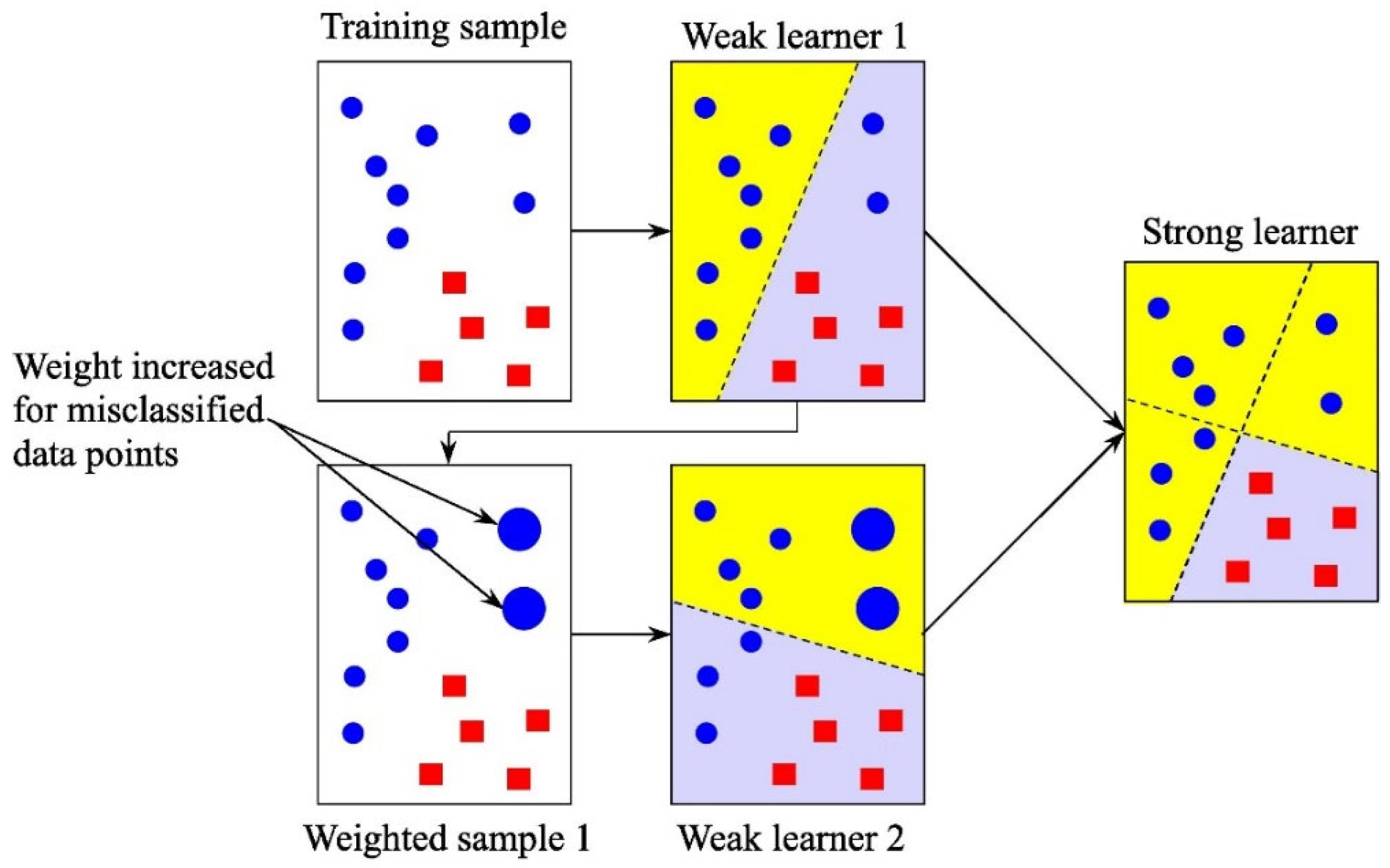
2.2.3. AdaBoost (AB)

AB is one of the ensemble boosting algorithms, which has received increasing attention due to its good performance in solving practical problems. The primary idea behind AB is to train weak learners like DTs in an iterative way (see Figure 5). In each iteration, the iterative process is completed by initially assigning weights to each sample and then updating its weights. This means that during each iteration, a new learner will evaluate the weighting coefficient. The weight will be increased for the sample that was poorly predicted by the previous learner, while the weight of correctly predicted specimen will be decreased. In the meantime, the exponential loss will enable the sum of training errors to be minimized. Finally, AB builds a strong single learner through integrating multiple weak learners [9].

$$F\left(x\right)=\sum _{t=1}^T{\alpha }_t{f}_t(x)$$

(3)

where $f_t\left(x\right)$ is the $t^{th}$ weak learner, ${\alpha }_t={\displaystyle \frac{1}{2}}\mathit{ln}\left({\displaystyle \frac{1-{\epsilon }_t}{{\epsilon }_t}}\right)$, and ${\epsilon }_t$ is the weighted error of the $t^{th}$ learner.

2.2.4. CatBoost (CB)

CB is a supervised ML algorithm devised by Prokhorenkova et al. in 2018 [90] and belongs to the ensemble learning family. It is a powerful open-source boosting tree algorithm that can handle a wide range of data science problems. CB employs several procedures to improve its performance, precision, and computing efficiency. For instance, it deals with categorical features instead of data normalization or transformation during the boosting process considering the whole training dataset. Also, it adopts a novel technique using a gradient descent algorithm to determine the loss function and the best splits while building the DTs sequentially. Moreover, it utilizes a regularization term to reduce overfitting risks and hence improves model generalizability [91]. The objective function of the CB which combines the loss function and regularization terms can be identified in Equation (4).

$$Obj=\sum _{i=1}^{N}L\left({\widehat{y}}_i,y_i\right)+\sum _{t=1}^T\Omega \left(f_t\right)$$

(4)

where $L$ is the loss function, $i=1,\dots ,N$ is the number of specimens, ${\widehat{y}}_i$ and $y_i$ are predicted and actual values of $i^{th}$ specimens, respectively, $\Omega \left(f_t\right)=$ the regularization term, $t=1,\dots ,T$ is the number of DTs.

The final prediction of CB is obtained from aggregating the predictions of the individual DTs scaled by the learning rate η as indicated in Equation (5) [92].

$$F\left(x\right)=\sum _{t=1}^T\eta F_t\left(x\right)$$

(5)

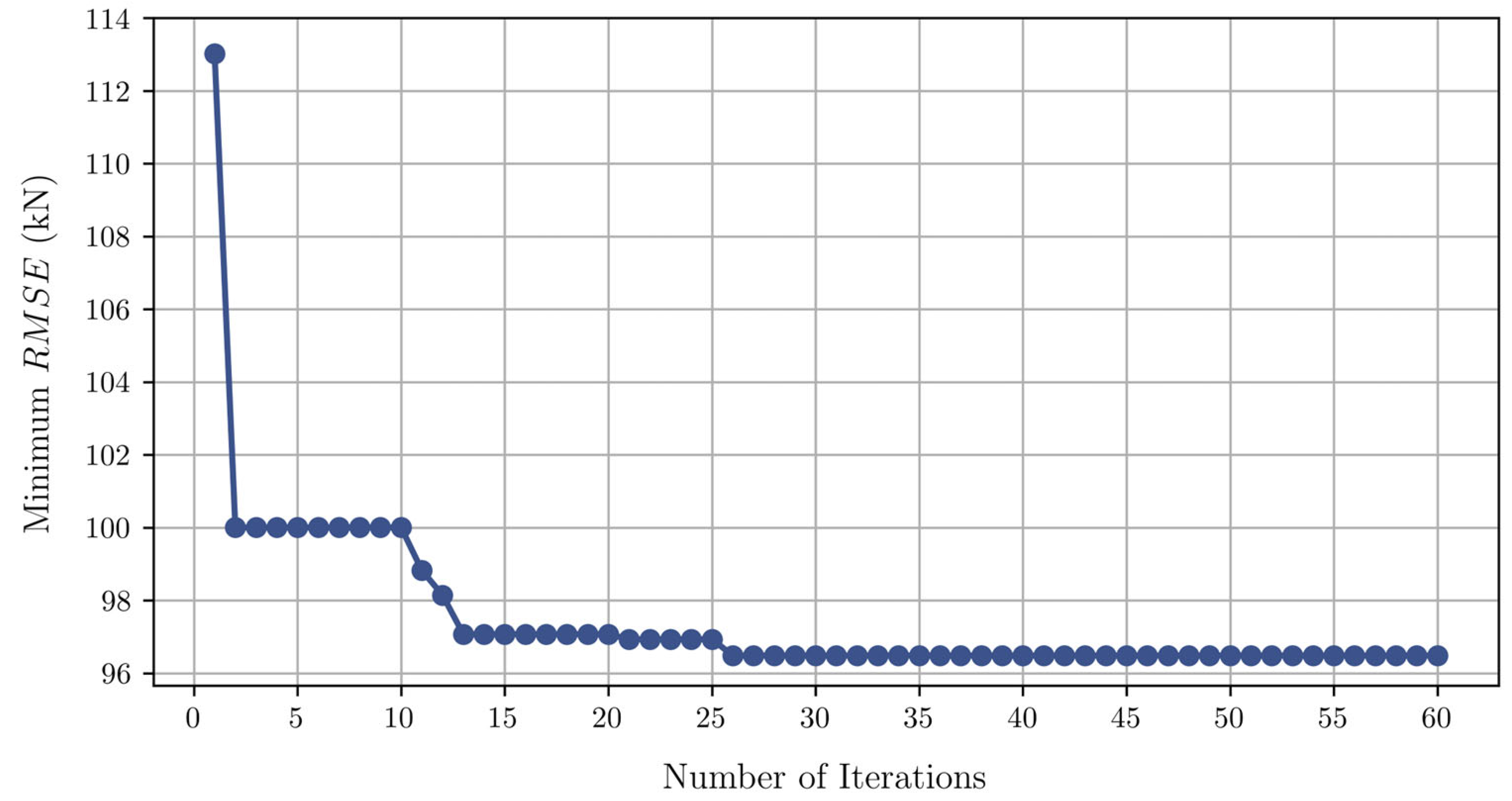
2.3. Hyperparameter Tuning

The hyperparameters of ML algorithms do not learn from the data. They are set by default and, in most cases, produce poor performance. Thus, the hyperparameters must be tuned to enhance predictive accuracy, accelerate convergence, mitigate overfitting, and improve robustness. In this research, the hyperparameters of selected ML algorithms were tuned using Bayesian optimization to find their optimal values. The optimization was performed using the GP minimize function as a probabilistic surrogate model combined with a 10-fold cross-validation (CV) method. The goal is to find the minimum RMSE scores of the validation dataset over 60 iterations. The search spaces and optimal values of the tuned hyperparameters for the selected models are provided in

Table 2. Hyperparameter spaces and values of optimized ML models.

Algorithm	Hyperparameter	Search Space	Optimal Value
RF	n_estimators	Integer (100, 1000)	783
	max_depth	Integer (10, 50)	14
	max_features	Integer (1, 16)	8
ET	n_estimators	Integer (100, 1000)	798
	max_depth	Integer (10, 50)	25
	max_features	Integer (1, 16)	15
AB	n_estimators	Integer (10, 60)	53
	learning_rate	Real (0.1, 1.0)	0.87037279320499
CB	iterations	Integer (100, 1300)	1300
	learning_rate	Real (0.01, 1.0)	0.06344784452431354
	depth	Integer (6, 7)	6
	l2_leaf_reg	Real (0.0, 1.0)	1.0

. Figure 6 illustrates the convergence curve plot for the optimized CB model.

2.4. Performance Metrics

After training and optimizing the predictive models, it is crucial to evaluate their performance using several quantitative key metrics, in addition to the robust 10-fold CV, to obtain a comprehensive understanding of the models’ predictive capabilities. In the current research, four statistical metrics in regression analysis including “coefficient of determination (R²)” (Equation (6)), “root mean square error (RMSE)” (Equation (7)), “mean absolute percentage error (MAPE)” (Equation (8)), and “mean absolute error (MAE)” (Equation (9)) were adopted to evaluate the CB and other developed ML models in predicting the SS of RCDBs [9]. The equations of these metrics are presented below.

$$R^2=1-{\displaystyle \frac{{\sum }_{i=1}^N{\left(P_i-T_i\right)}^2}{{\sum }_{i=1}^N{\left(P_i-\overline{T}\right)}^2}}$$

(6)

$$RMSE=\sqrt{{\displaystyle \frac{\sum _{i=1}^N{\left(P_i-T_i\right)}^2}{N}}}$$

(7)

$$MAPE={\displaystyle \frac{100\%}{N}}{\sum }_{i=1}^N\left|{\displaystyle \frac{P_i-T_i}{T_i}}\right|$$

(8)

$$MAE={\displaystyle \frac{\sum _{i=1}^N\left|P_i-T_i\right|}{N}}$$

(9)

where $P_i=$ predicted SS, $T_i=$ experimental SS, $\overline{T}=$ mean value of experimental SS, and $i=1,\dots ,N$ indicates the number of specimens in the database.

These metrics are commonly used in regression problems, particularly in structural engineering applications. The R² measures how well the overall established model fits the data and makes a prediction, based on the proportion of total variation of outputs. RMSE is the measure of the SD of prediction errors (residuals). It penalizes large errors more heavily than small errors and is sensitive to outliers. MAE measures error magnitude directly but is less sensitive to outliers than RMSE. Both RMSE and MAE express prediction errors in terms of units of the output variable. MAPE is a scale-independent metric that expresses prediction error as a percentage of the actual value. Statically, a higher value of R² and corresponding lower values of RMSE, MAE, and MAPE indicate the performance level of the model. However, the R² value is observed as the best metric for evaluation [93].

2.5. Interpretation of Predictive ML

After developing and evaluating the CB model for SS of RCDBs, it is essential to interpret the model prediction, as the general ML model is considered to some extent a “black box” model. Model interpretation provides an in-depth look at the decision-making behavior of a black box. It also increases the trust of users. In current research, the interpretation was achieved using the Shapley additive explanations (SHAP) algorithm and partial dependency plots.

2.5.1. SHAP Algorithm

SHAP is a game theory-based procedure for describing the performance of an ML model [94]. Recently, the SHAP has been widely employed as an efficient algorithm to explain the influence of each input feature on the ML model. This algorithm assigns a SHAP value to each input feature and quantifies their effects on the final predictions to produce an explainable ML model [95,96]. The explanation function $f\left(x\right)$ can be presented as follows:

$$f\left(X\right)={\varphi }_0+\sum _{i=1}^n{(\varphi }_i{X}_i^{\prime })$$

(10)

where ${\varphi }_0=$ predicted mean value of all specimens, $x^{\prime }=$ generalized value of input feature $\left(x\right)$, $n=$ total number of input features, and ${\varphi }_i=$ SHAP value.

$${\varphi }_i={\sum }_{S\subseteq F\backslash \left\{i\right\}} {\displaystyle \frac{\left|S\right|!(\left|F\right|-\left|S\right|-1)!}{\left|F\right|!}}\left[f_{SU\left\{i\right\}}\left(X_{SU\left\{i\right\}}\right)-f_S\left(X_S\right)\right]$$

(11)

where $F=$ a set input features, $S=$ a subset of $F$ where the parameters considering the index $i$ is suspended, and $X_S=$ a vector which contains the value of the input parameter in the subset $S$ [97].

2.5.2. Partial Dependency Plots (PDPs)

PDP indicates the functional relationship between a specific dataset of input variables and model output. It shows how predictions can be affected by the values of particular input variables [98]. Furthermore, the PDP reveals the influence of each variable on the outcomes of the developed predictive ML model. PDP is a global interpretation because it takes into consideration the entire database and provides the overall relationship between a feature and predicted values. PDPs are helpful visualizations of the contribution of every input feature toward the predicted output [98].

3. Results and Discussion

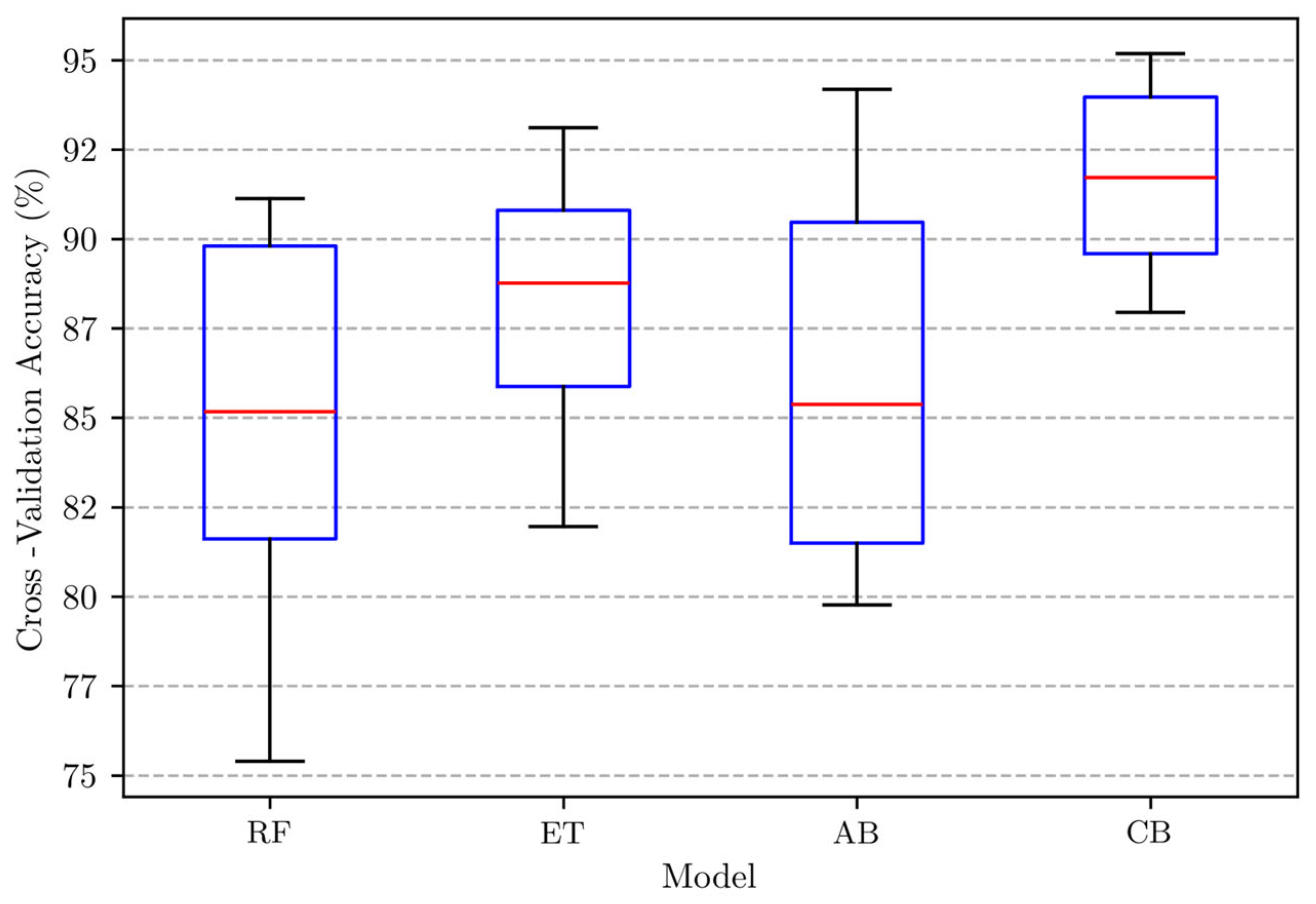
3.1. 10-Fold CV Performance Evaluation

During the optimization process, the performance of RF and AD models was slightly improved, but the ET model showed no improvement. This could be due to models’ complexity and capability, as well as the data characteristics under consideration. However, the performance of the CB model achieved a notable enhancement, as illustrated in Figure 6. The final results obtained from 10-fold CV on unseen data for the optimized models were visualized using boxplots, as shown in Figure 7. This visualization helps to understand not only the average performance but also the consistency and variability of performance across different folds of unseen data. In general, the size of boxes (the interquartile range) represents the variability in the scores. A smaller box indicates less variability, suggesting more consistent performance. A larger box indicates greater variability, suggesting instability or potential issues with performance. The red line in the middle of the boxes represents the median/mean value of scores, suggesting a high or poor performance. The whiskers at the ends of boxes represent the range of scores. A longer whisker suggests a wider range of performance, and vice versa. Accordingly, the CB model achieved the highest median value (91.7%), the smallest box, and shortest whiskers, exhibiting strong and consistent generalization performance over the other models. ET also achieved consistent performance (small box) but with a lower median value (88.8%) and a longer whisker. On the other hand, RF and AB showed unstable performance (large boxes, long whiskers, and low median/mean values). A more detailed evaluation can be found in the following subsection.

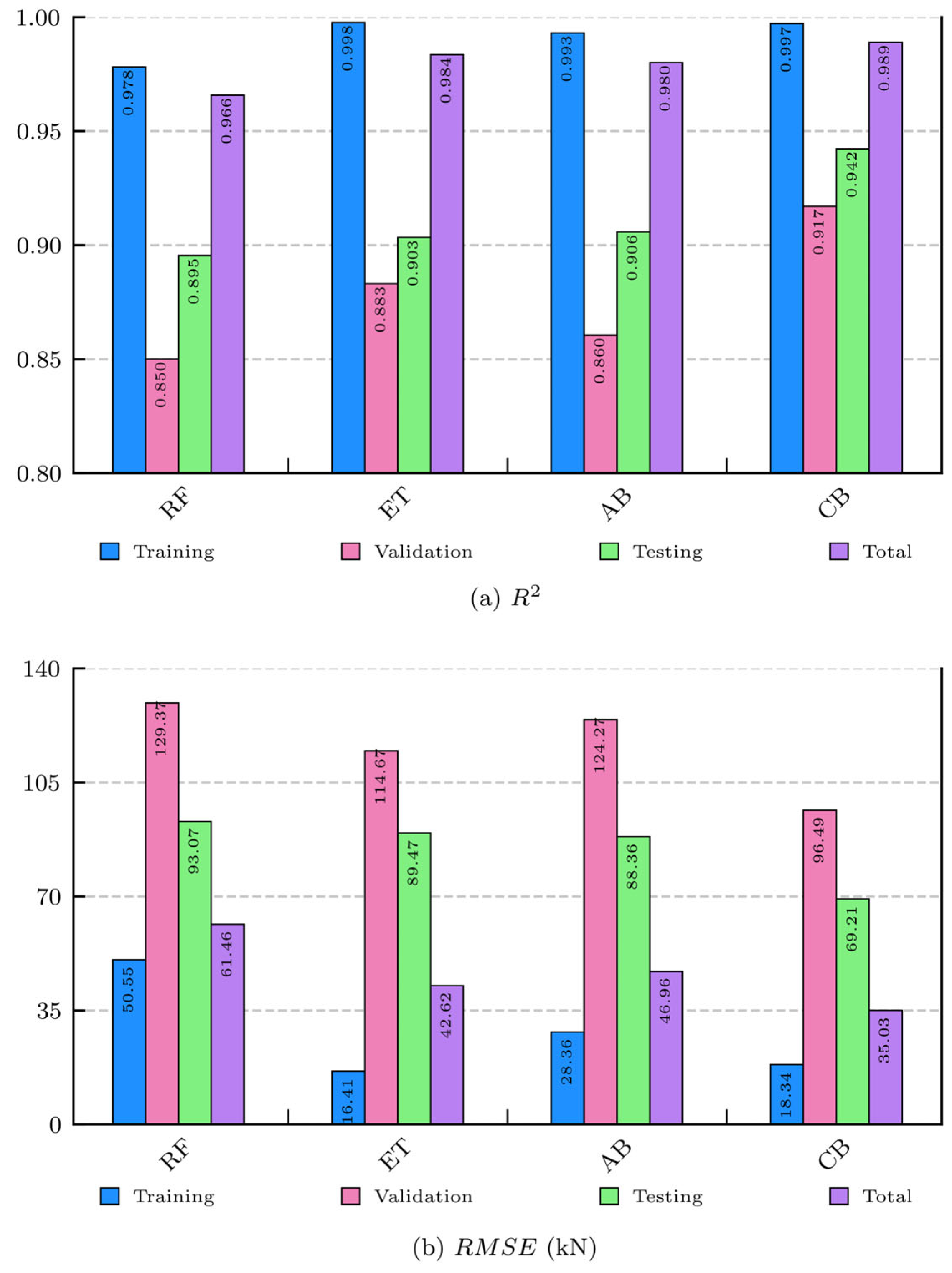
3.2. Overall Performance Evaluation

In this part, the performance of the CB model was evaluated and compared against those of the RF, ET, and AB models across various datasets based on the statistical metrics discussed in Section 2.4. Detailed information and rich visualization on the performance of optimized models are provided in

Table 3. Overall performance evaluation of optimized ML models.

Model	Dataset	Metric
		R2	RMSE (kN)	MAE (kN)	MAPE (%)
RF	Training	0.9782	50.5509	29.5371	8.1684
	Validation	0.8501	129.3699	76.1972	21.2943
	Testing	0.8955	93.0718	62.6384	19.0369
	Total	0.9658	61.4556	36.1573	10.3421
ET	Training	0.9977	16.4073	2.4859	0.7452
	Validation	0.8831	114.6653	66.3175	18.2174
	Testing	0.9034	89.4670	57.7167	16.8640
	Total	0.9836	42.6172	13.5320	3.9690
AB	Training	0.9931	28.3637	13.9013	9.0994
	Validation	0.8605	124.2699	78.8827	24.9258
	Testing	0.9058	88.3623	58.9152	20.5315
	Total	0.9800	46.9594	22.9041	11.3858
CB	Training	0.9971	18.3366	8.4077	2.9568
	Validation	0.9170	96.4863	56.8127	15.0108
	Testing	0.9422	69.2136	47.1074	14.4932
	Total	0.9889	35.0298	16.1476	5.2641

and Figure 8. Evidently, the CB model demonstrated the best overall performance, consistently obtained the highest R², and the lowest error metrics (RMSE, MAE, MAPE) across all datasets. Validation scores indicate that the mean value of R² is 0.9170, which is nearly equal to 1. The mean values of RMSE and MAE are 96.4863 kN and 56.8127 kN, respectively, which are considered relatively low compared to the mean value of the SS. Based on training/testing scores, the main values of R², RMSE, MAE, and MAPE are 0.9971/0.9422, 18.3366/69.2136 kN, 8.4077/47.1074 kN, and 2.9568/14.4932%, respectively. On the other hand, the RF, ET, and AB models obtained reasonable R² scores across all datasets. However, slightly high values of error scores were detected compared to the CB model. Thus, further investigation and evaluation are required to understand the nature of the errors for each model.

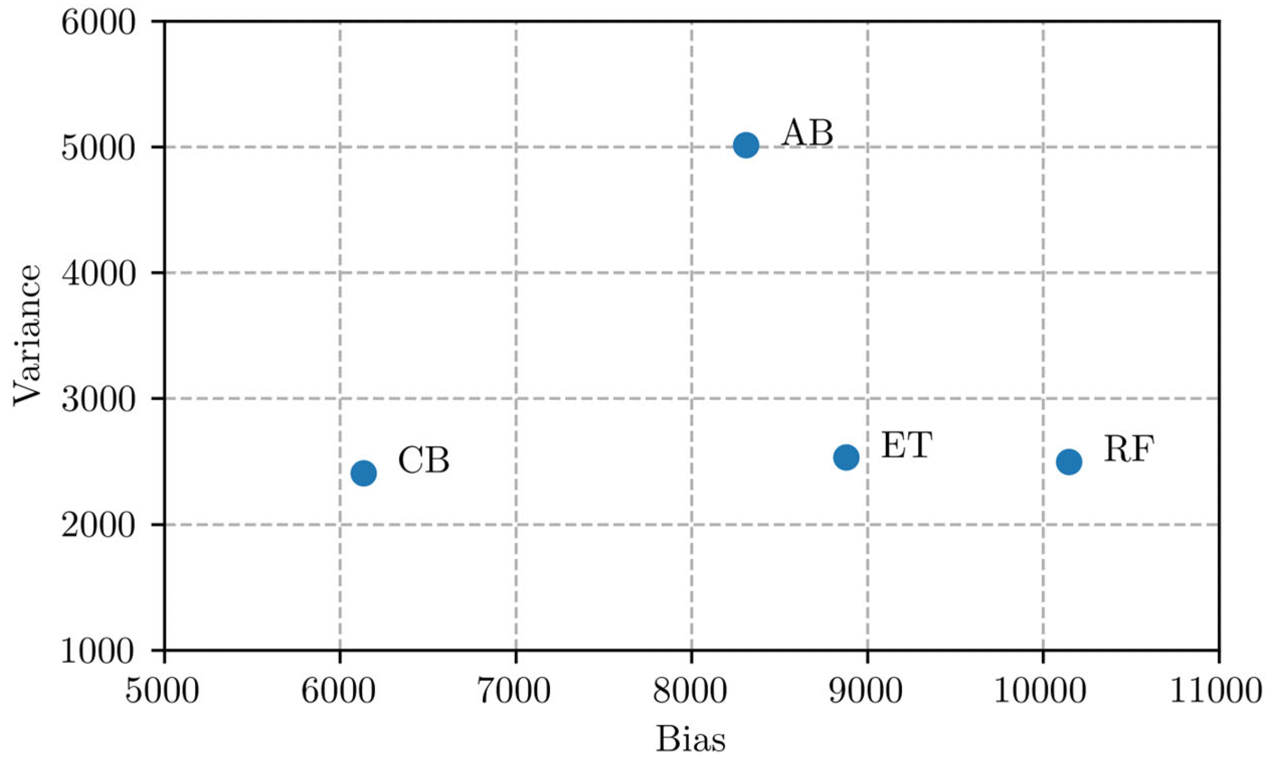
3.3. Bias-Variance Analysis

Bias and variance are two error sources causing overfitting/underfitting associated with ML algorithms. Hence, they must be extensively analyzed to identify the performance trend. In this study, the bias and variance scores of the optimized models were estimated using (bias_variance_decomp) function available on the mlxtend library, considering the mean squared error (MSE) as a loss function.

Table 4. Bias-variance evaluation for optimized ML models.

Model	Bias	Variance	MSE
RF	10,147.7445	2497.0147	12,644.7592
ET	8881.1901	2532.4058	11,413.5955
AB	8308.8276	5013.4415	13,322.2690
CB	6134.7950	2407.6251	8542.4200

provides the estimated bias, variance, and MSE scores for each model. Figure 9 also provides a rich visualization of the conducted bias-variance analysis.

The CB model exhibited the lowest bias and the lowest variance among all evaluated models. The low bias indicates that CB is very effective at accurately capturing the underlying patterns within the training dataset, leading to less systematic error in the prediction. The low variance suggests that its prediction is stable and not highly sensitive to the specific dataset used for training. This combination resulted in the lowest MSE score.

The ET model exhibited moderate bias and low variance. Its bias is higher than CB and AB but lower than RF. Its variance is very close to that of CB and RF but substantially lower than AB. This balance between bias and variance resulted in the second-lowest MSE score. ET offers a good compromise between capturing the true patterns and maintaining prediction stability, although its MSE score is high. Hence, it can still generalize well.

The RF model exhibited the highest bias and the second-lowest variance among the models. The high bias suggests it might not capture the underlying patterns as effectively as other models, potentially leading to underfitting. While its variance is not as high as AB, it resulted in a higher MSE score compared to CB and ET. This indicates that RF, in this context, is not achieving as optimal a bias-variance balance as the top two models.

The AB model exhibited a moderate bias, which is lower than RF and ET but higher than CB. However, it showed the highest variance by a considerable margin. This high variance suggests that AB predictions are more susceptible to fluctuations in the training dataset, potentially leading to overfitting. The high variance significantly resulted in its highest overall MSE score, indicating that AB struggles with the bias-variance trade-off, leaning towards higher variability in prediction.

Based on this analysis, CB appears to be the most effective model in minimizing the total prediction error and achieving a favorable bias-variance trade-off, hence providing the most consistent generalization performance, followed by the ET model. RF exhibited high bias with high total prediction error, indicating less flexibility in fitting the training dataset and potential for underfitting. AB, conversely, exhibited high variance with high total prediction error, indicating a greater sensitivity to noise and potential for overfitting. These findings align with the cross-validation results, where RF and AB showed an unstable performance in Figure 7 and a large discrepancy between training and validation scores in Table 3.

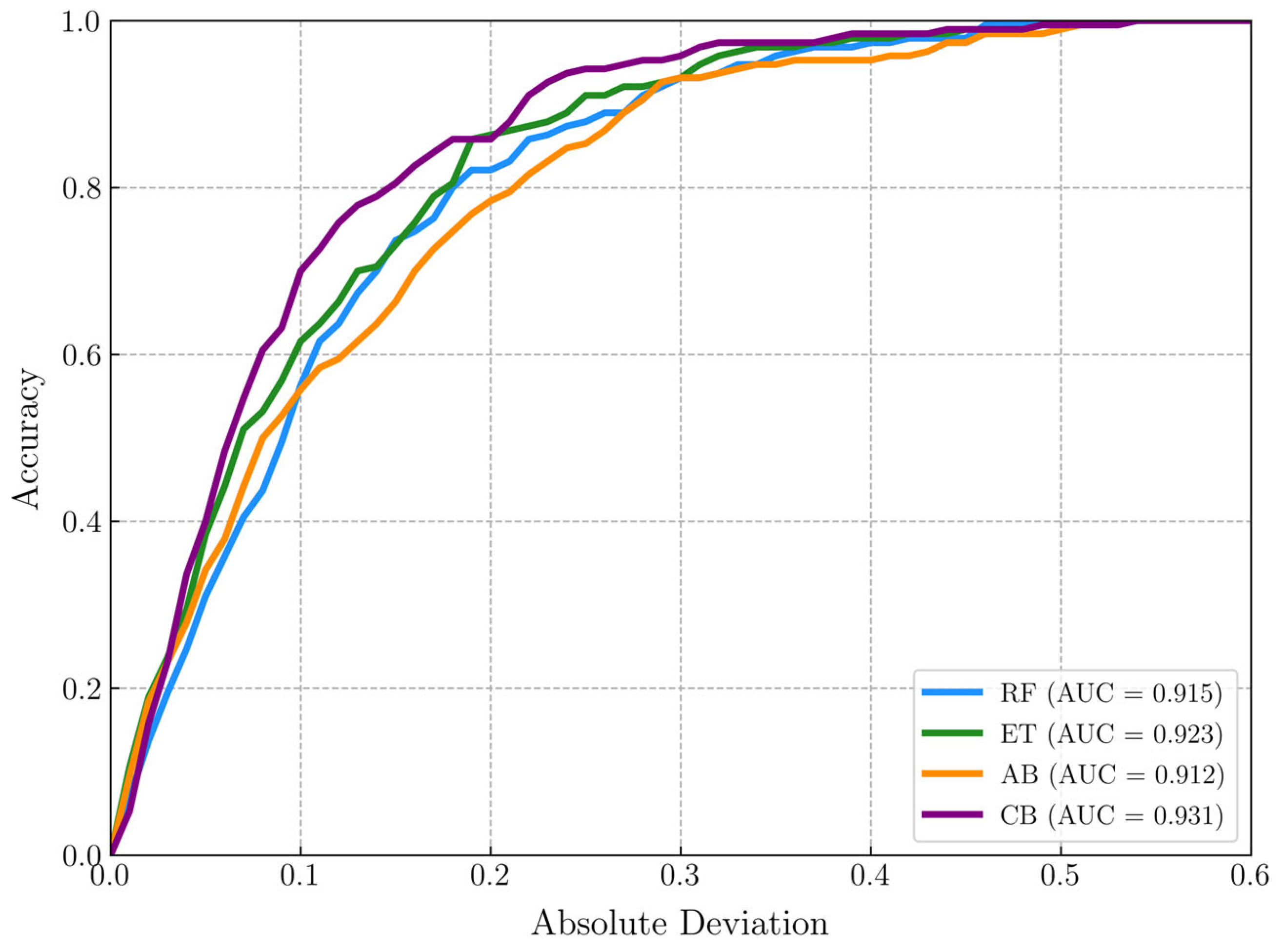
3.4. Prediction Accuracy of CB Model

The regression error characteristic (REC) curve is a visualizing tool used for evaluating the performance of regression models. The REC curve provides a comprehensive visualization of predictive accuracy by plotting the error tolerance (absolute deviation) on the x-axis against the model accuracy (fraction of predictions within that tolerance) on the y-axis. The area under the curve (AUC) provides a measure of overall performance. A larger AUC generally indicates better performance, as it means the model can achieve higher accuracy. The area over the curve (AOC) is considered a biased estimation of the expected error, which can be calculated as (AOC = 1 − AUC) [91]. Figure 10 illustrates the REC curves of the developed models in the testing phase. Obviously, the CB model secured the top performance rank by achieving the highest accuracy (AUC = 0.931) and the lowest error (AOC = 0.069). The CB model was also evaluated against ML models previously developed in the literature, as demonstrated in

Table 5. Comparison with previous ML models in predicting the SS of RCDBs.

Reference	Datapoints	Input Features	Best Model	R2
Feng et al. [9]	271	16	XGBoost	0.928
Truong et al. [10]	320	14	XGBoost	0.936
Ma et al. [11]	457	9	XGBoost	0.917
Nguyen et al. [12]	518	15	GPR	0.937
Tiwari et al. [13]	271	16	XGBoost	0.928
Abbas et al. [99]	386	22	RF	0.937
This study	950	16	CatBoost	0.942

. Again, the CB model developed in this research outperformed all existing models in predicting the SS of RCDBs by achieving the highest prediction accuracy.

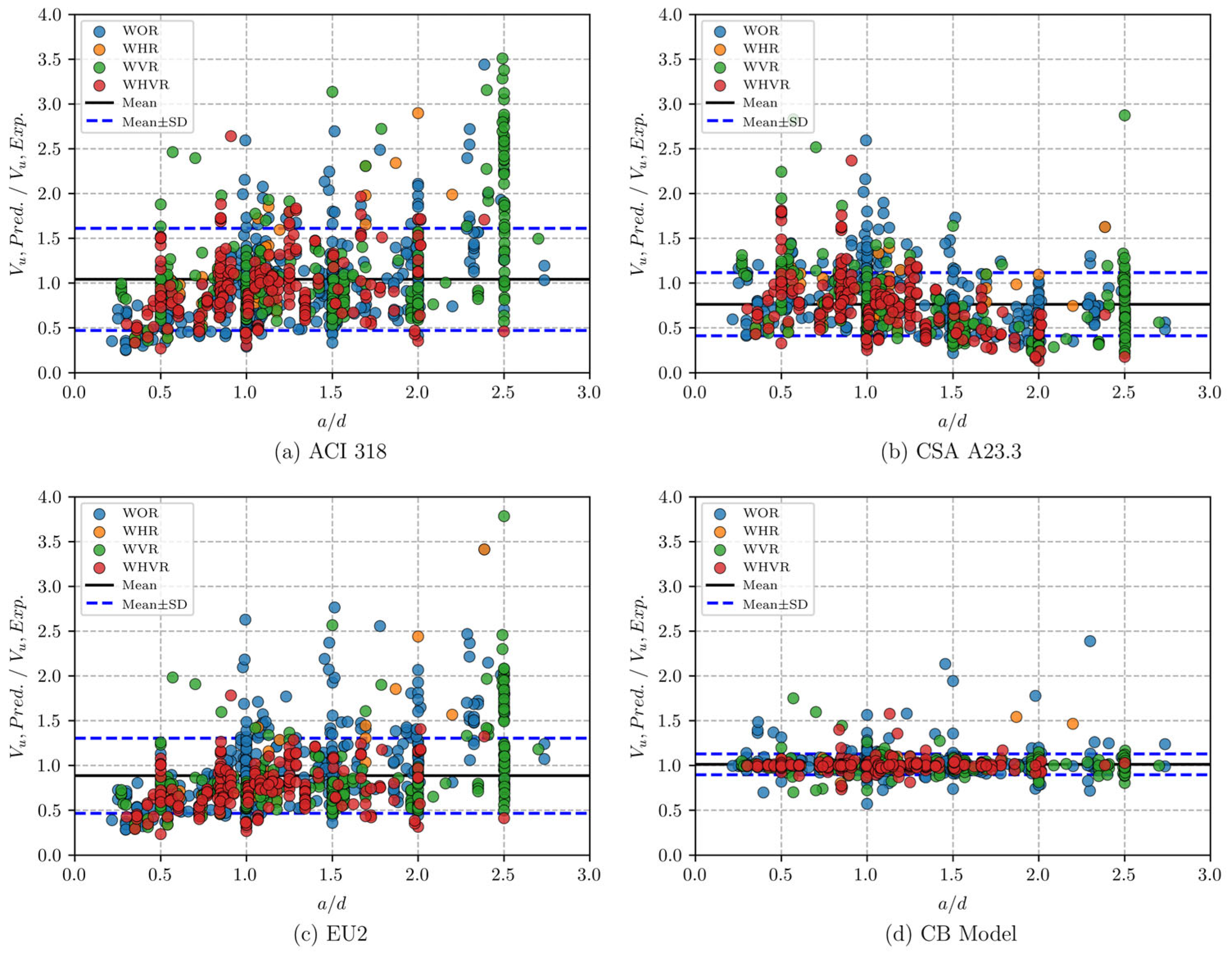
3.5. Comparison with Mechanics-Driven Models

The performance of the CB model was further evaluated against three traditional mechanics-driven models, which are outlined in Appendix A. Accordingly, the SS of RCDBs was predicted using the four models for the entire database. The scatter plot in Figure 11a–d illustrates the distribution of the predicted SS to experimental SS ratios (V_u, Pred./Vu, Exp.) with respect to a/d, where the different types of RCDBs (i.e., WOR, WHR, WVR, WHVR) are distinguished by different colors. More information on the predictive performances of the four models are revealed in

Table 6. Predictive performances of mechanics-driven and CB models.

Model	Vu, Pred./Vu, Exp.
	Min	Max	Mean	SD	COV (%)
ACI 318	0.252	7.606	1.042	0.570	54.717
CSA A23.3	0.133	2.873	0.763	0.353	46.176
EU2	0.234	3.784	0.886	0.419	47.339
CB	0.573	2.388	1.014	0.116	11.457

. It is observed that the performance of traditional models significantly varies. According to the mean values of (V_u, Pred./Vu, Exp.), CSA A23.3 and EU2 tended to underpredict the strength, while ACI 318 tended to overpredict the SS of RCDBs. In addition, the COV values of these three mechanics-driven models are considerably high compared to the CB model. As a comparison, the CB model even produced highly accurate predictions with a mean value of 1.014, an SD value of 0.116, and a COV value of only 11.457%.

Table 7. Predictive performances of mechanics-driven and CB models for different RCDB types.

Model	Vu, Pred./Vu, Exp.
	WOR			WHR			WVR			WHVR
	Mean	SD	COV (%)	Mean	SD	COV (%)	Mean	SD	COV (%)	Mean	SD	COV (%)
ACI 318	0.968	0.464	47.924	1.176	0.767	65.244	1.209	0.758	62.714	0.953	0.362	38.034
CSA A23.3	0.781	0.340	43.544	0.854	0.287	33.638	0.731	0.398	54.445	0.754	0.325	43.136
EU2	0.960	0.437	45.494	0.885	0.589	66.603	0.887	0.454	51.151	0.752	0.239	31.842
CB	1.024	0.145	14.135	1.023	0.120	11.688	1.005	0.094	9.369	1.004	0.071	7.090

also lists the predictive performances of the four models considering different types of RCDBs. As seen from Table 7, it is clear that the CB model performed reliably and accurately regardless of web reinforcement detail. It obtained mean values of (V_u, Pred./Vu, Exp.) between 1.004 and 1.024, SD values between 0.071 and 0.145, and COV values between 7.090% and 14.135%.

In short, this research proved that ML approaches have better performance and reliability than mechanics-driven approaches of standard codes. This is due to the fact that most traditional approaches are derived based on some assumptions or simplifications that fit particular applications. Furthermore, traditional approaches typically consider a safety factor in the formulation to mitigate the unknown uncertainties in design. Meanwhile, ML approaches do not require any assumptions or simplifications. The relationships between input and output features are detected by their inherent nature; hence, more complex behaviors are captured.

3.6. Interpretation of CB Model

The proposed CB model has a strong capability to predict the SS of RCDBs. Regardless, it is essential to interpret the model prediction in order to explore the impact of each input feature on the predicted output values. Therefore, the interpretation of the CB model was conducted herein, adopting the SHAP algorithm and PDPs analysis, which are discussed in Section 2.5.

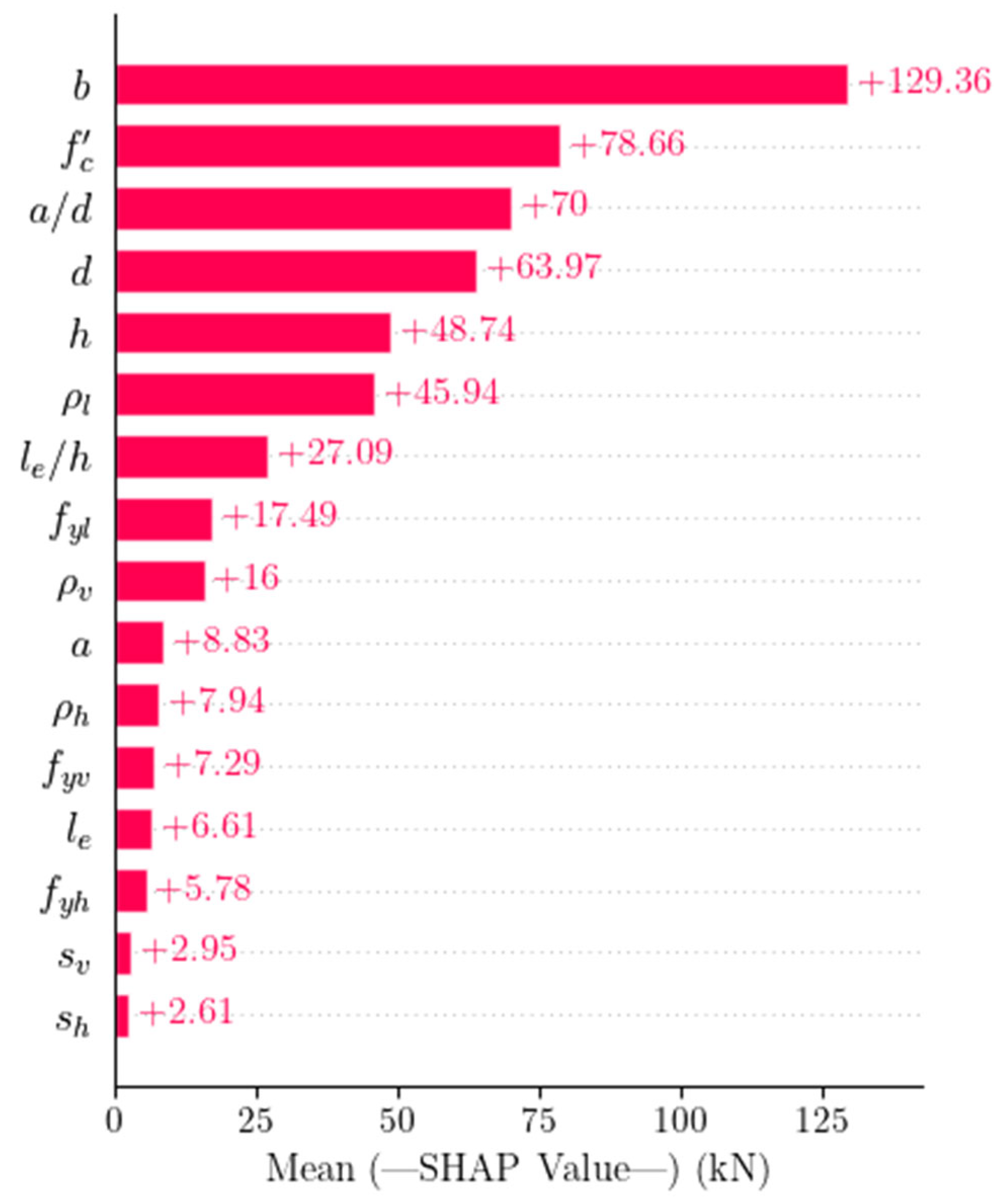
3.6.1. Feature Importance (FI)

In this part, the means of absolute SHAP values were used to measure the FI values for the entire database (globally) based on the CB model prediction. Figure 12 provides a rich visualization of the importance of input features. In the figure, the vertical axis represents the input features, which were sorted based on their importance in prediction, and the horizontal axis represents their corresponding importance values. If the FI value is far away from zero, it means the feature has a significant impact on the ML model prediction. Conversely, if the FI value is close to zero, it indicates the feature has less impact. The FI value has the same unit as the CB model output (kN).

Based on Figure 12, the most critical input features that significantly impacted the SS of RCDBs are $b$ and $f_c^{\prime }$. This observation aligns with mechanics-driven models outlined in Appendix A, which indicated that the SS of RCDBs strongly depends on $f_c^{\prime }$ and $b$. The second critical input features are the geometrical dimensions such as $a/d$, $d$, $h$ and $l_0/h$. This is logical given that these features are relevant to the SS mechanism, as RCDBs’ behavior (failure mode) is strongly dependent on cross-sectional properties. Surprisingly, the feature ${\rho }_l$ has a more significant impact on the SS than features ${\rho }_v$ and ${\rho }_h$. This is due to the fact that horizontal reinforcements mainly act as shear ties, which prevent buckling of vertical bars and improve the cohesion. Features $f_{yl}$ and ${\rho }_v$, which are related to the horizontal reinforcement and web reinforcement, respectively, have relatively similar impacts. Features $a$, and ${\rho }_h$ are considered less important. Other input features such as $f_{yv}$, $l_e$, $f_{yh}$, $s_v$, and $s_h$ are not that important since their FI values are small. However, deciding whether to exclude a specific feature from the model or not requires a comparative analysis with extensive optimization.

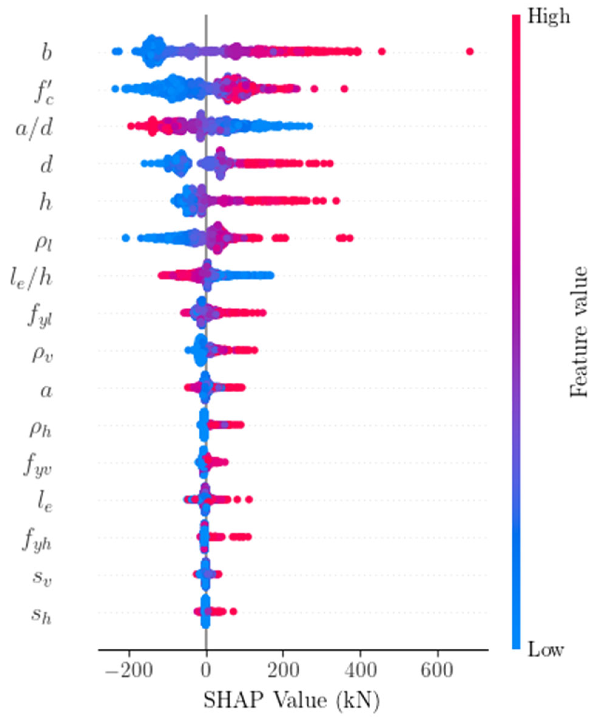
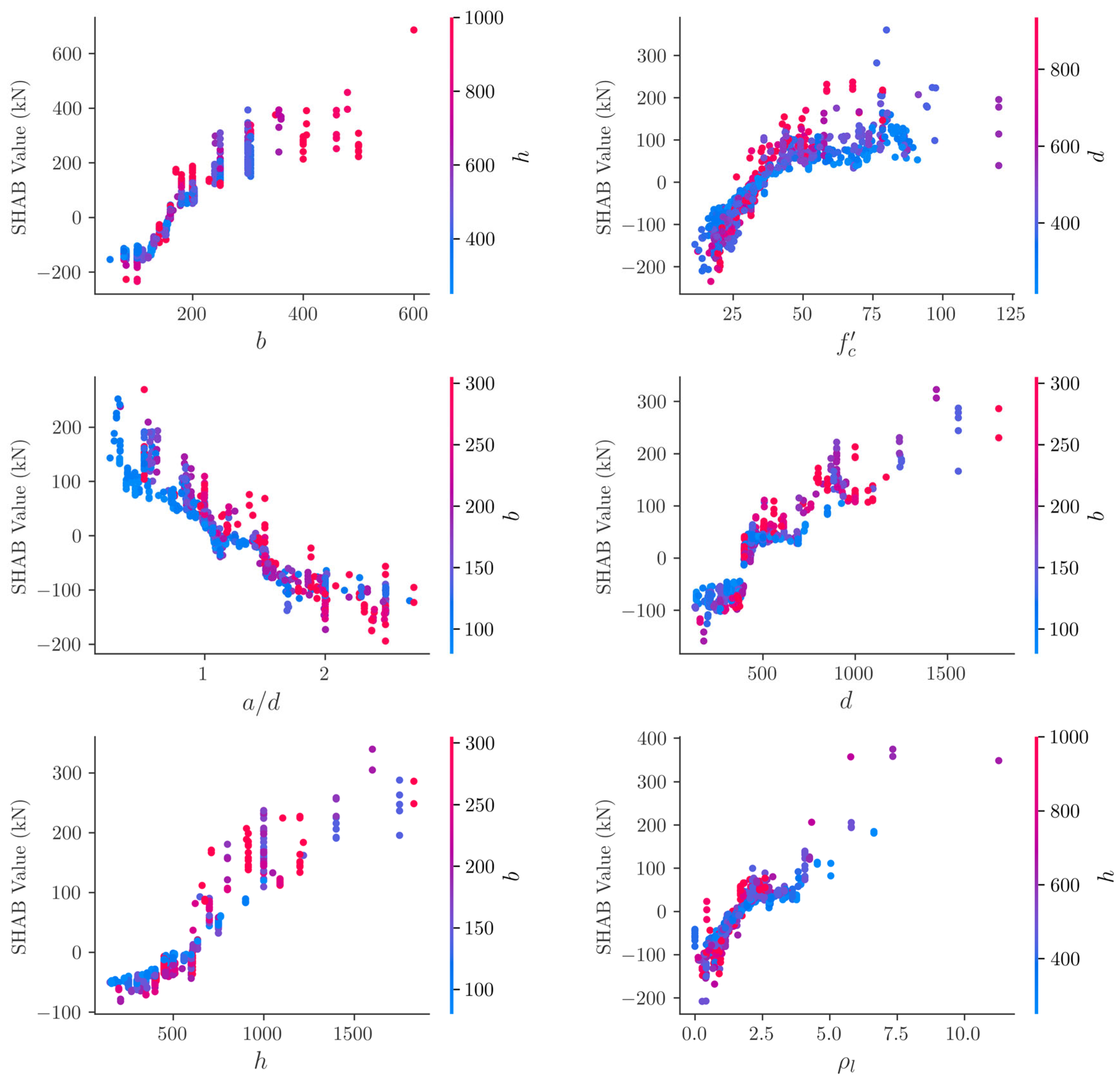
3.6.2. Global Interpretation

The SHAP algorithm can visualize the global interpretation of the predictive model. Hence, it is able to indicate how much each feature negatively or positively impacts the model output. In this part, the SHAP values were used to measure the input features’ impacts on model output for the entire database (globally) based on CB model prediction. Figure 13 provides a rich visualization of the global interpretation. The vertical axis represents the input features, which were sorted based on their importance in prediction, and the horizontal axis represents their corresponding SHAP values. The SHAP value of each input feature for a specific specimen was plotted as a dot on the graph, which could be negative or positive. A positive SHAP value denotes that the feature positively impacted the prediction, whereas a negative SHAP value denotes that the feature negatively impacted the prediction. The colors of the dots represent the impact values of input features on the prediction, ranging from blue (low) to red (high). By analyzing color distribution (blue indicating low value and red indicating high value), it is possible to identify whether low or high values tend to push the prediction in a negative or positive direction. SHAP value has the same unit as the CB model output (kN). Based on Figure 13, features $b$, $f_c^{\prime }$, $d$, $h$, and ${\rho }_l$ induced the highest positive impact on the predicted SS of RCDBs. On the other hand, features $a/d$ and $l_e/h$ negatively impacted the SS. This finding is consistent with mechanics-driven models outlined in Appendix A, which revealed that the SS of RCDBs is strongly dependent on $f_c^{\prime }$ and $b$.

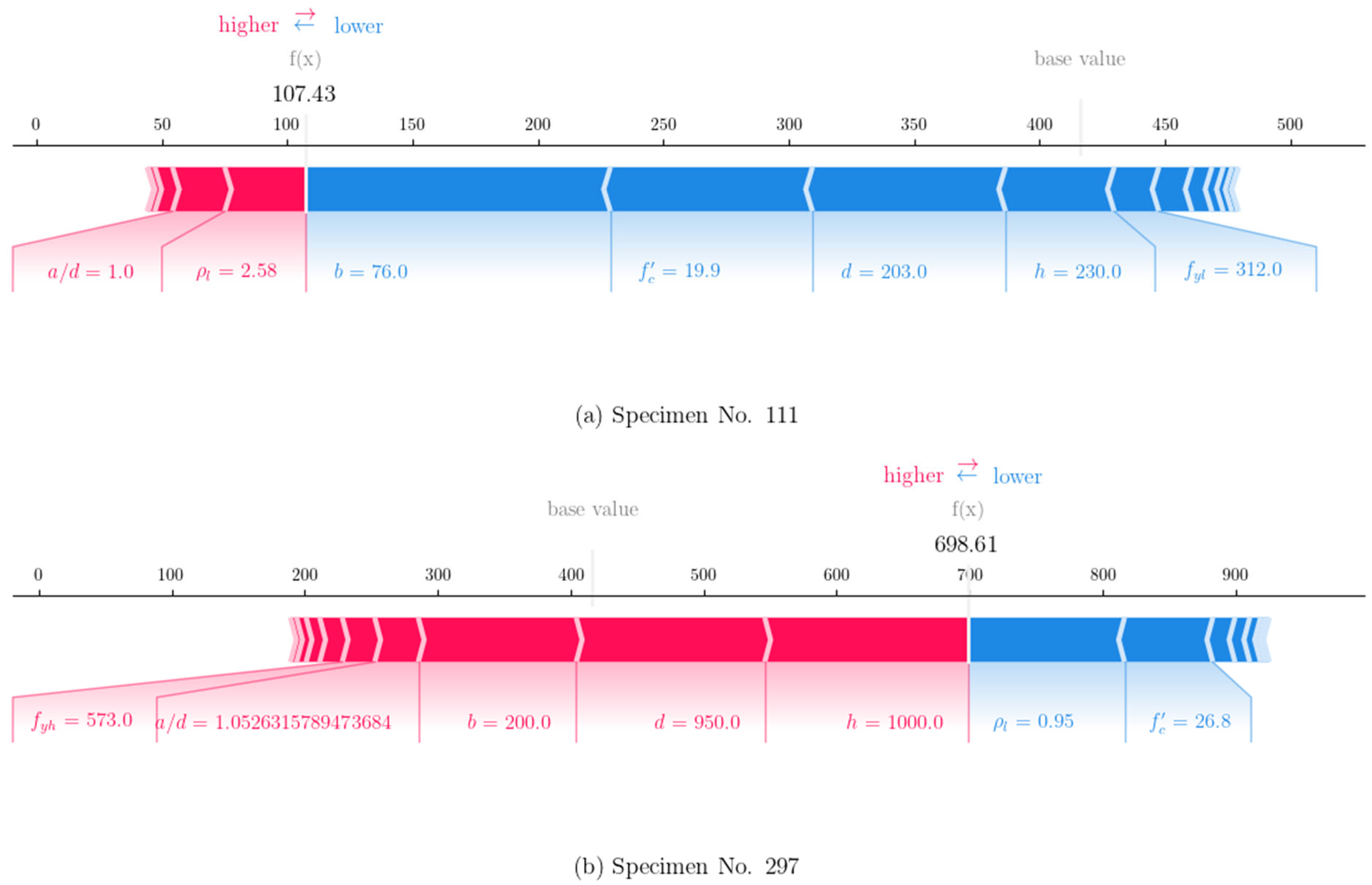
3.6.3. Local Interpretation

In addition to global, the SHAP algorithm can also visualize the local interpretation of the predictive model. It significantly enhances the prediction’s transparency, which traditional algorithms cannot achieve. In this part, the SHAP algorithm was used to measure the input features’ impacts on the output (locally) for two randomly selected specimens based on CB model prediction. Figure 14a,b provides the force plots of the local interpretation for the specimen (No. 111: G33S-31) tested by [52] and the specimen (No. 297: BM2/1.0 T1) tested by [57]. In these plots, the impact value of each input feature was expressed by length. The feature that positively impacted the prediction was assigned a red color, while the feature that negatively impacted the prediction was assigned a blue color. The mean value of the CB model output (416.10 kN) was identified as a base value for all specimens. For specimen No. 111, the CB model prediction was equal to 107.43 kN and its corresponding experimental value was 107.00 kN. The most significant input features that pushed down the base value were $b$, $f_c^{\prime }$, $d$, $h$, and $f_{yl}$, while features ${\rho }_l$ and $a/d$ tended to boost the base value. For specimen No. 297, the CB model prediction was equal to 698.61 kN and its corresponding experimental value was 700.00 kN. The most significant input features that boosted the base value were $h$, $d$, $b$, $a/d$, and $f_{yh}$, while features ${\rho }_l$ and $f_c^{\prime }$ tended to push down the base value. These findings are consistent with the global interpretation result, where the features $b$, $f_c^{\prime }$, $d$, $h$,, and ${\rho }_l$ have the largest contribution to the CB model prediction. In summary, the local interpretation offers engineers practical benefits when designing or retrofitting RCDBs. For designing, it reveals how these features impact the beam strength and potential failure mechanisms, allowing for an optimized design that achieves the desired SS within a few trials, hence saving time, labor, and materials. For retrofitting, it helps identify weak points in existing RCDBs by showing which features negatively impact the SS, enabling cost-effective strengthening strategies.

3.6.4. PDPs Analysis

Even though the SHAP plot in Section 3.6.2 successfully visualized the global impact of input features, the detailed relationships between input features and their SHAP values were not clarified. In this part, the PDP was adopted to clarify these relationships in detail based on CB model prediction. Figure 15 provides a rich visualization of the PDPs for the six critical input features over the entire database. PDPs can also explore the interaction between pairs of features. For each feature, its corresponding correlated feature is displayed on the right side of the plot by a colored bar. It is observed that SHAP values were increased almost linearly with increasing of $d$, $h$ and ${\rho }_l$, indicating a positive correlation between these features and the SS. In addition, features $b$ and $f_c^{\prime }$, exhibited nonlinear relationships with SHAP values. Increasing their values up to approximately 300 mm and 80 MPa, respectively, increased the SHAP values. Beyond these threshold values, the corresponding SHAP values were not increased. On the other hand, SHAP values were decreased linearly by increasing the features $a/d$, indicating a negative correlation between this feature and the SS. This observation is compatible with scientific knowledge and mechanics-driven models, which indicate that the SS of RCDBs mainly depends on geometric dimensions and concrete strength, followed by reinforcement properties.

4. Conclusions

This research established a newly comprehensive database of 950 experimental specimens of RCDBs failed in shear collected from open literature. Based on this database, an interpretable data-driven approach was developed using the CB algorithm for predicting the SS of RCDBs. The theoretical background and implementation procedure were given in detail. The performance of the enhanced CB model was then thoroughly evaluated and compared against three data-driven models developed in this research, as well as three prominent mechanics-driven models through several statistical indicators. Finally, the importance of input features and their impacts on CB model prediction were examined through interpretation from both global and local viewpoints, utilizing the SHAP algorithm with partial dependence plots to provide an in-depth look at the behavior of the black box. Consequently, the following findings are concluded:

• The CB model achieved the highest prediction accuracy (R²) and lowest errors (RMSE, MAE, and MAPE) compared to three other data-driven models, such as RF, ET, and AB.
• The CB model significantly outperformed the traditional mechanics-driven models such as ACI 318, CSA A23.3, and EU2 in terms of mean, SD, and COV.
• SHAP analysis revealed that CB models can efficiently capture the shear mechanism of RCDBs, which showed similar trends with mechanics-driven models. The geometric dimensions and concrete properties are the most influential input features on SS of RCDBs, followed by reinforcement properties.
• PDPs analysis indicated that SS of RCDBs can be significantly improved by increasing the values of $b$, $f_c^{\prime }$, and ${\rho }_l$ up to approximately 300 mm, 80 MPa, and 6%, respectively. In contrast, increasing the value of $a/d$ up to 2.5 can negatively influence the SS.

Accordingly, the proposed interpretable data-driven CB model has a high potential to be an alternative approach for design practice. This research is expected to be of interest to researchers and practitioners working at the intersection of structural engineering, data analytics, and intelligent systems. However, there is still room for further advancement and improvement, such as adding new data, using more intelligent feature selection and optimization techniques, as well as adopting new approaches to derive explicit mechanism-related equations. Thus, further investigations are encouraged in this direction for future research.

References

1. Ma, C.; Xie, C.; Tuohuti, A.; Duan, Y. Analysis of influencing factors on shear behavior of the reinforced concrete deep beams. J. Build. Eng. 2022, 45, 103383. [Google Scholar] [CrossRef]
2. Abbood, I.S. Strut-and-tie model and its applications in reinforced concrete deep beams: A comprehensive review. Case Stud. Constr. Mater. 2023, 19, e02643. [Google Scholar] [CrossRef]
3. Sanad, A.; Saka, M.P. Prediction of ultimate shear strength of reinforced-concrete deep beams using neural networks. J. Struct. Eng. 2001, 127, 818–828. [Google Scholar] [CrossRef]
4. Pal, M.; Deswal, S. Support vector regression based shear strength modelling of deep beams. Comput. Struct. 2011, 89, 1430–1439. [Google Scholar] [CrossRef]
5. Mohammadhassani, M.; Saleh, A.M.D.; Suhatril, M.; Safa, M. Fuzzy modelling approach for shear strength prediction of RC deep beams. Smart Struct. Syst. 2015, 16, 497–519. [Google Scholar] [CrossRef]
6. Chou, J.-S.; Ngo, N.-T.; Pham, A.-D. Shear strength prediction in reinforced concrete deep beams using nature-inspired metaheuristic support vector regression. J. Comput. Civ. Eng. 2016, 30, 04015002. [Google Scholar] [CrossRef]
7. Shahnewaz, M.; Rteil, A.; Alam, M.S. Shear strength of reinforced concrete deep beams—A review with improved model by genetic algorithm and reliability analysis. Structures 2020, 23, 494–508. [Google Scholar] [CrossRef]
8. Prayogo, D.; Cheng, M.-Y.; Wu, Y.-W.; Tran, D.-H. Combining machine learning models via adaptive ensemble weighting for prediction of shear capacity of reinforced-concrete deep beams. Eng. Comput. 2020, 36, 1135–1153. [Google Scholar] [CrossRef]
9. Feng, D.-C.; Wang, W.-J.; Mangalathu, S.; Hu, G.; Wu, T. Implementing ensemble learning methods to predict the shear strength of RC deep beams with/without web reinforcements. Eng. Struct. 2021, 235, 111979. [Google Scholar] [CrossRef]
10. Truong, G.T.; Choi, K.-K.; Nguyen, T.-H.; Kim, C.-S. Prediction of shear strength of RC deep beams using XGBoost regression with Bayesian optimization. Eur. J. Environ. Civ. Eng. 2023, 27, 4046–4066. [Google Scholar] [CrossRef]
11. Ma, C.; Wang, S.; Zhao, J.; Xiao, X.; Xie, C.; Feng, X. Prediction of shear strength of RC deep beams based on interpretable machine learning. Constr. Build. Mater. 2023, 387, 131640. [Google Scholar] [CrossRef]
12. Nguyen, K.L.; Trinh, H.T.; Nguyen, T.T.; Nguyen, H.D. Comparative study on the performance of different machine learning techniques to predict the shear strength of RC deep beams: Model selection and industry implications. Expert Syst. Appl. 2023, 230, 120649. [Google Scholar] [CrossRef]
13. Tiwari, A.; Gupta, A.K.; Gupta, T. A robust approach to shear strength prediction of reinforced concrete deep beams using ensemble learning with SHAP interpretability. Soft Comput. 2024, 28, 6343–6365. [Google Scholar] [CrossRef]
14. Adebar, P. One-way shear strength of large footings. Can. J. Civ. Eng. 2000, 27, 553–562. [Google Scholar] [CrossRef]
15. Aguilar, G.; Matamoros, A.B.; Parra-Montesinos, G.J.; Ramirez, J.A.; Wight, J.K. Experimental evaluation of design procedures for shear strength of deep reinforced concrete beams. ACI Struct. J. 2002, 99, 539–548. [Google Scholar] [CrossRef]
16. Ahmad, S.H.; Lue, D.M. Flexure-shear interaction of reinforced high strength concrete beams. ACI Struct. J. 1987, 84, 330–341. [Google Scholar] [CrossRef]
17. Ahmad, S.H.; Xie, Y.; Yu, T. Shear ductility of reinforced lightweight concrete beams of normal strength and high strength concrete. Cem. Concr. Compos. 1995, 17, 147–159. [Google Scholar] [CrossRef]
18. Akkaya, H.C.; Aydemir, C.; Arslan, G. Investigation on shear behavior of reinforced concrete deep beams without shear reinforcement strengthened with fiber reinforced polymers. Case Stud. Constr. Mater. 2022, 17, e01392. [Google Scholar] [CrossRef]
19. Albidah, A.S.; Alqarni, A.S.; Wasim, M.; Abadel, A.A. Influence of aggregate source and size on the shear behavior of high strength reinforced concrete deep beams. Case Stud. Constr. Mater. 2023, 19, e02260. [Google Scholar] [CrossRef]
20. Alcocer, S.M.; Uribe, C.M. Monolithic and cyclic behavior of deep beams designed using strut-and-tie models. ACI Struct. J. 2008, 105, 327–337. [Google Scholar] [CrossRef]
21. Arabzadeh, A.; Aghayari, R.; Rahai, A.R. Investigation of experimental and analytical shear strength of reinforced concrete deep beams. Int. J. Civ. Eng. 2011, 9, 207–214. [Google Scholar]
22. Brena, S.F.; Roy, N.C. Evaluation of load transfer and strut strength of deep beams with short longitudinal bar anchorages. ACI Struct. J. 2009, 106, 678–689. [Google Scholar] [CrossRef]
23. Clark, A.P. Diagonal tension in reinforced concrete beams. ACI J. Proc. 1951, 48, 145–156. [Google Scholar] [CrossRef]
24. Demir, A.; Caglar, N.; Ozturk, H. Parameters affecting diagonal cracking behavior of reinforced concrete deep beams. Eng. Struct. 2019, 184, 217–231. [Google Scholar] [CrossRef]
25. El-Sayed, A.K.; Shuraim, A.B. Size effect on shear resistance of high strength concrete deep beams. Mater. Struct. 2016, 49, 1871–1882. [Google Scholar] [CrossRef]
26. Garay, J.D.D.; Lubell, A.S. Behavior of concrete deep beams with high strength reinforcement. In Proceedings of the Structures Congress 2008: Crossing Borders, Vancouver, BC, Canada, 24–26 April 2008; pp. 1–10. [Google Scholar]
27. Garay-Moran, J.d.D.; Lubell, A.S. Behavior of deep beams containing high-strength longitudinal reinforcement. ACI Struct. J. 2016, 113, 17–28. [Google Scholar] [CrossRef]
28. Gerhard, T.S.; Manuel, R.F. Diagonal crack width control in short beams. ACI J. Proc. 1971, 68, 451–455. [Google Scholar] [CrossRef]
29. Gong, S. The shear strength capability of reinforced concrete deep beam under symmetric concentrated loads. J. Zhengzhou Technol. Inst. 1982, 1, 52–68. (In Chinese) [Google Scholar]
30. Hassan, T.K.; Seliem, H.M.; Dwairi, H.; Rizkalla, S.H.; Zia, P. Shear behavior of large concrete beams reinforced with high-strength steel. ACI Struct. J. 2008, 105, 173–179. [Google Scholar] [CrossRef]
31. Ismail, K.S.; Guadagnini, M.; Pilakoutas, K. Shear behavior of reinforced concrete deep beams. ACI Struct. J. 2017, 114, 87–99. [Google Scholar] [CrossRef]
32. Kani, G.N.J. How safe are our large reinforced concrete beams? ACI J. Proc. 1967, 64, 128–141. [Google Scholar] [CrossRef]
33. Kondalraj, R.; Rao, G.A. Experimental verification of ACI 318 strut-and-tie method for design of deep beams without web reinforcement. ACI Struct. J. 2021, 118, 139–152. [Google Scholar] [CrossRef]
34. Kong, F.-K.; Robins, P.J.; Cole, D.F. Web reinforcement effects on deep beams. ACI J. Proc. 1970, 67, 1010–1018. [Google Scholar] [CrossRef]
35. Kong, P.Y.L.; Rangan, B.V. Shear strength of high-performance concrete beams. ACI Struct. J. 1998, 95, 677–688. [Google Scholar] [CrossRef]
36. Lee, D. An experimental investigation in the effects of detailing on the shear behaviour of deep beams. Master’s Thesis, University of Toronto, Toronto, ON, Canada, 1982. [Google Scholar]
37. Leonhardt, F.; Walther, R. The stuttgart shear tests. 318Reference 1962, 11, 134. [Google Scholar]
38. Li, Y.; Chen, H.; Yi, W.-J.; Peng, F.; Li, Z.; Zhou, Y. Effect of member depth and concrete strength on shear strength of RC deep beams without transverse reinforcement. Eng. Struct. 2021, 241, 112427. [Google Scholar] [CrossRef]
39. Liu, L.; Xie, L.; Chen, M. The shear strength capability of reinforced concrete deep flexural member. Build. Struct. 2000, 30, 19–22. (In Chinese) [Google Scholar]
40. Londhe, R.S. Shear strength analysis and prediction of reinforced concrete transfer beams in high-rise buildings. Struct. Eng. Mech. 2011, 37, 39–59. [Google Scholar] [CrossRef]
41. Lu, W.-Y.; Chu, C.-H. Tests of high-strength concrete deep beams. Mag. Concr. Res. 2019, 71, 184–194. [Google Scholar] [CrossRef]
42. Lu, W.-Y.; Lin, I.-J.; Yu, H.-W. Shear strength of reinforced concrete deep beams. ACI Struct. J. 2013, 110, 671–680. [Google Scholar] [CrossRef]
43. Manuel, R.F. Failure of deep beams. ACI Symp. Publ. 1974, 42, 425–440. [Google Scholar] [CrossRef]
44. Manuel, R.F.; Slight, B.W.; Suter, G.T. Deep beam behavior affected by length and shear span variations. ACI J. Proc. 1971, 68, 954–958. [Google Scholar] [CrossRef]
45. Mathey, R.G.; Watstein, D. Shear strength of beams without web reinforcement containing deformed bars of different yield strengths. ACI J. Proc. 1963, 60, 183–208. [Google Scholar] [CrossRef]
46. Mihaylov, B.I.; Bentz, E.C.; Collins, M.P. Behavior of large deep beams subjected to monotonic and reversed cyclic shear. ACI Struct. J. 2010, 107, 726–734. [Google Scholar] [CrossRef]
47. Mohammadhassani, M.; Jumaat, M.Z.; Jameel, M.; Badiee, H.; Arumugam, A.M.S. Ductility and performance assessment of high strength self compacting concrete (HSSCC) deep beams: An experimental investigation. Nucl. Eng. Des. 2012, 250, 116–124. [Google Scholar] [CrossRef]
48. Moody, K.G.; Viest, I.M.; Elstner, R.C.; Hognestad, E. Shear strength of reinforced concrete beams part 1-tests of simple beams. ACI J. Proc. 1954, 51, 317–332. [Google Scholar] [CrossRef]
49. Morrow, J.; Viest, I.M. Shear strength of reinforced concrete frame members without web reinforcement. ACI J. Proc. 1957, 53, 833–869. [Google Scholar] [CrossRef]
50. Mphonde, A.G.; Frantz, G.C. Shear tests of high- and low-strength concrete beams without stirrups. ACI J. Proc. 1984, 81, 350–357. [Google Scholar] [CrossRef]
51. Oh, J.-K.; Shin, S.-W. Shear strength of reinforced high-strength concrete deep beams. ACI Struct. J. 2001, 98, 164–173. [Google Scholar] [CrossRef]
52. Paiva, H.A.R.d.; Siess, C.P. Strength and behavior of deep beams in shear. J. Struct. Div. 1965, 91, 19–41. [Google Scholar] [CrossRef]
53. Pendyala, R.S.; Mendis, P. Experimental study on shear strength of high-strength concrete beams. ACI Struct. J. 2000, 97, 564–571. [Google Scholar] [CrossRef]
54. Proestos, G.T.; Bentz, E.C.; Collins, M.P. Maximum shear capacity of reinforced concrete members. ACI Struct. J. 2018, 115, 1463–1473. [Google Scholar] [CrossRef]
55. Quintero-Febres, C.G.; Parra-Montesinos, G.; Wight, J.K. Strength of struts in deep concrete members designed using strut-and-tie method. ACI Struct. J. 2006, 103, 577–586. [Google Scholar] [CrossRef]
56. Ramakrishnan, V.; Ananthanarayana, Y. Ultimate strength of deep beams in shear. ACI J. Proc. 1968, 65, 87–98. [Google Scholar] [CrossRef]
57. Rogowsky, D.M.; MacGregor, J.G.; Ong, S.Y. Tests of reinforced concrete deep beams. ACI J. Proc. 1986, 83, 614–623. [Google Scholar] [CrossRef]
58. Roller, J.J.; Russel, H.G. Shear strength of high-strength concrete beams with web reinforcement. ACI Struct. J. 1990, 87, 191–198. [Google Scholar] [CrossRef]
59. Sagaseta, J.; Vollum, R.L. Shear design of short-span beams. Mag. Concr. Res. 2010, 62, 267–282. [Google Scholar] [CrossRef]
60. Sahoo, D.K.; Sagi, M.S.V.; Singh, B.; Bhargava, P. Effect of detailing of web reinforcement on the behavior of bottle-shaped struts. J. Adv. Concr. Technol. 2010, 8, 303–314. [Google Scholar] [CrossRef]
61. Salamy, M.R.; Kobayashi, H.; Unjoh, S. Experimental and analytical study on RC deep beams. Asian J. Civ. Eng. (Build. Hous.) 2005, 6, 409–421. [Google Scholar]
62. Sarsam, K.F.; Al-Musawi, J.M.S. Shear design of high- and normal strength concrete beams with web reinforcement. ACI Struct. J. 1992, 89, 658–664. [Google Scholar] [CrossRef]
63. Senturk, A.E.; Higgins, C. Evaluation of reinforced concrete deck girder bridge bent caps with 1950s vintage details: Analytical methods. ACI Struct. J. 2010, 107, 544–553. [Google Scholar] [CrossRef]
64. Shin, S.-W.; Lee, K.-S.; Moon, J.-I.; Ghosh, S.K. Shear strength of reinforced high-strength concrete beams with shear span-to-depth ratios between 1.5 and 2.5. ACI Struct. J. 1999, 96, 549–556. [Google Scholar] [CrossRef]
65. Shuraim, A.B.; El-Sayed, A.K. Experimental verification of strut and tie model for HSC deep beams without shear reinforcement. Eng. Struct. 2016, 117, 71–85. [Google Scholar] [CrossRef]
66. Smith, K.N.; Vantsiotis, A.S. Shear strength of deep beams. ACI J. Proc. 1982, 79, 201–213. [Google Scholar] [CrossRef]
67. Subedi, N.K.; Vardy, A.E.; Kubotat, N. Reinforced concrete deep beams some test results. Mag. Concr. Res. 1986, 38, 206–219. [Google Scholar] [CrossRef]
68. Tan, K.H.; Cheng, G.H.; Cheong, H.K. Size effect in shear strength of large beams—Behaviour and finite element modelling. Mag. Concr. Res. 2005, 57, 497–509. [Google Scholar] [CrossRef]
69. Tan, K.H.; Lu, H.Y. Shear behavior of large reinforced concrete deep beams and code comparisons. ACI Struct. J. 1999, 96, 836–846. [Google Scholar] [CrossRef]
70. Tan, K.-H.; Cheng, G.-H.; Zhang, N. Experiment to mitigate size effect on deep beams. Mag. Concr. Res. 2008, 60, 709–723. [Google Scholar] [CrossRef]
71. Tan, K.-H.; Kong, F.-K.; Teng, S.; Guan, L. High-strength concrete deep beams with effective span and shear span variations. ACI Struct. J. 1995, 92, 395–405. [Google Scholar] [CrossRef]
72. Tan, K.-H.; Kong, F.-K.; Teng, S.; Weng, L.-W. Effect of web reinforcement on high-strength concrete deep beams. ACI Struct. J. 1997, 94, 572–582. [Google Scholar] [CrossRef]
73. Tan, K.-H.; Teng, S.; Kong, F.-K.; Lu, H.-Y. Main tension steel in high strength concrete deep and short beams. ACI Struct. J. 1997, 94, 752–768. [Google Scholar] [CrossRef]
74. Tanimura, Y.; Sato, T. Evaluation of shear strength of deep beams with stirrups. Q. Rep. RTRI 2005, 46, 53–58. [Google Scholar] [CrossRef]
75. Tuchscherer, R.; Kettelkamp, J. Estimating the service-level cracking behavior of deep beams. ACI Struct. J. 2018, 115, 875–883. [Google Scholar] [CrossRef]
76. Walravena, J.; Lehwalter, N. Size effects in short beams loaded in shear. ACI Struct. J. 1994, 91, 585–593. [Google Scholar] [CrossRef]
77. Watstein, D.; Mathey, R.G. Strains in beams having diagonal cracks. ACI J. Proc. 1958, 55, 717–728. [Google Scholar] [CrossRef]
78. Wei, H.; Wu, T.; Sun, L.; Liu, X. Evaluation of cracking and serviceability performance of lightweight aggregate concrete deep beams. KSCE J. Civ. Eng. 2020, 24, 3342–3355. [Google Scholar] [CrossRef]
79. Yang, K.-H.; Chung, H.-S.; Lee, E.-T.; Eun, H.-C. Shear characteristics of high-strength concrete deep beams without shear reinforcements. Eng. Struct. 2003, 25, 1343–1352. [Google Scholar] [CrossRef]
80. Zhang, J.-H.; Li, S.-S.; Xie, W.; Guo, Y.-D. Experimental study on shear capacity of high strength reinforcement concrete deep beams with small shear span–depth ratio. Materials 2020, 13, 1218. [Google Scholar] [CrossRef]
81. Zhang, N.; Tan, K.-H. Size effect in RC deep beams: Experimental investigation and STM verification. Eng. Struct. 2007, 29, 3241–3254. [Google Scholar] [CrossRef]
82. Zhang, N.; Tan, K.-H.; Leong, C.-L. Single-span deep beams subjected to unsymmetrical loads. J. Struct. Eng. 2009, 135, 239–252. [Google Scholar] [CrossRef]
83. Xu, J.-G.; Chen, S.-Z.; Xu, W.-J.; Shen, Z.-S. Concrete-to-concrete interface shear strength prediction based on explainable extreme gradient boosting approach. Constr. Build. Mater. 2021, 308, 125088. [Google Scholar] [CrossRef]
84. Ye, M.; Li, L.; Yoo, D.-Y.; Li, H.; Zhou, C.; Shao, X. Prediction of shear strength in UHPC beams using machine learning-based models and SHAP interpretation. Constr. Build. Mater. 2023, 408, 133752. [Google Scholar] [CrossRef]
85. Rahman, J.; Ahmed, K.S.; Khan, N.I.; Islam, K.; Mangalathu, S. Data-driven shear strength prediction of steel fiber reinforced concrete beams using machine learning approach. Eng. Struct. 2021, 233, 111743. [Google Scholar] [CrossRef]
86. Thai, H.-T. Machine learning for structural engineering: A state-of-the-art review. Structures 2022, 38, 448–491. [Google Scholar] [CrossRef]
87. Geurts, P.; Ernst, D.; Wehenkel, L. Extremely randomized trees. Machine Learning 2006, 63, 3–42. [Google Scholar] [CrossRef]
88. Dahesh, A.; Tavakkoli-Moghaddam, R.; Wassan, N.; Tajally, A.; Daneshi, Z.; Erfani-Jazi, A. A hybrid machine learning model based on ensemble methods for devices fault prediction in the wood industry. Expert Syst. Appl. 2024, 249, 123820. [Google Scholar] [CrossRef]
89. Wakjira, T.G.; Al-Hamrani, A.; Ebead, U.; Alnahhal, W. Shear capacity prediction of FRP-RC beams using single and ensenble ExPlainable Machine learning models. Compos. Struct. 2022, 287, 115381. [Google Scholar] [CrossRef]
90. Prokhorenkova, L.; Gusev, G.; Vorobev, A.; Dorogush, A.V.; Gulin, A. CatBoost: Unbiased boosting with categorical features. In Proceedings of the 32nd International Conference on Neural Information Processing Systems, Montréal, QC, Canada, 3–8 December 2018; pp. 6639–6649. [Google Scholar]
91. Pal, A.; Ahmed, K.S.; Mangalathu, S. Data-driven machine learning approaches for predicting slump of fiber-reinforced concrete containing waste rubber and recycled aggregate. Constr. Build. Mater. 2024, 417, 135369. [Google Scholar] [CrossRef]
92. Alsulamy, S. Predicting construction delay risks in Saudi Arabian projects: A comparative analysis of CatBoost, XGBoost, and LGBM. Expert Syst. Appl. 2025, 268, 126268. [Google Scholar] [CrossRef]
93. de-Prado-Gil, J.; Palencia, C.; Silva-Monteiro, N.; Martínez-García, R. To predict the compressive strength of self compacting concrete with recycled aggregates utilizing ensemble machine learning models. Case Stud. Constr. Mater. 2022, 16, e01046. [Google Scholar] [CrossRef]
94. Lundberg, S.M.; Lee, S.-I. A unified approach to interpreting model predictions. In Proceedings of the 31st International Conference on Neural Information Processing Systems, Long Beach, CA, USA, 4–9 December 2017; pp. 4768–4777. [Google Scholar]
95. Liu, T.; Cakiroglu, C.; Islam, K.; Wang, Z.; Nehdi, M.L. Explainable machine learning model for predicting punching shear strength of FRC flat slabs. Eng. Struct. 2024, 301, 117276. [Google Scholar] [CrossRef]
96. Zhang, S.-Y.; Chen, S.-Z.; Jiang, X.; Han, W.-S. Data-driven prediction of FRP strengthened reinforced concrete beam capacity based on interpretable ensemble learning algorithms. Structures 2022, 43, 860–877. [Google Scholar] [CrossRef]
97. Kashem, A.; Karim, R.; Malo, S.C.; Das, P.; Datta, S.D.; Alharthai, M. Hybrid data-driven approaches to predicting the compressive strength of ultra-high-performance concrete using SHAP and PDP analyses. Case Stud. Constr. Mater. 2024, 20, e02991. [Google Scholar] [CrossRef]
98. Zhang, J.; Li, D.; Wang, Y. Toward intelligent construction: Prediction of mechanical properties of manufactured-sand concrete using tree-based models. J. Clean. Prod. 2020, 258, 120665. [Google Scholar] [CrossRef]
99. Abbas, Y.M.; Albidah, A.S. Enhanced data-driven shear strength prediction for RC deep beams: Analyzing key influencing factors and model performance. Structures 2024, 70, 107651. [Google Scholar] [CrossRef]
100. ACI 318-19; Building Code Requirements for Structural Concrete and Commentary. American Concrete Institute (ACI): Farmington Hills, MI, USA, 2019; p. 624.
101. CSA A23.3:19; Design of Concrete Structures, 17th ed. Canadian Standards Association: Toronto, ON, Canada, 2019; p. 301.
102. EN 1992-1-1; Eurocode 2 Design of Concrete Structures–Part 1-1: General Rules and Rules for Buildings. British Standard Institution (BSI): London, UK, 2015; p. 230.
Figure 1. Failure mechanisms in RCDBs.
Asi 08 00096 g001
Figure 2. Types of RCDBs based on web reinforcement.
Asi 08 00096 g002
Figure 3. Statistical distributions for all features included in the database. The inputs are indicated by a blue color, while the output is indicated by a green color.
Asi 08 00096 g003
Figure 4. Graphical illustration of RF [86].
Asi 08 00096 g004
Figure 5. Graphical illustration of AB [86].
Asi 08 00096 g005
Figure 6. Convergence curve of optimized CB model.
Asi 08 00096 g006
Figure 7. CV performance for optimized ML models.
Asi 08 00096 g007
Figure 8. Bar plots of evaluation indices for optimized ML models. (a) R2 score. (b) RMSE score.
Asi 08 00096 g008
Figure 9. Plot of bias-variance analysis for optimized ML models.
Asi 08 00096 g009
Figure 10. REC curves for optimized ML models.
Asi 08 00096 g010
Figure 11. Predicted SS by mechanics-driven and CB models for different RCDB types. (a) ACI 318. (b) CSA A23.3. (c) EU2. (d) CB model.
Asi 08 00096 g011
Figure 12. Feature importance of CB model using SHAP.
Asi 08 00096 g012
Figure 13. Global SHAP interpretation based on CB model.
Asi 08 00096 g013
Figure 14. Local SHAP interpretation based on CB model. (a) Specimen No. 111 in the database. (b) Specimen No. 297 in the database.
Asi 08 00096 g014
Figure 15. PDPs of CB model using SHAP.
Asi 08 00096 g015