
Nonlinear Output Feedback Control for Parrot Mambo UAV: Robust Complex Structure Design and Experimental Validation

 , ,
, , 
Abstract
1. Introduction
2. System Description and Mathematical Modeling
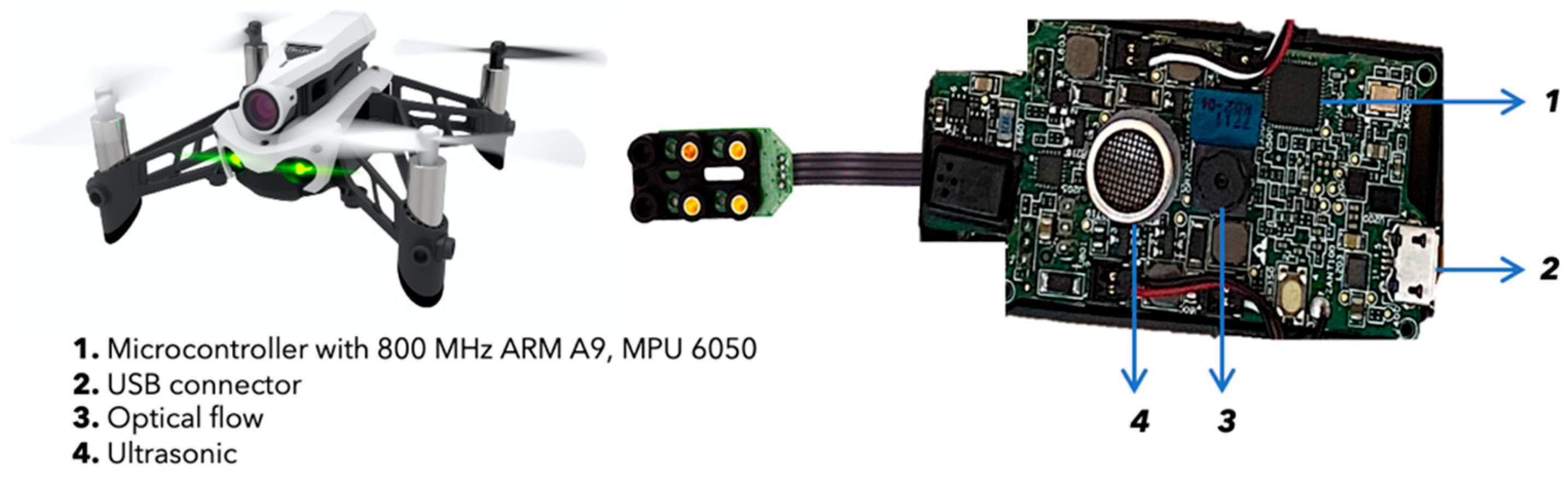
2.1. Parrot Mambo Sensors and Actuators
2.2. System Mathematical Modeling
- The quadcopter is treated as a rigid body with a symmetrical structure, facilitating a simplified yet robust characterization.
- The alignment of the center of gravity with the quadcopter’s geometrical center is assumed.
- Euler angles governing the orientation of the UAV () are constrained within specific bounds: , , and This constraint ensures realistic and physically meaningful variations in orientation.
- Both the position and velocity of the UAV are deemed measurable, providing essential parameters for accurate depiction of its motion.
- The thrust and drag forces are considered to be proportionally related to the squared velocity of the propellers, aligning with the principles of aerodynamics and motor dynamics.
- -
- and are, respectively, the model uncertainties and sensor measurement noise. They correspond to unmeasurable white noise that affects the model dynamics;
- -
- represents the total thrust force, while and are the total torque for roll, pitch, and yaw, respectively.
- -
- and are, respectively, linear and angular positions.
- -
- and are, respectively, linear and angular velocities.
- -
- To simplify the notation, we define = .
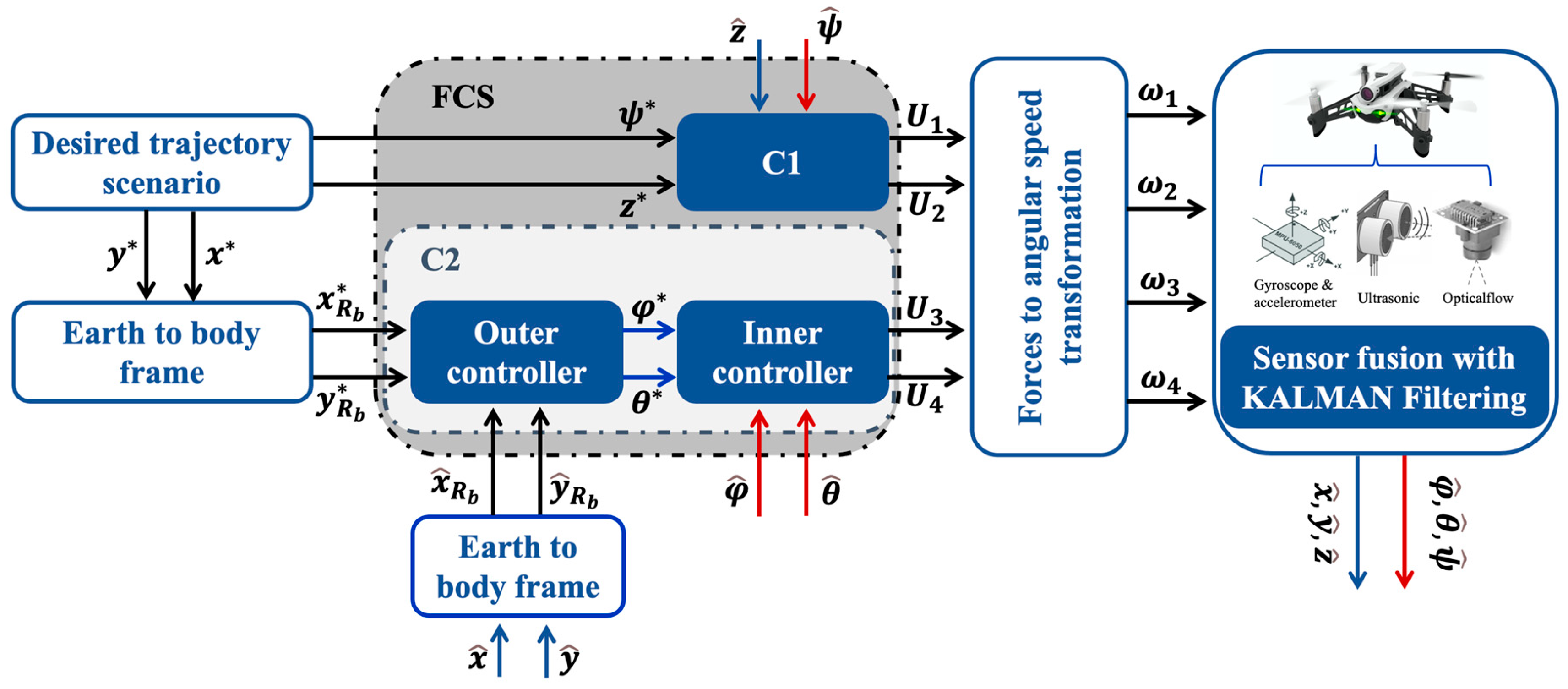
3. Controller Synthesis
3.1. Control Objectives
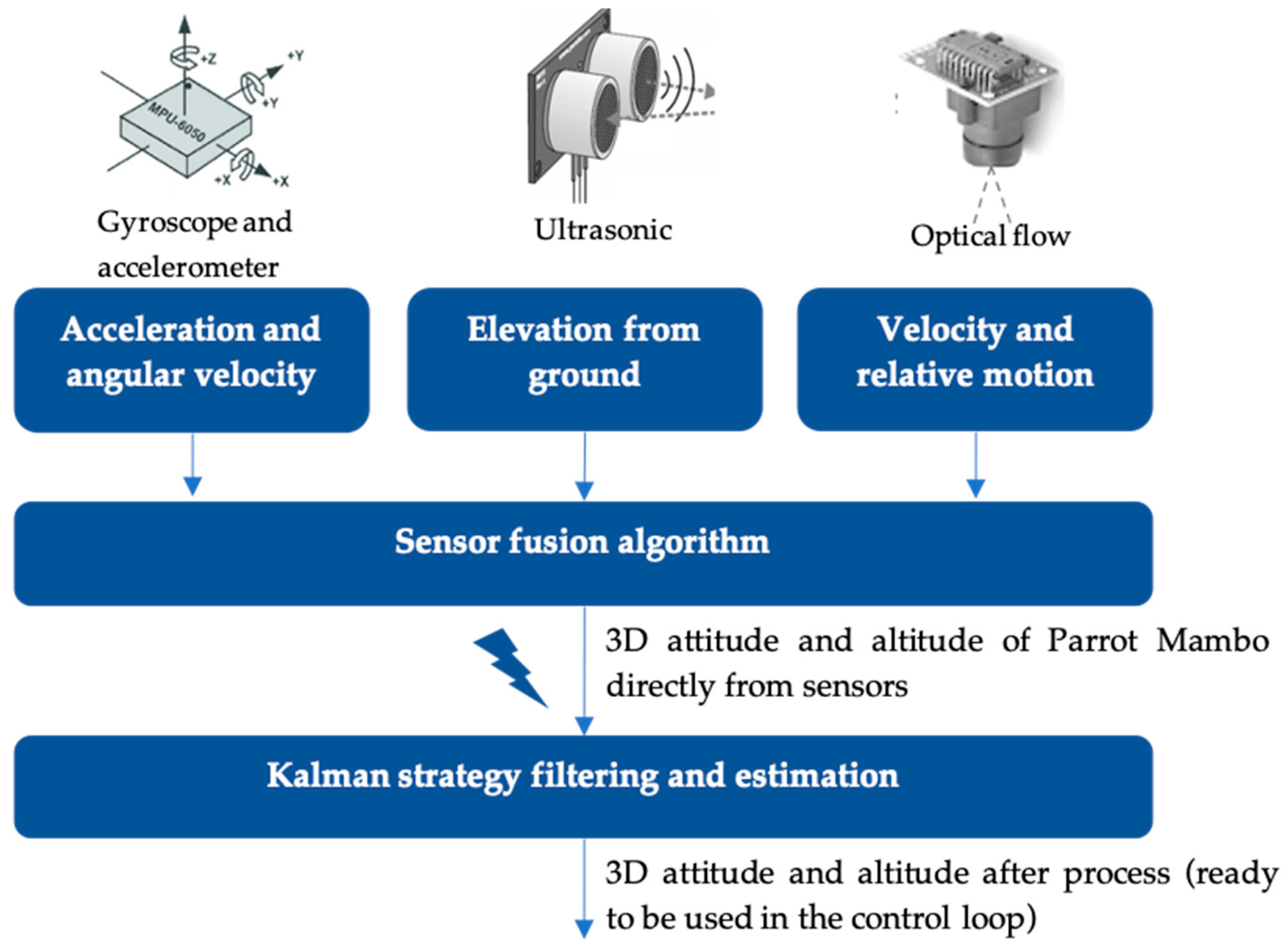
3.2. Sensor Fusion Algorithm
3.3. Overview and Synthesis of Kalman Filtering
3.3.1. Kalman Filtering in Drone Piloting
3.3.2. Extended Kalman Filter Synthesis
3.4. Control Strategy
- a.
- Inner Loop: Nonlinear Backstepping Control
- b.
- Outer loop: PID
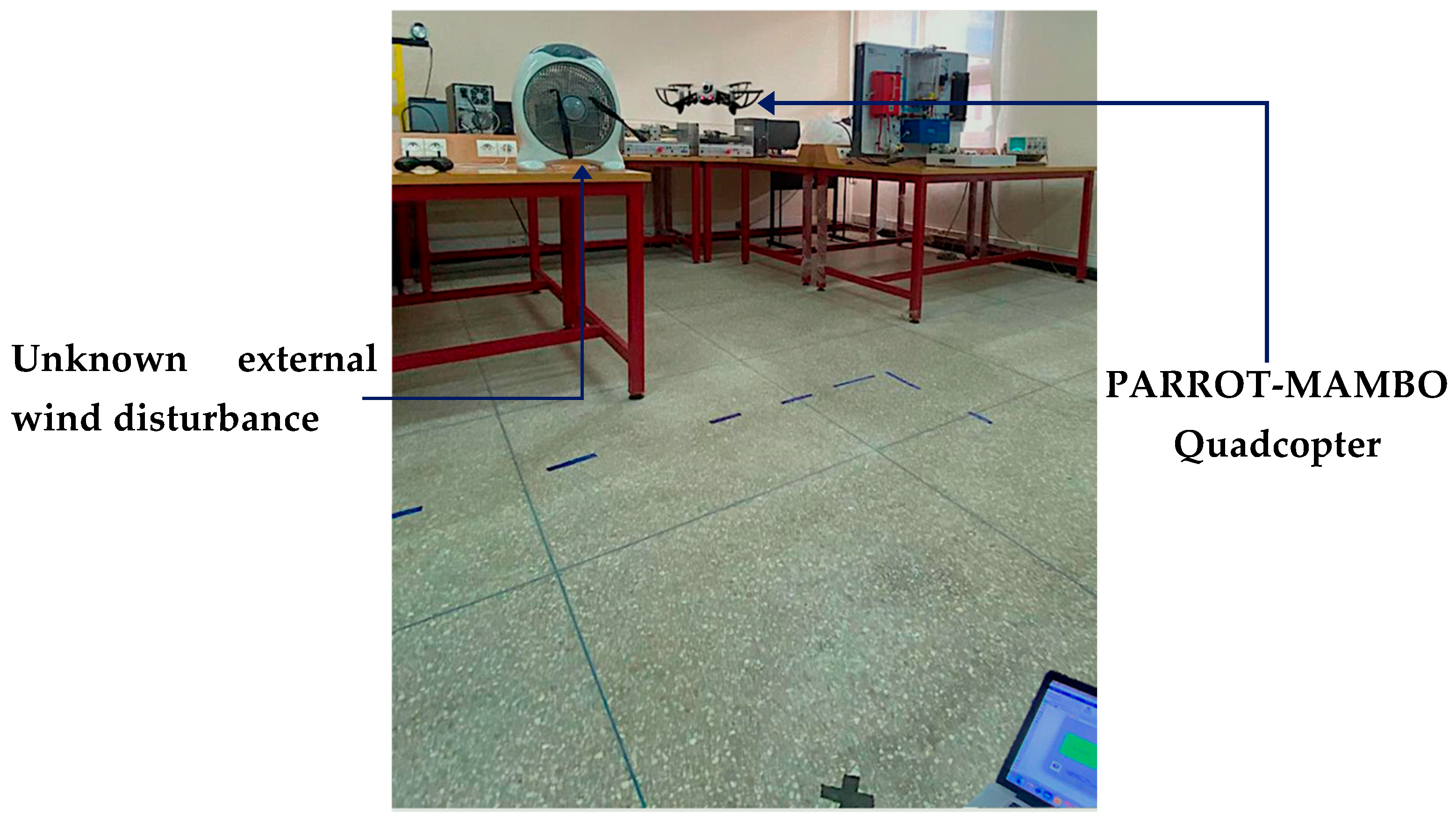
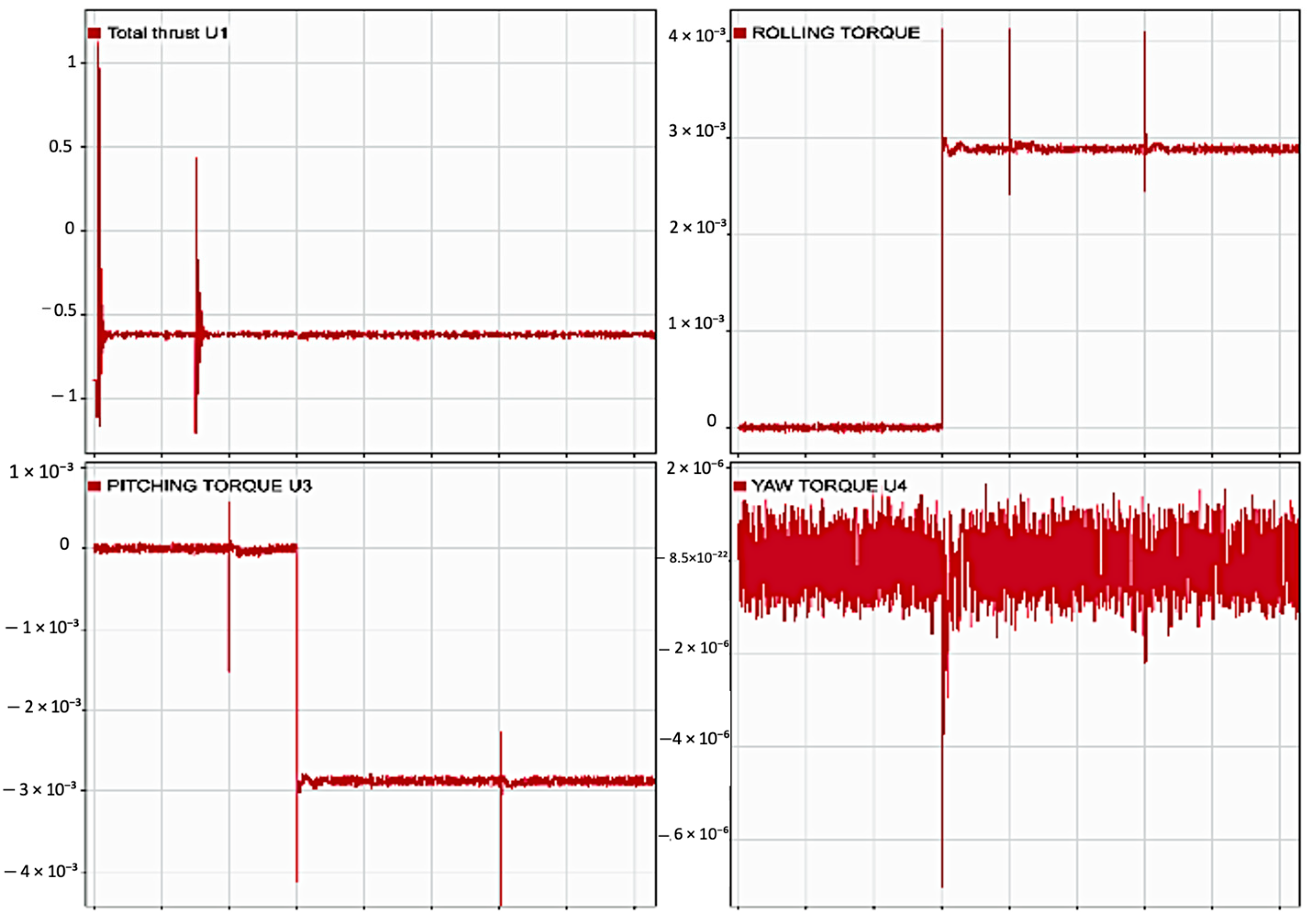
4. Results
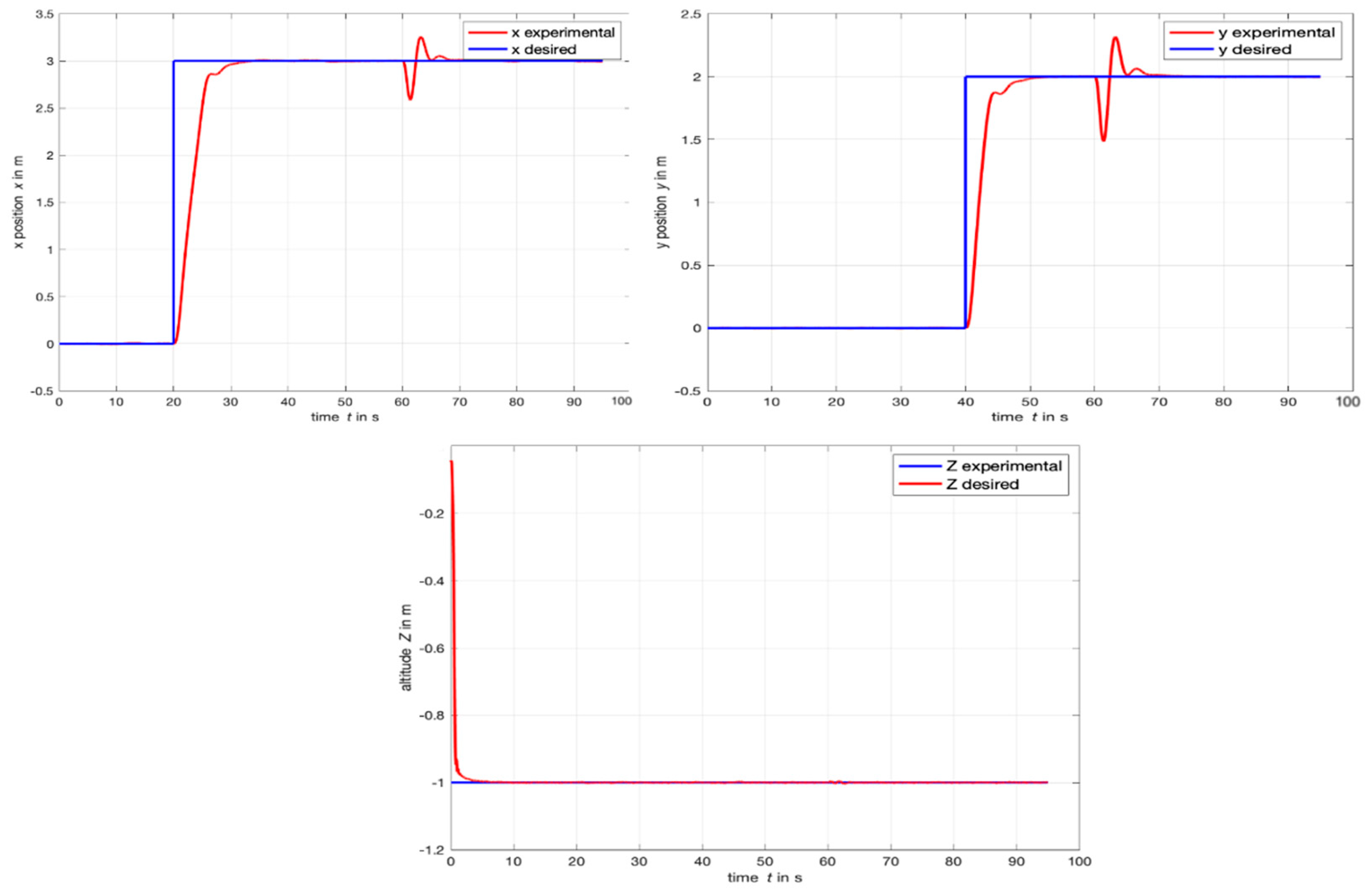
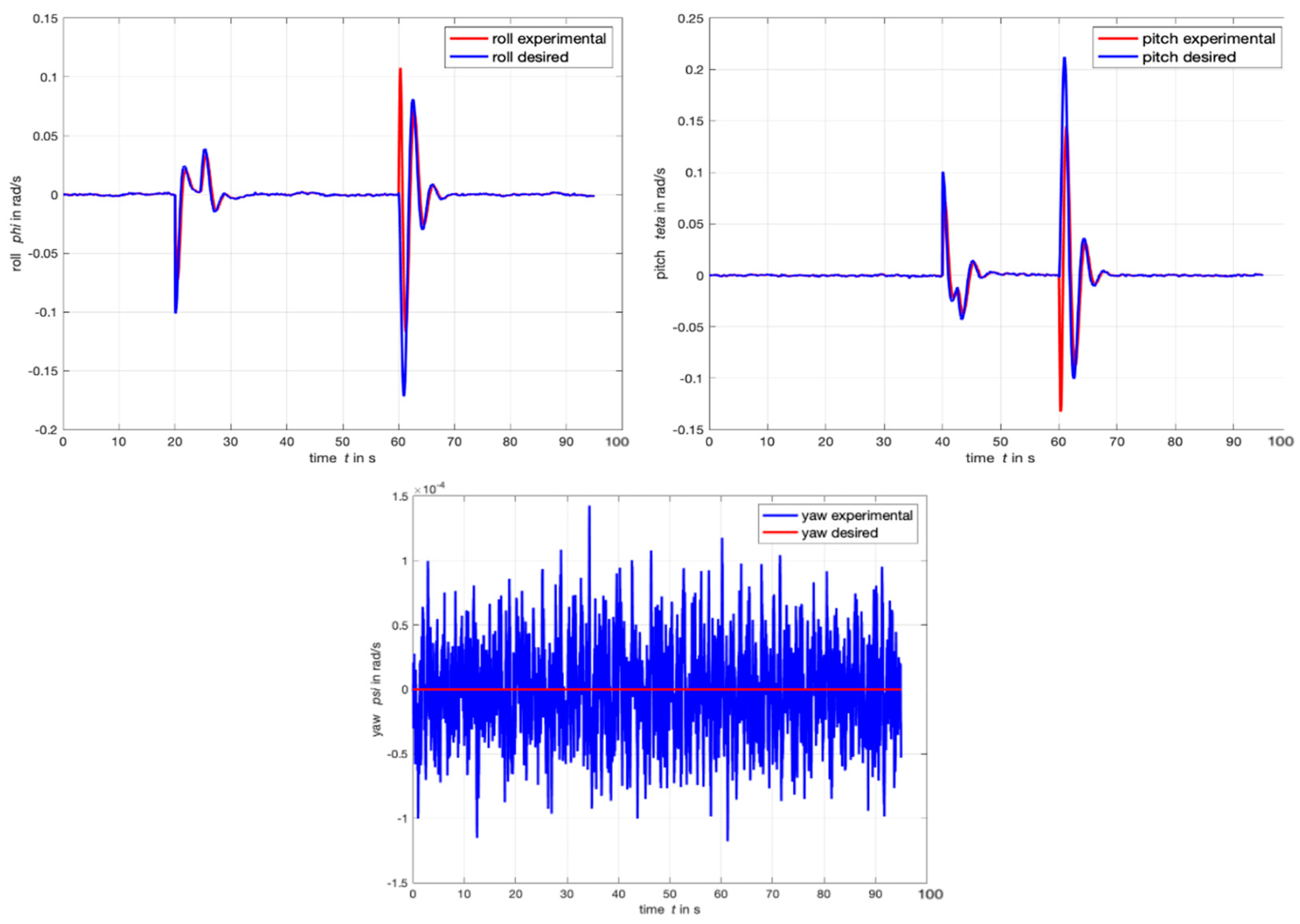
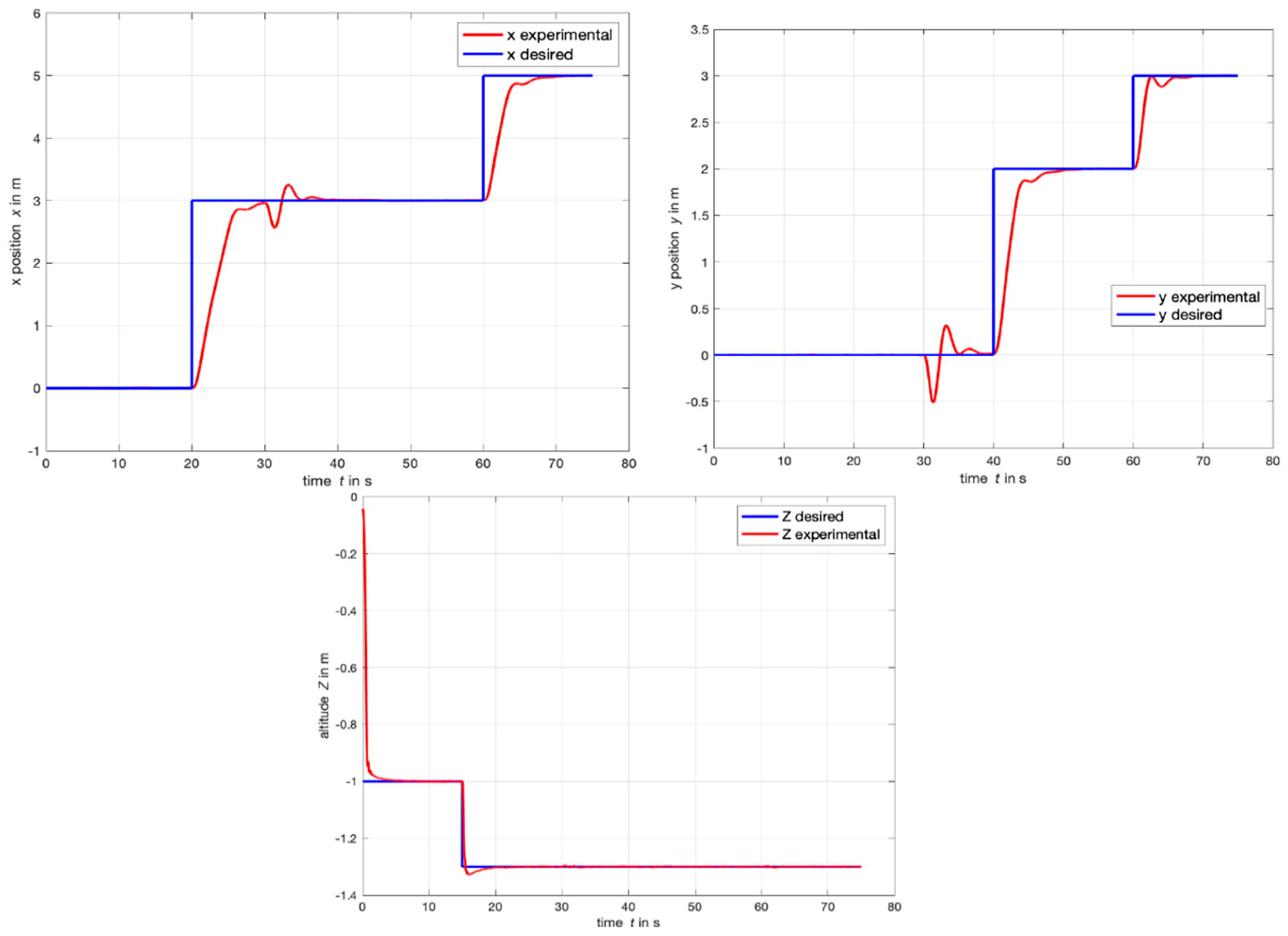
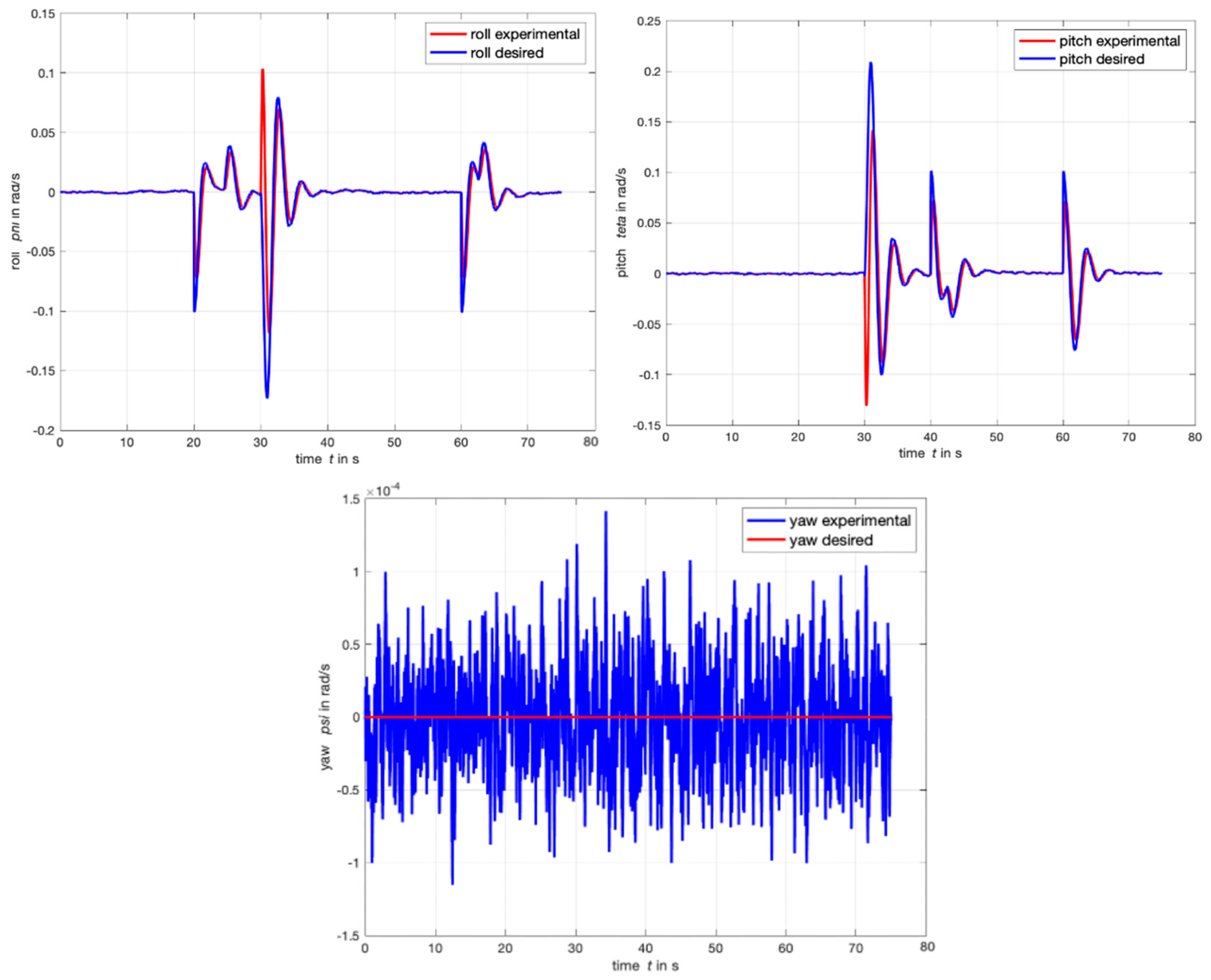
4.1. Step Response
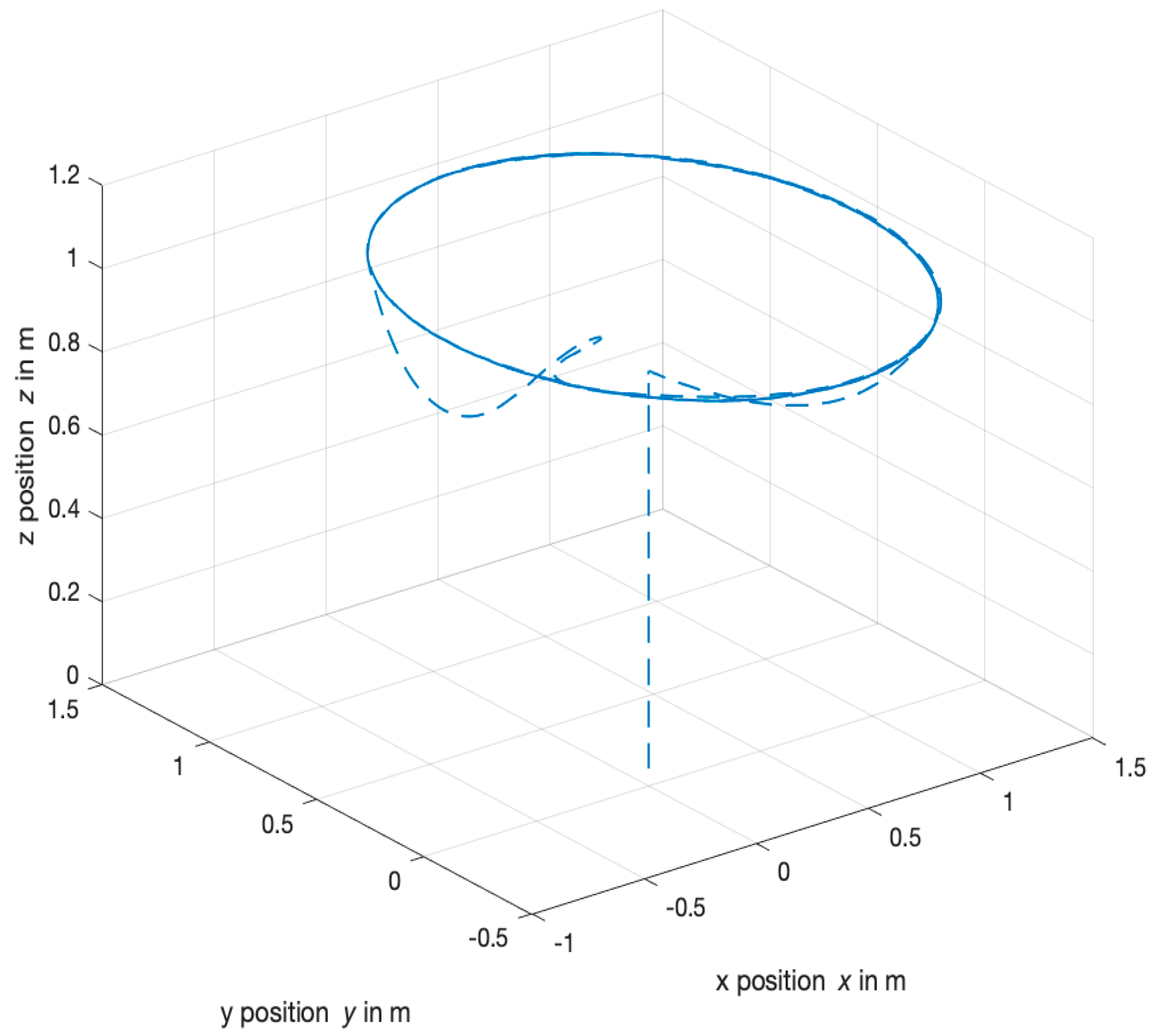
4.2. Orbit Response
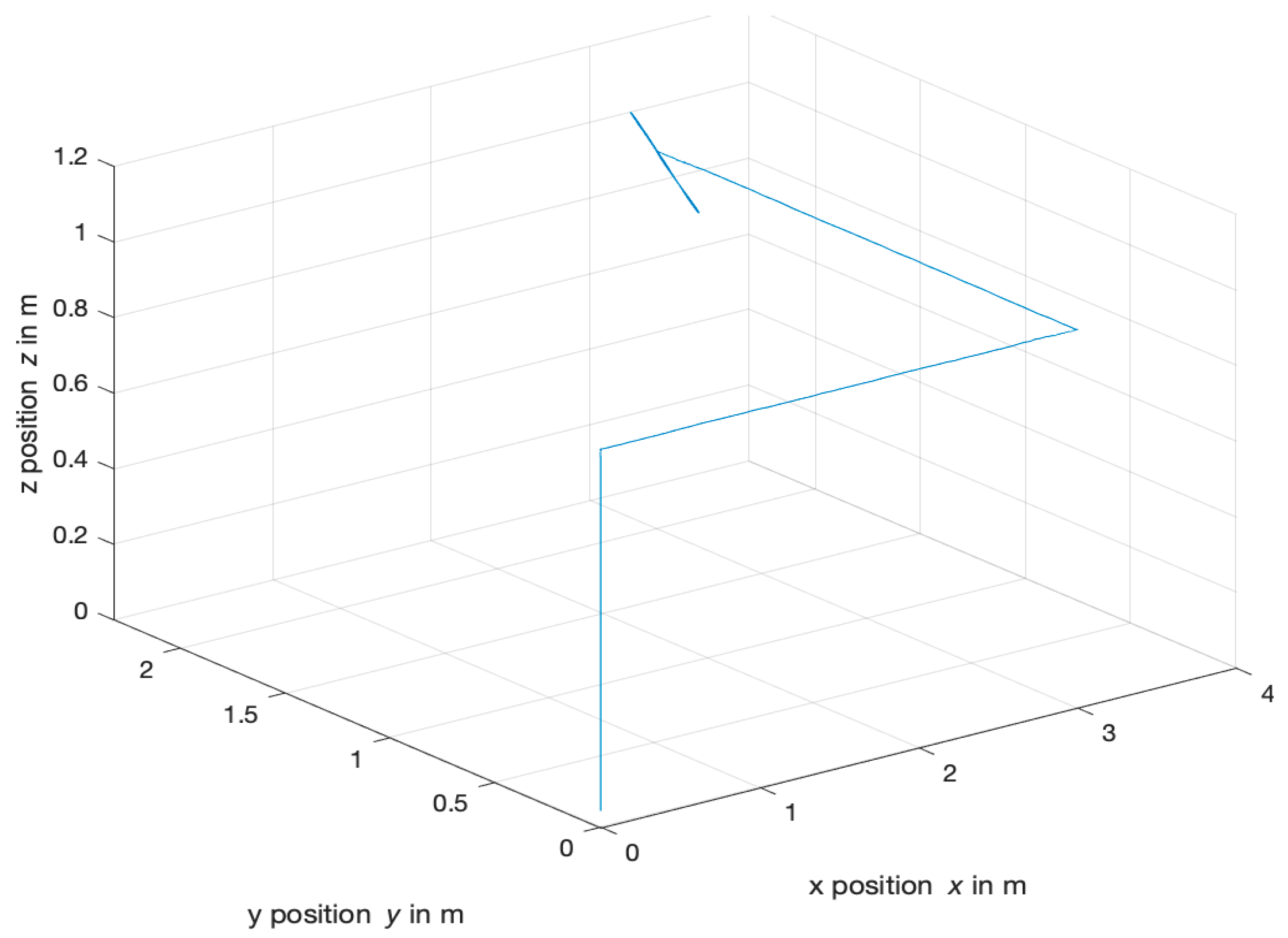
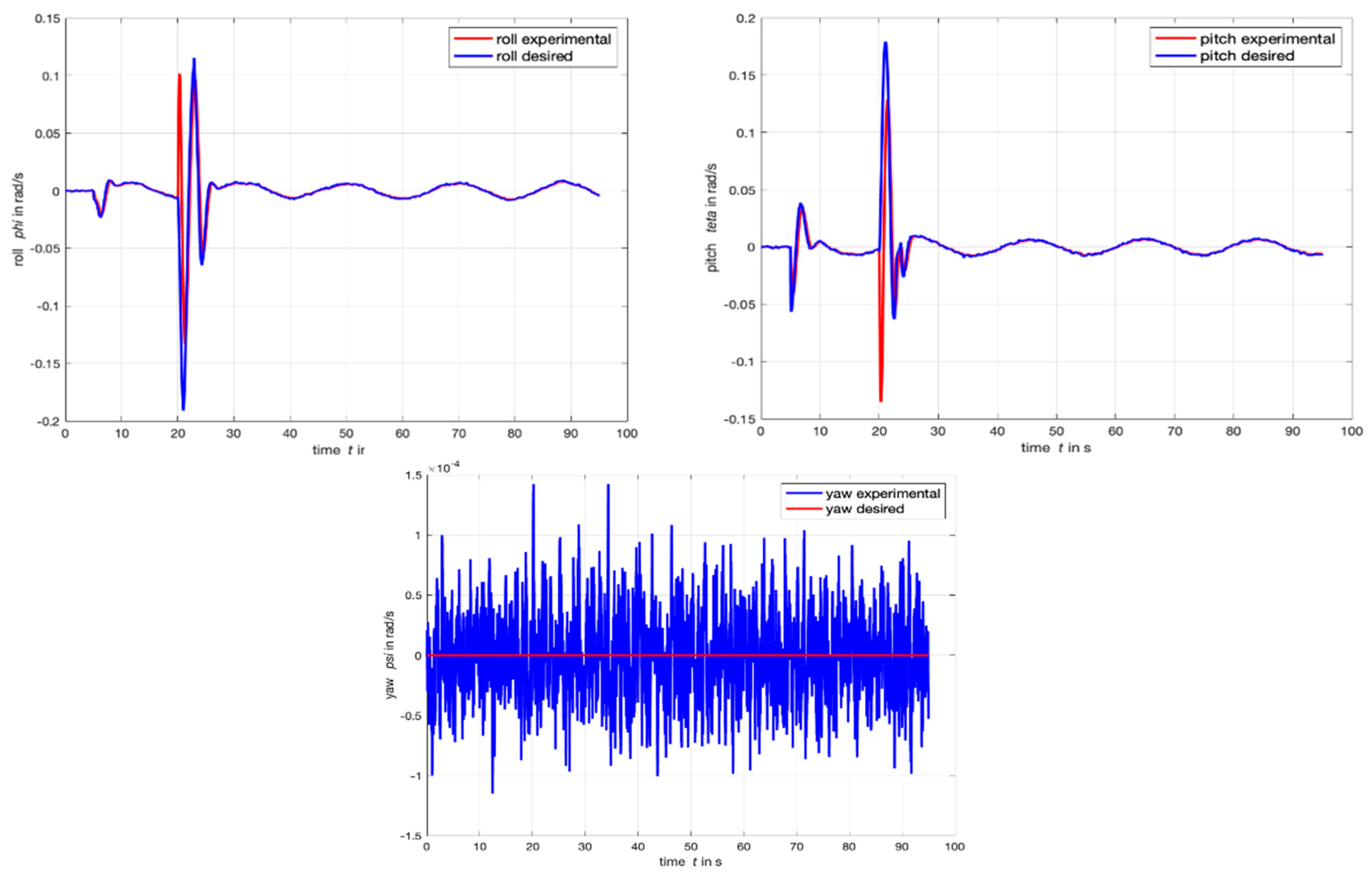
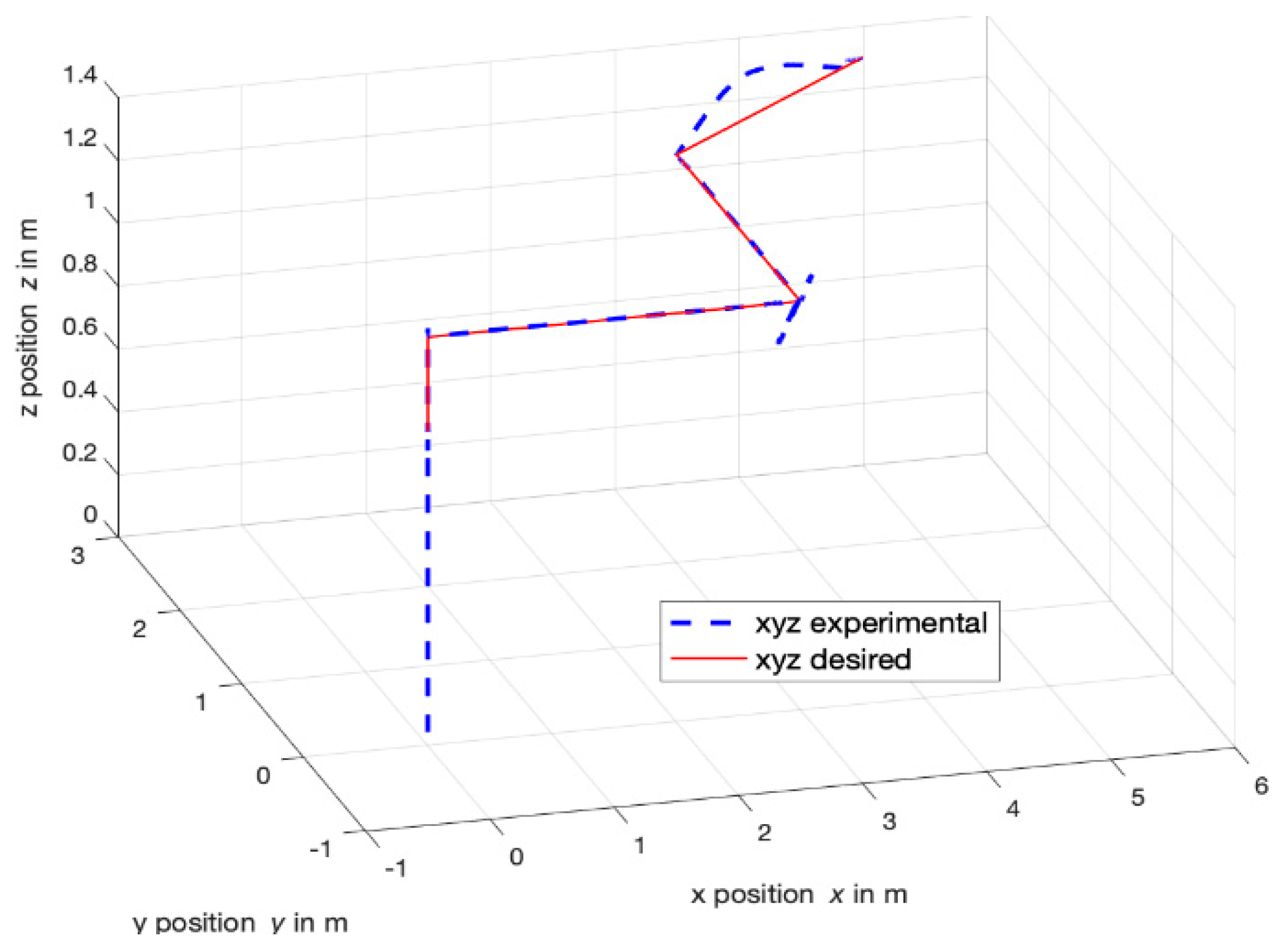
4.3. Waypoint Follower Response
5. Discussion
6. Conclusions
Author Contributions
Funding
Data Availability Statement
Acknowledgments
Conflicts of Interest
Abbreviations
| List of Acronyms | |
| ADRC | Active disturbance rejection control |
| BAP | Barometric air pressure |
| CBNC | Cascaded backstepping nonlinear controller |
| DOBC | Disturbance observer-based control |
| EKF | Extended Kalman filtering |
| ESO | Extended state observer |
| FCS | Flight control system |
| GPS | Global positioning system |
| IMU | Inertial measurement unit |
| LiPo | Lithium polymer |
| PID | Proportional integral derivative controller |
| PWR | Power-to-weight ratio |
| SKF | Standard Kalman filtering |
| TD | Tracking differentiator |
| UAV | Unmanned aerial vehicle |
| USB | Universal serial bus |
| Variables and Parameters | |
| φ, θ, ψ | Roll, pitch, yaw, respectively |
| x-coordinate measured along the east–west axis, y-coordinate measured along the north–south axis, and z-coordinate measuring elevation | |
| Quadrotor mass, | |
| , , | Rolling, pitching, and yawing moments of inertia, respectively, |
| Distance between the propeller axis and the mass center of the UAV in | |
| Translational drag coefficients in | |
| Aerodynamic friction coefficients in | |
| Thrust coefficient in and drag coefficient in , respectively | |
| Gravitational constant in | |
| Angular speed of motor in | |
| Rotor moment of inertia in | |
References
- Krstic, M.; Kanellakopoulos, I.; Kokotovic, P.V. Nonlinear design of adaptive controllers for linear systems. IEEE Trans. Autom. Control 1994, 39, 738–752. [Google Scholar] [CrossRef]
- Tripathi, V.K.; Behera, L.; Verma, N. Design of sliding mode and backstepping controllers for a quadcopter. In Proceedings of the 39th National Systems Conference (NSC), Greater Noida, India, 14–16 December 2015. [Google Scholar]
- Cho, M.G.; Jung, U.; An, J.-Y.; Choi, Y.-S.; Kim, C.-J. Adaptive trajectory tracking control for rotorcraft using incremental backstepping sliding mode control strategy. Int. J. Aerosp. Eng. 2021, 2021, 4945642. [Google Scholar] [CrossRef]
- Mouchrif, I.; Lachkar, I.; Abdelmajid, A.; Taame, A. ADRC control of an unmanned Under-Actuated aerial vehicle. In Lecture Notes in Electrical Engineering; Springer Nature: Singapore, 2024; pp. 1–13. [Google Scholar]
- Hu, Y.; Li, B.; Jiang, B.; Han, J.; Wen, C.-Y. Disturbance Observer-Based Model predictive control for an unmanned underwater vehicle. J. Mar. Sci. Eng. 2024, 12, 94. [Google Scholar] [CrossRef]
- Huang, S.; Xu, Z.; Cao, G.; Wu, C.; He, J. Nonlinear-disturbance-observer-based predictive control for trajectory tracking of planar motors. IET Electr. Power Appl. 2023, 18, 389–399. [Google Scholar] [CrossRef]
- Tang, X.; Zhao, F.; Tang, F.; Wang, H. Nonlinear extended Kalman filter for attitude estimation of the Fixed-Wing UAV. Int. J. Opt. 2022, 1–9. [Google Scholar] [CrossRef]
- Taame, A.; Lachkar, I.; Abouloifa, A.; Mouchrif, I. UAV altitude estimation using Kalman Filter and Extended Kalman Filter. In Lecture Notes in Electrical Engineering; Springer Nature: Singapore, 2024; pp. 817–829. [Google Scholar]
- Song, E.; Zhu, Y.; Zhou, J.; You, Z. Optimal Kalman filtering fusion with cross-correlated sensor noises. Automatica 2007, 43, 1450–1456. [Google Scholar] [CrossRef]
- Jwo, D.-J.; Biswal, A. Implementation and Performance Analysis of Kalman Filters with Consistency Validation. Mathematics 2023, 11, 521. [Google Scholar] [CrossRef]
- Noordin, A.; Basri, M.A.M.; Mohamed, Z. Real-Time implementation of an adaptive PID controller for the Quadrotor MAV embedded flight control system. Aerospace 2023, 10, 59. [Google Scholar] [CrossRef]
- Berghout, T.; Benbouzid, M. Fault Diagnosis in Drones via Multiverse Augmented Extreme Recurrent Expansion of Acoustic Emissions with Uncertainty Bayesian Optimisation. Machines 2024, 12, 504. [Google Scholar] [CrossRef]
- Reineking, T. Particle filtering in the Dempster–Shafer theory. Int. J. Approx. Reason. 2011, 52, 1124–1135. [Google Scholar] [CrossRef]
- Negru, S.A.; Geragersian, P.; Petrunin, I.; Guo, W. Resilient Multi-Sensor UAV Navigation with a Hybrid Federated Fusion Architecture. Sensors 2024, 24, 981. [Google Scholar] [CrossRef] [PubMed]
- Al-Absi, M.A.; Fu, R.; Kim, K.-H.; Lee, Y.-S.; Al-Absi, A.A.; Lee, H.-J. Tracking unmanned aerial vehicles based on the Kalman filter considering uncertainty and error aware. Electronics 2021, 10, 3067. [Google Scholar] [CrossRef]
- Pachter, M.; Chandler, P.R. Universal linearization concept for extended Kalman filters. IEEE Trans. Aerosp. Electron. Syst. 1993, 29, 946–962. [Google Scholar] [CrossRef]
- Harikrishnan, S.; Sulficar, A.; Desai, V. Hovering control of a quadcopter using linear and nonlinear techniques. Int. J. Mechatron. Autom. 2018, 6, 120–129. [Google Scholar]
- Sheta, A.; Braik, M.; Maddi, D.R.; Mahdy, A.; Aljahdali, S.; Turabieh, H. Optimization of PID Controller to Stabilize Quadcopter Movements Using Meta-Heuristic Search Algorithms. Appl. Sci. 2021, 11, 6492. [Google Scholar] [CrossRef]
- Eltayeb, A.; Rahmat, M.F.A.; Basri, M.A.M.. Sliding mode control design for the attitude and altitude of the quadrotor UAV. Int. J. Smart Sens. Intell. Syst. 2020, 13, 1–13. [Google Scholar] [CrossRef]
- Xiao, J. Trajectory planning of quadrotor using sliding mode control with extended state observer. Meas. Control 2020, 53, 1300–1308. [Google Scholar] [CrossRef]


| Parameter | Value |
|---|---|
Disclaimer/Publisher’s Note: The statements, opinions and data contained in all publications are solely those of the individual author(s) and contributor(s) and not of MDPI and/or the editor(s). MDPI and/or the editor(s) disclaim responsibility for any injury to people or property resulting from any ideas, methods, instructions or products referred to in the content. |
© 2025 by the authors. Published by MDPI on behalf of the International Institute of Knowledge Innovation and Invention. Licensee MDPI, Basel, Switzerland. This article is an open access article distributed under the terms and conditions of the Creative Commons Attribution (CC BY) license (https://creativecommons.org/licenses/by/4.0/).
Share and Cite
Taame, A.; Lachkar, I.; Abouloifa, A.; Mouchrif, I.; Aroudi, A.E. Nonlinear Output Feedback Control for Parrot Mambo UAV: Robust Complex Structure Design and Experimental Validation. Appl. Syst. Innov. 2025, 8, 95. https://doi.org/10.3390/asi8040095
Taame A, Lachkar I, Abouloifa A, Mouchrif I, Aroudi AE. Nonlinear Output Feedback Control for Parrot Mambo UAV: Robust Complex Structure Design and Experimental Validation. Applied System Innovation. 2025; 8(4):95. https://doi.org/10.3390/asi8040095
Chicago/Turabian StyleTaame, Asmaa, Ibtissam Lachkar, Abdelmajid Abouloifa, Ismail Mouchrif, and Abdelali El Aroudi. 2025. "Nonlinear Output Feedback Control for Parrot Mambo UAV: Robust Complex Structure Design and Experimental Validation" Applied System Innovation 8, no. 4: 95. https://doi.org/10.3390/asi8040095
APA StyleTaame, A., Lachkar, I., Abouloifa, A., Mouchrif, I., & Aroudi, A. E. (2025). Nonlinear Output Feedback Control for Parrot Mambo UAV: Robust Complex Structure Design and Experimental Validation. Applied System Innovation, 8(4), 95. https://doi.org/10.3390/asi8040095