Abstract
In the rapid process of urbanization, urban agglomerations have become a key driving factor for regional development and spatial reorganization. The formation and development of urban agglomerations rely on communication between cities. However, the spatiotemporal characteristics of intercity travelers are not fully grasped throughout the entire trip chain. This study proposes a spatiotemporal analysis method for intercity travel in urban agglomerations by constructing origin-to-destination (OD) trip chains using smartphone data, with the Beijing–Tianjin–Hebei urban agglomeration as a case study. The study employed Cramer’s V and Spearman correlation coefficients for multivariate feature selection, identifying 12 key variables from an initial set of 20. Then, optimal cluster configuration was determined via silhouette analysis. Finally, the K-prototypes algorithm was applied to cluster 161,797 intercity trip chains across six transportation corridors in 2019 and 2021, facilitating a comparative spatiotemporal analysis of travel patterns. Results show the following: (1) Intercity travelers are predominantly males aged 19–35, with significantly higher weekday volumes; (2) Modal split exhibits significant spatial heterogeneity—the metro predominates in Beijing while road transport prevails elsewhere; (3) Departure hubs’ waiting times increased significantly in 2021 relative to 2019 baselines; (4) Increased metro mileage correlates positively with extended intra-city travel distances. The results substantially contribute to transportation planning, particularly in optimizing multimodal hub operations and infrastructure investment allocation.
1. Introduction
Urban agglomerations have emerged as pivotal engines for regional economic growth and spatial reorganization in the context of accelerating global urbanization [1,2]. These agglomerations facilitate regional integration through resource consolidation, industrial synergy, and population concentration [3,4]. In China, strategic initiatives such as the Transport Power Construction Outline [5] and the 14th Five-Year Plan for Transportation Development [6] underscore the imperative to develop integrated transportation networks within urban agglomerations. Priorities include enhancing multimodal connectivity, advancing intelligent infrastructure, and optimizing intercity travel efficiency to foster coordinated regional development [7]. However, these objectives are impeded by multifaceted challenges, including inefficiencies in transportation systems and environmental capacity limitations [8]. In this context, analyzing intercity travel characteristics has become a critical approach for optimizing transportation planning and enhancing residents’ quality of life [9]. Intercity trip chains, functioning as dynamic networks linking nodes within agglomerations, not only capture spatiotemporal mobility behaviors but also inform data-driven strategies for resource allocation and multimodal optimization [10,11]. The COVID-19 pandemic has further reshaped mobility trends, underscoring the urgency of continuous monitoring and adaptive strategies to address evolving travel demands [12,13]. Due to the pandemic, in Spain, travel volume dropped dramatically while public transportation was extremely affected and private cars were relatively less affected [14]. The travel volume in most countries decreased [15,16]. The number of travelers who travelled for education, to visit friends, and for personal care decreased the most among all the purposes for travel in the Netherlands [17]. In China’s Greater Bay Area, it was found by analyzing mobile phone data that, in comparison to advantaged groups, socially disadvantaged groups experienced a steeper decline in travel mobility during the pandemic’s peak but a more significant recovery afterward [18].
Previous studies have achieved significant progress in analyzing intercity travel characteristics. Smart card data, valued for their accessibility and wide availability, have become a predominant big-data source in public transit research, enabling analyses of spatiotemporal commuting patterns and large-scale demand modeling [19]. When integrated with GPS trajectories, these data can reconstruct detailed trip sequences, though inferring trip purposes remains challenging [20]. To address this, Minimum Entropy Rate (MER) methods optimize sequence uncertainty and enhance origin–destination estimation [21]. Machine learning techniques (e.g., sequence alignment, decision trees) further identify recurrent mobility patterns in transit datasets [22,23], while discrete choice models quantify mode selection dynamics and comfort trade-offs in trip chains [24]. Concurrently, investigations into high-speed rail network development and its spatial interactions with urban agglomerations [25], along with analyses of multimodal travel decision-making processes [26], have significantly advanced theoretical frameworks for regional transportation planning. Despite these achievements, there are still some limitations. While traditional survey instruments effectively capture detailed trip characteristics, including purpose and mode choice [27], their implementation faces practical challenges, including substantial costs, limited spatial coverage, and low response rates, hindering their ability to represent population-wide mobility patterns at the urban agglomeration scale [28]. Furthermore, insufficient coverage of transient populations and non-commuting trips exacerbates sampling biases. From an analytical perspective, conventional clustering methods (e.g., K-means, K-modes) demonstrate limited efficacy when processing mixed data types, frequently producing suboptimal classifications due to their inability to effectively handle heterogeneous variables [29]. Current variable selection methods, often relying on simplified correlation measures, fail to adequately capture complex relationships between categorical and numerical features [30]. Additionally, the sensitivity of clustering algorithms to initialization parameters frequently results in locally optimal solutions [31]. Perhaps most significantly, prevailing research paradigms tend to examine transportation modes in isolation or focus on static spatial–temporal parameters, neglecting the dynamic interactions between multimodal systems, temporal fluctuations, and individual behavioral variations [26,32].
This study proposes the K-prototypes clustering framework for comprehensive trip chain analysis, addressing two key research gaps: incomplete trip chain data acquisition and information loss in reconstruction. The methodology integrates three technical innovations: (1) mobile signaling data for complete origin–destination chain generation, (2) an entropy-weighted mechanism to balance numerical and categorical variable contributions, and (3) the density peak theory for optimal cluster initialization. For feature selection, a novel hybrid approach combining Cramer’s V coefficient (for categorical associations) and Spearman’s rank correlation (for ordinal relationships) is implemented to identify the most discriminative variables characterizing intercity travel behavior patterns. The Beijing–Tianjin–Hebei urban agglomeration, a nationally strategic region with functional integration and a Beijing-centered multi-tiered transportation network, serves as an empirical testbed. The framework is empirically validated using the Beijing–Tianjin–Hebei metropolitan region as a case study, analyzing anonymized mobile signaling data (2019–2021) across six major corridors. A 12-variable dataset is analyzed through silhouette coefficient optimization, revealing critical insights into multimodal transfer dynamics, individual behavioral variations, and transportation hub performance. These findings provide valuable implications for urban mobility optimization and sustainable development strategies [33,34], demonstrating the framework’s effectiveness in complex urban transportation analysis.
The rest of the paper is organized as follows: Section 2 provides an overview of the study area, data collection, and methodology for generating intercity trip chains, including the extraction and processing of smartphone data to capture spatiotemporal mobility behaviors. To address the aforementioned research questions, Section 3 details the analytical framework, encompassing variable selection using the Cramer’s V–Spearman correlation coefficient method; determination of the optimal number of clusters via the Silhouette Coefficient; and the application of the K-prototypes algorithm for clustering mixed data types. Section 4 presents a discussion of the results, comparing temporal and spatial characteristics of intercity trip chains across different directions and years, while contextualizing the findings within the broader literature on urban mobility and transportation planning. Section 5 concludes the paper with highlights of the theoretical contributions.
2. Study Area and Trip Chain Data
2.1. Study Area
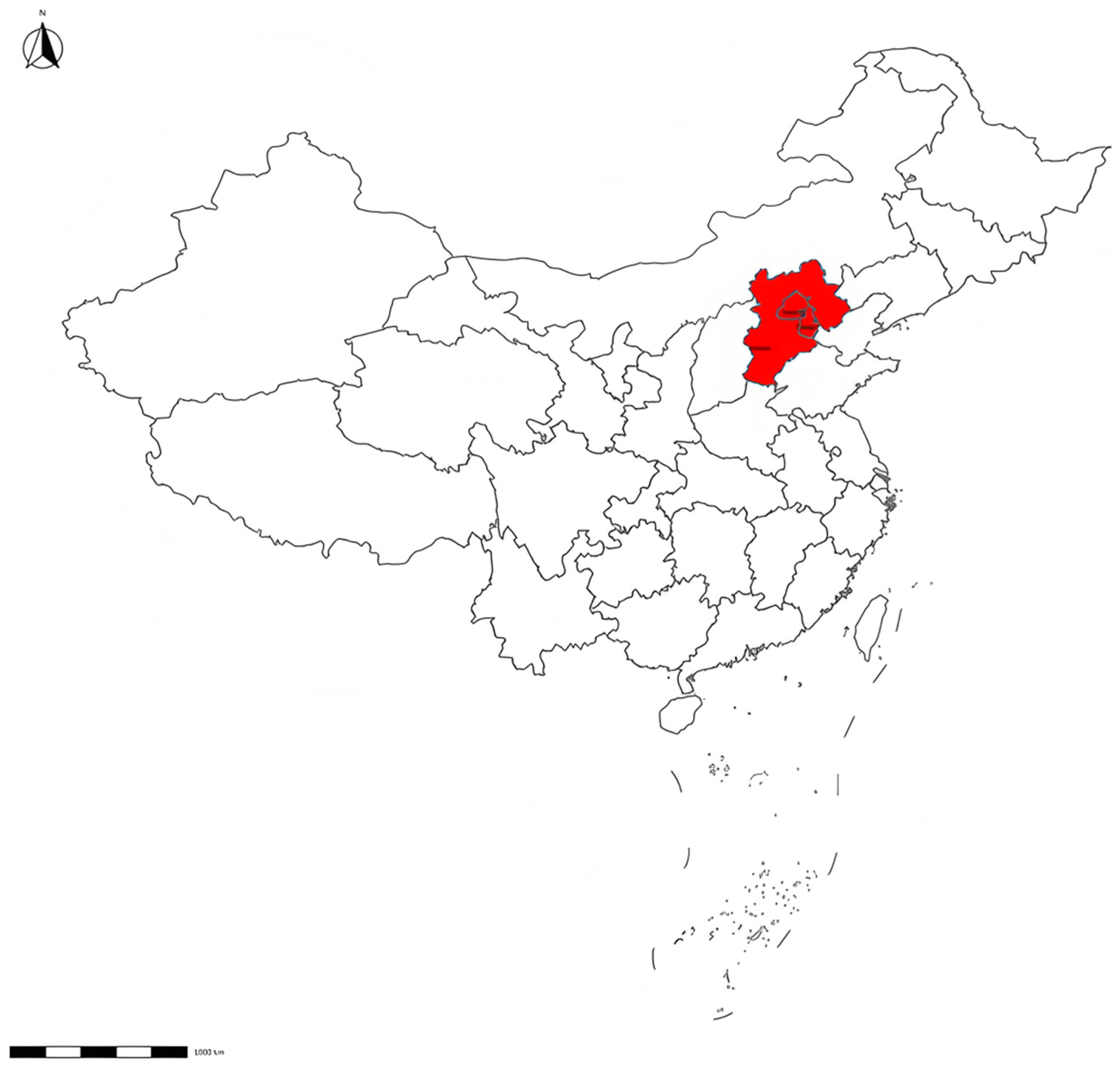
The Beijing–Tianjin–Hebei urban agglomeration is one of the four important international terminal clusters in China’s comprehensive national transport network [35]. Moreover, it serves as a capital economic circle and holds significant importance as the political and cultural center, contributing significantly to China’s development. Beijing is the political center of the China [36], gathering top research institutions and universities in China [37]. Eight major railway stations, including Beijing Station and Beijing South Station, are connected to the national high-speed rail network [38]. The Beijing–Tianjin intercity railway will achieve 5–10 min public transportation operation [39]. The operating mileage of the subway exceeded 727 km in 2024, making it one of the most densely populated rail transit networks in the world [40]. Tianjin is the core area of northern international shipping, with hubs such as Tianjin Station and Binhai Station connecting the Beijing–Shanghai and Tianjin–Qinhuangdao high-speed railways [41]. The subway mileage of Tianjin was about 233 km in 2024. Shijiazhuang is the capital of Hebei Province, undertaking Beijing’s non-capital function [42]. The subway mileage of Shijiazhuang was 76.5 km in 2024. The three cities are the three most important cities in the urban agglomeration [43]. Meanwhile, the intercity communication between Beijing, Tianjin, and Shijiazhuang is the most frequent within the urban agglomeration. Therefore, this study investigated the travel behavior of travelers using the high-speed railway for intercity travel between Beijing, Tianjin, and Shijiazhuang, within the Beijing–Tianjin–Hebei urban agglomeration as shown in Figure 1. The red part in Figure 1 represents the location of Beijing–Tianjin–Hebei urban agglomeration in China.

Figure 1.
Study area: Beijing–Tianjin–Hebei urban agglomeration.
2.2. Trip Chain Data
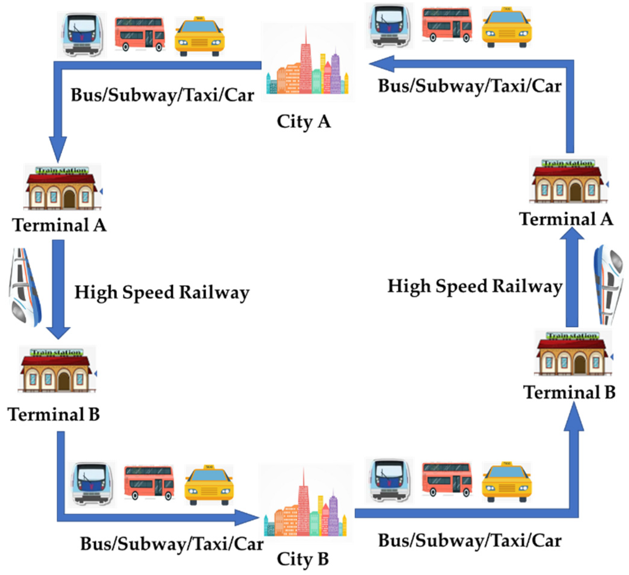
In this study, a trip chain refers to the whole process of intercity travel [44], which includes travel within the origin city, intercity travel by using a high-speed railway, and travel within the destination city, as shown in Figure 2. Regarding the travel process from City A to Terminal A, travelers departing from Beijing have longer travel distances and are more likely to choose subway transportation [45], because Beijing has the largest urban area and the longest subway mileage among the three cities. Regarding the intercity travel process using a high-speed railway, it takes 30 min between Beijing and Tianjin, 80 min between Beijing and Shijiazhuang, and 130 min between Tianjin and Shijiazhuang. Regarding the travel process from Terminal B to City B, travelers arriving at Beijing experience the most developed public transportation system and congested roads. The travel process from City B to City A has the same pattern as the travel process from City A to City B. A trip chain contains a lot of information, such as travel time, space trajectory, mode of transportation, and so on, and is accompanied by the whole process of travel.
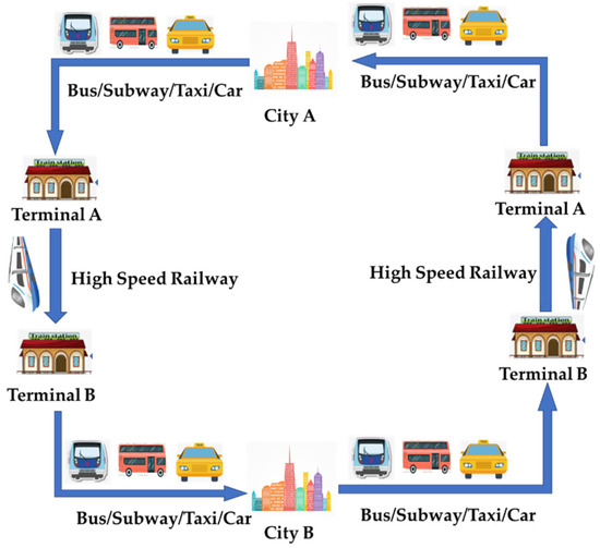
Figure 2.
Schematic diagram of urban agglomeration trip chain.
The raw data used to generate trip chains is smartphone data, and it is collected from the platform of Data-as-a-Service (DAAS) which is operated by one of the Chinese communication operators with a 30% market share within the Beijing–Tianjin–Hebei urban agglomeration. Based on this smartphone data, the intercity trip chains between three cities were extracted through three steps: identifying intercity travelers, extracting travel features within the city, and generating intercity trip chains [46]. There are 19 variables included in the trip chains as shown in Table 1.

Table 1.
Description of trip chain data variables.
This study analyzed intercity travel data for May 2019 and May 2021, which are before the outbreak of COVID-19 and the period of the post-COVID-19 phase, respectively. Unlike other countries, Chinese residents resumed travel, and the tourism industry was gradually recovering since April 2020 [47]. China had entered into a special and unique recovering period that was distinct from the other countries that were still experiencing serious impacts from COVID-19. China observes a five-day holiday in May for Labor Day, but it does not include longer breaks like winter or summer vacations that can cause changes in daily travel patterns. May also offers a favorable climate for travel [48]. Therefore, the data includes holidays, weekends, and workdays simultaneously and is representative to some extent. This study collected a total of twelve datasets from six directions over 2 years, amounting to 161,797 trip chains as shown in Table 2.
Table 2.
The data size.
3. Methods
In this study, the Cramer’s V–Spearman correlation coefficient method was used for variable selection [49]. The silhouette coefficient method was used to determine the number of clusters [50]. The K-prototypes algorithm was used to cluster intercity trip chains [51].
3.1. Variable Selection for Clustering Based on Cramer’s V—Spearman Correlation Coefficient
The trip chains data used in this study consist of twenty variables, and there are two main challenges if all of them are used for cluster analysis [52]. First, high dimensionality can lead to the “curse of dimensionality” during clustering. Second, significant correlations between variables may affect the accuracy and efficiency of the clustering process. To address these issues, a variable selection process is implemented to eliminate highly correlated variables while retaining those that significantly impact the clustering results [53].
Common methods for calculating correlation include Spearman’s correlation coefficient, the Pearson correlation coefficient, Cramer’s V coefficient, the chi-square test, and covariance. Spearman’s coefficient is suitable for categorical data or data that does not fully adhere to a normal distribution [54]. It is less sensitive to outliers and does not impose strict data requirements. Pearson’s coefficient is applicable for analyzing linear relationships between continuous variables, requiring normally distributed data and assuming linearity between variables [55]. Cramer’s V is used to assess correlations between discrete, unordered data [56]. The chi-square test primarily compares proportions among two or more samples and examines the association between categorical variables [57]. Covariance measures the relationship between two continuous random variables [58].
Because the twenty variables describing trip chains include both unordered categorical and numerical variables, a single method cannot calculate the correlation between all variables. Therefore, a combined method based on Cramer’s V and Spearman was applied in this study. The correlation coefficient between six unordered categorical variables, which were Weekday, Gender, Type-O, Type-D, Mode-O, and Mode-D, was calculated using the Cramer’s V coefficient method. In this study, as the numerical variables were grouped variables with a small range of values, they could be regarded as ordered categorical variables. Therefore, the Spearman method was applied to calculate correlations among numerical variables, as well as between unordered categorical and numerical variables. The specific calculation methods are outlined below:
- Cramer’s V coefficient method
Cramer’s V coefficient method was introduced by Karl Cramer in 1946 and is calculated based on Pearson’s chi-square statistics, considering the total sample size and degrees of freedom. The specific formula is as follows:
where χ2 is the chi-square statistic obtained from a contingency table formed by two categorical variables, n represents the total sample size, r is the number of categories for the first variable, c is the number of categories for the second variable, min (r − 1, c − 1) denotes the smaller of the two values derived from reducing the counts of each categorical variable by one, O indicates the observed frequency, and E signifies the expected frequency. The value of Cramer’s V coefficient ranges from 0 to 1. The value of Cramer’s V coefficient being less than 0.3 indicates a weak correlation between the two variables, while a value greater than 0.6 suggests a strong correlation.
- 2.
- Spearman correlation coefficient
The Spearman correlation coefficient is defined as the Pearson correlation coefficient for ordinal variables. For sample size n, the original data are transformed into ranks, and the correlation coefficient ρ is calculated as follows:
where is the i-th value of the variable x, is the average value of x, is the i-th value of the variable y, and is the average value of y. The absolute value of indicates the strength of the rank correlation between the two variables. A positive indicates a positive correlation, while a negative indicates a negative correlation. When = 1, it indicates a completely correlated relationship between the two variables. When is between 0.8 and 1, it indicates a strong correlation. When is between 0.5 and 0.8, it indicates a moderate correlation. When is between 0.3 and 0.5, it indicates a weak correlation. When is less than 0.3, it generally reflects a very weak correlation that can be nearly negligible.
3.2. Silhouette Coefficient Method
As an unsupervised learning algorithm, the K-prototypes algorithm requires an appropriate method to determine the number of clusters, that is, the value of K, which directly impacts the effectiveness of the clustering results. The elbow method [59] and silhouette coefficient [60] are mostly used to calculate the value of K. The elbow method is based on observing the trend of the sum of squared errors (SSE) across different K values to identify the optimal K value. However, the elbow method may be somewhat subjective in selecting the optimal K value, as the determination of the elbow point depends on the judgment of the observer [61]. In some instances, the decreasing trend of SSE may not be obvious, making it difficult to identify the elbow point. In contrast, the silhouette coefficient is generally considered to be more objective and accurate since it considers both cohesion and separation factors, measuring how similar a sample point is to other points in its cluster and how well it separates from different clusters [62]. Consequently, this study adopts the silhouette coefficient method to determine the optimal number of clusters K for the K-prototypes algorithm. The steps for calculating the silhouette coefficient are as follows:
Step 1: Select a point denoted as from cluster m. Within the same cluster, calculate the distances between point and all other points to identify the average of these distances within the cluster, which is , reflecting the intra-cluster cohesion of the m cluster, as shown in Equation (4), where is the total number of samples in cluster m.
Step 2: Let be the point in cluster c, j = 1, 2, …, . Calculate the average distance between and , and then identify the minimum average distance by traversing all other clusters, as outlined in Equation (5). This reflects the separation between clusters, where K is the number of clusters.
Step 3: The silhouette coefficient is determined by both inter-cluster dispersion and intra-cluster cohesion, as shown in Equation (6).
Step 4: Calculate the average silhouette coefficient of all sample data to obtain the overall silhouette coefficient. The value of the silhouette coefficient should range from 0 to 1. As it approaches 1, the clustering results are more in line with the actual situation.
3.3. K-Prototypes Algorithm
Since the variables involved in trip chains include both categorical data, such as gender and mode of transportation, as well as numerical data, such as travel distance and travel time, clustering methods like K-means for numerical data and K-modes for categorical data are no longer suitable for clustering trip chains in this study [63]. The K-prototypes algorithm is a well-established method for clustering mixed data types [64]. It builds upon the framework of the K-means algorithm while integrating features of the K-modes algorithm. By adjusting parameters, it balances the relative importance of categorical and numerical data during the clustering process. This approach is both simple and highly efficient, making it widely used in clustering tasks that involve mixed datasets.
Let denote the set of intercity trip chains, which comprise n pieces of data. Each is characterized by attribute , where the first attribute is numerical, and the subsequent attributes are categorical. Let denote the set of values for all attributes, where is the set of values for attribute , . When 1 ≤ j ≤ , corresponds to numerical values. When ≤ j ≤ m, corresponds to categorical values, , where is the number of categorical values for attribute . Let denote the set of clusters, where K is the number of clusters. denotes the proportion of value in cluster , as outlined in Equation (7).
Let denote the set of cluster centers, where is the center of cluster . For each center , the following conditions apply:
where denotes the most frequent value of attribute within cluster . The dissimilarity between and cluster center is calculated as follows:
where is the dissimilarity for numerical attributes, is the dissimilarity for categorical attributes, and is a weight that controls the contributions of numerical and categorical attributes. is defined as follows:
The objective function of the K-prototypes algorithm can be defined as follows:
The value of is 0 or 1, where 1 indicates that is assigned to cluster , and 0 indicates that is assigned to cluster . Each data is partitioned and assigned to only one cluster. In summary, the steps for implementing the K-prototypes algorithm are as follows:
Step 1: Randomly select K pieces of data from dataset as the initial cluster centers. The initial cluster center set is .
Step 2: Calculate the distance between and , which is the cluster center.
Step 3: According to the minimum value of , assign to the corresponding cluster where is located.
Step 4: After assigning all to the corresponding cluster, recalculate the cluster centers of each cluster based on the cluster updating method for numerical and categorical data.
Step 5: Repeat Step 2, Step 3, and Step 4 until the clustering criterion function converges.
Step 6: Finish the algorithm and generate the results.
4. Results and Discussion
4.1. Variable Selection
The correlation coefficient calculations were performed using IBM Statistical Package for the Social Sciences 26 on a Lenovo laptop with an Intel(R) Core (TM) i7-10750H 2.60 GHz CPU and 32.0 GB of RAM. To fairly compare the characteristics of different trip chain datasets, it is important to select the same variables to conduct clustering. Therefore, the twelve trip chain datasets were grouped for correlation analysis. In this study, Cramer’s V method is employed to analyze the relationships between six unordered categorical variables: Weekday, Gender, Type-O, Mode-O, Mode-D, and Type-D. The Spearman method is applied to analyze the remaining 13 variables and the correlations between the 6 categorical variables and the 13 variables. The results are as shown in Table 3.
Table 3.
Correlation coefficients of each attribute.
In Table 3, the correlation coefficients between the six variables, which are MOT-O, THub-O, De-O, THub-D, De-D, and MOT-D, are all greater than 0.9, with significance test p-values of less than 0.05, leading to the rejection of the null hypothesis and indicating a strong correlation among these variables [65]. Meanwhile, these six variables are all time-related variables, including departure time, arrival time, hub departure time, hub arrival time, and arrival time. Therefore, only one of them will be selected as the variable for clustering. Considering that the departure time from the origin is the starting point of the trip chain and determines the other five variables, MOT-O is selected for clustering. Table 3 shows that the correlation coefficient between DS-O and Tr-T-O is 0.754, and the correlation coefficient between DS-D and Tr-T-D is 0.758. Both results have passed the significance test and indicate a moderate correlation. Given that independent time-related variables are involved in this study and that transportation mode and travel distance can be used to estimate travel time, DS-O and DS-D are selected for clustering. In summary, this study selects 12 variables for clustering analysis: 6 categorical variables (Weekday, Gender, Type-O, Mode-O, Type-D, and Mode-D) and 6 numerical variables (Age, MOT-O, Ds-O, Wt-O, Wt-D, and Ds-D).
4.2. Optimal Number of Clusters
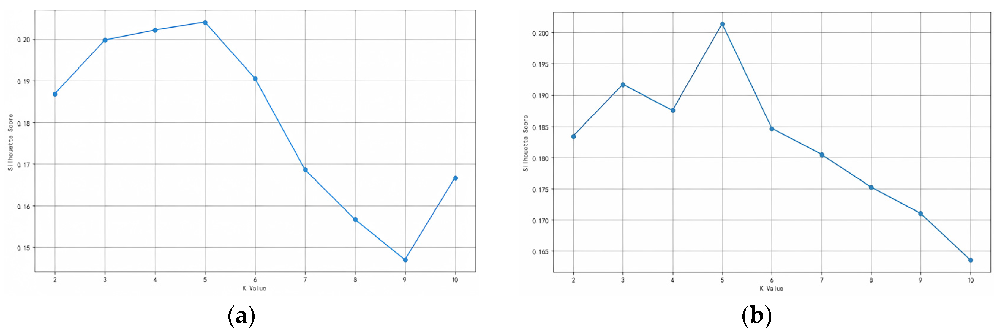
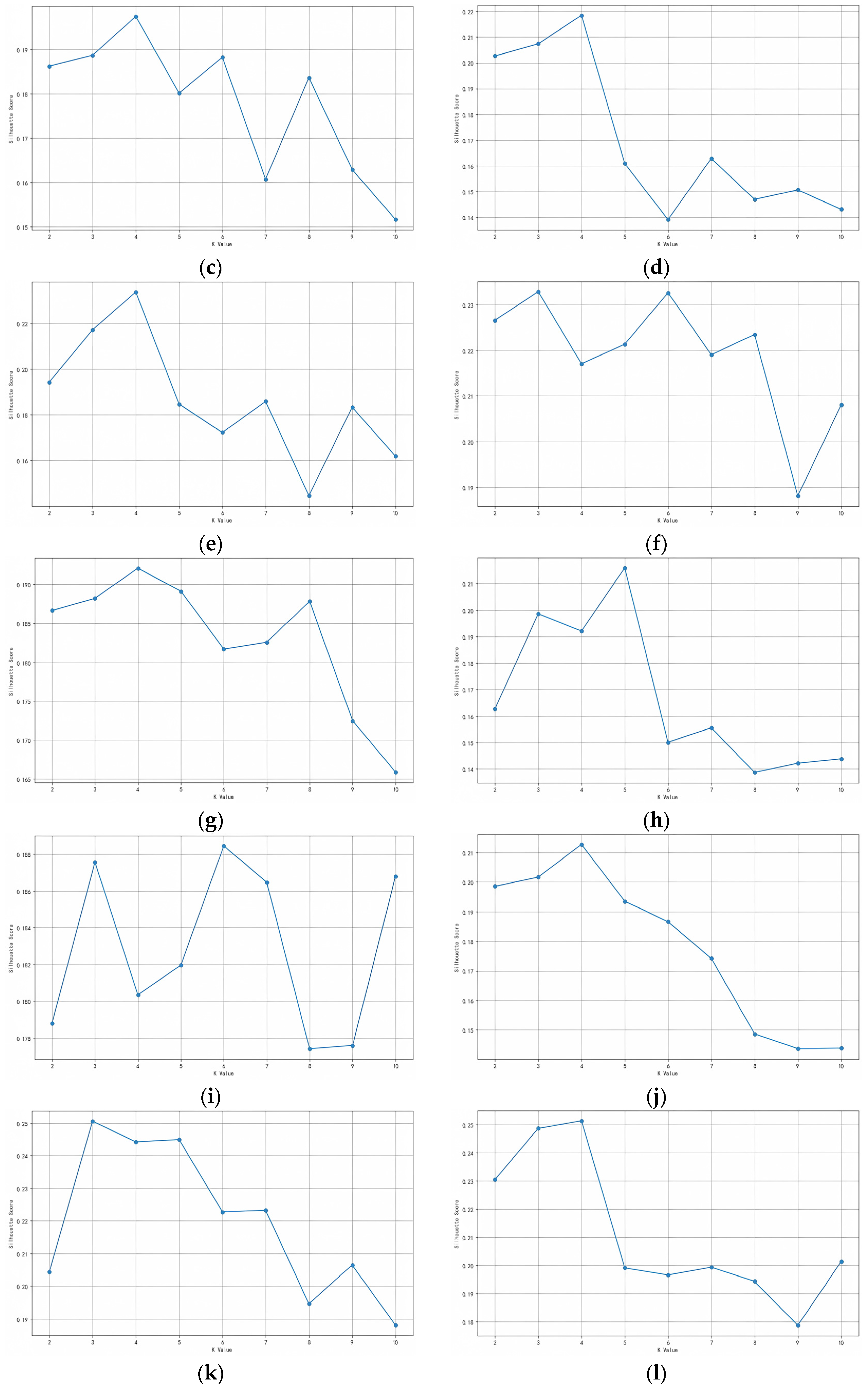
Based on the twelve trip chain datasets, the silhouette coefficient method is applied using the mathematical programming software Python 3.5 on a Lenovo laptop with an Intel(R) Core (TM) i7-10750H 2.60 GHz CPU and 32.0 GB of RAM to identify the optimal number of clusters. This study calculated the silhouette scores corresponding to cluster numbers K ranging from two to ten. The results are as shown in Figure 3.
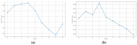
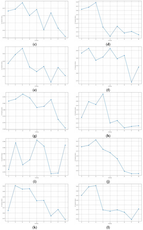
Figure 3.
(a) Silhouette coefficient of intercity trip chain from Beijing to Tianjin (May 2019); (b) Silhouette coefficient of intercity trip chain from Tianjin to Beijing (May 2019); (c) Silhouette coefficient of intercity trip chain from Beijing to Shijiazhuang (May 2019); (d) Silhouette coefficient of intercity trip chain from Shijiazhuang to Beijing (May 2019); (e) Silhouette coefficient of intercity trip chain from Tianjin to Shijiazhuang (May 2019); (f) Silhouette coefficient of intercity trip chain from Shijiazhuang to Tianjin (May 2019); (g) Silhouette coefficient of intercity trip chain from Beijing to Tianjin (May 2021); (h) Silhouette coefficient of intercity trip chain from Tianjin to Beijing (May 2021); (i) Silhouette coefficient of intercity trip chain from Beijing to Shijiazhuang (May 2021); (j) Silhouette coefficient of intercity trip chain from Shijiazhuang to Beijing (May 2021); (k) Silhouette coefficient of intercity trip chain from Tianjin to Shijiazhuang (May 2021); (l) Silhouette coefficient of intercity trip chain from Shijiazhuang to Tianjin (May 2021).
Figure 3 shows the results of silhouette coefficients corresponding to different cluster numbers K ranging from two to ten for twelve datasets. The numerical value of the silhouette coefficient is related to the clustering effect and the K value corresponding to the maximum silhouette coefficient is the optimal number of clusters. Based on the silhouette coefficients presented in Figure 3, the optimal number of clusters (optimal value of K) for intercity trip chains with six directions in two years is as shown in Table 4. The dataset with the highest number of clusters is Beijing–Shijiazhuang while the dataset with the least number of clusters is Tianjin–Shijiazhuang.
Table 4.
The optimal number of clusters for intercity trip chains.
4.3. Clustering Results Analysis
This study conducted a detailed comparative analysis of trip chains from temporal and spatial perspectives.
4.3.1. Comparative Analysis of Intercity Trip Chains from a Temporal Perspective
Table 5 shows the most frequently clustering centers of intercity trip chains between Beijing and Tianjin in May 2019 and May 2021. In the Beijing to Tianjin direction, the age distribution of travelers changed from 25–29 years old in 2019 to 19–24 years in 2021. Due to the COVID-19 pandemic in 2021, companies had strict control over personnel travel, resulting in an increased proportion of travel by students who were relatively less controlled. The departure time shifted from 8 AM–9 AM to 7 AM–8 AM. Young people who aimed to travel may have had the tendency to depart relatively early. The waiting time at the departure hub increased from 20–25 min to 30–35 min [66]. In 2021, COVID-19 epidemic prevention and control measures were still ongoing. Railway stations may have had increased security checks and health code verification processes, resulting in passengers needing to arrive early and waiting times being extended. In the Tianjin to Beijing direction, the age distribution of travelers shifted from 25–29 years in 2019 to 30–34 years in 2021. Perhaps due to the pandemic, it had become more difficult for young people to find jobs, and the main force of travel had shifted to middle-aged people. The departure times changed from 10 AM–11 AM to 12 PM–1 PM. The group aged 30 to 34 may have generally enjoyed flexible working hours, avoiding rush hour and choosing to depart at noon to avoid traffic pressure.
Table 5.
Beijing—Tianjin direction in different years accounted for the most trip chain characteristics.
Table 6 outlines the characteristics of the predominant trip chains from Beijing to Shijiazhuang in 2019 and 2021. For the Beijing to Shijiazhuang direction, compared to 2019, the type of arrival location shifted from visiting to residential in 2021. Under the impact of the epidemic, the demand for tourism travel had decreased, while the demand for stability in cross city living had increased. The age distribution of travelers changed from 30–34 years to 19–24 years, same with the direction from Shijiazhuang to Beijing. The trend of younger population mobility between Beijing and Shijiazhuang may have been related to the sharing of university resources and the employment market. In 2019, the group aged 30 to 35 may have mainly focused on tourism and business travel, and in 2021, the proportion of the younger residential group increased. The departure time shifted from 1 PM–2 PM to 8 AM–9 AM. Young people had the tendency to depart earlier, which is consistent with the Beijing–Tianjin direction. The waiting times at both the departure and arrival hubs decreased. This was because the transportation systems in Beijing and Shijiazhuang had become more efficient and convenient.
Table 6.
Beijing–Shijiazhuang direction in different years accounted for the most trip chain characteristics.
Table 7 delineates the key attributes of the primary trip chain patterns observed between Tianjin and Shijiazhuang during the years 2019 and 2021. In the Tianjin to Shijiazhuang direction, the gender distribution of travelers changed from female to male in 2021. In the coordinated development of industries in the Beijing–Tianjin–Hebei urban agglomeration in 2021, Shijiazhuang may have undertaken male dominated industries such as manufacturing and infrastructure in Tianjin, leading to a surge in the demand for male labor commuting or deployment. The waiting time at the departure hub decreased. On the one hand, the experience of the Beijing–Tianjin intercity railway was extended to the Tianjin–Shijiazhuang line, with increasing train length and frequency during peak hours in 2021. On the other hand, the popularity of self-service ticketing and electronic tickets had increased, reducing the manual verification process. The waiting time at the arrival hub increased. Shijiazhuang may have implemented stricter arrival inspections in 2021, resulting in longer waiting times. For the Shijiazhuang to Tianjin direction, the waiting time at the arrival hub decreased in 2021 compared to 2019, with other changes being minimal. This was because the transportation system of Tianjin had become more efficient and convenient, and the manual verification process was reduced.
Table 7.
Tianjin–Shijiazhuang direction in different years accounted for the most trip chain characteristics.
4.3.2. Comparative Analysis of Intercity Trip Chains from a Spatial Perspective
This study examines the most common categories of trip chains from different years and directions to compare the characteristics of trip chains in the same year across various directions. Table 8 presents the characteristics of the predominant trip chains in different directions for 2019. The data indicate that the primary travel dates for travelers across all directions were weekdays, with male travelers dominating except in the Tianjin to Shijiazhuang direction. The departure type was consistently residential, while the arrival locations were mostly residential, except for Shijiazhuang, categorized as visiting. The main mode of travel from Beijing was the subway [67], while road travel was predominant from other cities, with road transport also used for arrivals.
Table 8.
Characteristics of the trip chain with the largest proportion of different travel directions in 2019.
Travelers between Beijing and Tianjin were primarily aged 25 to 29, while those between Beijing and Shijiazhuang were mainly aged 30 to 34, and travelers between Tianjin and Shijiazhuang were mostly aged 19 to 24. The age differences reflect distinct intercity dynamics, with the commuting population dominating Beijing–Tianjin travel, business individuals prevailing in Beijing–Shijiazhuang travel, and students characterizing Tianjin–Shijiazhuang travel. For directions other than Beijing to Shijiazhuang, travel times predominantly occurred in the morning. The distinct travel times reflect its longer distance and diversified travel purposes apart from short commutes. Due to the large urban scale of Beijing, the travel distance within Beijing is typically between 5 and 10 km, while travel distances within Tianjin and Shijiazhuang are generally under 5 km. Regarding waiting times at departure hubs, the Beijing to Tianjin direction had the shortest waiting time, under 30 min, while the Shijiazhuang to Tianjin direction had the longest waiting time of 50–55 min. On the one hand, compared to using road transportation for travel, using the subway could more accurately control passengers’ travel time [68]. This was because the schedules of subway trains were fixed, while the schedules of buses were random, depending on the possible congestion of roads [69]. Beijing had a subway system with a mileage of 699.5 km while Shijiazhuang’s subway mileage was 30.3 km in 2019. Therefore, most travelers in Shijiazhuang had to choose road transportation. Travelers were more likely to allocate sufficient time for travel in order to avoid missing the train, resulting in excessively long waiting times at the station. On the other hand, there are more than 400 direct high-speed trains running every 10 min, daily between Beijing South station and Tianjin station. Therefore, it was as convenient for passengers to take the high-speed rail as to take the subway. Travelers could leave soon after arriving at the station. The waiting times at departure hubs of Tianjin to Beijing direction were 5 min more than the opposite direction. This was because Beijing had a more developed subway system than Tianjin. In 2019, the operating mileage of the Beijing subway was 699.5 km and that of the Tianjin subway was 235 km. Although Tianjin had a shorter subway mileage than Beijing, it was still better than Shijiazhuang. So, the waiting times at departure hubs of Tianjin to Shijiazhuang were 10 min less than the opposite direction. Since passengers went directly to their destinations after arriving at the hub, the waiting times at arrival hubs were similar. For intercity travel to Beijing, which has a larger scale compared to other cities, the travel distance within the destination city is typically between 5 and 10 km, while other destinations are generally under 5 km.
Table 9 outlines the characteristics of the most common trip chains for various directions in 2021. The data shows that travelers for the predominant trip chains across all directions primarily travelled on weekdays, with male travelers dominating. Both departure and arrival locations were residential. This pattern aligns with typical business travel trends, where weekday mobility is workforce-driven and gender disparities persist in professional activity participation. Based on Beijing’s mature metro network, the main mode of travel from Beijing was the subway, while road travel was predominant from other cities, and urban travel within the destination city was primarily by road [70]. For the Tianjin to Beijing direction, travelers were mainly aged 30 to 34, while in other directions, the age distribution was predominantly 19 to 24, reflecting Beijing’s dominance as a core job market attracting career professionals. Except for the Tianjin to Beijing direction, where departure times were between 12 PM and 1 PM, all other directions had departures in the morning for commuting. Due to the large urban scale of Beijing, the distances for urban trips departing from Beijing are typically between 5 and 10 km, while for other directions, it is generally under 5 km. For urban trips arriving in Beijing, the distance is also typically between 5 and 10 km, with other directions being generally under 5 km.
Table 9.
Characteristics of the trip chain with the largest proportion of different travel directions in 2021.
5. Conclusions
A well-organized and well-operated transportation system plays an important role in supporting communication and motivating the sustainable socioeconomic development of an urban agglomeration [71]. Intercity travel is an integral part of the entire urban agglomeration transportation system [72]. Analyzing the personalities of intercity travelers and the spatial–temporal characteristics of intercity travel behavior in urban agglomerations can provide support for the planning and management of transportation systems in urban agglomerations.
In this study, a combined method of variable selection, determination of clustering number, and improved K-prototypes was applied to analyze the personalities of intercity travelers and the spatial–temporal characteristics of intercity travel behavior. Firstly, to deal with unordered categorical and numerical variables simultaneously, a combined method based on Cramer’s V and the Spearman correlation coefficient was applied to eliminate highly correlated variables while retaining those that significantly impacted the clustering results. This study conducted a variable selection process on 20 variables containing 161,797 trip chains. Based on the calculated correlation coefficient results, 12 variables that had a significant impact on the travel characteristics of intercity behavior were selected, and 8 variables were filtered out. Secondly, the silhouette coefficient method was applied to determine the optimal number of clusters for each trip chain dataset. A total of 12 trip chain datasets had their optimal number of clusters identified. Thirdly, the K-prototypes algorithm was applied to cluster trip chain datasets, which contained both numerical and categorical data. Finally, a detailed comparative analysis of trip chains from temporal and spatial perspectives was conducted to identify the personality and behavior of intercity travelers. We found that the majority of intercity travelers were male, with an age range from 19 to 35, in the context of different travel directions across various transportation corridors in 2019 and 2021. People were most likely to travel between two cities on weekdays. The average travel distance within the city increased with the increase in subway mileage. Compared with 2019, travelers spent more time at the departure hub in 2021. Overall, this study’s primary contribution is to propose an excellent applicable method for analyzing the characteristics and behaviors of intercity travelers within urban agglomerations from the perspective of an entire trip chain based on smartphone data. The research results can provide a reference for the government to optimize the transportation system and for enterprises to promote the level of transportation management.
There are also some limitations in this study. Firstly, although the complete intercity trip chain for urban agglomerations includes personal attributes, travel time, travel mode, travel distance, and other information of travelers, the classification of travel modes was not precise enough, and only smartphone data was used. In the future, if possible, we would use GPS, POI, and other multi-source data to improve the accuracy of trip chain recognition. Secondly, this study identified travelers’ characteristics and behaviors from an objective perspective. In the future, we would investigate travelers’ travel intentions and preferences from a subjective perspective. By combining subjective and objective quantitative analyses, we can provide better support for traffic management departments and enterprises.
Author Contributions
Conceptualization, S.Y. and Y.L.; Data curation, S.Y. and Y.L.; Formal analysis, S.Y.; Funding acquisition, Y.L.; Investigation, S.H.; Methodology, S.Y.; Project administration, Y.L.; Software, S.Y. and S.H.; Supervision, Y.L.; Validation, S.Y.; Writing—original draft, S.Y.; Writing—review and editing, Y.L., Proofreading, S.Y., Y.L. and S.H. All authors have read and agreed to the published version of the manuscript.
Funding
This research was funded by the State Key Lab of Intelligent Transportation System under project grant number 2024-Z013.
Data Availability Statement
The original contributions presented in this study are included in the article. Further inquiries can be directed to the corresponding author.
Conflicts of Interest
The authors declare no conflicts of interest.
References
- Fang, C.; Yu, D. Urban agglomeration: An evolving concept of an emerging phenomenon. Landsc. Urban Plan. 2017, 162, 126–136. [Google Scholar] [CrossRef]
- Liu, X.; Zheng, L.; Wang, Y. Revealing the roles of climate, urban form, and vegetation greening in shaping the land surface temperature of urban agglomerations in the Yangtze River Economic Belt of China. J. Environ. Manag. 2025, 377, 124602. [Google Scholar] [CrossRef] [PubMed]
- Dai, L.; Luo, J. Effects of spatial structure on carbon emissions of urban agglomerations in China. Cities 2025, 163, 106021. [Google Scholar] [CrossRef]
- Wang, C.; Wu, J.; Wu, S. Urban agglomeration policy and coordinated road infrastructure development. Transp. Res. Part A 2025, 195, 104433. [Google Scholar] [CrossRef]
- The Central Committee of the Communist Party of China and the State Council have issued the Transport Power Construction Outline. Available online: https://www.gov.cn/gongbao/content/2019/content_5437132.html (accessed on 4 April 2025).
- Notice of the State Council on issuing the 14th Five-Year Plan for Transportation Development. Available online: https://www.gov.cn/zhengce/zhengceku/2022-01/18/content_5669049.html (accessed on 4 April 2025).
- Guo, L.; Tang, M.; Wu, Y.; Bao, S.; Wu, Q. Government-led regional integration and economic growth: Evidence from a quasi-natural experiment of urban agglomeration development planning policies in China. Cities 2025, 156, 105482. [Google Scholar] [CrossRef]
- Zhao, Y.; Xu, D.; Mao, Z. Across the city boundaries: Exploring the impact of neighborhood environment on intercity commuters’ life satisfaction. Transp. Res. Part D Transp. Environ. 2024, 136, 104433. [Google Scholar] [CrossRef]
- Wang, L.; Shao, J. How does regional integration policy affect urban energy efficiency? A quasi-natural experiment based on policy of national urban agglomeration. Energy 2025, 319, 135003. [Google Scholar] [CrossRef]
- Deng, Y.; Wang, J.; Gao, C.; Li, X.; Wang, Z.; Li, X. Assessing temporal-spatial characteristics of urban travel behaviors from multiday smart-card data. Physica A 2021, 576, 126058. [Google Scholar] [CrossRef]
- Wang, H.; Huang, H.J. Effects of high-speed rail on intercity travels, utility and social welfare in urban agglomerations: A game-theoretic perspective. Transp. Res. Part E 2024, 192, 103800. [Google Scholar] [CrossRef]
- Li, T.; Wang, J.; Huang, J.; Yang, W.; Chen, Z. Exploring the dynamic impacts of COVID-19 on intercity travel in China. J. Transp. Geogr. 2021, 95, 103153. [Google Scholar] [CrossRef]
- Wei, S.; Pan, J. Spatiotemporal characteristics of residents’ intercity travel in China under the impact of COVID-19 pandemic. Cities 2024, 152, 105206. [Google Scholar] [CrossRef]
- Patra, S.S.; Chilukuri, B.R.; Vanajakshi, L. Analysis of road traffic pattern changes due to activity restrictions during COVID-19 pandemic in Chennai. Transp. Lett. 2021, 13, 473–481. [Google Scholar] [CrossRef]
- Aloi, A.; Alonso, B.; Benavente, J.; Cordera, R.; Echániz, E.; González, F.; Ladisa, C.; Lezama-Romanelli, R.; López-Parra, Á.; Mazzei, V.; et al. Effects of the COVID-19 Lockdown on Urban Mobility: Empirical Evidence from the City of Santander (Spain). Sustainability 2020, 12, 3870. [Google Scholar] [CrossRef]
- Muley, D.; Ghanim, M.S.; Mohammad, A.; Kharbeche, M. Quantifying the impact of COVID–19 preventive measures on traffic in the State of Qatar. Transp. Policy 2021, 103, 45–59. [Google Scholar] [CrossRef]
- Shamshiripour, A.; Rahimi, E.; Shabanpour, R.; Mohammadian, A. How is COVID-19 reshaping activity-travel behavior? Evidence from a comprehensive survey in Chicago. Transp. Res. Interdiscip. Perspect. 2020, 7, 100216. [Google Scholar] [CrossRef] [PubMed]
- Yao, W.B.; Yu, J.Q.; Yang, Y.; Chen, N.; Jin, S.; Hu, Y.W.; Bai, C.C. Understanding travel behavior adjustment under COVID-19. Commun. Transp. Res. 2022, 2, 100068. [Google Scholar] [CrossRef]
- Welch, T.F.; Widita, A. Big data in public transportation: A review of sources and methods. Transp. Rev. 2019, 39, 795–818. [Google Scholar] [CrossRef]
- Yan, X.; Levine, J.; Zhao, X. Integrating ridesourcing services with public transit: An evaluation of traveler responses combining revealed and stated preference data. Transp. Res. Part C 2019, 105, 683–696. [Google Scholar] [CrossRef]
- Lei, D.; Chen, X.; Cheng, L.; Zhang, L.; Wang, P.; Wang, K. Minimum entropy rate-improved trip-chain method for origin–destination estimation using smart card data. Transp. Res. Part C 2021, 130, 103307. [Google Scholar] [CrossRef]
- Ko, E.; Lee, S.; Jang, K.; Kim, S. Changes in inter-city car travel behavior over the course of a year during the COVID-19 pandemic: A decision tree approach. Cities 2024, 146, 104758. [Google Scholar] [CrossRef]
- Kumar, P.; Khani, A.; He, Q. A robust method for estimating transit passenger trajectories using automated data. Transp. Res. Part C 2018, 95, 731–747. [Google Scholar] [CrossRef]
- Rahman, F.; Mazumder, R.J.R.; Kabir, S.; Hadiuzzaman, M. An exploratory analysis of factors affecting comfort level of work trip chaining and mode choice: A case study for Dhaka City. Transp. Dev. Econ. 2020, 6, 11. [Google Scholar] [CrossRef]
- Wang, Z.; Ye, X.; Ma, X. Does the clusters of high-speed railway network match the urban agglomerations? A case study in China. Socioecon. Plann. Sci. 2024, 95, 101968. [Google Scholar] [CrossRef]
- Feng, Y.; Zhao, J.; Sun, H.; Wu, J.; Gao, Z. Choices of intercity multimodal passenger travel modes. Phys. A 2022, 600, 127500. [Google Scholar] [CrossRef]
- Cui, C.; Wu, X.; Liu, L.; Zhang, W. The spatial-temporal dynamics of daily intercity mobility in the Yangtze River Delta: An analysis using big data. Habitat Int. 2020, 106, 102174. [Google Scholar] [CrossRef]
- Bautista, H.; Dorian, A. Individual, household, and urban form determinants of trip chaining of non-work travel in México City. J. Transp. Geogr. 2022, 98, 103227. [Google Scholar] [CrossRef]
- Li, X.; Shi, L.; Shi, Y.; Tang, J.; Zhao, P.; Wang, Y.; Chen, J. Exploring interactive and nonlinear effects of key factors on intercity travel mode choice using XGBoost. Appl. Geogr. 2024, 166, 103264. [Google Scholar] [CrossRef]
- Cécile, S.; Clément, D.; Camelia, G. Variable selection methods for Log-Gaussian Cox processes: A case-study on accident data. Spat. Stat. 2024, 61, 100831. [Google Scholar]
- Wang, Y.; Tian, C.; Zhang, Z.; Li, K.; Chung, K.L.; Yang, B. Clustering algorithm for experimental datasets using global sensitivity-based affinity propagation (GSAP). Combust. Flame. 2024, 259, 113121. [Google Scholar] [CrossRef]
- Tatah, L.; Foley, L.; Oni, T.; Pearce, M.; Lwanga, C.; Were, V.; Assah, F.; Wasnyo, Y.; Mogo, E.; Okello, G.; et al. Comparing travel behaviour characteristics and correlates between large and small Kenyan cities (Nairobi versus Kisumu). J. Transp. Geogr. 2023, 110, 103625. [Google Scholar] [CrossRef]
- Yang, H.; Lv, S.; Guo, B.; Dai, J.; Wang, P. Uncovering spatiotemporal human mobility patterns in urban agglomerations: A mobility field based approach. Phys. A 2024, 637, 129571. [Google Scholar] [CrossRef]
- Cats, O.; Ferranti, F. Unravelling the spatial properties of individual mobility patterns using longitudinal travel data. J. Urban Mobil. 2022, 2, 100035. [Google Scholar] [CrossRef]
- Ma, W.; Gao, H. Impact of high-speed railway network improvement on consumption synergy in Beijing-Tianjin-Hebei region. Transp. Policy 2024, 158, 29–41. [Google Scholar] [CrossRef]
- Wang, W.; Wu, F.; Zhang, F. Assembling state power through rescaling: Inter-jurisdictional development in the Beijing-Tianjin Zhongguancun Tech Town. J. Polit. Geogr. 2024, 112, 103131. [Google Scholar] [CrossRef]
- Zhao, M.; Ji, Y.; Xie, J.; Yin, P.; Liu, J. Understanding patterns of adaptive comfort behavior in university graduate research offices–––A case study of a university in Beijing. Energy Build. 2024, 307, 113945. [Google Scholar] [CrossRef]
- Peng, H.; Li, Y.; Niu, X.; Tang, H.; Meng, X.; Li, Z.; Wan, K.; Li, W.; Song, W. Characteristics analysis of leakage diseases of Beijing underground subway stations based on the field investigation and data statistics. Transp. Geotech. 2024, 48, 101317. [Google Scholar] [CrossRef]
- Zhao, N.; Zhang, Y.; Chen, X.; Xiao, J.; Lu, Y.; Zhai, W.; Zhai, G. Resilience measurement and enhancement of population mobility network in Beijing-Tianjin-Hebei urban agglomeration under extreme rainfall impact. J. Transp. Geogr. 2025, 126, 104253. [Google Scholar] [CrossRef]
- Zou, L.; Wang, Z.; Guo, R.; Zhao, L.; Ma, L. Urban dynamics unveiled: A comprehensive analysis of Beijing’s subway evolution over the past decade. Tunn. Undergr. Space Technol. 2025, 157, 106284. [Google Scholar] [CrossRef]
- Kang, L.; Xiao, Y.; Sun, H.; Wu, J.; Luo, S.; Buhigiro, N. Nsabimana Buhigiro, Decisions on train rescheduling and locomotive assignment during the COVID-19 outbreak: A case of the Beijing-Tianjin intercity railway. Decis. Support Syst. 2022, 161, 113600. [Google Scholar] [CrossRef]
- Zhang, X.; Liu, Y.; Chen, Y.; Liu, J. Identification and integration of ventilation corridors in Shijiazhuang City, China. Sustain. Cities Soc. 2024, 112, 105543. [Google Scholar] [CrossRef]
- Wang, Z.; Liang, L.; Sun, Z.; Wang, X. Spatiotemporal differentiation and the factors influencing urbanization and ecological environment synergistic effects within the Beijing-Tianjin-Hebei urban agglomeration. J. Environ. Manag. 2019, 243, 227–239. [Google Scholar] [CrossRef]
- Li, X.; Zhang, S.; Wu, Y.; Wang, Y.; Wang, W.; Chen, X. Exploring influencing factors of intercity mode choice from view of entire travel chain. J. Adv. Transp. 2021, 2021, 9454873. [Google Scholar] [CrossRef]
- Rao, J.; Lin, H.; Ma, J.; Chai, Y. Exploring the relationships among life satisfaction, neighborhood satisfaction and travel satisfaction in Beijing. Travel Behav. Soc. 2025, 39, 100979. [Google Scholar] [CrossRef]
- Yu, S.; Li, B.; Liu, D. Exploring the Public Health of Travel Behaviors in High-Speed Railway Environment during the COVID-19 Pandemic from the Perspective of Trip Chain: A Case Study of Beijing-Tianjin-Hebei Urban Agglomeration, China. Int. J. Environ. Res. Public Health 2023, 20, 1416. [Google Scholar] [CrossRef] [PubMed]
- Stopher, P.R.; Daigler, V.; Griffith, S. Smartphone app versus GPS Logger: A comparative study. Transp. Res. Procedia 2018, 32, 135–145. [Google Scholar] [CrossRef]
- Yu, D.D.; Matthews, L.; Scott, D.; Li, S.; Guo, Z.Y. Climate suitability for tourism in China in an era of climate change: A multiscale analysis using holiday climate index. Curr. Issues Tour. 2022, 25, 2269–2284. [Google Scholar] [CrossRef]
- Akoglu, H. User’s guide to correlation coefficients. Turk. J. Emerg. Med. 2018, 18, 91–93. [Google Scholar] [CrossRef] [PubMed]
- Dinh, D.T.; Fujinami, T.; Huynh, V.N. Estimating the optimal number of clusters in categorical data clustering by silhouette coefficient. In Knowledge and Systems Sciences; Springer: Singapore, 2019; pp. 1–17. [Google Scholar]
- Soria, J.; Chen, Y.; Stathopoulos, A. K-prototypes segmentation analysis on large-scale ridesourcing trip data. Transp. Res. Rec. 2020, 2674, 383–394. [Google Scholar] [CrossRef]
- Huang, Y.; Gao, L.; Ni, A.; Liu, X. Analysis of travel mode choice and trip chain pattern relationships based on multi-day GPS data: A case study in Shanghai, China. J. Transp. Geogr. 2021, 93, 103070. [Google Scholar] [CrossRef]
- Omar, N.; Aly, H.; Little, T. Optimized feature selection based on a least-redundant and highest-relevant framework for a solar irradiance forecasting model. IEEE Access 2022, 10, 48643–48659. [Google Scholar] [CrossRef]
- Ali Abd Al-Hameed, K. Spearman’s correlation coefficient in statistical analysis. Int. J. Nonlinear Anal. Appl. 2022, 13, 3249–3255. [Google Scholar]
- Meybodi, E.E.; DastBaravarde, A.; Hussain, S.K.; Karimdost, S. Machine-learning method applied to provide the best predictive model for rock mass deformability modulus (Em). Environ. Earth Sci. 2023, 82, 149. [Google Scholar] [CrossRef]
- Sapra, R.L.; Saluja, S. Understanding statistical association and correlation. Curr. Med. Res. Pract. 2021, 11, 31–38. [Google Scholar] [CrossRef]
- Miola, A.C.; Miot, H.A. Comparing categorical variables in clinical and experimental studies. J. Vasc. Bras. 2022, 21, e20210225. [Google Scholar] [CrossRef] [PubMed]
- Ahmadzade, H.; Gao, R. Covariance of uncertain random variables and its application to portfolio optimization. J. Ambient Intell. Humaniz. Comput. 2020, 11, 2613–2624. [Google Scholar] [CrossRef]
- Surya, F.S.; Mutasowifin, A. Selection of agricultural industry stocks by application of K-means algorithm with Elbow method. BIO Web Conf. 2025, 171, 04003. [Google Scholar]
- Du, P.; Li, F.; Shao, J. Multi-agent reinforcement learning clustering algorithm based on silhouette coefficient. Neurocomputing. 2024, 596, 127901. [Google Scholar] [CrossRef]
- Syakur, M.A.; Khotimah, B.K.; Rochman, E.M.S.; Satoto, B.D. Integration of K-Means Clustering Method and Elbow Method for Identification of the Best Customer Profile Cluster. IOP Conf. Series Mater. Sci. Eng. 2018, 336, 012017. [Google Scholar] [CrossRef]
- Bagirov, A.; Aliguliyev, R.; Sultanova, N. Finding compact and well-separated clusters: Clustering using silhouette coefficients. Pattern Recognit. 2022, 135, 109144. [Google Scholar] [CrossRef]
- Jun, L.; Tingjin, L.; Kai, L. A forward k-means algorithm for regression clustering. Inf. Sci. 2025, 711, 122105. [Google Scholar]
- Akay, Z.; Güzin, Y. Clustering the mixed panel dataset using Gower’s distance and K-prototypes algorithms. Commun. Stat. Simul. Comput. 2018, 47, 3031–3041. [Google Scholar] [CrossRef]
- Schneider, J.W. Null hypothesis significance tests: A mix-up of two different theories—The basis for widespread confusion and numerous misinterpretations. Scientometrics 2015, 102, 411–432. [Google Scholar] [CrossRef]
- Tao, D.; Ning, J.; Shoufeng, M.; Shu, X.; Ghim, P.O.; Peng, L.; Hai, H. Impacts of intercity com-muting on travel characteristics and urban performances in a two-city system. Transp. Res. Part E 2022, 164, 102792. [Google Scholar]
- Wu, J.; Liao, H. Weather, travel mode choice, and impacts on subway ridership in Beijing. Transp. Res. Part A 2020, 135, 264–279. [Google Scholar] [CrossRef]
- Qin, T.; Dong, W.; Huang, H. Perceptions of space and time of public transport travel associated with human brain activities: A case study of bus travel in Beijing. Comput. Environ. Urban 2023, 99, 101919. [Google Scholar] [CrossRef]
- Yang, X.; Qu, L.; Li, Y.; Kang, Y. Alighting and boarding time prediction in different types of waiting areas at subway stations. Tunn. Undergr. Space Technol. 2023, 141, 105337. [Google Scholar] [CrossRef]
- Nezir, A.; Ali, O.K.; Muhammet, D. The impacts of COVID-19 on travel behavior and initial perception of public transport measures in Istanbul. Decis. Anal. J. 2022, 2, 100029. [Google Scholar]
- Yannis, G.; Chaziris, A. Transport system and infrastructure. Transp. Res. 2022, 60, 6–11. [Google Scholar] [CrossRef]
- Zheng, W.; Du, N.; Wang, X. Understanding the city-transport system of urban agglomeration through improved space syntax analysis. Int. Reg. Sci. Rev. 2022, 45, 161–187. [Google Scholar] [CrossRef]
Disclaimer/Publisher’s Note: The statements, opinions and data contained in all publications are solely those of the individual author(s) and contributor(s) and not of MDPI and/or the editor(s). MDPI and/or the editor(s) disclaim responsibility for any injury to people or property resulting from any ideas, methods, instructions or products referred to in the content. |
© 2025 by the authors. Published by MDPI on behalf of the International Institute of Knowledge Innovation and Invention. Licensee MDPI, Basel, Switzerland. This article is an open access article distributed under the terms and conditions of the Creative Commons Attribution (CC BY) license (https://creativecommons.org/licenses/by/4.0/).