An Interval Fuzzy Linear Optimization Approach to Address a Green Intermodal Routing Problem with Mixed Time Window Under Capacity and Carbon Tax Rate Uncertainty

Abstract

This study investigates a green intermodal routing problem considering carbon tax regulation and a mixed (combined soft and hard) time window to improve cost- and time-effectiveness and promote carbon emission reduction in intermodal transportation. To enhance the feasibility of problem optimization, we model the uncertainty of both the carbon tax rate and the intermodal network capacity in the routing problem. By using interval fuzzy numbers to formulate the twofold uncertainty, an interval fuzzy linear optimization model is established to address the problem optimization, in which the optimization objective of the model is to minimize the total costs (consisting of transportation, time, and carbon emission costs). Furthermore, we conduct crisp processing of the proposed model to make the problem solvable, in which the optimization level, a parameter whose value is determined by the receiver before solving the problem, is introduced to represent the receiver’s attitude towards the reliability of transportation. We present a numerical experiment to verify the feasibility of the optimization model. The sensitivity analysis shows that the economics and environmental sustainability of the intermodal routing optimization conflict with its reliability. Improving the reliability of transportation increases both the total costs and the carbon emissions of the intermodal route. Furthermore, through comparison with deterministic modeling, the numerical experiment shows that modeling the twofold uncertainty can cover the different decision-making attitudes of the receiver, provide intermodal routes that are sensitive to the optimization level, enable flexible route decision-making, and avoid unreliable transportation. Through comparison with hard and soft time windows, the numerical experiment proves that the mixed time window is more applicable for problem optimization, since it can obtain the intermodal route that yields improved economics and environmental sustainability and simultaneously satisfies the receiver’s requirement for timeliness. Through comparison with the green intermodal route aiming at minimum carbon emissions, the numerical experiment indicates that carbon tax regulation under an interval fuzzy carbon tax rate is not feasible in all decision-making scenarios where the receivers have different attitudes regarding the reliability of transportation. When carbon tax regulation is infeasible, bi-objective optimization can provide Pareto solutions to balance the objectives of reduced costs and lowered carbon emissions. Finally, the numerical experiment reveals the influence of the release time of the transportation order at the origin and the stability of the interval fuzzy capacity on the routing optimization in the scenario in which the receiver prefers highly reliable transportation.

1. Introduction

Intermodal transportation (IMT), in which goods are transported in containers, can improve the quality of transportation services in terms of economics, timeliness, and environmental sustainability compared with unimodal transportation. In China, IMT has been in a period of rapid development since 2015; it exhibited an annual growth rate of 30% and reached a freight volume of 263.9 million Twenty feet equivalent unit (TEU) containers in 2021 [1]. IMT has already become the backbone of the comprehensive transportation system in China. It requires the coordination of various transportation modes (e.g., rail, road, and water) that have different capacities, operational times, in-transit speeds, and cost structures in in-transit and transfer processes. As a result, its organization is more difficult than that of unimodal transportation. Consequently, quantitatively supporting the intermodal operator (IMO) in planning the best intermodal route to satisfy the receiver’s requirements and improve the service level and environmental sustainability of transportation in long-distance and large-volume IMT scenarios remains a key issue [2]; hence, studies have focused on the intermodal routing problem (IMRP).

The transportation industry accounts for more than 30% of total carbon emissions (CEs) and is acknowledged to be the key contributor to CEs [3]. Furthermore, the rapid development of the automobile industry has led to a significant increase in carbon emissions [4]. Although IMT is a low-carbon means of transportation compared with unimodal transportation, its application over long distances and with large volumes still results in a large amount of carbon emissions. Solving the green intermodal routing problem (GIMRP) is a promising approach to achieve low-carbon IMT. Many relevant studies have explored the GIMRP, in which carbon tax regulation (CTR) is the most widely adopted method to reduce the CEs of routing [5,6,7,8,9]. Sun et al. [10] pointed out that CTR can reduce CEs more effectively than carbon cap-and-trade regulation in the GIMRP for food grain transportation. However, existing studies preferred to model the carbon tax rate in the CTR as a deterministic parameter, and did not consider its uncertainty caused by various factors, including government policy modifications, regional differences, and market changes. Simultaneously, a carbon tax pilot project has not been implemented by the Chinese government and thus it is difficult to determine the value of the carbon tax rate exactly, and this uncertainty could influence the performance of CTR in reducing CEs as well as the optimization result of the GIMRP. The uncertainty of the carbon trading price in carbon cap-and-trade regulations has been discussed in a few studies [11,12], and has been demonstrated to significantly influence the optimization results. Similarly, formulating the uncertainty of the carbon tax rate can enhance the feasibility of a GIMRP approach that considers the reduction in CEs as an important issue. Furthermore, the uncertainty of the carbon tax rate might influence the feasibility of CTR in reducing the CEs of the planned intermodal route (PIMR), and it is meaningful to investigate such a feasibility in different decision-making scenarios. To date, a few studies, e.g., Sun et al. [7,10], have explored the feasibility of CTR in different IMRP decision-making scenarios where the receiver holds different attitudes on the reliability of transportation (RT). However, Sun et al. [7,10] referred to a deterministic carbon tax rate, and there are no existing studies that verify the feasibility of this in the condition that the carbon tax rate is considered uncertain.

Another concern in the IMRP is the requirement for on-time transportation that could better coordinate with post-transportation processing. The least-time transportation considered by the IMRP [13] is not suitable in this situation, and time windows are widely employed in existing studies to reduce or avoid both early and late container delivery to the receivers [1]. An appropriate time window helps to achieve on-time transportation and strengthens the use of advanced manufacturing strategies, e.g., just-in-time production, by receivers in the post-transportation processing of the delivered goods. Currently, the concept of a soft time window (STW) that allows but penalizes early and late deliveries has been commonly applied in IMRP modeling [1,5,6,14,15]. The timeliness of the PIMR can be optimized through reducing the penalty costs included in the economic objective of the routing. However, the STW allows the delivery of containers to be accomplished at any time within the planning horizon on the condition that the economic advantage can be achieved [10]. In this case, the STW might lead to the delivery of containers being too early or too late, thereby violating the receiver’s tolerance. Meanwhile, the hard time window (HTW), which restricts the delivery of containers to within the time window, is not flexible and could lead to a significant increase in costs [16]. Under this situation, in the modeling of a vehicle routing problem, Taş et al. [17] proposed the mixed time window (MTW, also known as the flexible time window), combining a STW and HTW to maintain the flexibility of delivery and simultaneously preventing overly early or late deliveries. In the MTW, the time interval of the HTW covers that of the STW. The delivery of containers must be accomplished within the predetermined HTW; however, delivery can occur outside of the STW interval, but would incur a penalty. At present, a few studies, e.g., that by Ge et al. [16], have formulated such a time window in the IMRP. However, Ge et al. [16] did not consider the reduction in CEs and modeled the IMRP in an uncapacitated intermodal network. Still, this work provided a solid foundation for our research.

Last but not least, capacity is the key factor influencing the reliability of the IMRP. The IMRP should be conducted before the actual transportation where the PIMR is implemented. Effective communication is usually lacking between the IMO, carriers, and terminal operators. Moreover, various factors summarized by Li et al. [1] influence the stability of the capacities of transportation modes and transfer nodes in an intermodal network. Therefore, it is difficult for the IMO to exactly determine or predict the intermodal network capacity in the advanced IMRP, which results in capacity uncertainty. The IMO can only obtain the interval of the possible values of the capacity of a transportation mode or a transfer node in the intermodal network. To date, relevant studies have preferred to employ triangular or trapezoidal fuzzy numbers [1,10,18,19,20] to formulate capacity uncertainty when modeling the capacitated IMRP. However, in practical planning, the IMO cannot obtain enough data to exactly determine the most likely value or interval to establish a triangular or trapezoidal fuzzy capacity [7]. Therefore, it is more feasible for the IMO to model the uncertainty using interval fuzzy numbers (IFNs) that only use the minimum and maximum possible values to formulate uncertainty. Currently, only a few studies on intermodal transportation planning, e.g., Sun et al. [7], have adopted IFNs in the IMRP under capacity uncertainty. Additionally, to the best of our knowledge, there is no research that has comprehensively considered the twofold uncertainty of both the carbon tax rate and intermodal network capacity and modeled them by IFNs.

Above all, the existing relevant research has the following limitations, which motivate the present study:

(1)

Although CTR has been widely adopted in the GIMRP, the uncertainty of its carbon tax rate has not been considered. Additionally, the feasibility of CTR under uncertain carbon tax rate has not been verified in the different decision-making scenarios of the GIMRP;

(2)

The uncertainty of carbon tax rate and capacity has not been fully formulated in the IMRP literature, which limits the improvements to the RT through solving the IMRP. The widely used triangular and trapezoidal fuzzy numbers are not applicable for modeling uncertainty in cases where limited data are available for the IMRP;

(3)

Although the MTW has been formulated in IMRP research, its feasibility in the GIMRP under capacity and carbon tax rate uncertainty remains unclear. Therefore, it is necessary to demonstrate its feasibility in this problem scenario.

In order to address the limitations of the existing literature, this study was established based on research by Ge et al. [16] and Sun et al. [7], and focuses on a green intermodal routing problem with MTW under interval fuzzy capacity and carbon tax rate (GIMRPMTWIFCCTR). The main contribution of this study is that it combines the MTW and the twofold uncertainty of capacity and carbon tax rate in the GIMRP to achieve improved timeliness and reliability. The improvement will be demonstrated in a numerical experiment. Another contribution is that we conduct a systematic numerical experiment to summarize many managerial insights to help the IMO to provide the receiver with a high-quality IMT service that yields reduced costs, improved timeliness and reliability, and less CEs. The following research is detailed in this article:

(1)

An MTW that is a mixture of HTW and STW is integrated into the GIMRP to improve the timeliness of transportation planning. Furthermore, CTR is employed to reduce the CEs of transportation, in which the carbon tax rate uncertainty is modeled by an IFN. The interval fuzzy capacity of the intermodal network is also included in the GIMRP discussed in this study;

(2)

An interval fuzzy linear optimization model (IFLOM) is established to address the proposed problem, and its equivalent crisp reformulation is then given, in which the optimization level is introduced to reflect the receiver’s attitude towards the RT. Instead of developing heuristic algorithms, as done in works by Zhang et al. [13] and Fazayeli et al. [14], which cannot ensure a global optimum solution (GOS) is obtained, this study uses the branch-and-bound algorithm, an exact solution method that is suitable for solving mixed-integer linear optimization models [21], to obtain the GOS to the GIMRPMTWIFCCTR;

(3)

A numerical experiment is presented to verify the feasibility of the proposed methods that includes uncertainty modeling, MTW, and CTR under carbon tax rate uncertainty. Some managerial conclusions are further detailed to provide decision support for the IMO to organize the IMT in such a way that helps the receiver to obtain an improved service level in terms of economics, timeliness, and reliability, while also achieving environmental benefits.

The remaining sections of this study are organized as follows. In Section 2, the studied routing problem is briefly described, and an IFLOM is then proposed to address the GIMRPMTWIFCCTR. In Section 3, defuzzification of the proposed IFLOM is carried out to make the GIMRPMTWIFCCTR solvable, in which the optimization level is introduced into the processing to reflect the receiver’s attitude towards the RT. In Section 4, a numerical experiment is presented to demonstrate the feasibility of the proposed method and reveal the relationships between the economic, carbon emission, and reliability objectives in the GIMRPMTWIFCCTR. The advantages of the uncertainty modeling and the use of the MTW are verified, and the feasibility of CTR under an uncertain carbon tax rate is analyzed. The influence of the shipper’s release time and the interval fuzzy capacity’s stability on the routing optimization is investigated at the end of this section. Finally, the conclusions are summarized in Section 5.

2. Mathematical Model

2.1. Problem Description

The IMO uses IMT of water, rail, and road to move the containers of a transportation order from their origin (i.e., the shipper) to the destination (i.e., the receiver). The origin-to-destination pair, the demand, the release time, and the MTW of the transportation order are all predetermined in the IMRP. The transportation order should not be split and all its containers should be kept in one load during the entire IMT process [7,10,16]. The shipper releases the containers of the transportation order from the origin at a fixed release time. According to the requirement of the MTW, the containers must be delivered to the destination within the receiver’s tolerable time window (i.e., an HTW). Penalty only occurs when the delivery of the containers falls out of the receiver’s expected time window (i.e., an STW), which lead to time costs for the IMT.

The IMO constructs the intermodal network before resolving the IMRP, where the structure of the intermodal network consisting of nodes and arcs is known. Apart from the network capacity and the carbon tax rate, all other parameters related to times, speeds, costs, and carbon emission factors are deterministic and their values are known in the IMRP. IFNs are used to model the uncertain capacity and carbon tax rate, in which the lower bound of the IFN represents the minimum possible value of the uncertain parameter, and its upper bound refers to the maximum possible value. The use of IFNs helps the IMRP to consider all the possible conditions that might emerge in the actual transportation, which makes the PIMR more feasible when being implemented and thereby results in an improved RT.

2.2. Symbol Definition

(1)

Symbols for intermodal network structure

$N$, $A$, and $S$ separately represent the sets of nodes, arcs, and transportation modes in an intermodal network; $i$, $j$, and $k$ indicate the indices of nodes, and $i$, $j$, $k\in N$; $(i,j)$ presents an arc from node $i$ to node $j$, and $(i,j)\in A$; $r$ and $s$ are the indices of transportation modes, and $r$, $s\in S$; $N_j^{-}$ and $N_j^{+}$ denote the sets of predecessor and successor nodes to node $j$, respectively, and $N_j^{-}$, $N_j^{+}\subseteq N$; $S_{ij}$ and $S_j$ are the sets of transportation modes on arc $(i,j)$ and linking node $j$, respectively, and $S_{ij}$, $S_j\subseteq S$.

(2)

Symbols for intermodal network parameters

$d_{ijr}$, $v_{ijr}$, ${\tilde{\eta }}_{ijr}=\left({\eta }_{ijr}^{-},{\eta }_{ijr}^{+}\right)$, $e_{ijr}$, and $c_{ijr}$ represent the in-transit distance in km, speed in km/h, interval fuzzy capacity in TEU, CE factor in kg/(TEU·km), and costs in CNY/TEU of transportation mode $r$ on arc $(i,j)$, respectively; $t_j^{rs}$, ${\tilde{\eta }}_j^{rs}=\left({\eta }_j^{rs-},{\eta }_j^{rs+}\right)$, $e_j^{rs}$, and $c_j^{rs}$ present the time in h/TEU, interval fuzzy capacity in TEU, CE factor in kg/TEU, and costs in CNY/TEU to transfer the containers from transportation mode $r$ to transportation mode $s$ at node $j$, respectively; $\tilde{p}=\left(p^{-},p^{+}\right)$ means the interval fuzzy carbon tax rate in CNY/kg; and $c_{pen}$ and ${c^{\prime }}_{pen}$ represent the penalty costs in CNY/(TEU·h) resulting from the early and late delivery, respectively, of containers concerning the receiver’s expected time window.

(3)

Symbols for transportation order

$n_o$ and $n_d$ are the origin and destination of the transportation order, respectively, and $n_o$,$n_d\in N$; $q$ is the demand in TEU of the containers of the transportation order; $t_0$ represents the shipper’s release time of the transportation order at the origin; $[\theta ,{\theta }^{\prime }]$ is the receiver’s tolerable time window to receive the containers; and $[\pi ,{\pi }^{\prime }]$ refers to the receiver’s expected time window.

(4)

Symbols for variables

$x_{ijr}$ is a binary variable on the selection of the transportation mode: if the containers of the transportation order are moved by transportation mode $r$ on arc $(i,j)$, then $x_{ijr}=1$; otherwise, $x_{ijr}=0$. $y_j^{rs}$ is another binary variable for the selection of the transfer type at the transfer node: if the containers of the transportation order are transferred from transportation mode $r$ to transportation mode $s$ at node $j$, then $y_j^{rs}=1$; otherwise, $y_j^{rs}=0$. $z$ is a non-negative variable representing the delivery time of a container to a destination. $w$ and $w^{\prime }$ are non-negative variables in h representing the earliness and lateness caused by early and late delivery of the containers, respectively.

2.3. Interval Fuzzy Linear Optimization Model

Referring to the modeling structure presented by Ge et al. [16], this study proposes an IFLOM that integrates both a MTW and capacity and carbon tax rate uncertainty to deal with the GIMRP.

Objective:

$$\begin{array}{l}\min {\displaystyle \sum _{(i,j)\in A}{\displaystyle \sum _{r\in S_{ij}}{c}_{ijr}\cdot q\cdot x_{ijr}}}+{\displaystyle \sum _{j\in N}{\displaystyle \sum _{r\in S_j}{\displaystyle \sum _{s\in S_j}{c}_j^{rs}\cdot q\cdot y_j^{rs}}}}+c_{pen}\cdot q\cdot w+{c^{\prime }}_{pen}\cdot q\cdot w^{\prime }\\ +\tilde{p}\cdot ({\displaystyle \sum _{(i,j)\in A}{\displaystyle \sum _{r\in S_{ij}}{e}_{ijr}\cdot d_{ijr}\cdot q\cdot x_{ijr}}}+{\displaystyle \sum _{j\in N}{\displaystyle \sum _{r\in S_j}{\displaystyle \sum _{s\in S_j}{e}_j^{rs}\cdot q\cdot y_j^{rs}}}})\end{array}$$

(1)

Constraints:

$${\displaystyle \sum _{i\in N_j^{-}}{\displaystyle \sum _{r\in S_{ij}}{x}_{ijr}}}-{\displaystyle \sum _{k\in N_j^{+}}{\displaystyle \sum _{s\in S_{jk}}{x}_{jks}}}=\left\{\begin{array}{l}-1 \hspace{1em}j=n_o\hfill \\ 0\hspace{1em}\hspace{1em}\forall j\in N\backslash \{n_o,n_d\}\hfill \\ 1\hspace{1em}\hspace{1em}j=n_d\hfill \end{array}\right.$$

(2)

$${\displaystyle \sum _{r\in S_{ij}}{x}_{ijr}}\le 1\hspace{1em}\forall (i,j)\in A$$

(3)

$${\displaystyle \sum _{r\in S_j}{\displaystyle \sum _{s\in S_j}{y}_j^{rs}}}\le 1\hspace{1em}\forall j\in N\backslash \{n_o,n_d\}$$

(4)

$${\displaystyle \sum _{k\in N_j^{+}}{x}_{jks}}={\displaystyle \sum _{r\in S_j}{y}_j^{rs}}\hspace{1em}\forall j\in N\backslash \{n_o,n_d\}\hspace{1em}\forall s\in S_j$$

(5)

$${\displaystyle \sum _{i\in N_j^{-}}{x}_{ijr}}={\displaystyle \sum _{s\in S_j}{y}_j^{rs}}\hspace{1em}\forall j\in N\backslash \{n_o,n_d\}\hspace{1em}\forall r\in S_j$$

(6)

$$z=t_0+{\displaystyle \sum _{(i,j)\in A}{\displaystyle \sum _{r\in S_{ij}}\frac{d_{ijr}}{v_{ijr}}\cdot x_{ijr}}}+{\displaystyle \sum _{j\in N}{\displaystyle \sum _{r\in S_j}{\displaystyle \sum _{s\in S_j}{t}_j^{rs}\cdot q\cdot y_j^{rs}}}}$$

(7)

$$z\ge \theta$$

(8)

$$z\le {\theta }^{\prime }$$

(9)

$$w\ge \pi -z$$

(10)

$$w^{\prime }\ge z-{\pi }^{\prime }$$

(11)

$$x_{ijr}\cdot q\le {\tilde{\eta }}_{ijr}\hspace{1em}\forall (i,j)\in A\hspace{1em}\forall r\in S_{ij}$$

(12)

$$y_j^{rs}\cdot q\le {\tilde{\eta }}_j^{rs}\hspace{1em}\forall j\in N\backslash \{n_o,n_d\}\hspace{1em}\forall r\in S_j\hspace{1em}\forall s\in S_j$$

(13)

$$x_{ijr}\in \{0,1\}\hspace{1em}\forall (i,j)\in A\hspace{1em}\forall r\in S_{ij}$$

(14)

$$y_j^{rs}\in \{0,1\}\hspace{1em}\forall j\in N\backslash \{n_o,n_d\}\hspace{1em}\forall r\in S_j\hspace{1em}\forall s\in S_j$$

(15)

$$z\ge 0$$

(16)

$$w\ge 0$$

(17)

$$w^{\prime }\ge 0$$

(18)

In the proposed model, Equation (1) is the optimization objective that aims to minimize the total costs (TCs) of accomplishing the transportation order. The TCs consist of transportation costs (i.e., the sum of the in-transit costs and the transfer costs), time costs (i.e., penalty costs that results from the violation of the receiver’s expected time window), and CE costs (i.e., carbon tax when CTR is implemented to reduce CEs). Equation (2) is the flow equilibrium constraint, and it ensures that there are only containers departing from the origin or arriving at the destination, while the containers arriving at each transfer nodes must all depart from it. Equation (3) means that only one transportation mode can be selected to move the containers between two nodes in the route. Equation (4) indicates that only one transfer type can happen at a transfer node in the route. Equations (5) and (6) regulate two types of binary variables to ensure that the in-transit process and the transfer process are connected reasonably by the route. Equations (2)–(6) are the basic constraints to ensure that the PIMR smoothly connecting the in-transit process on the arcs and transfer process at the nodes can be generated to move the containers of the transportation order in an unsplittable manner [1]. Equation (7) calculates the delivery time of the containers to the destination. Equations (8) and (9) require that the delivery of containers is carried out within the receiver’s tolerable time window to avoid overly early and late delivery. Equations (10) and (11) determine the earliness and lateness caused by the delivery of containers occurring outside of the receiver’s expected time window. Equations (12) and (13) are the capacity constraints of the in-transit process and transfer process in intermodal transportation. Equations (14)–(18) are the variable domain constraints.

3. Model Processing

The model proposed in Section 2.3 cannot be solved straightforwardly due to the existence of fuzzy information in both the objective and the constraints. Therefore, the model should be processed to remove its fuzziness in order to make the problem optimization solvable [20]. In this work, we adopted Ji et al.’s method [22] to realize the defuzzification of the proposed model by converting the fuzzy objective function into a fuzzy constraint by adding an auxiliary variable to control the fuzzy terms in the objective. We then employed the methods proposed by Sun et al. [7] and Guo et al. [23] to convert the fuzzy constraints into their crisp reformulations.

3.1. Defuzzificaation Procedure

Step 1: Defuzzification of the fuzzy objective function.

We converted the initial objective, i.e., Equation (1), into Equations (19)–(21), where $\xi$ is an auxiliary variable and represents the CE budget of the IMT prepared by the receiver [22]. Equation (20) means that the CE costs of the PIMR should not exceed the CE budget of the receiver.

$$\min {\displaystyle \sum _{(i,j)\in A}{\displaystyle \sum _{r\in S_{ij}}{c}_{ijr}\cdot q\cdot x_{ijr}}}+{\displaystyle \sum _{j\in N}{\displaystyle \sum _{r\in S_j}{\displaystyle \sum _{s\in S_j}{c}_j^{rs}\cdot q\cdot y_j^{rs}}}}+c_{pen}\cdot q\cdot w+c_{pen}\prime \cdot q\cdot w\prime +\xi$$

(19)

$$\tilde{p}\cdot ({\displaystyle \sum _{(i,j)\in A}{\displaystyle \sum _{r\in S_{ij}}{e}_{ijr}\cdot d_{ijr}\cdot q\cdot x_{ijr}}}+{\displaystyle \sum _{j\in N}{\displaystyle \sum _{r\in S_j}{\displaystyle \sum _{s\in S_j}{e}_j^{rs}\cdot q\cdot y_j^{rs}}}})\le \xi$$

(20)

$$\xi \ge 0$$

(21)

Step 2: Defuzzification of the fuzzy constraints.

We converted Equations (12), (13), and (20), which contain fuzzy parameters, into the following equations [7]:

$$Poss\{x_{ijr}\cdot q\le {\tilde{\eta }}_{ijr}\}\ge \lambda \hspace{1em}\forall (i,j)\in A\hspace{1em}\forall r\in S_{ij}$$

(22)

$$Poss\{y_j^{rs}\cdot q\le {\tilde{\eta }}_j^{rs}\}\ge \lambda \hspace{1em}\forall j\in N\backslash \{n_o,n_d\}\hspace{1em}\forall r\in S_j\hspace{1em}\forall s\in S_j$$

(23)

$$Poss\{\tilde{p}\cdot ({\displaystyle \sum _{(i,j)\in A}{\displaystyle \sum _{r\in S_{ij}}{e}_{ijr}\cdot d_{ijr}\cdot q\cdot x_{ijr}}}+{\displaystyle \sum _{j\in N}{\displaystyle \sum _{r\in S_j}{\displaystyle \sum _{s\in S_j}{e}_j^{rs}\cdot q\cdot y_j^{rs}}}})\le \xi \}\ge \lambda$$

(24)

In Equations (23) and (24), $Poss$ represents the possibility that the fuzzy event in $\{\hspace{0.33em}\}$ holds. $\lambda$ denotes the optimization level that should be prescribed by the receiver, and $\lambda \in [0,1]$. Equations (23) and (24) mean that the possibility that the fuzzy constraints in the actual transportation hold should not be lower than a minimum optimization level given by the receiver. According to Sun et al. [7] and Guo et al. [23], we have the following relationships for an interval fuzzy number $\tilde{\alpha }=({\alpha }^{-},{\alpha }^{+})$, a deterministic number $\beta$, and an optimization level $\lambda$.

$$Poss\{\tilde{\alpha }\ge \beta \}\ge \lambda \iff (1-\lambda )\cdot {\alpha }^{+}+\lambda \cdot {\alpha }^{-}\ge \beta$$

(25)

$$Poss\{\tilde{\alpha }\le \beta \}\ge \lambda \iff (1-\lambda )\cdot {\alpha }^{-}+\lambda \cdot {\alpha }^{+}\le \beta$$

(26)

Based on the demonstration of Equations (25) and (26), Equations (23) and (24) can be rewritten as follows:

$$(1-\lambda )\cdot {\eta }_{ijr}^{+}+\lambda \cdot {\eta }_{ijr}^{-}\ge x_{ijr}\cdot q\hspace{1em}\forall (i,j)\in A\hspace{1em}\forall r\in S_{ij}$$

(27)

$$(1-\lambda )\cdot {\eta }_j^{rs+}+\lambda \cdot {\eta }_j^{rs-}\ge y_j^{rs}\cdot q\hspace{1em}\forall j\in N\backslash \{n_o,n_d\}\hspace{1em}\forall r\in S_j\hspace{1em}\forall s\in S_j$$

(28)

$$[(1-\lambda )\cdot p^{-}+\lambda \cdot p^{+}]\cdot ({\displaystyle \sum _{(i,j)\in A}{\displaystyle \sum _{r\in S_{ij}}{e}_{ijr}\cdot d_{ijr}\cdot q\cdot x_{ijr}}}+{\displaystyle \sum _{j\in N}{\displaystyle \sum _{r\in S_j}{\displaystyle \sum _{s\in S_j}{e}_j^{rs}\cdot q\cdot y_j^{rs}}}})\le \xi$$

(29)

Step 3: Construction of a solvable crisp model.

After the above processing, we can obtain a crisp reformation of the initial model given in Section 2.3 and simultaneously conserve the linearity of the model. A parametric linear optimization model that takes Equation (19) as the objective and Equations (2)–(11), (14)–(18), (21), and (27)–(29) as the constraints is established to deal with the GIMRPMTWIFCCTR. In this study, we utilize the mathematical programming software Lingo to implement the branch-and-bound algorithm to solve the crisp model and obtain its GOS.

3.2. Optimization Level and Reliability of Transportation

In the reformulated model, improving $\lambda$ indicates that the IMO uses smaller capacities and a higher carbon tax rate to make the plan for the receiver. Therefore, when used in actual transportation, the PIMR is more likely to satisfy the real-time capacity constraints and enable the actual CE costs to not exceed the planned costs, which shows that the RT is enhanced. The value of $\lambda$ is determined by the receiver according to their attitude towards the RT. The receiver prefers a high value of $\lambda$ if reliable transportation is required.

4. Numerical Experiment

4.1. Design of the Numerical Experiment and Sensitivity Analysis

This study considers the 35-node water–rail–road intermodal network proposed by Sun and Lang [24] in the design of the numerical experiment and to verify the proposed methods. Such an intermodal network has been commonly used in related studies to verify and evaluate the IMRP [7,10,25,26,27].

In the numerical experiment, the in-transit distances and the upper bounds of the interval fuzzy capacities of the transportation modes and their transfers at the transfer nodes are set according to Sun and Lang [24], and are presented in Table S1 in the Supplementary Materials. We assume that the lower bounds of the interval fuzzy capacities are 0.7 of their corresponding upper bounds. The in-transit costs (in CNY/TEU) of rail, road, and water transportation are calculated using Equation (30) [1]. The speeds and CE factors of the three transportation modes and the times, costs, and CE factors to transfer the containers between different transportation modes are all set according to Sun et al. [10], and can be seen in Tables S2–S4 in the Supplementary Materials.

$$c_{ijr}=\left\{\begin{array}{ll}500+2.03\cdot d_{ijr}\hfill & r=\mathrm{Rail}\hfill \\ 15+8\cdot d_{ijr}\hfill & r=\mathrm{Road}\hfill \\ 950\hfill & r=\mathrm{Water}\hfill \end{array}\right.\hspace{1em}\forall (i,j)\in A\hspace{1em}\forall r\in S_{ij}$$

(30)

Referring to Zhu et al. [28], the interval fuzzy carbon tax rate is set to CNY (0.22, 2.20)/kg. In this study, we assume that the 35 TEU containers of a transportation order need to be transported from node 1 to node 35, and their release time at node 1 is 9:00 on day 1. The receiver’s MTW yields an expected time window from 23:00 on day 2 to 2:00 on day 3, and a tolerable time window from 16:00 on day 2 to 8:00 on day 3. The penalty costs caused by early and late delivery concerning the expected time window are CNY 15/(TEU·h) and CNY 30/(TEU·h), respectively.

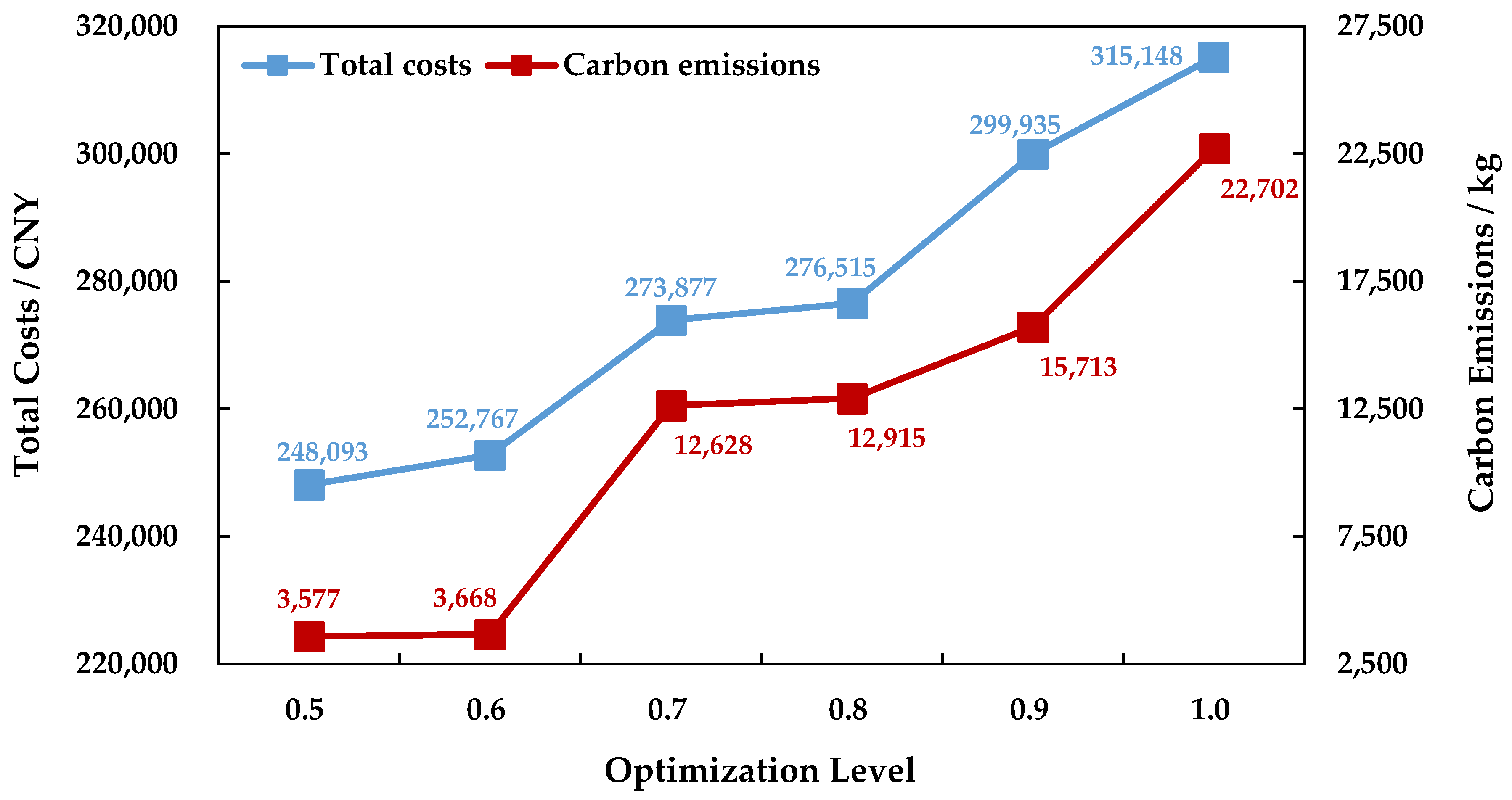
The optimization level $\lambda$ is determined by the receiver according to its attitude towards the RT, and might influence the optimization result. We considered that the receiver prefers a high optimization level that falls in the interval [0.5, 1.0] to ensure reliable transportation. We accordingly increased the optimization level from 0.5 to 1.0 with a step of 0.1 to determine the TCs and CEs of the PIMRs under different optimization levels. The sensitivity of the GIMRPMTWIFCCTR concerning the optimization level is illustrated in Figure 1.

As we can see from Figure 1, with the improvement in the optimization level, the TCs and CEs of the PIMR both increase, which means that addressing the capacity and carbon tax rate uncertainty significantly influences routing optimization. It is clear that enhancing the RT through improving the optimization level worsens both the economic and environmental sustainability of the GIMRPMTWIFCCTR. Based on Figure 1, the receiver can determine a suitable optimization level that satisfies its requirements to balance the objectives of lowering CTs, reducing CEs, and enhancing the RT. The IMO can then make a plan based on the given optimization level and accordingly organize the IMT.

4.2. Feasibility Analysis of Uncertainty Modeling

Currently, the uncertainty of both carbon tax rate and capacity has not been formulated in existing relevant studies. Therefore, it is necessary for us to demonstrate whether considering twofold uncertainty can improve GIMRP optimization. To verify such feasibility, we compare the uncertainty modeling of the GIMRP with deterministic modeling. We thereby built the following three deterministic scenarios. A deterministic model can be established by replacing the interval fuzzy parameters of the model proposed in Section 3 with their deterministic settings. The planned intermodal route in a deterministic scenario can be obtained by solving the deterministic model using the same software and algorithm.

(1)

The receiver holds an optimistic decision-making attitude in the GIMRP. In this case, the minimum carbon tax rate (i.e., $p^{-}$) and the maximum capacities (i.e., ${\eta }_{ijr}^{+}$ and ${\eta }_j^{rs+}$) are used by the IMO to make a plan. The TCs of the PIMR in this deterministic scenario are CNY 214,027. This is identical to the result of the uncertainty modeling when the optimization level is 0, which means that it yields an extremely low reliability in the actual transportation environment where uncertainty exists and results in unreliable transportation;

(2)

The receiver holds a pessimistic decision-making attitude in the GIMRP. In this situation, the maximum carbon tax rate (i.e., $p^{+}$) and the minimum capacities (i.e., ${\eta }_{ijr}^{-}$ and ${\eta }_j^{rs-}$) are used by the IMO to make a plan. The TCs of the PIMR in this deterministic scenario are CNY 315,148, and this is identical to the result of the uncertainty modeling when the optimization level is 1.0;

(3)

The receiver holds a compromised decision-making attitude in the GIMRP. Therefore, the mean values (i.e., ${\displaystyle \frac{p^{-}+p^{+}}{2}}$, ${\displaystyle \frac{{\eta }_{ijr}^{-}+{\eta }_{ijr}^{+}}{2}}$, and ${\displaystyle \frac{{\eta }_j^{rs-}+{\eta }_j^{rs+}}{2}}$) of the upper and lower bounds of the corresponding interval fuzzy parameters are used by the IMO to plan the intermodal route. The TCs of the PIMR in this deterministic scenario are CNY 248,093, and this is the same as the result of the uncertainty modeling when the optimization level is 0.5.

Above all, uncertainty modeling can present a series of optimization-level-sensitive intermodal routes that fully reflect the receiver’s different decision-making attitudes in the GIMRP, and thus significantly improves the flexibility of the problem optimization and helps the IMO to plan the most suitable transportation scheme to match the receiver’s requirements, which might change in the planning stage. Moreover, uncertainty modeling can help to avoid plans that yield a low RT by restricting the optimization level. Consequently, uncertainty modeling is able to improve problem optimization, and should be highlighted in transportation planning studies.

4.3. Feasibility Verification of Mixed Time Window

Currently, there are no studies that employ an MTW in the GIMRP under the uncertainty of both capacity and carbon tax rate. Therefore, there is no existing evidence verifying the feasibility of the MTW under these conditions. With reference to Ge et al. [16], this study compares the MTW with the HTW and STW to show its feasibility.

Under the HTW, the delivery of containers must be accomplished within $[\pi ,{\pi }^{\prime }]$. In this case, the objective of model formulating the GIMRP with a HTW under capacity and carbon tax rate uncertainty is shown in Equation (31), and its constraints are shown in Equations (2)–(7), (14)–(18), (21), (27)–(29), (32), and (33).

$$\min {\displaystyle \sum _{(i,j)\in A}{\displaystyle \sum _{r\in S_{ij}}{c}_{ijr}\cdot q\cdot x_{ijr}}}+{\displaystyle \sum _{j\in N}{\displaystyle \sum _{r\in S_j}{\displaystyle \sum _{s\in S_j}{c}_j^{rs}\cdot q\cdot y_j^{rs}}}}+\xi$$

(31)

$$z\ge \pi$$

(32)

$$z\le {\pi }^{\prime }$$

(33)

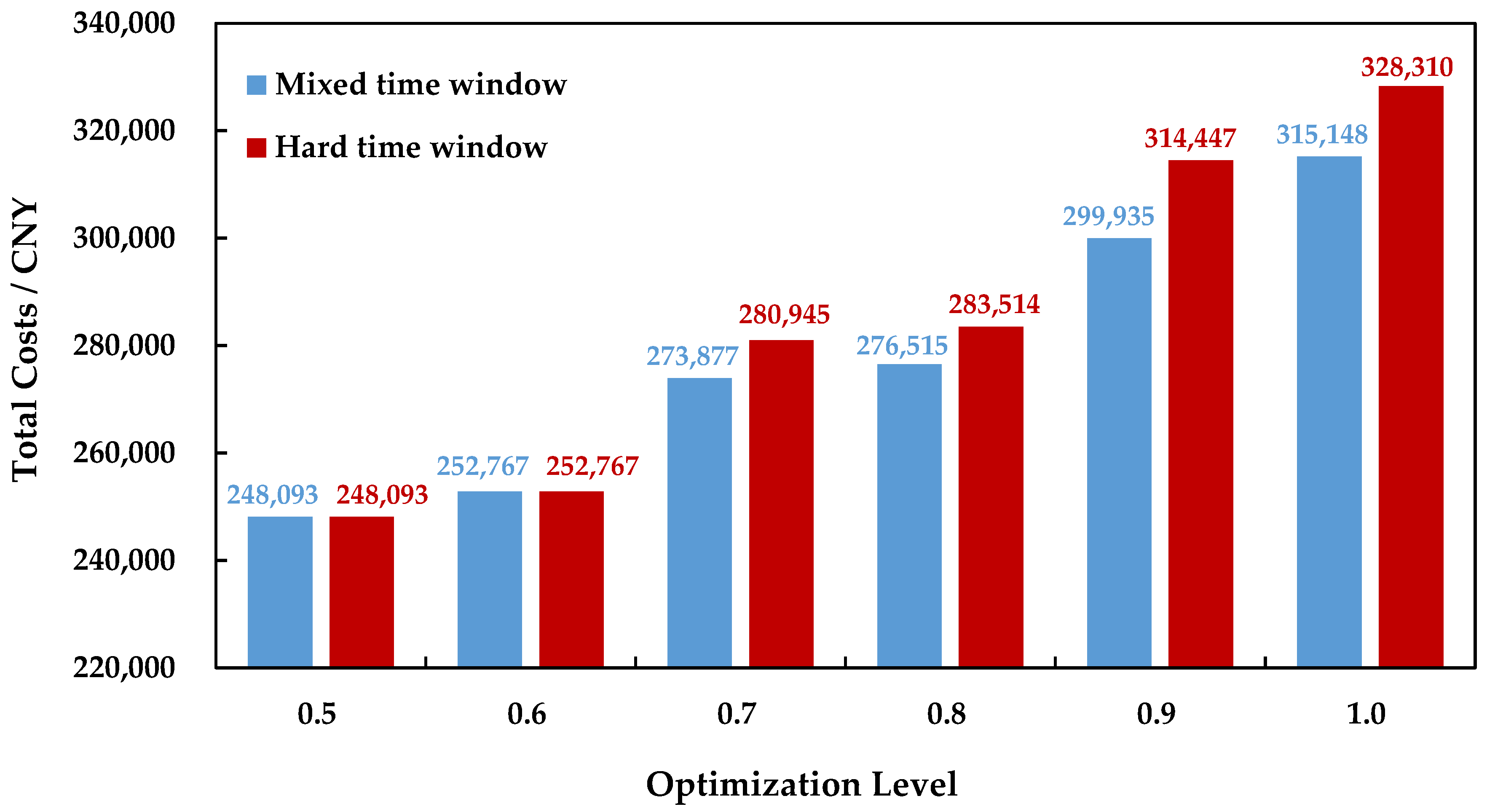
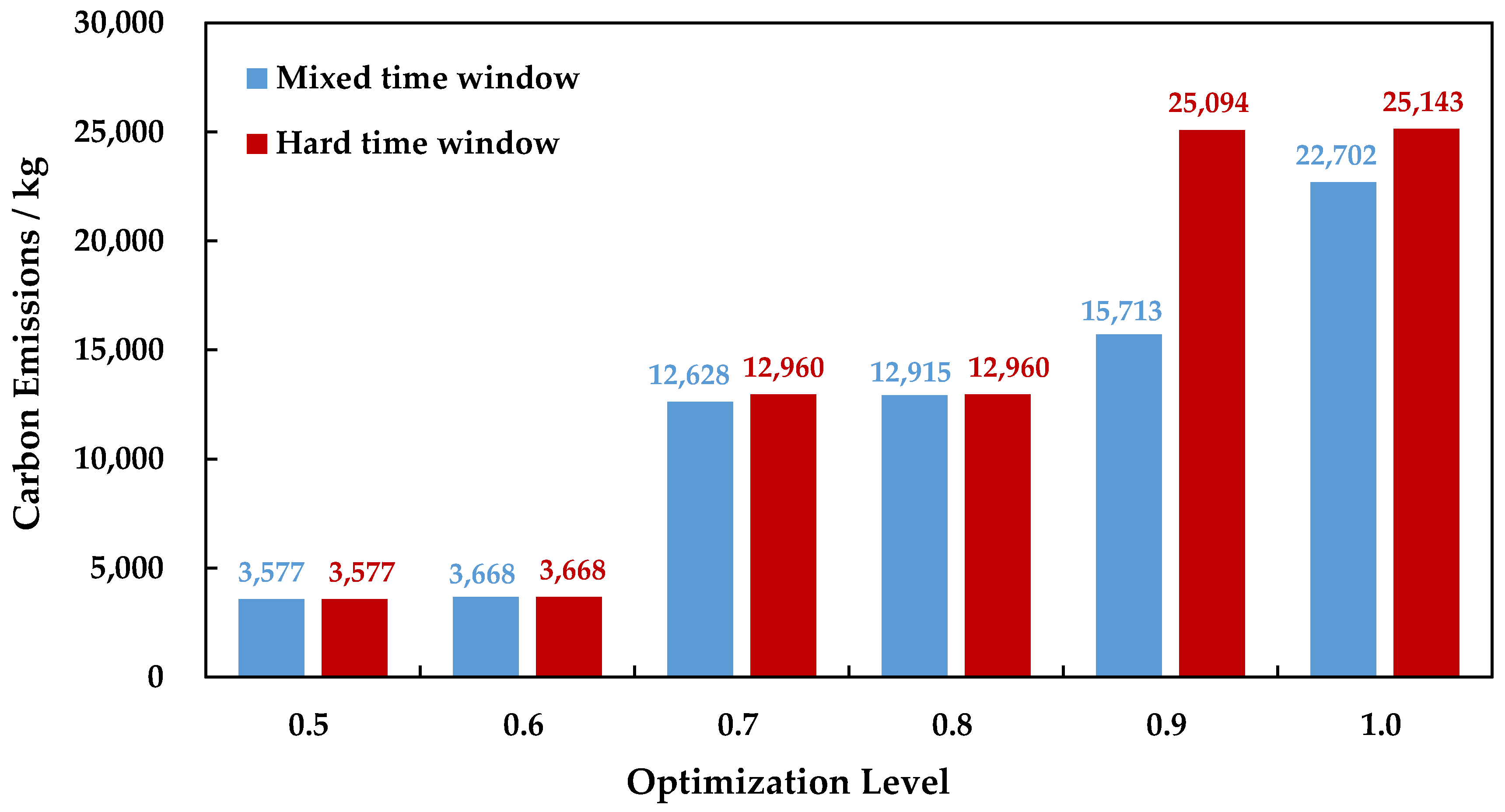
The comparisons between the HTW and MTW under different optimization levels are illustrated in Figure 2 and Figure 3. According to Figure 2 and Figure 3, the two types of time window yield the same results under lower optimization levels of 0.5 and 0.6. However, when the optimization level is improved to satisfy the receiver’s requirement of a higher RT, the use of MTW can reduce both the TCs and CEs of the PIMR when compared to the HTW. Consequently, the MTW is more feasible than the HTW in the GIMRP under capacity and carbon tax rate uncertainty.

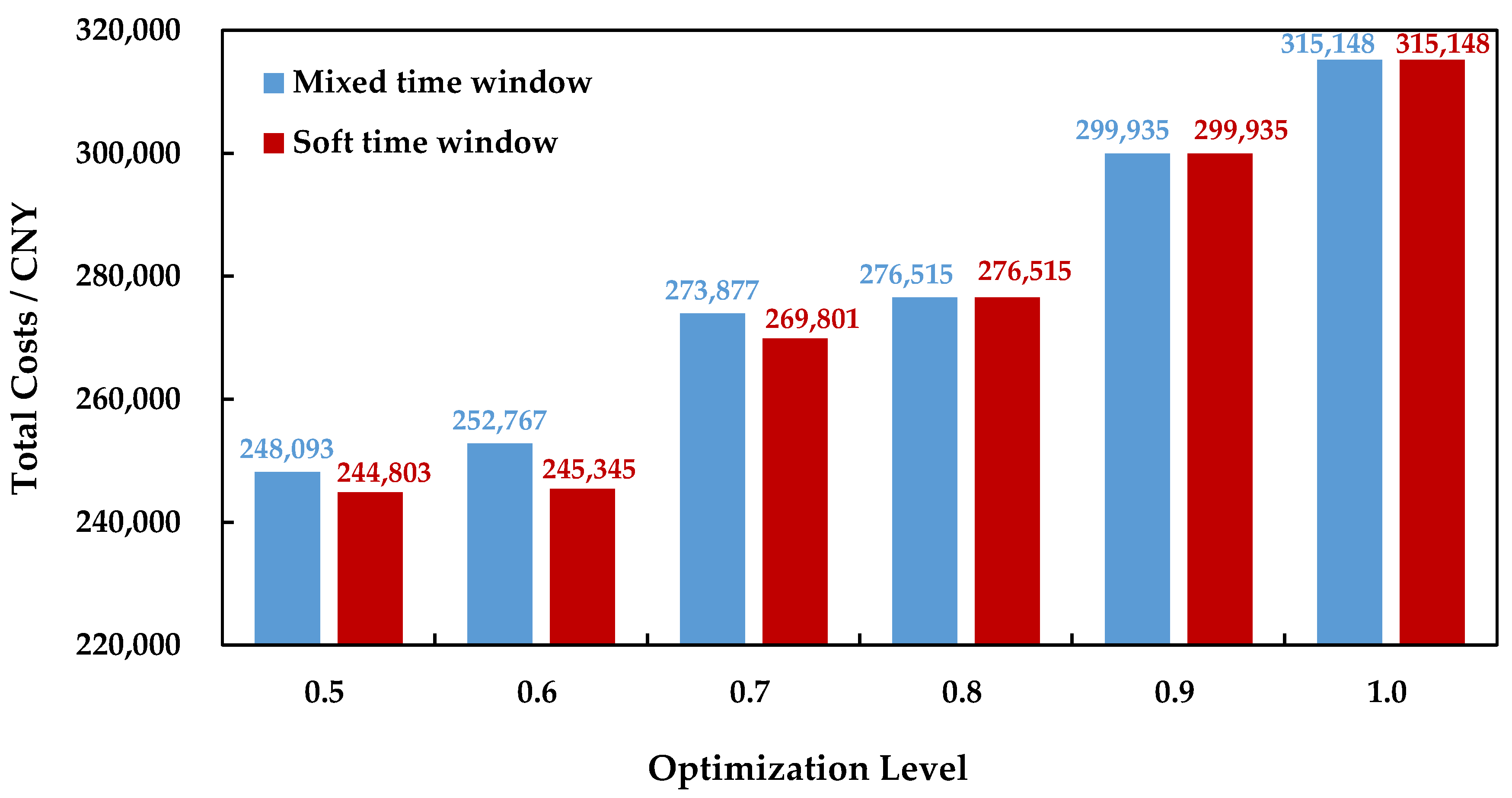
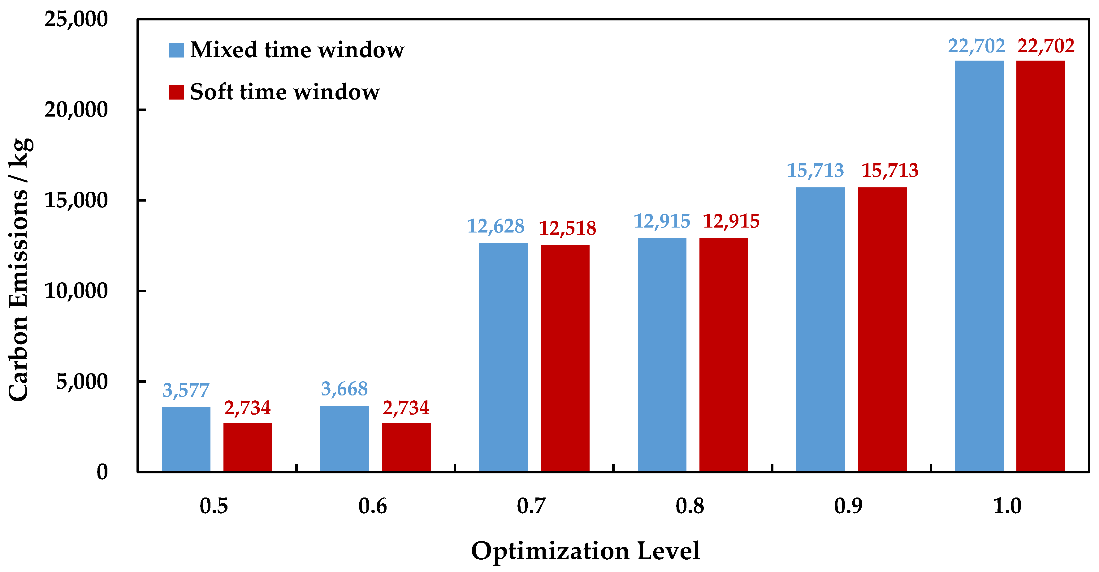
When using the STW, the GIMRP takes Equation (19) as the objective and its constraints cover Equations (2)–(9), (14)–(18), (21), and (27)–(29). The comparisons between the STW and MTW under different optimization levels are illustrated in Figure 4 and Figure 5.

As shown in Figure 4 and Figure 5, when the receiver pays less attention to the RT and determines lower optimization levels of 0.5, 0.6, and 0.7, the STW helps to reduce the TCs and CEs of the PIMR when compared to the MTW. When the receiver demands higher optimization levels to ensure reliable transportation, the two time windows give identical results. 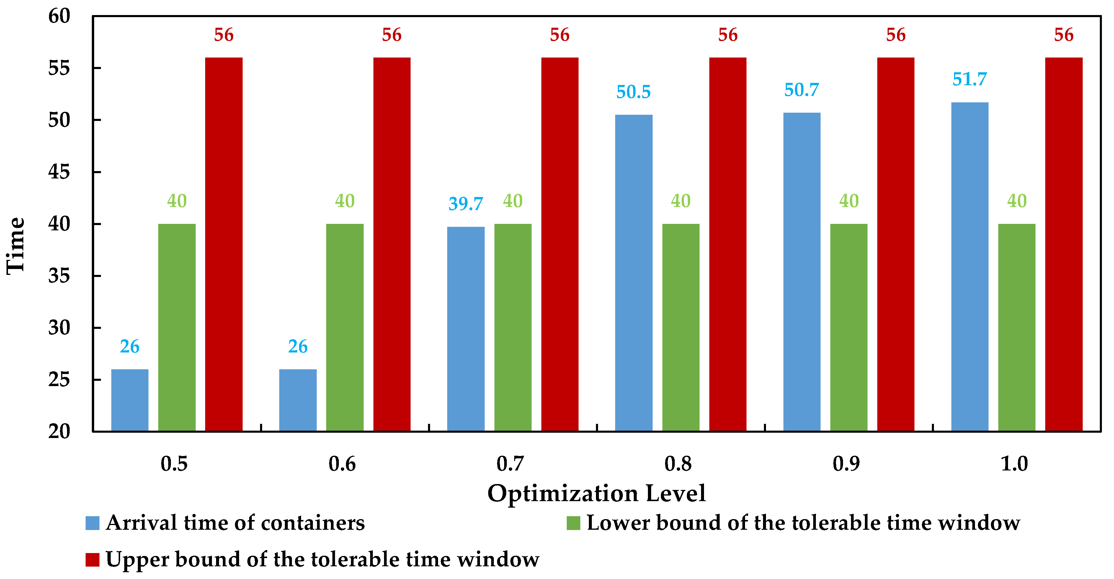Furthermore, we calculate the delivery time of containers under the STW, which is given in Figure 6.

As shown in Figure 6, when the STW obtains better optimization results than the MTW, the delivery times of containers under STW are earlier than 40 (i.e., 16:00 on day 2), which is too early and violates the receiver’s timeliness requirement indicated by the tolerable time window. Consequently, the MTW enables the receiver’s requirements to be satisfied in all the decision-making scenarios. Therefore, the MTW is more feasible than the STW in the GIMRP investigated in this study.

Above all, the HTW could lead to higher TCs and CEs, and the STW could fail to avoid overly early delivery in some decision-making scenarios. However, the MTW is able to avoid these issues. Consequently, we have verified that the MTW is better than the HTW and STW when employed in a GIMRP that considers uncertainty in the capacity and carbon tax rate.

4.4. Feasibility Analysis of Carbon Tax Regulation Under an Uncertain Carbon Tax Rate

To date, there have been no relevant studies showing the feasibility of CTR in the GIMRP under the uncertainty condition addressed in this study. Therefore, it is necessary to analyze the feasibility of CTR in the scenario discussed in this study. With reference to Sun et al. [7,10], the carbon emission minimization method (CEMM) is used as a benchmark to verify whether CTR can effectively reduce the CEs of the PIMR under an uncertain carbon tax rate. Equation (34) shows the objective and Equations (2)–(9), (14)–(18), (27), and (27) show the constraints of the GIMRP model that minimizes CEs.

$$\min {\displaystyle \sum _{(i,j)\in A}{\displaystyle \sum _{r\in S_{ij}}{e}_{ijr}\cdot d_{ijr}\cdot q\cdot x_{ijr}}}+{\displaystyle \sum _{j\in N}{\displaystyle \sum _{r\in S_j}{\displaystyle \sum _{s\in S_j}{e}_j^{rs}\cdot q\cdot y_j^{rs}}}}$$

(34)

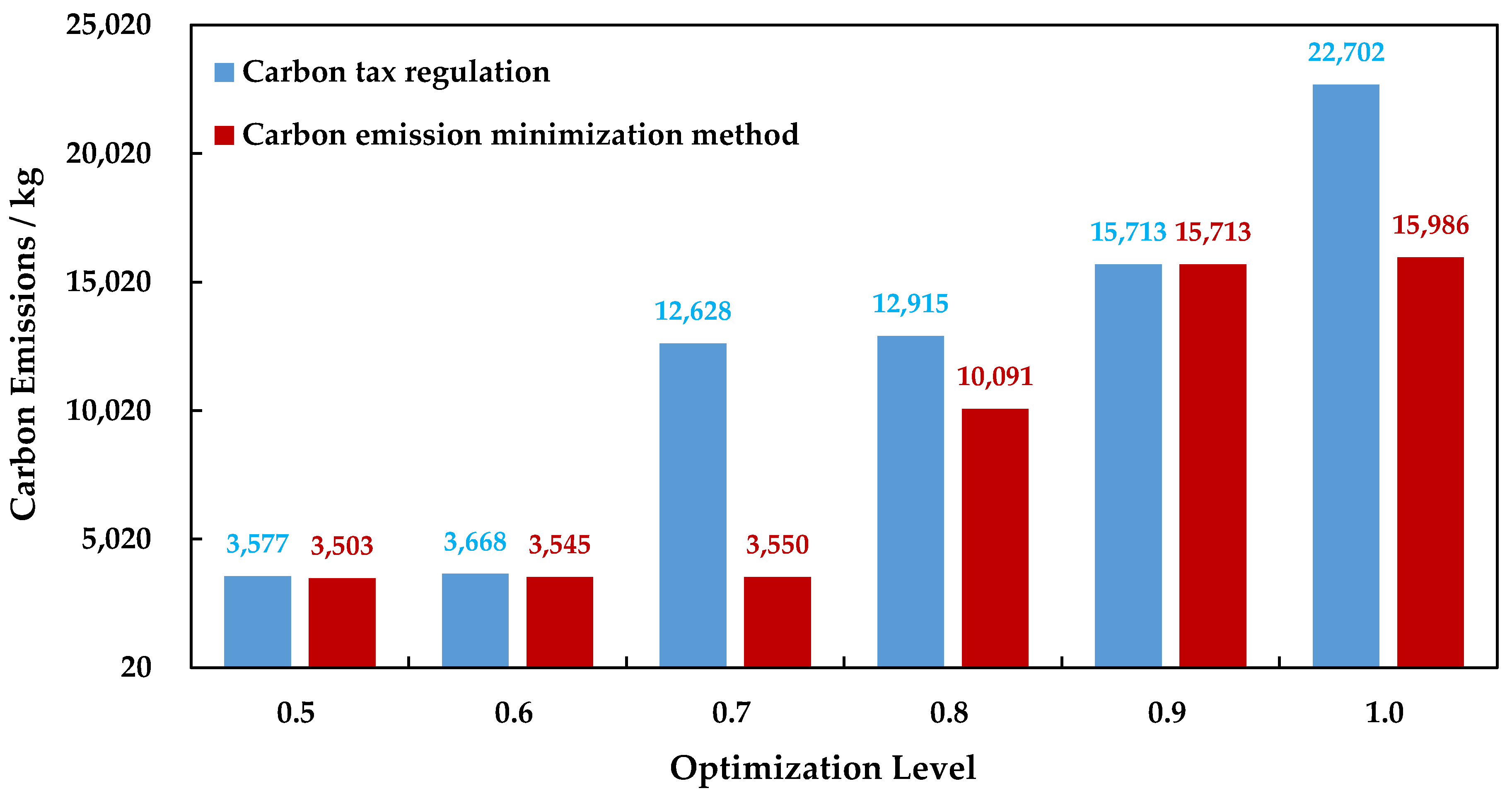
The CEs of the PIMR using CTR and the CEMM under different optimization levels are illustrated in Figure 7. Compared to the CEMM, CTR increases the CEs of the PIMR by an average of 55.2% in all decision-making scenarios, and the root mean square error (RMSE) in the CEs between the two methods is 4725 kg.

As we can see from Figure 7, the gap in the CEs between the two methods is significant when the optimization level is 0.7. Under this condition, CTR leads to CEs that are 3.6 times larger than these of the CEMM. Without this optimization level, the increase in the CEs by CTR in the remaining decision-making scenarios can be reduced to 15.1% from 72.6% when compared to the CEMM, and their RMSE of CEs can be lowered by 31% to 3258 kg. Therefore, CTR shows good performance in reducing CEs when the optimization levels are 0.5, 0.6, 0.8, 0.9, and 1.0. However, its performance under an optimization level of 0.7 is limited.

To summarize, CTR is not always feasible in all decision-making scenarios, which is in line with the conclusion drawn by Sun et al. when considering a deterministic carbon tax rate [7]. When the receiver prefers an optimization level of 0.7, which makes CTR infeasible, a bi-objective optimization (BOO) can be adopted as an alternative to address the green intermodal routing problem [7]. The objectives of the BOO model for the GIMRP are shown in Equations (34) and (35) and Equations (2)–(11), (14)–(18), (27), and (28) are formulated as the constraints.

$$\min {\displaystyle \sum _{(i,j)\in A}{\displaystyle \sum _{r\in S_{ij}}{c}_{ijr}\cdot q\cdot x_{ijr}}}+{\displaystyle \sum _{j\in N}{\displaystyle \sum _{r\in S_j}{\displaystyle \sum _{s\in S_j}{c}_j^{rs}\cdot q\cdot y_j^{rs}}}}+c_{pen}\cdot q\cdot w+{c^{\prime }}_{pen}\cdot q\cdot w\prime$$

(35)

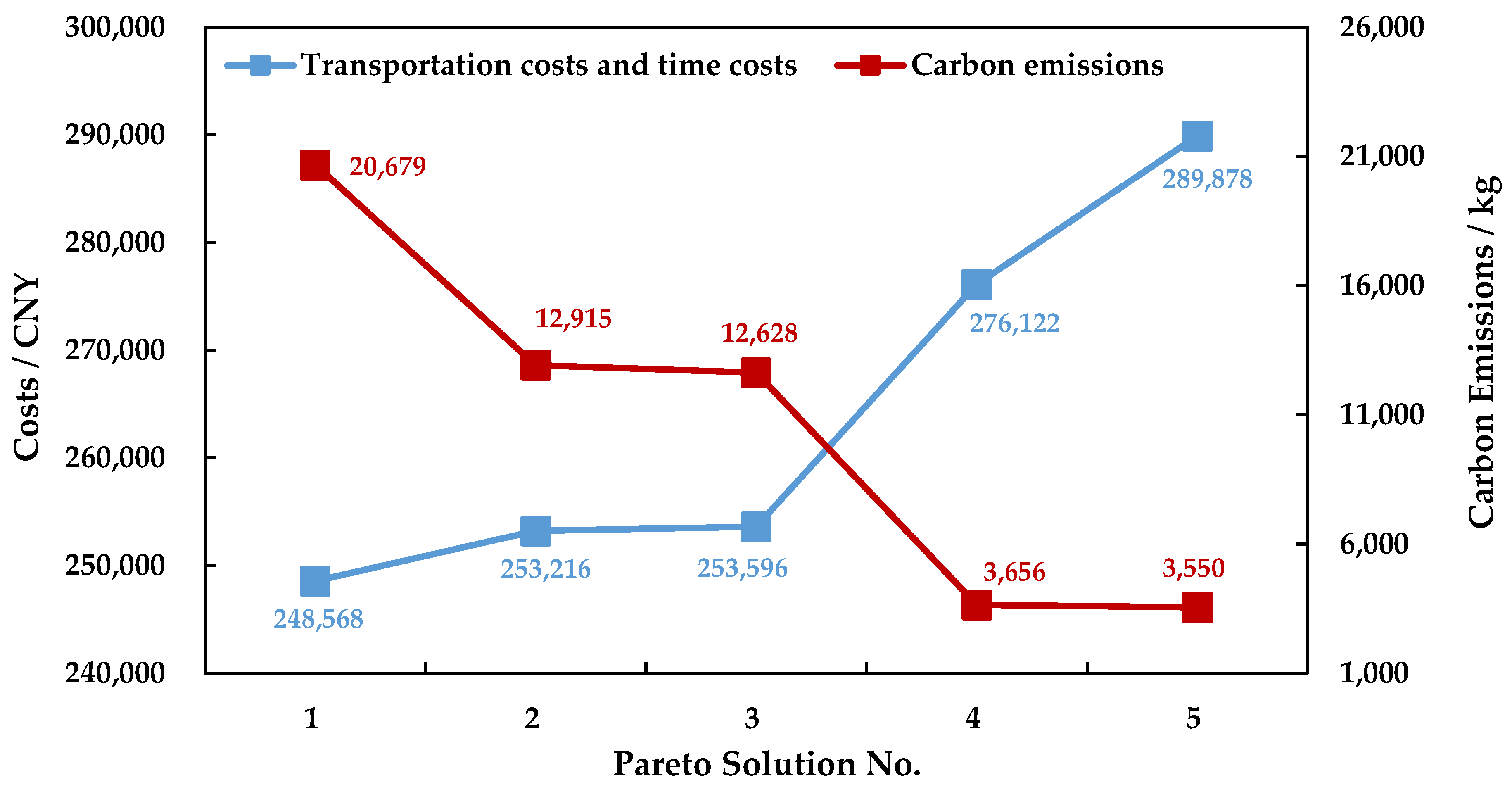
Under the optimization level of 0.7, a weighted sum method is used in this study to obtain the Pareto solutions to the BOO model. The Pareto solutions are listed in Figure 8. Figure 8 indicates that there is a conflict between lowering the sum of the transportation and time costs and reducing the CEs. The improvement in one objective will worsen another one. Therefore, the Pareto solutions can be used to make tradeoffs between the two objectives when CTR is infeasible under the optimization level of 0.7. For example, when increasing the sum of transportation and time costs by 8.9%, Pareto solution 4 can lead to CE reductions of 71% compared with Pareto solution 3. Therefore, Pareto solution 4 is more suitable as the IMT scheme than Pareto solution 3 on the conditions that it satisfies the receiver’s budget and the receiver is also willing to reduce CEs.

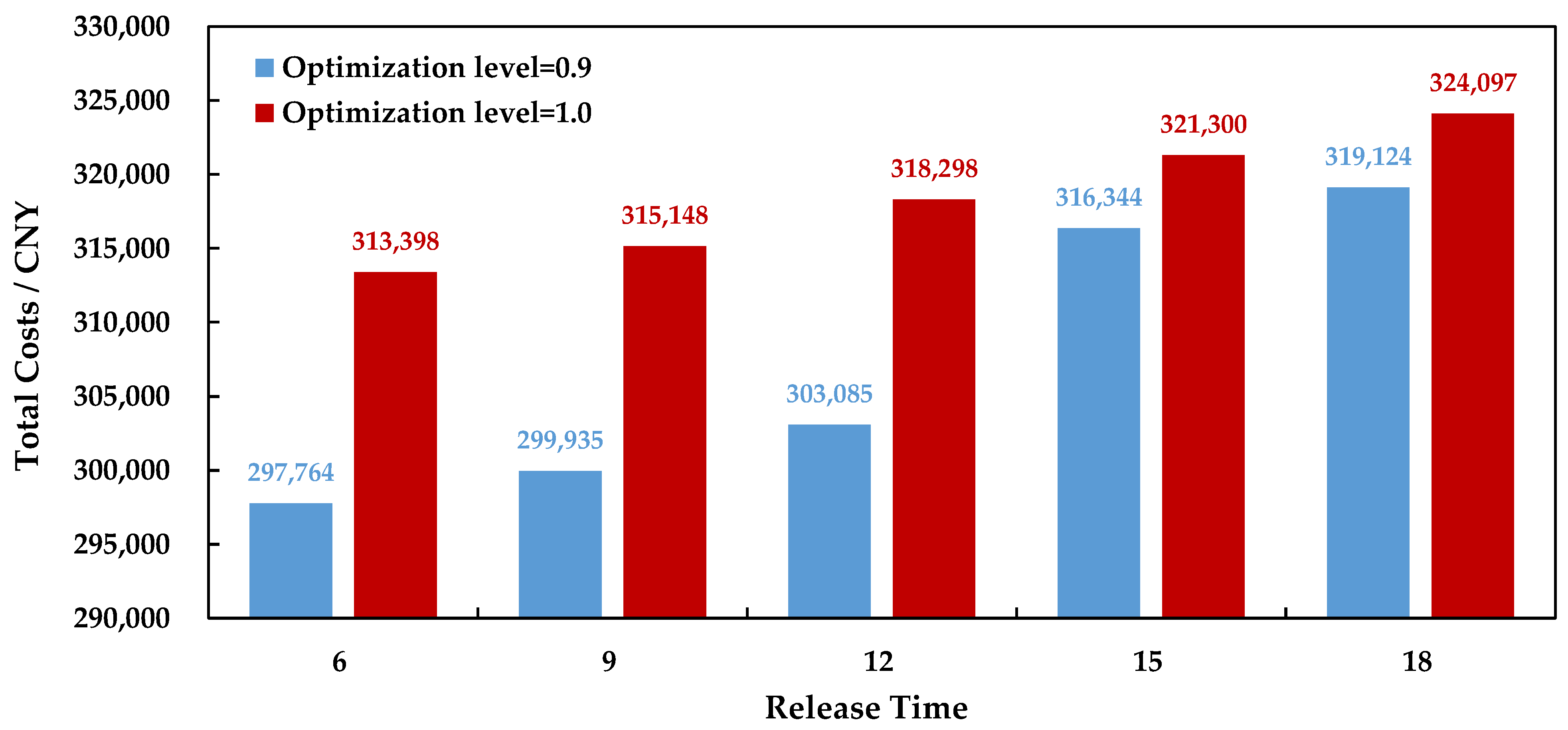
4.5. Influence of the Release Time of the Shipper on Routing Optimization

The MTW of the receiver is predetermined based on the post-transportation processing schedules and is thereby difficult to change flexibly. However, the release time of containers at the origin can be negotiated between the shipper and receiver and is thus adjustable. In this section, we discuss how the release time influences the routing optimization where the receiver prefers a high RT.

In this case, we set the optimization levels as 0.9 and 1.0 and the release times as 6, 9, 12, 15, and 18, to obtain the TCs of the PIMRs under different combinations these parameters. The results are illustrated in Figure 9.

As indicated by Figure 9, the release time of containers influences the GIMRPMTWIFCCTR. Under the condition that the receiver prefers a high RT and accordingly requires a high optimization level, the TCs of the PIMR become lower the earlier the containers are released at the origin. When changing the release time from 18 to 6, the TCs of the PIMR are reduced by 6.7% for the confidence level of 0.9 and 3.3% for the confidence level of 1.0.

Therefore, an earlier container release time helps the receiver to reduce the TCs of the PIMR with a high RT to a certain degree. In this case, the shipper and receiver should negotiate effectively to enable the shipper to release the containers of the transportation order quickly, allowing a PIMR with lower costs and higher RT to be provided to the receiver by the IMO.

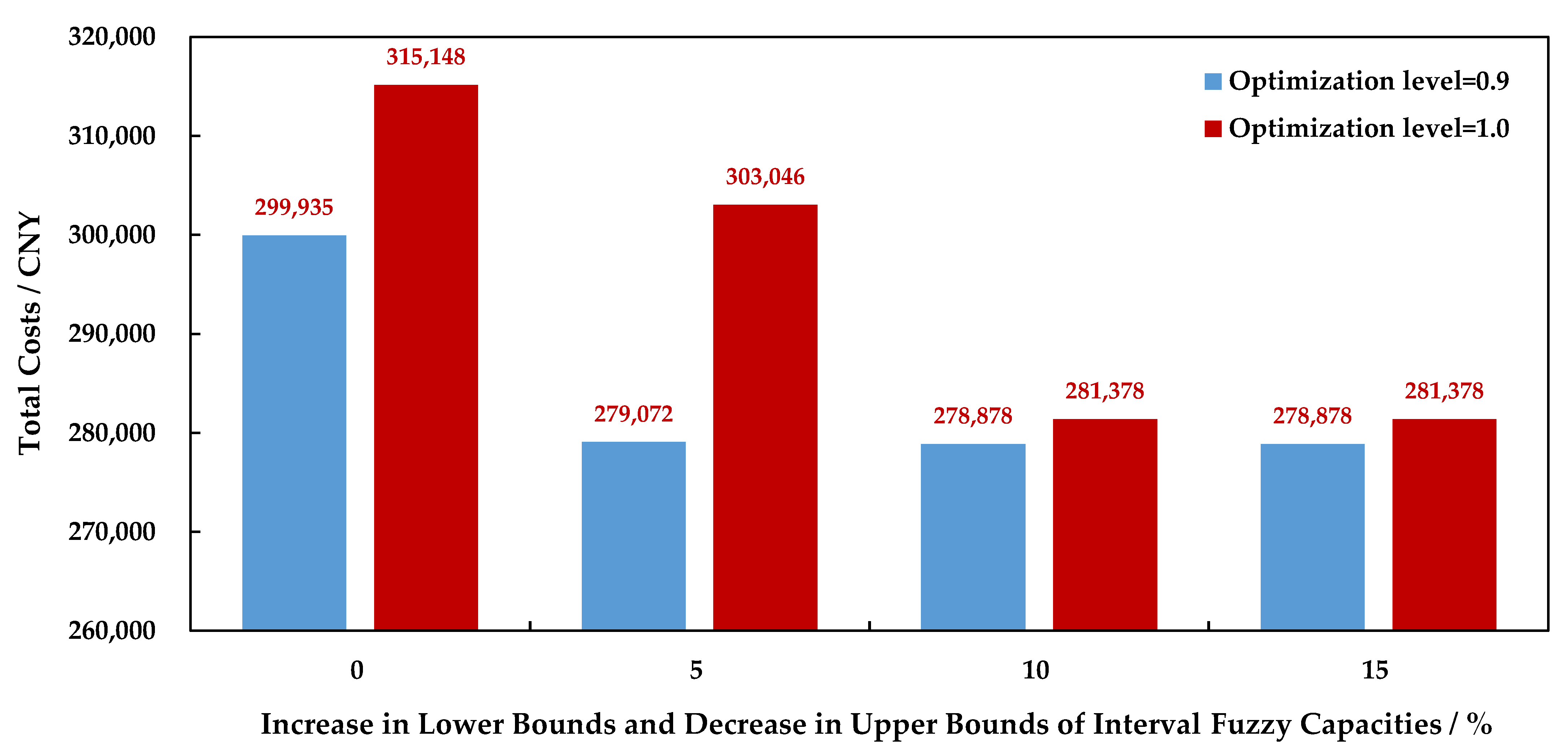
4.6. Influence of the Stability of the Interval Fuzzy Capacity on Routing Optimization

The range of an interval fuzzy number can reflect its stability and is determined by its upper and lower bounds. The stability of the interval fuzzy number is enhanced when the two bounds are closer to each other. In this section, we fix the interval fuzzy carbon tax rate, since it is determined by the practical market and cannot be changed by the receiver or the IMO. Therefore, we only discuss the influence of the stability of the interval fuzzy capacity on the routing optimization.

We still assume that the receiver prefers a high RT and set the optimization levels as 0.9 and 1.0. We increase the lower bounds and decrease the upper bounds of the interval fuzzy capacities of the intermodal network from 0% to 15% in steps of 5%, and provide the routing optimization under different interval fuzzy capacity ranges, as illustrated in Figure 10.

As we can see from Figure 10, improving the stability of the interval fuzzy capacity by narrowing its range from the lower bound to the upper bound reduces the TCs of the PIMR that yields a high RT to a certain degree. When the stability of the interval fuzzy capacity is improved through separately increasing the lower bound and decreasing the upper bound by 15%, the TCs of the PIMR are reduced by 7% for the confidence level of 0.9 and 10.7% for the confidence level of 1.0.

Therefore, when building a water–rail–road intermodal network, besides considering the capacity sufficiency, the IMO should consider the stability of the capacity. Transportation modes with more stable capacities should be used to carry out transit processes, and transfer nodes with more stable capacities should be adopted to realize the transfer process between different transportation modes.

5. Conclusions

In this study, we explore a GIMRPMTWIFCCTR, in which the economic, environmental, and reliability objectives are comprehensively considered. Based on the use of IFNs to model uncertainty, we propose an IFLOM to address the specific routing problem and further present its crisp reformulation, in which the optimization level is introduced to indicate the receiver’s attitude towards the RT. The following conclusions are drawn:

(1)

Modeling the capacity and carbon tax rate uncertainty in the GIMRP and introducing the optimization level in the crisp processing of the IFLOM enable the different decision-making attitudes of receivers to be fully measured, improve the flexibility of the routing decision-making, and avoid unreliable transportation;

(2)

Achieving a reliable intermodal route through improving the optimization level worsens both the economic and environmental sustainability of the route. Therefore, the receiver must select a suitable optimization level to balance these objectives based on their attitude towards the RT, their budget, and their willingness towards CE reduction;

(3)

An MTW is more feasible than the HTW and STW in ensuring the timeliness of GIMRP. Therefore, in the routing stage, the receiver should accurately determine their tolerable and expected time windows to establish an MTW that matches the post-transportation processing of good;

(4)

Under an uncertain carbon tax rate, CTR is not feasible in all decision-making scenarios. When CTR is infeasible, the BOO can be used by the IMO and receiver to balance the economic and low-carbon objectives of the GIMRP;

(5)

The release time of containers influences the GIMRPMTWIFCCTR to a certain degree. An earlier release time can help the receiver to reduce the TCs of the PIMR that maintains a high RT, which relies on effective negotiation between the shipper and the receiver.

(6)

The stability of the interval fuzzy capacity also influences the GIMRPMTWIFCCTR to a certain degree. The IMO should improve the capacity stability of the intermodal network to provide the receiver with a transportation service that yields both lower TCs and higher RT.