Abstract
Innovation-driven development is the main driving strategy for promoting high-quality economic development. Technological innovation is the core of innovation-driven development. Financial innovation is an important aspect of promoting financial development. As such, the coupling and coordination of the technological innovation and financial development in developing countries, such as China, is an important issue. The topic has been extensively studied over the last decade in the context of China, and a dominating method has emerged on how to model the technological innovation subsystem and the financial development subsystem, and how to quantitatively determine the degree of coupling and coordination of the two subsystems. A variety of predictors have been proposed to model each subsystem. The coupling degree and the coordination degree are then calculated, and then they are used to analyze the current development status for potential issues. However, we make an effort to validate the calculated degree of coupling and coordination before the results are used for the analysis.Without validation, the outcomes of the analysis not only might not be useful but also could lead to inappropriate governmental policies. That said, it is tremendously challenging to validate the results due to the lack of the ground truth. The goal of this study is to work towards objectively determining the reliability of the degree of coupling and coordination from an engineering perspective. Specifically, we accomplish this task by evaluating the regression performance and projection performance. We demonstrate that the use of a carefully crafted set of predictors for each subsystem is the foundation for deriving the reliable coordination degree of the two subsystems.
1. Introduction
Since early 1980s, China’s economy has achieved rapid growth and has become the world’s second largest economy. The economic structure in China has been continuously shifting from the original extension-driven growth predominantly driven by low-cost labor, to endogenous growth driven by innovation. In order to accelerate the construction of the national innovation system, the Chinese government has enacted policies that encourage innovation-driven development. Financial innovation has become a key driving force for financial development in recent years.
From the perspective of system theory [1], technological innovation can be regarded as a subsystem, and financial development can also be regarded as a subsystem. If there is a benign coupling and coordinated interaction between the two systems of technological innovation and financial development, and they promote each other and develop together, they create a win–win situation. However, in practice, the two subsystems may suffer from a number of issues, such as insufficient interaction, mismatch between supply and demand, and uncoordinated development. Therefore, it is of great significance to examine the coupling and coordinated development of the two systems, promote the combination of technology and finance, and achieve coordinated development, in order to achieve stable economic development. As such, the relationship between technological innovation and financial development has been extensively studied over the last decade [2,3,4,5,6,7,8,9], and a dominating method has emerged on how to model the technological innovation subsystem and the financial development subsystem, and how to quantitatively determine the degrees of coupling and coordination of the two subsystems. A variety of predictors have been proposed to model each subsystem. The degree of coupling and the degree of coordination are then calculated, and then they are used to analyze the current development status for potential issues.
However, we make an effort to validate the calculated degrees of coupling and coordination before the results are used for the analysis.Without validation, the outcomes of the analysis not only might not be useful but also could lead to inappropriate governmental policies. That said, it is tremendously challenging to validate the results due to the lack of the ground truth. The goal of this study is to work towards objectively determining the reliability of the degree of coupling and coordination from an engineering perspective. Specifically, we accomplish this task by evaluating the regression performance and projection performance. We demonstrate that the use of a carefully crafted set of predictors for each subsystem is the foundation for deriving a reliable coordination degree of the two subsystems.
The remainder of this article is organized as follows. Section 2 outlines the related work and highlights the differences between our study and the related studies. Section 3 describes the mainstream theory on modeling the coupling and coordination of two correlated subsystems. In this section, we also elaborate the set of 12 predictors for the technological innovation subsystem, and the set of 12 predictors for the financial development subsystem that we propose for the current study. Section 4 reports the data source that we use to calculate the predictors. Section 5 elaborates the details of data processing using the model we describe in Section 3, and the results, including the comprehensive evaluation index for each of the two subsystems, the coupling degree, and the coordination degree. To demonstrate the importance of using the right set for each subsystem, all calculations are performed, and all results are presented side by side with the predictors that we introduce and the predictors proposed in the first significant study on the coupling and coordination of the two subsystems [3]. This section also presents the objective evaluation on the quality of the calculated degrees of coupling and coordination. Section 6 reports an in-depth discussion on several aspects of our study, including three alternative configurations (using a reduced predictor set, using alternative imputation methods, and using an alternative weighting method), and statistical comparison of the outcomes derived from different configurations, including using our dataset and the reference dataset. Section 7 concludes this article and identifies the limitations of the current study. Furthermore, four appendices are included to report detailed information that might not be critical for understanding our study, but could be of interest to readers, including the predictors introduced in related studies, the coupling degree matrices, and the coordination degree matrices.
2. Related Work
Our study falls under the umbrella of the general system theory [1], where a system is modeled as consisting of cohesive groups of interrelated and interdependent components (or subsystems). Naturally, the coupling and coordination of the subsystems would be of interest in understanding the system. One of the first publications on the coupling of two systems in the field of socio-economy is [10] (published in 1947), where a quantitative model was proposed to calculate the degree of coupling between two correlated systems, particularly focusing on the markets with production lags. The concept of loosely coupled systems and the necessity of evaluating the strength of loosely coupled systems in the context of educational organizations was proposed in [11].
2.1. Coupling and Coordination Studies
The coupling and coordination between a variety of correlated subsystems are seen in the field of finance and economic. These studies have considered the coupling and coordination between environmental pollution and economic development [12], human capital and economic growth [13,14], tourism industry and regional economic development [15], resource endowment, ccological environment, and economic development [16], digital economy and green finance [17], intellectual property and economy [18], urbanization and ecological environment [19]. It is also interesting to note that in [20], the coupling and coordination calculation is used to determine predictors that indicate obstacles in economic development by comparing the coupling and coordination between different predictors (a total of 10 subsystems are considered based on first-level predictors).
Several studies focused on proposing coupling mechanisms between technological innovation and financial development. In [21], the important of the coupling and coordination between technological innovation and financial development is recognized and advocated appropriate policies to facilitate the coupling and coordination. In [22], three levels of mechanisms are proposed to enhance the coupling and coordination of technological innovation and financial development: (1) financing of science and technology industrial parks; (2) setting up technology financial institutions; and (3) subsidizing market-oriented operation. In [23], the coupling mechanisms proposed include the setup of independent regulatory Institutions, encourage the integration of research and development in enterprises, provide support for big data and wide-band connectivity, and enact suitable governmental policies. In [24], a dynamic model to facilitate the coupling and coordination of the two subsystems is proposed. The model consists four feedback loops with similar steps: financial investment on research institutions, which would produce more papers and patents, then in turns, the intellectual properties could lead to new products and the growth of the local economy. The improved economy would generate more taxes, which makes it possible for the local government to invest more.
Several studies [2,3,4,5,6,7,8,9] adopted the same set of models and formula for calculating the degree of coupling and coordination between technological innovation and financial development. Some studies [25] described the formula used to calculate the comprehensive evaluation index, the coupling degree, and the coupling and coordination degree with citations but did not explicitly provide the formulas. From the context, it appears that the formulas are likely the same.
In [2], a total of six predictors for both the technological innovation and financial development are used to model the coupling between new industry and traditional industry, instead of treating technological innovation and financial development as two subsystems.
In [3], the focus is on applying the set of formulas to discover the economical development in China based on the 2002–2012 data, while in [4], the focus is on examining the impact on economic efficiency without presenting the detailed outcomes of the degree of coupling and coordination. In [3], two categories of seven predictors are used to model the technological innovation subsystem, and three categories of seven predictors are used to model the financial development subsystem. The proposed model is applied to data collected in China between 2002 and 2012.
In [5], two categories of four predictors are used for the technological innovation subsystem, and three categories of three predictors (one per category) are used for the financial development subsystem. The model is applied to the 2008–2013 data.
In [26], four predictors for the technological innovation subsystem are introduced (no category is created), and three predictors for the financial development subsystem (no category is created). The way the coupling degree C is calculated is non-mainstream. The range for C ranges between −1 and 1 instead of between 0 and 1. Furthermore, the model assumes that the comprehensive index for each subsystem would significantly change over the period of time of interest.
In [6], the model is applied to four regions around the Yangtze river using the 2005–2016 data. For the technological innovation subsystem, three categories of eight predictors are used. For the financial development subsystem, also three categories of eight predictors are used.
In [27], the coupling and coordination between technological innovation and industrial structure optimization, as well as the coupling and coordination financial innovation and industrial structure optimization, are studied. The formulas used are not explicitly provided but are presumably similar to those of [3,4,28]. For the technological innovation subsystem, three categories of eight predictors are used. For the financial development subsystem, two categories of nine predictors are used. This study examines the China 2013–2017 data.
In [8], the coupling and coordination of three subsystems instead of two are studied, including culture, technological innovation, and financial development. For the technological innovation subsystem, five predictors of three categories are used. For the financial development subsystem, also five predictors of three categories are used. This study uses the China 2005–2016 data.
In [9], the coupling and coordination between technological innovation, green finance, and industrial policies are studied. Seven predictors of two categories are used to model the technological innovation subsystem. This study uses the China 2008–2015 data.
In [25], 10 predictors for three categories of technological innovation, and 12 predictors for three categories of financial development are used to study the coupling and coordination between different geographical regions instead of those of the two subsystems using China 2006–2016 data.
In [29], the relationship between finance policy and the innovation performance from small-to-medium high-tech businesses is studied. The focus of this study is quite different from (i.e., much narrower scope than) other studies that aim to investigate the correlation between financial development and technological innovation in general. This study uses five predictors for finance policy, and four predictors for the innovation performance. The model used to compute the coupling and coordination degree is slightly different from that adopted in [3,4].
2.2. Coupling and Coordination Modeling
To our best knowledge, the first modern theory on system coupling and coordination in the field of socio-economy is attributed to [30]. In later studies, the theory is refined and extended in a large array of studies [3,12,15]. The actual model is presented in Section 3.
The coupling and coordination requires the calculation of a comprehensive index for each subsystem. Various methods have been proposed. In [14], a genetic algorithm is used to estimate the weights. In [31], principal component analysis is used to determine the weights. In [32], in addition to entropy-based weighting, another method called Criteria Importance Through Intercriteria Correlation (CRITIC) [33] is also used to calculate the weights. CRITIC measures the weight of an indicator by evaluating its volatility and conflict. The standard deviation and correlation coefficient are employed to describe volatility and conflict, respectively. Furthermore, machine learning has also been used to predict the economic development level [34], where the ARIMA time series model, LSTM model, XGBoost model, and a hybrid ARIMA-LSTM-XGBoost model based on them are used. Entropy-based weighting appears to be the most popular method by far [35,36,37,38,39].
2.3. Comparison with Related Studies
The coupling and coordination between technological innovation and financial development, which is the focus of the current study, has been extensively studied previously as we have elaborated above. Furthermore, we also choose to use the dominating model for coupling and coordination. Despite the similarity to existing studies, we make a number of research contributions:
- We use a more comprehensive set of predictors to describe each subsystem than those in existing studies. In Table 1, we summarize the predictors used for related studies and ours. In Section, we demonstrate that by using a comprehensive set of predictors, the predictability and consistency of the coupling and coordination degree are stronger than previous studies.
 Table 1. Comparison of the number of predictors used for the technological innovation subsystem and the financial development subsystem.
 - We perform pre-processing of the data, and use regression to fill the missing data. Although this step is essential in machine learning-based studies, it has not been used in the competing studies to our knowledge. By filling the missing data, we are able to investigate the coupling and coordination degree for a wider range of durations.
- We perform regression-based prediction of future trend on the coupling and coordination degree. Again, this is not reported in competing studies. The reliable prediction of future trend is instrumental to enacting optimal government policies for financial development. A side benefit of doing this is that the quality of the selected predictors can be indirectly assessed by the errors of the regression. The rationale is that if the predictors can truly reflect the development stage of the subsystem, and there is no drastic change of governmental policies, the development of the subsystem would change gradually and easily fit into a regression model.
3. Coupling and Coordination Modeling
We adopt the mainstream coupling and coordination modeling in the field of socio-economy [3,12,15,30]. In this section, we introduce the specific predictors for the technological innovation subsystem and those for the financial development subsystem, the method to calculate the comprehensive evaluation index of each subsystem based on the predictors, the method to calculate the degree of coupling between the two subsystems, and the coordination degree of the two subsystems.
3.1. Predictors
A predictor is a metric that can capture a specific aspect of the subsystem. As we will demonstrate in this paper, the selection of appropriate predictors is essential to establishing robust comprehensive evaluation index, which will ultimately impact the coupling and coordination degree for the two subsystems. The construction of predictors for the technological innovation system focuses on the facts that reflect innovation efficiency [40,41]. The predictors for the financial development are based on the theory of financial structure [42], and the integration of quantitative finance and qualitative finance [43]. Ideally, we want to have a full set of predictors that could reflect all aspects of the subsystem. Unfortunately, that is not always possible, e.g., due to the limited public data. As such, we decide to use 12 predictors (in 3 categories) for each subsystem as described in Table 2.
Table 2.
Categories and predictors used for the two subsystems in our model.
3.2. Comprehensive Evaluation Index
The comprehensive evaluation index U quantifies how well the subsystem is developed based on the setup predictors. More specifically, U is defined by Equation (1):
where () is the i-th normalized predictor for the subsystem, is the weight for predictor , and n is the total number of predictors for the subsystem. As such, U is in the range of 0 and 1, with 0 being the worst and 1 being the best. A key step is to estimate the weight for each predictor. The most dominating method is the entropy weighting method [44]. The first step in calculating the weight for each predictor is to normalize the data across all the years in the dataset. Several normalization methods could be used. In the context of our study, the min-max normalization is used, where each data point is normalized into the range of [0, 1] as defined in Equation (2):
where is the i-th value for the j-th predictor, is the corresponding normalized value, and is the vector for the j-th predictor.
The second step is to calculate the entropy for each predictor according to Equation (3):
where is a constant to scale to the range of [0, 1], m is the number of values for each predictor, and is the entropy of the j-th predictor.
The third step is to calculate the degree of diversification calculated via Equation (4):
Finally, the weight for each predictor is calculated via Equation (5):
It is worth noting that the weight calculation requires the use of the entire dataset for all predictors in the subsystem. Predictors that have higher variability would have low entropy and therefore higher weight. On the other hand, predictors that have less variability would have high entropy and therefore lower weight. The structure of the comprehensive evaluation index and the overall steps in calculating the index are illustrated in Figure 1.
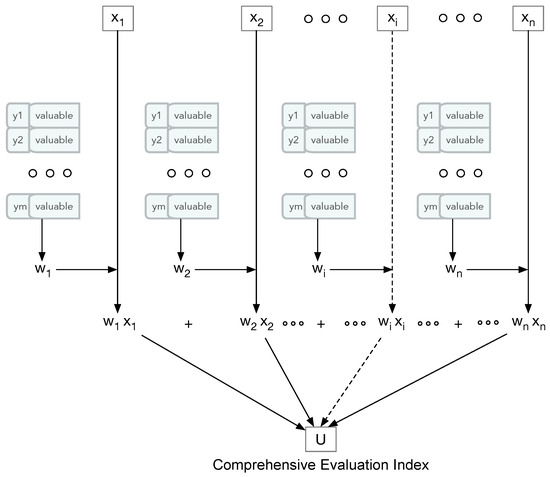
Figure 1.
The structure of the comprehensive evaluation index and the overall steps in calculating the index.
3.3. Coupling Degree
The coupling degree C between two subsystems 1 and 2 quantifies how well the development level of the two subsystems are synchronized with each other. When both subsystems have the same U value, then C would be 1. C is first defined in [30] by Equation (6):
3.4. Coordination Degree
The coordination degree focuses on the subtle relationship between the two subsystems in that the two subsystems should not only be synchronized in their development but also have a symbiotic relationship that makes each other better. D is defined in [30] by Equation (8):
where T is the combined evaluation index for and , and it is defined as , and . If system 1 and system 2 are of equal importance, which is the case of our current study, . As can be seen, unlike C, only when both and are 1 would D be 1. If both and are at a low level of development, D would be close to 0 as well.
4. Data Source
The data for the scientific and technological innovation evaluation index system come from the “China Statistical Yearbook” [45] and the “China Science and Technology Statistical Yearbook” [46]; the data of the financial development evaluation index system come from the “China Finance Yearbook” [47], “China Statistical Yearbook” [45], and “China Regional Financial Operation Report” [48]. The data corresponding to each indicator are processed using the range standardization method, and the four decimal places are uniformly taken, and all the data that are 0 after standardization are replaced with 0.0001 to facilitate logarithmic calculation. The data collected span 2002–2023 and 30 provinces (including autonomous regions and municipalities) in China.
5. Data Processing and Results
To demonstrate our research contribution, it is necessary to compare some of the previous studies that used a different set of predictors. We choose to compare with the first study that adopted the same approach [3], which has 7 predictors for each subsystem. Hence, in each of the following subsections, we present the findings of each dataset side by side. The original study [3] only includes data between years 2002 and 2012. To facilitate direct comparison, we extend the data to 2002–2023 based on the data source.
More precisely, our dataset O consists of the data for all 30 regions between years 2002 and 2023 for each predictor. Recall that we have 12 predictors (, , , , , , , , , , and ) for the technological innovation subsystem, and 12 predictors (, , , , , , , , , , and ) for the financial development subsystem.
The reference dataset R consists of the data for all 30 regions between years 2002 and 2023 for each predictor. There are seven predictors (, , , , , , and ) for the technological innovation subsystem. There are also seven predictors (, , , , , , and ) for the financial development subsystem.
The compiled datasets O and R are saved as two separate Excel sheets. All data pre-processing and processing are carried out using the Python 3.9 programming language on an iMac computer with 64 GB memory. The datasets and all the Python scripts are made available as a GitHub project (https://github.com/wenbingcsu/ccd).
5.1. Data Pre-Processing
Data pre-processing involves two steps: (1) outliner detection, and (2) fill the missing data. For outlier detection, we consider two statistical methods, where one is the z-score method, and the other is the Interquartile Range (IQR) method. The outlier detection gives us an idea of the quality of the data. In the z-score method, a z-score is calculated for each data value based on how many standard deviations it is from the mean. If the z-score for a data item is greater than 3, then it is considered an outlier. The IQR method determines the outliers based on the spread of the middle 50% of the data, and the outliers are values outside of a range bounded by , and , where is the first quantile value, is the third quantile value, and is the difference between and . It is apparent that the method would label more data items as outliners than the z-score method. We perform outlier detection for each predictor for each year of data that are available. Unlike developed countries, regions within China differ significantly in their financial and technological development levels. As such, even if some data items are identified as outliers statistically, they might not be real outliers due to measurement errors. As such, we choose not to replace the values of the outliers for the sake of authenticity of the study.
We log the number of outliers and produce plots for each predictor detected by both outlier detection methods. The maximum number of outliers is 1 in each year of data (among the 30 regions) based on the z-score method, while the number of outliers ranges between 0 and 5 based on the IQR method. Because we choose to use 12 predictors for each subsystem, there are a total of 48 plots for our dataset O. Readers who are interested in viewing these plots may generate these plots via an our source code. Here we only show in Figure 2 two plots for the predictor , one on the number of outliers based on the z-score method, and the other based on the IQR method.
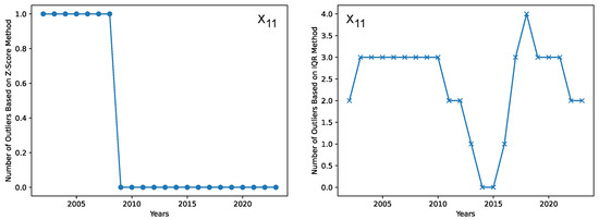
Figure 2.
The number of outliers determined by the z-score method (left), and those by the IQR method (right), both for predictor .
As much as we all would like to have access to all the data, it is inevitable that some data points are not available or invalid. In Table 3, we report the missing data status for each predictor in our dataset O. In Table 4, we report the missing data status for the predictors in the reference dataset R. The detailed definitions of the predictors in the reference dataset R are provided in Appendix A as part of Table A1 and Table A2.
Table 3.
Missing data status in our dataset O.
Table 4.
Missing data status in the reference dataset R.
We decide to use regression to fill the missing data. For each predictor, a Python script is developed to automatically identify missing data on a per row basis (i.e., for each region over the years 2002–2023). If any missing data item is found, the available data for the same region are used to train the regression model, and the trained regression model is then used to fill the missing data items.
Considering that there are numerous regression models that we can choose from, we need to decide one that would produce the best estimated missing data. Because we are filling missing data, there is no direct way of determining the accuracy of the estimated missing data via regression. The best that we can do is to make the following hypothesis: if the mean squared error (MSE) of the regression on the available data for the region is smallest, then the estimated missing data would have the best accuracy. To be practical, we experiment with two regression models: (1) linear regression with polynomial features (LRPF), and (2) gradient boosting regression (GBR). For LRPF, we use three-fold cross-validation to tune the polynomial degree as the only tunable parameter. For GBR, we choose to use the default parameters. The training MSE is collected for both LRPF and GBR for whenever a missing data item is present. The histograms (with 100 bins) of MSE for LRPF and GBR are shown in Figure 3. As can be seen, although the shapes of the histograms are quite similar, with the great majority of MSE close to the smallest bins, the MSE for GBR is smaller than that for LRPF. Hence, it is obvious that we should use GBR to generate missing data. Nevertheless, the presence of a few occurrences at very large MSE bins indicate that some of the generated data could be of low quality. How to further enhance the quality of the generated data is left for future research because the fraction of potentially bad data is very small (which would have a negligible negative impact on the results).
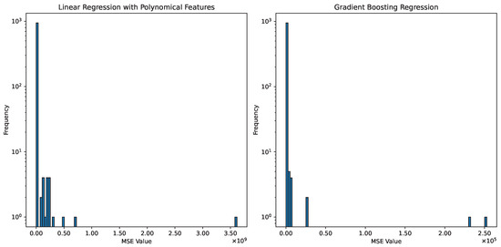
Figure 3.
Comparison of MSE for linear regression (with polynomial features) and gradient boosting regression on the raw data for all predictors in the dataset O.
For completeness, we also show the MSE distribution of regression for generating the missing data for the reference dataset in Figure 4. The primary purpose is still to demonstrate which regression model should be used to generate the missing data. Similar to the case for generating missing data in the dataset for our current study, GBR again outperforms LRPF with much smaller MSE for the reference dataset.
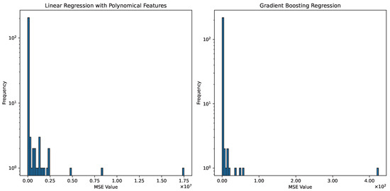
Figure 4.
Comparison of MSE for linear regression (with polynomial features) and gradient boosting regression on the raw data for all predictors in the reference dataset R.
5.2. Determination of the Weights of Predicators
The objective-weighting Python library (https://pypi.org/project/objective-weighting/) (accessed on 1 March 2025) is used as the basis for the calculation of the weights of the predictors. The reason why we cannot use that library as it is is because the entropy weighting function uses a sum normalization instead of the min-max normalization. The purpose of sum normalization is to scale the values in a vector so that the sum of the scaled values equals to 1. On the other hand, the min-max normalization would scale all values to a range between 0 and 1. Hence, for our study, the min-max normalization is used. The source code of the entropy weighting function in the objective-weighting python library is modified accordingly. The weights calculated this way are shown in Figure 5 for our dataset, and shown in Figure 6 for the reference dataset.
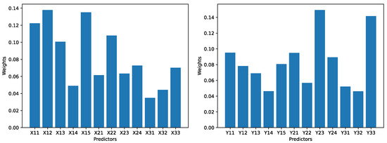
Figure 5.
The weights for 12 predictors for the technological innovation subsystem (left), and the weights for the 12 predictors for the financial development subsystem (right) in the dataset O.
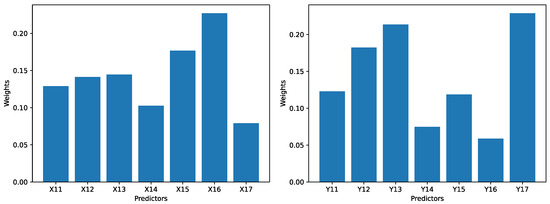
Figure 6.
The weights for 7 predictors for the technological innovation subsystem (left), and the weights for the 7 predictors for the financial development subsystem (right) in the dataset R.
As can be seen, for the technological innovation subsystem in dataset O, the largest weight is 0.138 (for ), and the smallest weight is 0.035 (for ). For the financial development subsystem in dataset O, the largest weight is 0.149 (for ), and the smallest weight is 0.046 (for ).
For the technological innovation subsystem in the dataset R, the largest weight is 0.227 (for ), and the smallest weight is 0.079 (for ). For the financial development subsystem in the dataset R, the largest weight is 0.229 (for ), and the smallest weight is 0.059 (for ).
The ratio between the largest weight and the smallest weight for all subsystems and for both datasets is roughly between 3 and 4. Hence, no predictor can be apparently ignored during the calculation for the comprehensive evaluation index. In other words, every predictor would make some impact to the comprehensive evaluation index to the subsystem, and eventually may exert some impact on the degree of coupling and degree of coordination.
5.3. Determination of Comprehensive Evaluation Index for Technological Innovation
In this section, we report the comprehensive evaluation index for the technological innovation subsystem. The complete calculated indices for all 30 regions in years 2002–2023 for dataset O is provided in Appendix B, Table A3. The complete indices for the reference dataset R are provided in Appendix B, Table A5.
First, we provide an overview of the indices for all 30 regions in 2002, 2012, and 2023, for the technological innovation subsystem calculated using dataset O in Figure 7.
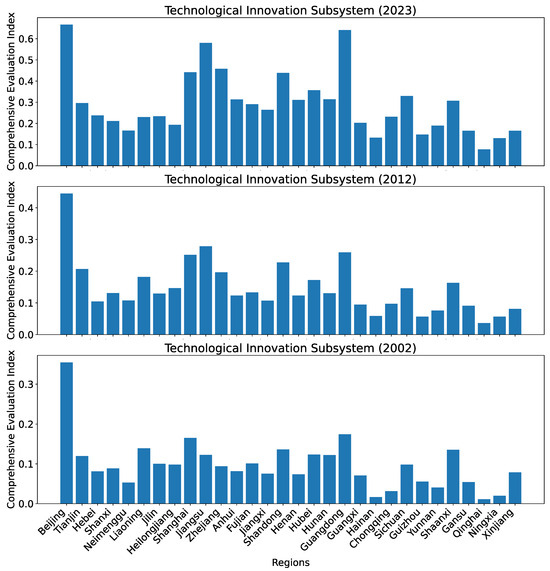
Figure 7.
Comprehensive evaluation indices for the technological innovation subsystem for all 30 regions in China in 2002, 2012, and 2023 calculated using dataset O.
To show the evolution of the indices over the years, we show two regions, Beijing, which consistently has the highest index, and Qinghai, which has the lowest index among all regions, in Figure 8. As can be seen, the general trend for both regions is that the development level (as indicated by the index) is increasing over time, with the exception of occasional slight drops (from 2002 to 2003 for Beijing) or stagnancy (from 2010 to 2011 for Beijing; from 2004 to 2005 and from 2014 to 2015 for Qinghai).
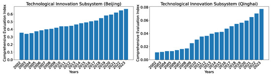
Figure 8.
Comprehensive evaluation indices for the technological innovation subsystem for Beijing and Qinghai over the years 2002–2023 calculated using dataset O.
For readers who are not familiar with China, it is necessary to provide some explanation regarding as to why Qinghai consistently has the lowest index and Beijing consistently has the highest index. Unlike many developed countries, regions in China may have huge differences in their development levels due to historical governmental policies, locations, natural and human resources. We contrast the two regions from four dimensions that could impact their development levels:
- Economic and financial infrastructure: Beijing is the capital of China with a large concentration of financial institutions, including international financial headquarters. Qinghai, on the other hand, is located in the far western region of China and much less economically developed with very limited financial infrastructure.
- Technological development: Beijing is home to many top universities in China, and as such, Beijing is leading in patent filings and technology startups. In contrast, Qinghai does not have a top university and lacks the high-tech industrial base.
- Government policy and investment: Being the capital of China, Beijing receives substantial central government funding and policy support. The support for Qinghai is limited to renewable energy projects.
- Human capital and talent pool: Due to the special location and the rich opportunities, Beijing attracts top-tier latent from across China. Beijing also has the best talent pool in China due to its top universities. In contrast, Qinghai faces significant challenges in attracting and retaining skilled workers due to the lack of opportunities and possibly harsh weather. Qinghai also lacks a talent pool.
As can be seen in Figure 9, the development levels across different regions appear rather similar when we use the set of seven predictors proposed in [3]. What is also odd is that Henan has the highest index value in 2002, and Hubei has the highest index value in 2023. The calculated distribution of the indices clearly fail to match the reality in China. Beijing, the capital city of China, has a concentration of the best higher educational institutions in China. As such, Beijing should be expected to have the highest technological innovation index. Henan and Hubei are nowhere near the level of Beijing. This demonstrates that the choice of the set of predictors is very important to deriving the development levels of each subsystem. The issue of using the set of seven predictors is further evident from the evolution of the indices over time as shown in Figure 10. Unlike the gradual but consistent increase in the development levels for Beijing and Qinghai from 2002 to 2023 shown in Figure 8, what is shown in Figure 10 implies that the development levels for Beijing and Qinghai in recent years (2007–2023) are basically stagnant, which clearly fail to reflect the reality because we all know the rapid technological development in China during that period.
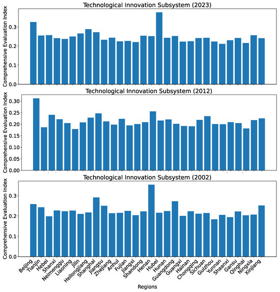
Figure 9.
Comprehensive evaluation indices for all 30 regions in China in 2002, 2012, and 2023 calculated using the reference dataset R.
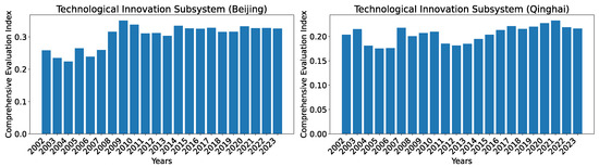
Figure 10.
Comprehensive evaluation indices for the technological innovation subsystem for Beijing and Qinghai over the years 2002–2023 calculated using the reference dataset R.
5.4. Determination of Comprehensive Evaluation Index for Financial Development
In this section, we report the comprehensive evaluation index for the financial development subsystem. The complete calculated index for all 30 regions in years 2002–2023 using our dataset O is provided in Appendix B, Table A4. The complete index using the reference dataset R for comparison is provided in Appendix B, Table A6. We provide an overview of the indices for all 30 regions in China in 2002, 2012, and 2023, for the financial development subsystem that is estimated using our set of 12 predictors in Figure 11. The calculated indices align with common knowledge of China’s financial development where Beijing, Shanghai, and Guangdong are the top three regions. In recent years, Jiangsu and Zhejiang are getting close to the levels of the top three regions.

Figure 11.
Comprehensive evaluation indices for the financial development subsystem for all 30 regions in China in 2002, 2012, and 2023 calculated using the dataset O.
To show the evolution of the indices over the years, we show two regions, Beijing, which consistently has the highest index, and Qinghai, which has the lowest index among all regions in year 2023, in Figure 12. As can be seen, the general trend for Beijing is that the development level (as indicated by the index) is increasing over the time but with more noticeable jittering compared with that of technological innovation. For Qinghai, even though the general trend is also roughly increasing over the years, we see episodes of declines (from 2005 to 2006; and from 2008 to 2010) and stagnancy (from 2018 to 2023).
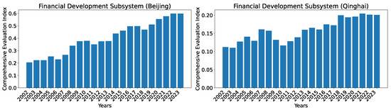
Figure 12.
Comprehensive evaluation indices for the financial development subsystem for Beijing and Qinghai over the years 2002–2023 calculated using the dataset O.
In comparison, the estimated development levels as shown in Figure 13 calculated using the reference dataset R are quite different from ours. Only Beijing still ranks the first in index value. Shanghai does not even rank among the top three. In year 2023, Shanghai is even ranked below Anhui, which does not match the reality. As can be seen in Figure 13, the development levels across different regions appear to be rather similar when we use the reference dataset R.
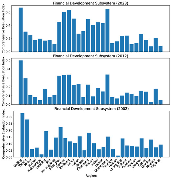
Figure 13.
Comprehensive evaluation indices for the financial development subsystem for all 30 regions in China in 2002, 2012, and 2023 calculated using the reference dataset R.
Again, the issues of using the set of seven predictors are evident from the evolution of the indices over time, as shown in Figure 14. For Beijing, the drastic increase in the development level from 2006 to 2007 is unrealistic. For Qinghai, there are also several apparent issues: (1) It is odd that the development level is already relatively high in 2002 (i.e., the second-highest index second only to the year 2020 value); (2) the drastic drop in development level from 2002 to 2003 cannot be explained; and (3) similarly, the huge drop in development level from year 2020 to year 2021 is also hard to explain.
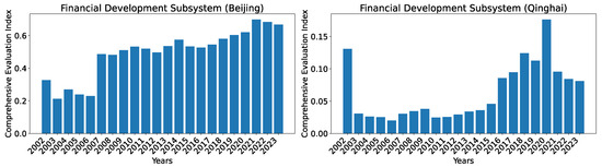
Figure 14.
Comprehensive evaluation indices for the financial development subsystem for Beijing and Qinghai over the years 2002–2023 calculated using the reference dataset R.
5.5. The Coupling Degree Between Technological Innovation and Financial Development
Figure 15 shows the coupling degrees between the technological innovation and the financial development subsystems calculated based on our set of 12 predictors for each subsystem for all 30 regions in 2002, 2012, and 2023.
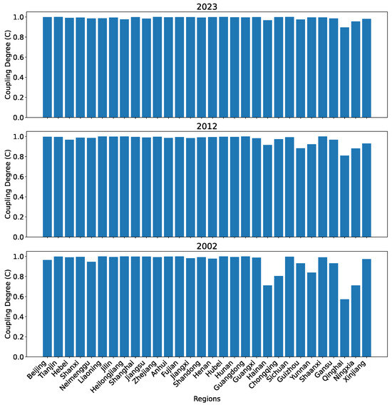
Figure 15.
The coupling degree between the two subsystems for all 30 regions in China in 2002, 2012, and 2023 calculated using dataset O.
As can be seen, except Qinghai, and to some extent Ningxia, the coupling degrees are very close to 1.0 in 2023. Back in 2002, the western areas in China have apparent imbalance in the development levels of the two subsystems. This imbalance has been improved over time. Overall, the coupling degrees appear to be consistent with the actual development in different regions in China. The evolution of the coupling degrees for Beijing and Qinghai over the years 2002–2023 is shown in Figure 16. Even in 2002, Beijing already had a high coupling degree between the two subsystems, and it stays high close to one through 2023. For Qinghai, the coupling degree rises from below 0.6 to over 0.9 over the years, with a noticeable increase over the span of three years (2008, 2009, and 2010).
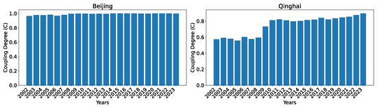
Figure 16.
The coupling degree between the two subsystems for Beijing and Qinghai over the years 2002–2023 calculated using dataset O.
The coupling degrees for the 30 regions in 2002, 2012, and 2023 using the seven predictors proposed in [3] for each subsystem are shown in Figure 17.
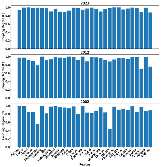
Figure 17.
The coupling degree between the two subsystems for all 30 regions in China in 2002, 2012, and 2023 calculated using the reference dataset R.
Although it is somewhat counterintuitive for Beijing to have a lower coupling degree than that for Tianjin, Hebei, and Shanxi, there is no strong evidence there is something wrong with the model itself. The evolution over the years for Beijing and Qinghai revealed serious issues as shown in Figure 18. First, one may notice that the coupling degree for Beijing is gradually reducing over the years, with that for 2023 apparently below that of year 2022. This does not match the reality where all regions in China have been improving their development levels in technological innovation as well as in financial development. Second, the coupling degree between the two subsystems for Qinghai appears to drop significantly from 2002 and 2003, which is not explainable. Both issues are evidence that the seven predictors ( to ) failed to fully capture the development levels of the technological innovation subsystem, and the seven predictors ( to ) failed to fully capture the development levels of the financial development subsystem.
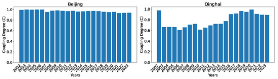
Figure 18.
The coupling degree between the two subsystems for Beijing and Qinghai over the years 2002–2023 calculated using the reference dataset R.
5.6. The Coordination Degree Between Technological Innovation and Financial Development
Figure 19 shows the coordination degrees between the technological innovation and the financial development subsystems calculated based on our dataset O for all 30 regions in 2002, 2012, and 2023. As can be seen, all regions have been improving their coordination degrees over the 21 years. The patterns of the coordination degrees for the regions are roughly aligned with expectation. In 2002, Beijing, Shanghai, and Guangdong have the highest coordination degrees and are higher than the remaining regions by a big margin. In 2012, Jiangsu and Zhejiang were catching up with Shanghai. In 2023, Jiangsu already surpassed Shanghai.
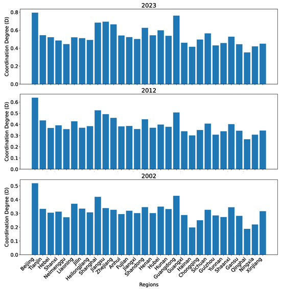
Figure 19.
The coordination degree between the two subsystems for all 30 regions in China in 2002, 2012, and 2023 calculated using our dataset O.
Figure 20 shows the evolution of the coupling degrees for Beijing and Qinghai over the years 2002–2023. Both Beijing and Qinghai had a steady increase in their coordination degree over the years. Beijing increased from slightly above 0.5 to close to 0.8. Qinghai increased from under 0.2 to close to 0.35.
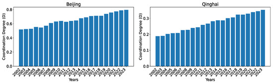
Figure 20.
The coordination degree between the two subsystems for Beijing and Qinghai over the years 2002–2023 calculated using our dataset O.
Figure 21 shows the coordination degrees for the 30 regions in 2002, 2012, and 2023 using the reference dataset R. Although the overall patterns of the coordination degrees contain no apparent issue, the increase in the coordination degrees over the years is less prominent than that predicted using our set of predictors.
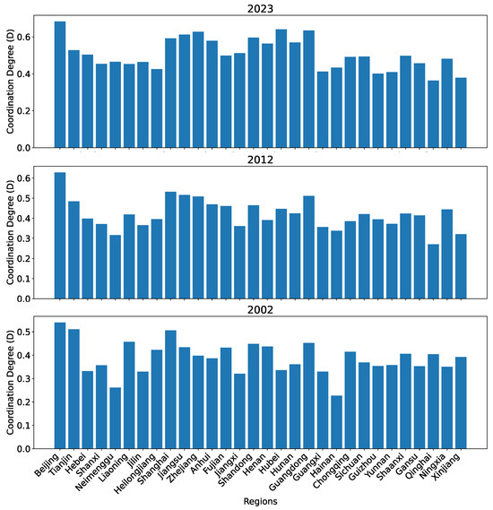
Figure 21.
The coordination degree between the two subsystems for all 30 regions in China in 2002, 2012, and 2023 calculated using the reference dataset R.
As shown in Figure 22, the evolution over the years for Beijing and Qinghai revealed more issues. First, for Beijing, other than a significant jump in coordination degree from 2006 to 2007, the coordination degrees are fairly stagnant, i.e., there were less than 0.1 increases from 2008 to 2023. This does not appear to match the rapid technological and financial development during this time period. Second, for Qinghai, the coordination degrees drop in three periods: (1) from 2002 to 2006, (2) from 2009 to 2011), and (3) from 2020 to 2023. There does not appear to be any reason for the drop in the first two periods. Perhaps the third period may be attributed to the pandemic. Again, the issues could be due to the set of predictors failing to capture the actual development level of each subsystem.
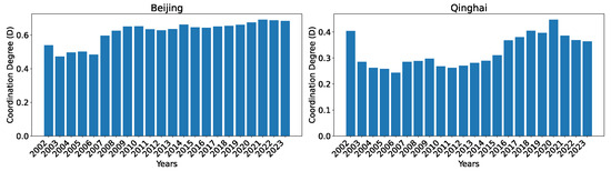
Figure 22.
The coordination degree between the two subsystems for Beijing and Qinghai over the years 2002–2023 calculated using the reference dataset R.
5.7. Projection of Future Coordination Degree
Highly reliable projection of future coordination degree could be very useful for enacting conducive policies to encourage coherent development in technological innovation and financial systems. In this subsection, we report our effort in making such projections. The findings prove that making the correct projection of future coordination degree is very challenging.
In our investigation, we would like to project for the most recent five years in our dataset, i.e., 2019, 2020, 2021, 2022, and 2023, using the remaining data as the training set for a regression model. The projection accuracy is evaluated using a metric called . This metric quantifies the normalized error between the predicted values and the actual values with one caveat, i.e., would be a negative number if the prediction is so bad that it is worse than simply making the prediction using a straight horizontal line. A perfect regression would have a (i.e., the regression model explains all the variability in the actual data around the mean), and a regression would have a if the model fails to explain any of the variability in the actual data.
We experiment with two regression models. One is linear regression with polynomial features. The other is gradient boosting regression. Again, we compare the results of the two sets of coordination degrees computed using the dataset O and the reference dataset R. The regression study is performed with three-fold cross-validation with hyperparameter tuning using grid search. For linear regression, a single hyperparameter, i.e., polynomial degree, with possible values of 1, 2, and 3, is tuned with cross-validation. For GBR, five hyperparameters are tuned with cross-validation:
- Number of estimators: with possible values of 50, 100, and 200;
- Learning rate: with possible values of 0.01, 0.1, and 0.2;
- Max depth: with possible values of 3, 4, 5;
- Minimum samples split: with possible values of 2, 5, and 10;
- Minimum samples leaf: with possible values of 1, 2, and 4.
5.7.1. Linear Regression with Polynomial Features
Figure 23 shows the results of the training and testing performance using using our dataset O. As can be seen, the high training performance does not translate to high testing performance at all. All but one region has a training greater than 0.9. However, 12 regions have negative testing . Only seven regions score greater than 0.8. This result means that one would have to be cautious when interpreting the projected coordination degrees, particularly when enacting development policies.

Figure 23.
LRPF training and testing for the coordination degrees using our dataset O.
In contrast, the training performance and testing performance for the coordination degrees using the reference dataset R are far worse as shown in Figure 24. Eight regions have very low training . Only six regions have training higher than 0.9. Furthermore, only two regions have positive testing . Again, our findings demonstrate that using inappropriate predictors would render unreliable results.
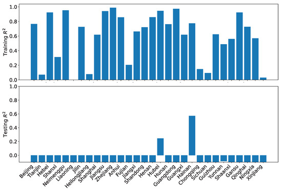
Figure 24.
LRPF training and testing for the coordination degrees using the reference dataset R.
For completeness, we show the actual coordination degree and the predicted value for two regions, Beijing and Sichuan, using our dataset O in Figure 25. Beijing has reasonably good project performance, while Sichuan has negative value. The insets are zoomed-in for the five-year projection.
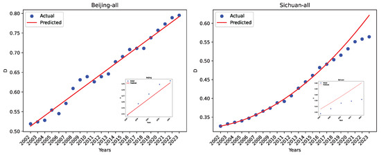
Figure 25.
The actual data and the LRPF-predicted values using our dataset O for Beijing and Sichuan.
Figure 26 shows the actual coordination degree and the predicted value for two regions, Hainan and Sichuan, using the reference dataset R. Hainan has the best project performance using dataset R, while Sichuan has a negative value. As can be seen, the regression errors are much larger than those using our dataset O.
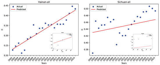
Figure 26.
The actual data and the LRPF-predicted values using the reference dataset R for Hainan and Sichuan.
Besides , the regression and projection performance can also be evaluated in terms of mean absolute error (MAE) and root mean squared error (RMSE). For completeness, we show the performance evaluation in terms of MAE and RMSE for both our dataset O and the reference dataset R in Figure 27, Figure 28, Figure 29 and Figure 30.
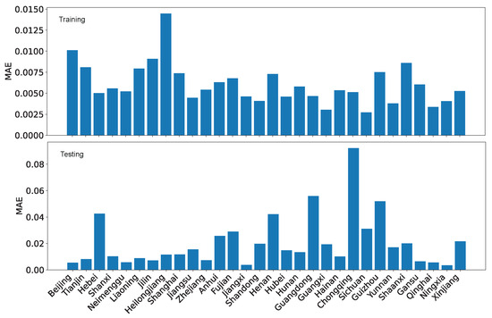
Figure 27.
LRPF training MAE and testing MAE for the coordination degrees using our dataset O.

Figure 28.
LRPF training MAE and testing MAE for the coordination degrees using the reference dataset R.
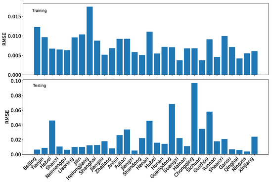
Figure 29.
LRPF training RMSE and testing RMSE for the coordination degrees using our dataset O.
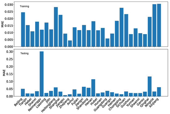
Figure 30.
LRPF training RMSE and testing RMSE for the coordination degrees using the reference dataset R.
Using MAE as the performance evaluation metric, we can see from Figure 27 and Figure 28 that the error is several folds bigger for the reference dataset R than for our dataset O. Furthermore, regardless of which dataset is used, the testing error is also bigger than the training error by several folds. Nevertheless, the difference is not enormous because the coordination degree is normalized within the range of [0,1].
Using RMSE as the performance evaluation metric, we can see from Figure 29 and Figure 30, the patterns are similar to those for MAE. However, the contrast is less for RMSE than for MAE due to how the error is calculated.
If we compare the evaluation results based on , we can conclude that is a more distinctive metric on the quality of regression and projection because the contrast between training and testing, as well as the contrast between the performance of the two datasets, is much more prominent.
5.7.2. Gradient Boosting Regression
Figure 31 shows the results of the training and testing performance using using our dataset O. As can be seen, the training performance is superb, with all but one region has nearly perfect . However, the generalizability is extremely poor, with the testing being negative for all regions. Obviously, the gradient boosting regression is not suitable for making projections.
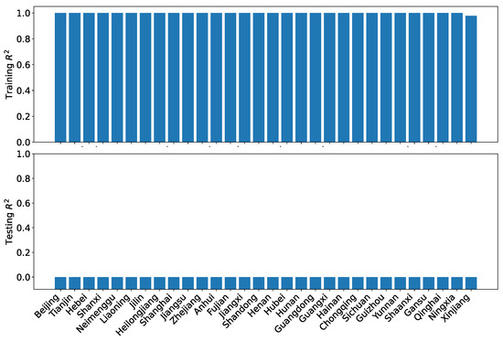
Figure 31.
GBR training and testing for the coordination degrees using our dataset O.
The patterns of performance on training and testing remain similar for the coordination degrees using the reference dataset R as shown in Figure 32. While the training performance is noticeably improved over the linear regression with polynomial features, the testing performance is actually worse, with no region having positive .
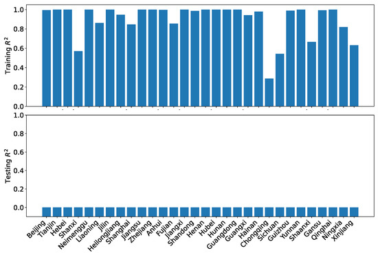
Figure 32.
GBR training and testing for the coordination degrees using the reference dataset R.
For completeness, we show the actual coordination degree and the predicted value for the same two regions, Beijing and Sichuan, using our dataset 0, in Figure 33. The insets are zoomed-in for the five-year projection. As can be seen, GBR has excellent regression performance for the training set but performs poorly for projection using the testing set.
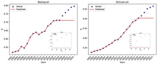
Figure 33.
The actual data and the GBR-predicted values using our dataset O for Beijing and Sichuan.
Figure 34 shows the actual coordination degree and the GBR-predicted value for two regions, Hainan and Sichuan, using the reference dataset R. As can be seen, again, the regression errors are much larger than those using our dataset O.
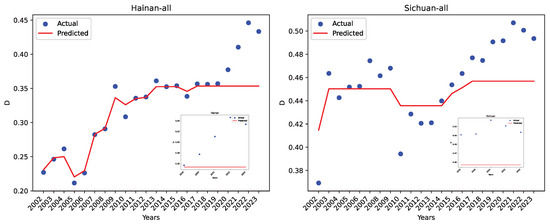
Figure 34.
The actual data and the GBR-predicted values using the reference dataset R for Hainan and Sichuan.
Similar to LRPF, besides , the regression and projection performance can also be evaluated in terms of mean absolute error (MAE) and root mean squared error (RMSE). For completeness, we show the performance evaluation in terms of MAE and RMSE, for both our dataset O and the reference dataset R in Figure 35, Figure 36, Figure 37 and Figure 38.
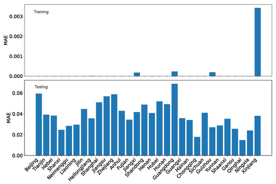
Figure 35.
GBR training MAE and testing MAE for the coordination degrees using our dataset O.
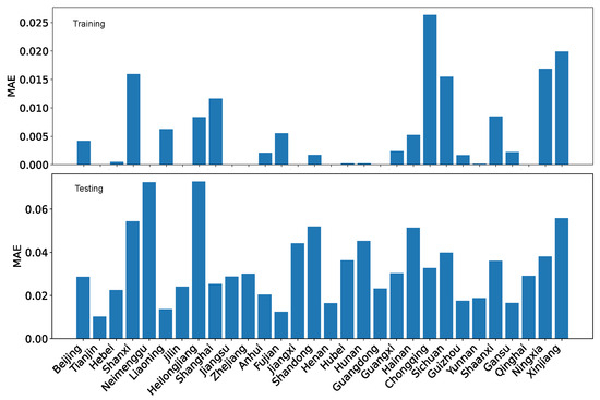
Figure 36.
GBR training MAE and testing MAE for the coordination degrees using the reference dataset R.
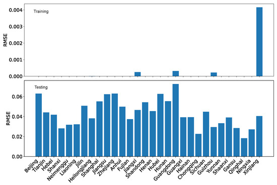
Figure 37.
GBR training RMSE and testing RMSE for the coordination degrees using our dataset O.
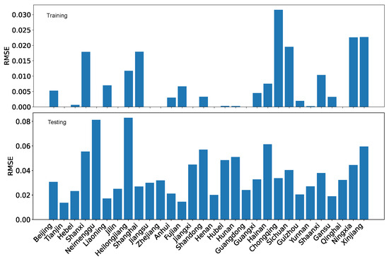
Figure 38.
GBR training RMSE and testing RMSE for the coordination degrees using the reference dataset R.
Using MAE as the performance evaluation metric, we can see from Figure 35 and Figure 36 that the training error is several folds bigger for the reference dataset R than for our dataset O. However, the testing errors for the two datasets are on the same scale.
Using RMSE as the performance evaluation metric, we can see from Figure 37 and Figure 38, the patterns are roughly similar to those for MAE. The testing error for the reference dataset R is slightly larger than that for our dataset O.
Again, we can see that is a more distinctive metric on the quality of regression and projection because the contrast between training and testing, as well as the contrast between the performance of the two datasets are much more prominent.
6. Discussion
In this section, we engage in in-depth discussion on several aspects of our study, including three alternative configurations (using a reduced predictor set, using alternative imputation methods, and using an alternative weighting method), and statistical comparison of the outcomes derived from different configurations, including using our dataset and the reference dataset.
6.1. Reduced Predictor Set
We are using 12 predictors for each subsystem, which is more than most other studies. It is desirable to determine which predictors are the most influential to the study of coupling and coordination degrees. This is typically performed via a sensitivity analysis. Because the weight for each predictor is calculated as the first step in our study, we choose to use weights as the indication for the most influential predictors. Because the reference dataset that we use employs seven predictors to model each subsystem, we decide to use the seven predictors that have the largest weights to calculate the comprehensive evaluation index for each subsystem, the degree of coupling, the degree of the coordination, and subsequently to make projection. The results are in general rather similar to those produced using the 12-predictor set for each subsystem. In Figure 39, we show the training performance and the testing performance for the coordination degrees using our dataset O using the reduced seven-predictor set for each subsystem. Compared with the result obtained using the full 12-predictor set, 12 regions have positive with the 7-predictor set while there are 18 regions have positive . Nevertheless, the result is significantly better than that using the reference dataset R, where only two regions have positive .
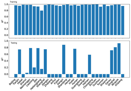
Figure 39.
LRPF training and testing for the coordination degrees using our dataset O using the reduced 7-predictor set for each subsystem.
6.2. Alternative Imputation Methods
In our study, we compare two imputation methods [49] for filling missing data, one is LRPF, and the other is GBR. We use the regression performance as an indicator to select which one is better. Because GBR has significantly smaller errors, we choose to use GBR to fill the missing data. Because other imputation methods are available [49], it will be interesting to experiment with these imputation methods. It is difficulty to compare the performance of imputation methods because we do not have complete dataset. We experiment with using the Kolmogorov–Smirnov (KS) test [50] to gauge the performance of imputation methods. If the imputation is doing a good job, the expectation is that the imputed data would have similar distribution to the original data, which would lead to a KS score of closing to 0. We test the following imputation methods: mean imputed, median imputed, mode imputed, forward fill, backward fill, KNN inputted, and interpolated. All imputation methods have rather similar low KS scores. Hence, comparing distributions is not informative. Instead, we single out the interpolated imputation method and compute the regression performance based on missing data filled by this method. The regression performance for LRPF and GBR is shown in Figure 40. As can be seen, the performance is degraded noticeably for both training and testing.
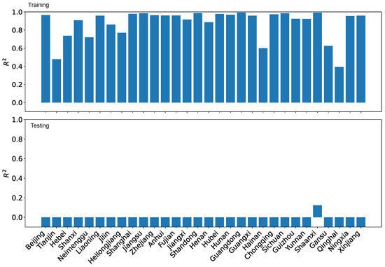
Figure 40.
LRPF training and testing for the coordination degrees using our dataset O, where the missing data are filled with the interpolated imputation method.
6.3. Alternative Weighting Method
Besides the entropy weighting, several other objective weighting methods are available. To examine the impact of weighting method to the results, we additionally experiment with the CRITIC method [33]. We visually compare the resulting comprehensive evaluation index for both subsystems, the degree of coupling, the degree of coordination, as well as the projection performance. They are rather similar to those computed using the entropy weighting method. In Figure 41, we show the training and testing regression performance for making projection.
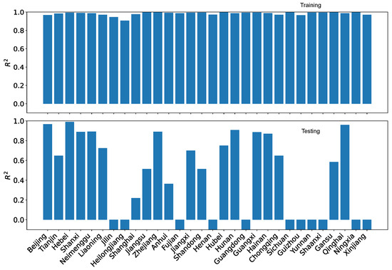
Figure 41.
LRPF training and testing for the coordination degrees using our dataset O, where the weights are calculated using the CRITIC weighting method.
6.4. Statistical Comparison of Regression Performance
In previous sections, we visually compared the regression results on the degree of coordination for the two datasets. In this subsection, we present a statistical comparison of the two datasets and demonstrate that indeed our dataset O has statistical better regression performance . Due to the presence of negative values in the testing results, we can only perform the statistical comparison using the training performance. We first check the values for each dataset for normality. If the distributions of for both datasets are both normal, then we can use the t-test. Otherwise, we compare using a form of non-parametric statistical method, i.e., confidence interval. The normality checks on the regression performance for both datasets for both LRPF and GBR fail. Hence, we have to resort to using confidence interval for statistical comparison.
We also take this opportunity to compare with several other configurations: (1) using the seven-predictor set for each subsystem based on our dataset O; (2) using the interpolated imputation method to fill the missing data; and (3) using CRITIC weighting method to calculate the weights. The comparison is made for both LRPF and GBR. As shown in Figure 42, all four different configurations using our dataset O are statically better than R because there is no overlap between the two confidence intervals. Three configurations (the original configuration with 12-predictor set for each subsystem, and alternative configurations 1 and 3) are statistically the same. However, the results are sensitive to the alternative interpolated imputation method, which lowers the performance when LRPF is used for regression. When GBR is used for regression, all four configurations are equivalent.
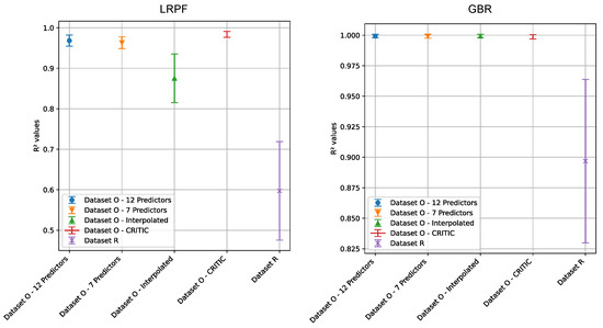
Figure 42.
Statistical comparison of the training performance for our dataset O in four different configurations and the reference dataset R, for both LPRF (left) and GBR (right).
6.5. Heterogeneity of Coordination Degrees and Heterogeneity of Projection Performance
As we have shown in previous sections, there is an apparent heterogeneity of the coordination degrees among different regions, and there is also an apparent heterogeneity of the projection performance. It is interesting to see if there is any correlation between the heterogeneity. We note that the regression performance in terms of is rather uniform across almost all regions. Hence, we choose to focus on the heterogeneity of the testing performance (i.e., project performance). The top 10 regions for the degree of coordination and the top 10 regions for the testing performance are shown in Figure 43 side-by-side. As labeled using colored arrows, four regions (Beijing, Zhejiang, Hubei, and Tianjin) are present in both plots. This demonstrates that the heterogeneity of the degree of coordination is not strongly correlated with the heterogeneity of the projection performance.
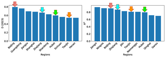
Figure 43.
The top 10 regions for the degree of coordination and the top 10 regions for the projection performance. The four regions that are present in both are highlighted.
7. Concluding Remarks
In this paper, we make a critical look at the mainstream approach in estimating the coupling and coordination of two or more subsystems from the engineering perspective. The mainstream approach is to define a set of predictors for each subsystem. Then, the weight for each predictor is calculated towards establishing the development level of the subsystem (referred to as comprehensive evaluation index in our study). Subsequently, the coupling degree and the coordination degree are computed based on the comprehensive evaluation indices of the subsystems. A big issue with this approach is the lack of validation of the results. The set of predictors is usually subjectively defined base on the authors’ expertise and perspective. As such, there is no guarantee that the set of predictors can fully model the subsystem. Consequently, the development level of each subsystem, and the following coupling degree and the coordination degree could be biased and misleading. While people who are familiar with the subsystems may have subjective perceptions regarding which regions are more developed, there is no established ground truth for validation.
While in this paper we focus on the coupling and coordination of technological innovation and financial development, the issue identified above is applicable to all similar studies. Hence, the impact of the issue is wider than the specific scope of our current study. The goal of this study is to explore the feasibility of establishing an objective evaluation method on the quality of the models for the subsystems via the regression and projection performance of the coordination degree between the subsystems. The hypothesis is that if the set of predictors defined is an accurate model for each subsystem, then the intrinsic interaction between the subsystems may be reliably estimated via regression. This would lead to small regression error on the training data, and good projection performance for the near future. By performing a side-by-side comparison between our dataset O (each subsystem is modeled with 12 predictors) and a reference dataset R (each subsystem is modeled with 7 predictors), we demonstrate the feasibility of objectively evaluate alternative models. Indeed, the set of predictors that we propose lead to significantly better regression and project performance than the approach that we use as a reference.
Limitations. Our study is the first step in establishing an objective evaluation method for the coupling and coordination studies of two or more subsystems. Due to the limited time and resources, we only compare our model with one reference system. Ideally, we should compare with all related studies, which would make the result much more compelling. Furthermore, we present a qualitative comparison. It is desirable to develop a systematic quantitative evaluation method where one or more metrics are defined. Additionally, the scope could be extended beyond regions in China to other developing countries, provided that the data are available.
We also acknowledge that the selection of 12 predictors for each subsystem is quite subjective. How to determine what predictors to use to fully describe the subsystem is still an open research issue. Furthermore, assessment on the potential redundancy and multicollinearity of the predictors is also desirable. Unfortunately, in the context of financial development, it is unclear how to perform the assessment due to the lack of ground truth regarding the degree of coupling and the degree of coordination.
The current study is limited in its analysis of the relationship between the development levels of two subsystems. In future work, we plan to explore potential causal relationships development levels of the two subsystems and their coordination degree could deepen the study’s implications. For instance, Granger causality tests [51] could help determine whether changes in one subsystem can forecast changes in the other or in the coordination degree. Furthermore, given the panel structure of the data (regions over time), applying panel regression techniques [52] (e.g., fixed or random effects models) could help account for unobserved regional heterogeneity and yield more robust estimates of the interrelationships. This would also clarify whether the determinants of coordination are consistent across regions.
Last, but not least, the use of regression performance as a benchmark for evaluating the models for the coordination of subsystems for financial development, although intuitive, lacks theoretical foundations. In particular, high regression performance alone might not be a fair evaluation of the coordination degrees of a model. Additional information should be collected, such as that related to policy relevance and external consistency, to fully evaluate a model.
Author Contributions
Conceptualization, J.Z., Y.J., Y.Y. and W.Z.; methodology, J.Z. and W.Z.; literature selection, J.Z., Y.J., Y.Y. and W.Z.; investigation, J.Z., Y.J., Y.Y. and W.Z.; writing—original draft preparation, J.Z., Y.J., Y.Y. and W.Z.; writing—review and editing, J.Z., Y.J., Y.Y. and W.Z.; visualization, W.Z. All authors have read and agreed to the published version of the manuscript.
Funding
This research received no external funding.
Institutional Review Board Statement
Not applicable.
Informed Consent Statement
Not applicable.
Data Availability Statement
The datasets and all the Python scripts are made available as a GitHub project (https://github.com/wenbingcsu/ccd, accessed on 1 May 2025).
Acknowledgments
We sincerely thank the reviewers for their insightful constructive criticism and invaluable suggestions, which greatly improved this paper.
Conflicts of Interest
The authors declare no conflicts of interest.
Abbreviations
The following abbreviations are used in this manuscript:
| LRPF | Linear Regression with Polynomial Features |
| GBR | Gradient Boosting Regression |
| MSE | Mean Squared Error |
| MAE | Mean Absolute Error |
| RMSE | Root Mean Squared Error |
| GDP | Gross Domestic Product |
| R&D | Research and Development |
| IQR | Interquartile Range |
| CRITIC | Criteria Importance Through Intercriteria Correlation |
Appendix A. Predictors Used for Subsystems in Related Studies
In this appendix, we provide the predictors used for subsystems in competing studies. To facilitate the comparison between the predictors used in different studies, we group the predictors for the technological innovation subsystem and the financial development subsystem separately in Table A1 and Table A2. As can be seen, the most common categories for the technological innovation subsystem are investment on technology, technological innovation environment, and technological innovation output. The most common categories for the financial development subsystem are financial development scale, financial development structure, and financial development efficiency.
Table A1.
Categories and predictors used for the technological innovation subsystem.
Table A1.
Categories and predictors used for the technological innovation subsystem.
| References | Category | Predictor |
|---|---|---|
| [3] | Investment on technology | Number of full-time R&D personnel () |
| R&D expenditure as percentage of GDP () | ||
| Financial investment in technology as percentage of GDP () | ||
| Technological innovation output | Number of patents applications () | |
| Number of technological papers indexed () | ||
| High tech transaction total amount () | ||
| New product sales as a percentage of total sales () | ||
| [4] | Investment on technology | Number of full-time R&D personnel |
| R & D investment as percentage of GDP | ||
| technological innovation environment | Number of patent applications | |
| Number of trademark applications | ||
| Intellectual property expenditure | ||
| Technological innovation output | Number of journal articles published | |
| High tech product export as a percentage of total export | ||
| [5] | Investment on technology | Number of full-time R&D personnel |
| R&D expenditure as percentage of GDP | ||
| Technological innovation output | Number of patent applications | |
| Number of patents awarded | ||
| [26] | The number of patents awarded | |
| Number of papers published | ||
| Wealth generated by high-tech industry as a percentage of the total industry valuation | ||
| Technology market contract valuation | ||
| [6] | Investment on technology | Number of full-time R&D personnel |
| R&D expenditure | ||
| Technological innovation environment | R&D funding as a percentage of the total fiscal expenditure | |
| Total high tech sales income as percentage of GDP | ||
| Total high-tech market value per 10,000 population | ||
| Technological innovation output | Number of publications indexed by SCI per 10,000 full-time R&D personnel | |
| Number of patents awarded per 100,000,000 RMB R&D expenditure | ||
| Total sales amount for new products as a percentage of all sales | ||
| [8] | Investment on technology | Number of full-time R&D personnel |
| The number of technological research institutions | ||
| Technological innovation environment | R&D funding as a percentage of the total fiscal expenditure | |
| Technological innovation output | Number of patents awarded | |
| The high-tech industry output value | ||
| [9] | Investment on technology | Number of R&D projects |
| R&D expenditure in industry | ||
| Technological innovation output | Number of patents applications | |
| Number of publications | ||
| New product output value | ||
| Technology transfer transaction amount | ||
| [27] | Investment on technology | Number of full-time R&D personnel |
| R&D expenditure | ||
| Technological innovation output | Total transaction amount in high-tech market | |
| Number of patents awarded | ||
| Total sales amount for new products | ||
| Technological innovation environment | Number of students enrolled in higher education per 100,000 population | |
| Number of households that have wide-band Internet connection | ||
| Number of technological research institutions | ||
| [25] | Investment on technology | Number of full-time R&D personnel |
| R&D expenditure | ||
| Actual amount of foreign capital used | ||
| Electricity consumption of the whole society | ||
| Total number of students in higher education | ||
| Technological innovation output | Innovation index | |
| Number of patents awarded | ||
| Technological innovation environment | Number of books in library per 1 million population | |
| Number of households that have wide-band Internet connection | ||
| Number of higher education institutions |
Table A2.
Categories and predictors used for the financial development subsystem.
Table A2.
Categories and predictors used for the financial development subsystem.
| References | Category | Predictor |
|---|---|---|
| [3] | Financial development scale | Financial industry output value () |
| Total financial assets as percentage of GDP () | ||
| Financial employment as percentage of total employment () | ||
| Financial development structure | Banking market share () | |
| Securities Industry Market Share () | ||
| Insurance market share () | ||
| Financial services efficiency | Loan-to-deposit ratio of financial institutions ( | |
| [4] | Financial environment | Protection extent for financial activities |
| Information acquisition for financial activities | ||
| Credit provided by banks as a percentage of GDP | ||
| Financial market | Stock exchange rate | |
| Stock exchange total as percentage of GDP | ||
| Public company marks cap as percentage of GDP | ||
| [5] | Financial support for technological innovation | Budget on R&D as percentage of total budget of local government |
| Financial development scale | Deposit balance of foreign currency | |
| Financial development structure | Total premium income | |
| [26] | Total value of financial assets as percentage of GDP | |
| Total near money as percentage of GDP | ||
| The ratio of total value of financial assets versus M1 | ||
| [8] | Financial development scale | Financial industry output as a percentage of GDP |
| Number of full-time personnel as a percentage of full-time personnel of all industries | ||
| Financial development structure | The proportion of equity financing to various loans | |
| Financial development efficiency | Ratio of various loans to deposits | |
| Financial industry output per capita | ||
| [6] | Financial development scale | Number of financial institutions per 10,000 population |
| The sum of load balance, stock market value, and premium income as a percentage of GDP | ||
| The sum of new loans, stock market financing amount, and bond financing amount as a percentage of GDP | ||
| Financial development structure | New loans as a percentage of GDP | |
| Term-life insurance premium income | ||
| financial development efficiency | The proportion of financial industry value added to total financial industry assets | |
| The proportion of loan balance to deposit balance of financial institutions | ||
| Stock turnover as a percentage of GDP | ||
| [27] | Fundamental condition | Fixed asset in financial industry |
| Increase in employment in the financial industry | ||
| Number of full-time personnel in the financial industry | ||
| Total wages of the personnel in the financial industry | ||
| Market status | Savings balance in banking institutions | |
| Loan balance in banking institutions | ||
| Total market value of stocks | ||
| Number of publicly-traded companies | ||
| Total Insurance premium income | ||
| [25] | Financial development scale | Total industrial output value |
| Gross regional product | ||
| Fixed asset investment | ||
| Year-end population | ||
| Fixed asset investment | ||
| Total retail sales of consumer goods | ||
| Financial benefit level | Number of public companies | |
| Loan balance of financial institutions at the end of the year | ||
| Deposit balance of financial institutions at the end of the year | ||
| The proportion of tertiary industry in GDP | ||
| Green finance considerations | Industrial wastewater discharge | |
| Industrial discharge | ||
| Industrial smoke and dust emissions |
Appendix B. Comprehensive Evaluation Index Results
In this appendix, we provide the full results of the comprehensive evaluation index for the technological innovation subsystem, that for the financial development subsystem, using both our dataset O and the reference dataset R, in Table A3, Table A4, Table A5 and Table A6, respectively.
Table A3.
The comprehensive evaluation index for the technological innovation subsystem using our dataset O.
Table A3.
The comprehensive evaluation index for the technological innovation subsystem using our dataset O.
| Region/Year | 2002 | 2003 | 2004 | 2005 | 2006 | 2007 | 2008 | 2009 | 2010 | 2011 | 2012 | 2013 | 2014 | 2015 | 2016 | 2017 | 2018 | 2019 | 2020 | 2021 | 2022 | 2023 |
|---|---|---|---|---|---|---|---|---|---|---|---|---|---|---|---|---|---|---|---|---|---|---|
| Beijing | 0.355 | 0.339 | 0.349 | 0.373 | 0.386 | 0.4 | 0.406 | 0.42 | 0.439 | 0.439 | 0.445 | 0.463 | 0.479 | 0.49 | 0.504 | 0.515 | 0.546 | 0.581 | 0.593 | 0.619 | 0.648 | 0.666 |
| Tianjin | 0.12 | 0.123 | 0.129 | 0.147 | 0.16 | 0.165 | 0.176 | 0.181 | 0.185 | 0.196 | 0.207 | 0.218 | 0.224 | 0.23 | 0.234 | 0.227 | 0.233 | 0.224 | 0.241 | 0.261 | 0.28 | 0.296 |
| Hebei | 0.081 | 0.082 | 0.084 | 0.088 | 0.071 | 0.065 | 0.072 | 0.079 | 0.087 | 0.096 | 0.105 | 0.116 | 0.124 | 0.129 | 0.142 | 0.156 | 0.164 | 0.173 | 0.186 | 0.2 | 0.22 | 0.237 |
| Shanxi | 0.089 | 0.088 | 0.09 | 0.097 | 0.104 | 0.1 | 0.106 | 0.114 | 0.118 | 0.125 | 0.131 | 0.138 | 0.141 | 0.142 | 0.145 | 0.149 | 0.154 | 0.152 | 0.162 | 0.179 | 0.195 | 0.211 |
| Neimenggu | 0.053 | 0.054 | 0.055 | 0.063 | 0.066 | 0.063 | 0.071 | 0.081 | 0.089 | 0.1 | 0.108 | 0.115 | 0.121 | 0.123 | 0.124 | 0.118 | 0.12 | 0.121 | 0.127 | 0.139 | 0.155 | 0.166 |
| Liaoning | 0.139 | 0.141 | 0.146 | 0.155 | 0.16 | 0.138 | 0.147 | 0.156 | 0.166 | 0.174 | 0.182 | 0.194 | 0.201 | 0.199 | 0.198 | 0.208 | 0.169 | 0.174 | 0.188 | 0.203 | 0.215 | 0.23 |
| Jilin | 0.1 | 0.1 | 0.102 | 0.11 | 0.097 | 0.099 | 0.105 | 0.116 | 0.118 | 0.121 | 0.129 | 0.136 | 0.143 | 0.149 | 0.151 | 0.153 | 0.155 | 0.154 | 0.168 | 0.178 | 0.199 | 0.234 |
| Heilongjiang | 0.098 | 0.102 | 0.104 | 0.212 | 0.118 | 0.12 | 0.128 | 0.135 | 0.139 | 0.142 | 0.147 | 0.151 | 0.154 | 0.155 | 0.151 | 0.153 | 0.149 | 0.141 | 0.152 | 0.161 | 0.185 | 0.193 |
| Shanghai | 0.165 | 0.17 | 0.178 | 0.185 | 0.202 | 0.218 | 0.233 | 0.251 | 0.253 | 0.26 | 0.252 | 0.268 | 0.275 | 0.283 | 0.298 | 0.313 | 0.335 | 0.354 | 0.367 | 0.397 | 0.416 | 0.442 |
| Jiangsu | 0.122 | 0.127 | 0.134 | 0.147 | 0.156 | 0.155 | 0.189 | 0.21 | 0.231 | 0.254 | 0.279 | 0.302 | 0.315 | 0.335 | 0.359 | 0.383 | 0.415 | 0.447 | 0.477 | 0.524 | 0.55 | 0.58 |
| Zhejiang | 0.094 | 0.099 | 0.106 | 0.12 | 0.13 | 0.127 | 0.149 | 0.159 | 0.173 | 0.181 | 0.196 | 0.217 | 0.229 | 0.244 | 0.274 | 0.282 | 0.311 | 0.342 | 0.362 | 0.391 | 0.417 | 0.458 |
| Anhui | 0.081 | 0.083 | 0.084 | 0.089 | 0.081 | 0.074 | 0.081 | 0.091 | 0.1 | 0.109 | 0.123 | 0.138 | 0.145 | 0.151 | 0.173 | 0.18 | 0.192 | 0.209 | 0.227 | 0.254 | 0.286 | 0.313 |
| Fujian | 0.101 | 0.106 | 0.108 | 0.115 | 0.123 | 0.083 | 0.093 | 0.103 | 0.11 | 0.123 | 0.133 | 0.147 | 0.159 | 0.167 | 0.182 | 0.191 | 0.204 | 0.222 | 0.235 | 0.257 | 0.273 | 0.291 |
| Jiangxi | 0.075 | 0.078 | 0.079 | 0.089 | 0.102 | 0.084 | 0.087 | 0.09 | 0.096 | 0.1 | 0.107 | 0.115 | 0.123 | 0.132 | 0.147 | 0.158 | 0.166 | 0.181 | 0.199 | 0.22 | 0.243 | 0.264 |
| Shandong | 0.136 | 0.139 | 0.142 | 0.154 | 0.148 | 0.154 | 0.172 | 0.182 | 0.199 | 0.213 | 0.228 | 0.243 | 0.252 | 0.269 | 0.284 | 0.3 | 0.308 | 0.312 | 0.346 | 0.38 | 0.407 | 0.439 |
| Henan | 0.073 | 0.075 | 0.076 | 0.083 | 0.084 | 0.077 | 0.087 | 0.097 | 0.107 | 0.115 | 0.123 | 0.134 | 0.145 | 0.153 | 0.174 | 0.193 | 0.203 | 0.222 | 0.237 | 0.261 | 0.287 | 0.311 |
| Hubei | 0.124 | 0.127 | 0.126 | 0.135 | 0.143 | 0.126 | 0.137 | 0.146 | 0.154 | 0.162 | 0.172 | 0.185 | 0.194 | 0.201 | 0.21 | 0.22 | 0.231 | 0.251 | 0.262 | 0.29 | 0.321 | 0.357 |
| Hunan | 0.122 | 0.123 | 0.125 | 0.132 | 0.138 | 0.087 | 0.098 | 0.108 | 0.114 | 0.121 | 0.131 | 0.14 | 0.146 | 0.155 | 0.163 | 0.175 | 0.189 | 0.205 | 0.229 | 0.25 | 0.282 | 0.314 |
| Guangdong | 0.174 | 0.175 | 0.177 | 0.188 | 0.196 | 0.154 | 0.184 | 0.202 | 0.225 | 0.24 | 0.259 | 0.287 | 0.297 | 0.331 | 0.371 | 0.414 | 0.457 | 0.51 | 0.538 | 0.585 | 0.608 | 0.641 |
| Guangxi | 0.071 | 0.072 | 0.072 | 0.075 | 0.064 | 0.059 | 0.065 | 0.07 | 0.08 | 0.087 | 0.095 | 0.102 | 0.108 | 0.111 | 0.12 | 0.13 | 0.135 | 0.147 | 0.158 | 0.175 | 0.188 | 0.203 |
| Hainan | 0.016 | 0.016 | 0.018 | 0.022 | 0.025 | 0.026 | 0.034 | 0.041 | 0.049 | 0.055 | 0.059 | 0.064 | 0.068 | 0.07 | 0.074 | 0.077 | 0.08 | 0.087 | 0.093 | 0.107 | 0.118 | 0.133 |
| Chongqing | 0.032 | 0.034 | 0.037 | 0.045 | 0.054 | 0.053 | 0.06 | 0.07 | 0.079 | 0.088 | 0.097 | 0.108 | 0.117 | 0.128 | 0.146 | 0.153 | 0.162 | 0.173 | 0.184 | 0.2 | 0.216 | 0.231 |
| Sichuan | 0.098 | 0.102 | 0.1 | 0.108 | 0.112 | 0.103 | 0.109 | 0.117 | 0.129 | 0.135 | 0.146 | 0.158 | 0.172 | 0.184 | 0.199 | 0.212 | 0.231 | 0.253 | 0.274 | 0.299 | 0.313 | 0.33 |
| Guizhou | 0.055 | 0.056 | 0.056 | 0.059 | 0.063 | 0.035 | 0.035 | 0.039 | 0.043 | 0.047 | 0.057 | 0.063 | 0.07 | 0.078 | 0.088 | 0.099 | 0.11 | 0.12 | 0.128 | 0.135 | 0.14 | 0.148 |
| Yunnan | 0.041 | 0.041 | 0.041 | 0.047 | 0.049 | 0.051 | 0.055 | 0.055 | 0.064 | 0.069 | 0.076 | 0.082 | 0.089 | 0.095 | 0.106 | 0.118 | 0.123 | 0.136 | 0.147 | 0.159 | 0.172 | 0.189 |
| Shaanxi | 0.135 | 0.132 | 0.133 | 0.14 | 0.129 | 0.12 | 0.126 | 0.137 | 0.145 | 0.153 | 0.163 | 0.177 | 0.185 | 0.192 | 0.201 | 0.209 | 0.218 | 0.228 | 0.24 | 0.263 | 0.285 | 0.307 |
| Gansu | 0.054 | 0.054 | 0.054 | 0.061 | 0.065 | 0.064 | 0.069 | 0.074 | 0.079 | 0.084 | 0.091 | 0.098 | 0.102 | 0.105 | 0.108 | 0.109 | 0.113 | 0.115 | 0.123 | 0.135 | 0.15 | 0.165 |
| Qinghai | 0.011 | 0.012 | 0.013 | 0.013 | 0.015 | 0.016 | 0.017 | 0.025 | 0.031 | 0.035 | 0.036 | 0.04 | 0.042 | 0.042 | 0.047 | 0.051 | 0.055 | 0.056 | 0.059 | 0.065 | 0.07 | 0.077 |
| Ningxia | 0.02 | 0.02 | 0.021 | 0.025 | 0.033 | 0.036 | 0.034 | 0.04 | 0.045 | 0.053 | 0.057 | 0.064 | 0.069 | 0.072 | 0.075 | 0.08 | 0.086 | 0.092 | 0.098 | 0.107 | 0.113 | 0.13 |
| Xinjiang | 0.079 | 0.079 | 0.081 | 0.083 | 0.086 | 0.06 | 0.063 | 0.066 | 0.07 | 0.076 | 0.081 | 0.088 | 0.092 | 0.094 | 0.098 | 0.102 | 0.107 | 0.114 | 0.119 | 0.132 | 0.146 | 0.165 |
Table A4.
The comprehensive evaluation index for the financial development subsystem using our dataset O.
Table A4.
The comprehensive evaluation index for the financial development subsystem using our dataset O.
| Region/Year | 2002 | 2003 | 2004 | 2005 | 2006 | 2007 | 2008 | 2009 | 2010 | 2011 | 2012 | 2013 | 2014 | 2015 | 2016 | 2017 | 2018 | 2019 | 2020 | 2021 | 2022 | 2023 |
|---|---|---|---|---|---|---|---|---|---|---|---|---|---|---|---|---|---|---|---|---|---|---|
| Beijing | 0.205 | 0.223 | 0.223 | 0.253 | 0.229 | 0.266 | 0.339 | 0.376 | 0.379 | 0.35 | 0.375 | 0.377 | 0.438 | 0.461 | 0.497 | 0.498 | 0.469 | 0.51 | 0.555 | 0.577 | 0.598 | 0.598 |
| Tianjin | 0.103 | 0.127 | 0.122 | 0.114 | 0.12 | 0.165 | 0.162 | 0.185 | 0.154 | 0.161 | 0.173 | 0.185 | 0.178 | 0.203 | 0.223 | 0.212 | 0.229 | 0.253 | 0.278 | 0.288 | 0.296 | 0.296 |
| Hebei | 0.106 | 0.095 | 0.099 | 0.1 | 0.109 | 0.148 | 0.163 | 0.16 | 0.158 | 0.163 | 0.175 | 0.207 | 0.232 | 0.241 | 0.259 | 0.265 | 0.273 | 0.289 | 0.306 | 0.306 | 0.311 | 0.309 |
| Shanxi | 0.108 | 0.118 | 0.123 | 0.109 | 0.116 | 0.161 | 0.169 | 0.176 | 0.166 | 0.171 | 0.18 | 0.215 | 0.221 | 0.23 | 0.253 | 0.254 | 0.248 | 0.258 | 0.28 | 0.271 | 0.264 | 0.262 |
| Neimenggu | 0.103 | 0.101 | 0.099 | 0.097 | 0.099 | 0.135 | 0.132 | 0.142 | 0.135 | 0.139 | 0.152 | 0.162 | 0.165 | 0.168 | 0.173 | 0.211 | 0.212 | 0.223 | 0.244 | 0.241 | 0.239 | 0.237 |
| Liaoning | 0.134 | 0.136 | 0.142 | 0.137 | 0.157 | 0.189 | 0.174 | 0.19 | 0.17 | 0.184 | 0.185 | 0.248 | 0.223 | 0.248 | 0.271 | 0.297 | 0.315 | 0.323 | 0.352 | 0.365 | 0.32 | 0.319 |
| Jilin | 0.125 | 0.127 | 0.104 | 0.093 | 0.113 | 0.165 | 0.157 | 0.159 | 0.137 | 0.133 | 0.145 | 0.17 | 0.163 | 0.177 | 0.229 | 0.202 | 0.219 | 0.258 | 0.275 | 0.239 | 0.295 | 0.292 |
| Heilongjiang | 0.091 | 0.099 | 0.099 | 0.103 | 0.113 | 0.202 | 0.185 | 0.176 | 0.137 | 0.152 | 0.149 | 0.19 | 0.182 | 0.194 | 0.23 | 0.208 | 0.246 | 0.298 | 0.307 | 0.312 | 0.302 | 0.3 |
| Shanghai | 0.187 | 0.208 | 0.202 | 0.209 | 0.227 | 0.27 | 0.281 | 0.289 | 0.298 | 0.313 | 0.304 | 0.32 | 0.348 | 0.391 | 0.408 | 0.409 | 0.403 | 0.435 | 0.459 | 0.483 | 0.491 | 0.495 |
| Jiangsu | 0.107 | 0.134 | 0.15 | 0.144 | 0.165 | 0.172 | 0.19 | 0.189 | 0.179 | 0.193 | 0.209 | 0.235 | 0.251 | 0.274 | 0.305 | 0.321 | 0.327 | 0.34 | 0.363 | 0.385 | 0.401 | 0.4 |
| Zhejiang | 0.121 | 0.139 | 0.162 | 0.157 | 0.158 | 0.196 | 0.196 | 0.204 | 0.196 | 0.2 | 0.225 | 0.285 | 0.259 | 0.285 | 0.299 | 0.339 | 0.351 | 0.382 | 0.401 | 0.423 | 0.426 | 0.425 |
| Anhui | 0.092 | 0.106 | 0.107 | 0.113 | 0.123 | 0.139 | 0.159 | 0.157 | 0.158 | 0.159 | 0.173 | 0.21 | 0.147 | 0.218 | 0.238 | 0.243 | 0.242 | 0.233 | 0.25 | 0.263 | 0.272 | 0.271 |
| Fujian | 0.102 | 0.103 | 0.105 | 0.124 | 0.123 | 0.146 | 0.152 | 0.156 | 0.152 | 0.157 | 0.167 | 0.207 | 0.146 | 0.199 | 0.216 | 0.244 | 0.245 | 0.246 | 0.265 | 0.276 | 0.26 | 0.258 |
| Jiangxi | 0.111 | 0.108 | 0.101 | 0.091 | 0.102 | 0.146 | 0.151 | 0.145 | 0.135 | 0.139 | 0.153 | 0.175 | 0.174 | 0.187 | 0.19 | 0.193 | 0.213 | 0.214 | 0.232 | 0.235 | 0.24 | 0.24 |
| Shandong | 0.104 | 0.113 | 0.112 | 0.113 | 0.14 | 0.157 | 0.15 | 0.162 | 0.154 | 0.161 | 0.174 | 0.218 | 0.213 | 0.233 | 0.258 | 0.282 | 0.296 | 0.311 | 0.341 | 0.353 | 0.351 | 0.349 |
| Henan | 0.114 | 0.093 | 0.092 | 0.093 | 0.063 | 0.142 | 0.142 | 0.15 | 0.145 | 0.143 | 0.153 | 0.175 | 0.186 | 0.215 | 0.232 | 0.248 | 0.255 | 0.256 | 0.269 | 0.288 | 0.28 | 0.28 |
| Hubei | 0.12 | 0.119 | 0.125 | 0.122 | 0.121 | 0.154 | 0.143 | 0.135 | 0.136 | 0.134 | 0.147 | 0.168 | 0.187 | 0.198 | 0.221 | 0.225 | 0.238 | 0.244 | 0.261 | 0.268 | 0.275 | 0.358 |
| Hunan | 0.098 | 0.102 | 0.111 | 0.107 | 0.116 | 0.15 | 0.151 | 0.137 | 0.126 | 0.14 | 0.156 | 0.177 | 0.186 | 0.193 | 0.215 | 0.218 | 0.225 | 0.227 | 0.249 | 0.256 | 0.266 | 0.265 |
| Guangdong | 0.192 | 0.189 | 0.186 | 0.179 | 0.188 | 0.198 | 0.204 | 0.219 | 0.226 | 0.234 | 0.255 | 0.308 | 0.295 | 0.34 | 0.371 | 0.412 | 0.436 | 0.466 | 0.51 | 0.537 | 0.526 | 0.523 |
| Guangxi | 0.097 | 0.101 | 0.095 | 0.097 | 0.12 | 0.138 | 0.129 | 0.127 | 0.113 | 0.123 | 0.137 | 0.147 | 0.157 | 0.166 | 0.176 | 0.179 | 0.2 | 0.205 | 0.214 | 0.225 | 0.224 | 0.222 |
| Hainan | 0.094 | 0.1 | 0.105 | 0.105 | 0.098 | 0.12 | 0.123 | 0.135 | 0.119 | 0.135 | 0.139 | 0.146 | 0.191 | 0.184 | 0.201 | 0.191 | 0.198 | 0.198 | 0.206 | 0.218 | 0.228 | 0.223 |
| Chongqing | 0.124 | 0.121 | 0.117 | 0.117 | 0.118 | 0.147 | 0.151 | 0.155 | 0.156 | 0.15 | 0.154 | 0.185 | 0.199 | 0.226 | 0.236 | 0.229 | 0.349 | 0.233 | 0.246 | 0.251 | 0.262 | 0.26 |
| Sichuan | 0.115 | 0.12 | 0.127 | 0.124 | 0.13 | 0.155 | 0.164 | 0.167 | 0.175 | 0.176 | 0.187 | 0.21 | 0.225 | 0.247 | 0.271 | 0.275 | 0.277 | 0.277 | 0.293 | 0.307 | 0.309 | 0.307 |
| Guizhou | 0.118 | 0.123 | 0.123 | 0.121 | 0.125 | 0.146 | 0.174 | 0.144 | 0.13 | 0.136 | 0.157 | 0.169 | 0.181 | 0.187 | 0.197 | 0.202 | 0.211 | 0.209 | 0.221 | 0.228 | 0.234 | 0.233 |
| Yunnan | 0.137 | 0.122 | 0.147 | 0.129 | 0.134 | 0.174 | 0.171 | 0.169 | 0.155 | 0.16 | 0.172 | 0.18 | 0.193 | 0.202 | 0.211 | 0.209 | 0.218 | 0.207 | 0.216 | 0.222 | 0.231 | 0.231 |
| Shaanxi | 0.103 | 0.113 | 0.119 | 0.11 | 0.127 | 0.15 | 0.14 | 0.142 | 0.138 | 0.158 | 0.161 | 0.18 | 0.194 | 0.193 | 0.209 | 0.216 | 0.226 | 0.233 | 0.254 | 0.251 | 0.255 | 0.254 |
| Gansu | 0.117 | 0.126 | 0.122 | 0.114 | 0.117 | 0.167 | 0.144 | 0.143 | 0.131 | 0.154 | 0.152 | 0.175 | 0.19 | 0.186 | 0.202 | 0.208 | 0.228 | 0.235 | 0.25 | 0.25 | 0.233 | 0.234 |
| Qinghai | 0.112 | 0.11 | 0.127 | 0.141 | 0.129 | 0.161 | 0.157 | 0.132 | 0.117 | 0.128 | 0.139 | 0.16 | 0.165 | 0.161 | 0.175 | 0.172 | 0.2 | 0.194 | 0.196 | 0.204 | 0.202 | 0.201 |
| Ningxia | 0.115 | 0.116 | 0.125 | 0.135 | 0.121 | 0.139 | 0.138 | 0.134 | 0.131 | 0.151 | 0.159 | 0.165 | 0.176 | 0.182 | 0.194 | 0.202 | 0.234 | 0.235 | 0.244 | 0.244 | 0.241 | 0.239 |
| Xinjiang | 0.126 | 0.144 | 0.135 | 0.132 | 0.133 | 0.162 | 0.148 | 0.168 | 0.158 | 0.167 | 0.175 | 0.194 | 0.197 | 0.204 | 0.213 | 0.225 | 0.24 | 0.248 | 0.257 | 0.266 | 0.247 | 0.246 |
Table A5.
The comprehensive evaluation index for the technological innovation subsystem using the reference dataset R.
Table A5.
The comprehensive evaluation index for the technological innovation subsystem using the reference dataset R.
| Region/Year | 2002 | 2003 | 2004 | 2005 | 2006 | 2007 | 2008 | 2009 | 2010 | 2011 | 2012 | 2013 | 2014 | 2015 | 2016 | 2017 | 2018 | 2019 | 2020 | 2021 | 2022 | 2023 |
|---|---|---|---|---|---|---|---|---|---|---|---|---|---|---|---|---|---|---|---|---|---|---|
| Beijing | 0.259 | 0.235 | 0.224 | 0.265 | 0.239 | 0.26 | 0.316 | 0.351 | 0.338 | 0.311 | 0.312 | 0.304 | 0.335 | 0.326 | 0.325 | 0.328 | 0.316 | 0.316 | 0.333 | 0.327 | 0.327 | 0.326 |
| Tianjin | 0.243 | 0.212 | 0.2 | 0.317 | 0.199 | 0.238 | 0.214 | 0.192 | 0.2 | 0.186 | 0.187 | 0.19 | 0.198 | 0.209 | 0.228 | 0.235 | 0.238 | 0.261 | 0.275 | 0.264 | 0.256 | 0.255 |
| Hebei | 0.199 | 0.223 | 0.23 | 0.221 | 0.224 | 0.242 | 0.269 | 0.269 | 0.277 | 0.254 | 0.241 | 0.236 | 0.24 | 0.256 | 0.276 | 0.284 | 0.284 | 0.289 | 0.285 | 0.266 | 0.26 | 0.257 |
| Shanxi | 0.227 | 0.219 | 0.211 | 0.213 | 0.217 | 0.234 | 0.241 | 0.243 | 0.246 | 0.227 | 0.221 | 0.22 | 0.232 | 0.254 | 0.269 | 0.276 | 0.261 | 0.263 | 0.27 | 0.257 | 0.244 | 0.241 |
| Neimenggu | 0.223 | 0.204 | 0.21 | 0.201 | 0.199 | 0.221 | 0.223 | 0.218 | 0.223 | 0.21 | 0.205 | 0.203 | 0.21 | 0.225 | 0.235 | 0.25 | 0.26 | 0.274 | 0.283 | 0.256 | 0.24 | 0.237 |
| Liaoning | 0.227 | 0.22 | 0.219 | 0.215 | 0.217 | 0.203 | 0.212 | 0.204 | 0.209 | 0.182 | 0.179 | 0.177 | 0.192 | 0.21 | 0.233 | 0.237 | 0.223 | 0.228 | 0.236 | 0.232 | 0.252 | 0.25 |
| Jilin | 0.21 | 0.207 | 0.205 | 0.201 | 0.205 | 0.226 | 0.239 | 0.229 | 0.241 | 0.218 | 0.208 | 0.205 | 0.219 | 0.237 | 0.255 | 0.27 | 0.268 | 0.281 | 0.284 | 0.278 | 0.27 | 0.266 |
| Heilongjiang | 0.218 | 0.226 | 0.224 | 0.378 | 0.23 | 0.221 | 0.267 | 0.253 | 0.261 | 0.233 | 0.228 | 0.231 | 0.257 | 0.267 | 0.282 | 0.325 | 0.314 | 0.322 | 0.321 | 0.311 | 0.291 | 0.288 |
| Shanghai | 0.292 | 0.25 | 0.24 | 0.233 | 0.248 | 0.278 | 0.261 | 0.27 | 0.27 | 0.244 | 0.247 | 0.246 | 0.263 | 0.276 | 0.284 | 0.283 | 0.265 | 0.267 | 0.282 | 0.271 | 0.272 | 0.273 |
| Jiangsu | 0.25 | 0.242 | 0.233 | 0.216 | 0.213 | 0.216 | 0.225 | 0.221 | 0.228 | 0.217 | 0.212 | 0.206 | 0.214 | 0.225 | 0.241 | 0.259 | 0.244 | 0.249 | 0.247 | 0.238 | 0.234 | 0.233 |
| Zhejiang | 0.214 | 0.222 | 0.205 | 0.198 | 0.197 | 0.193 | 0.196 | 0.198 | 0.206 | 0.197 | 0.198 | 0.203 | 0.206 | 0.217 | 0.226 | 0.245 | 0.241 | 0.246 | 0.253 | 0.243 | 0.245 | 0.244 |
| Anhui | 0.216 | 0.257 | 0.257 | 0.226 | 0.233 | 0.24 | 0.264 | 0.259 | 0.259 | 0.234 | 0.223 | 0.214 | 0.223 | 0.234 | 0.242 | 0.258 | 0.255 | 0.254 | 0.249 | 0.241 | 0.227 | 0.225 |
| Fujian | 0.225 | 0.23 | 0.224 | 0.212 | 0.209 | 0.207 | 0.215 | 0.213 | 0.214 | 0.199 | 0.195 | 0.199 | 0.209 | 0.214 | 0.219 | 0.22 | 0.218 | 0.217 | 0.225 | 0.224 | 0.228 | 0.227 |
| Jiangxi | 0.204 | 0.236 | 0.236 | 0.215 | 0.21 | 0.217 | 0.235 | 0.22 | 0.231 | 0.209 | 0.2 | 0.2 | 0.213 | 0.226 | 0.231 | 0.237 | 0.232 | 0.23 | 0.238 | 0.225 | 0.221 | 0.221 |
| Shandong | 0.223 | 0.224 | 0.22 | 0.206 | 0.208 | 0.208 | 0.217 | 0.213 | 0.224 | 0.211 | 0.209 | 0.203 | 0.209 | 0.223 | 0.239 | 0.253 | 0.255 | 0.261 | 0.262 | 0.248 | 0.257 | 0.254 |
| Henan | 0.354 | 0.216 | 0.222 | 0.215 | 0.218 | 0.237 | 0.288 | 0.264 | 0.29 | 0.277 | 0.255 | 0.243 | 0.245 | 0.256 | 0.268 | 0.295 | 0.299 | 0.291 | 0.282 | 0.261 | 0.251 | 0.252 |
| Hubei | 0.216 | 0.207 | 0.206 | 0.201 | 0.199 | 0.213 | 0.241 | 0.23 | 0.241 | 0.225 | 0.216 | 0.211 | 0.216 | 0.23 | 0.242 | 0.259 | 0.257 | 0.262 | 0.263 | 0.254 | 0.25 | 0.377 |
| Hunan | 0.224 | 0.243 | 0.238 | 0.231 | 0.212 | 0.229 | 0.263 | 0.246 | 0.251 | 0.232 | 0.22 | 0.215 | 0.22 | 0.227 | 0.237 | 0.252 | 0.26 | 0.261 | 0.265 | 0.249 | 0.245 | 0.243 |
| Guangdong | 0.273 | 0.276 | 0.277 | 0.278 | 0.285 | 0.213 | 0.215 | 0.214 | 0.22 | 0.204 | 0.201 | 0.198 | 0.211 | 0.222 | 0.235 | 0.236 | 0.231 | 0.241 | 0.246 | 0.239 | 0.253 | 0.252 |
| Guangxi | 0.2 | 0.2 | 0.199 | 0.196 | 0.191 | 0.2 | 0.206 | 0.196 | 0.199 | 0.193 | 0.192 | 0.194 | 0.199 | 0.209 | 0.218 | 0.23 | 0.231 | 0.23 | 0.234 | 0.231 | 0.226 | 0.223 |
| Hainan | 0.223 | 0.197 | 0.191 | 0.173 | 0.178 | 0.199 | 0.185 | 0.189 | 0.195 | 0.19 | 0.191 | 0.193 | 0.203 | 0.224 | 0.226 | 0.232 | 0.239 | 0.243 | 0.239 | 0.238 | 0.233 | 0.225 |
| Chongqing | 0.211 | 0.204 | 0.203 | 0.197 | 0.203 | 0.217 | 0.243 | 0.242 | 0.251 | 0.226 | 0.219 | 0.217 | 0.218 | 0.23 | 0.234 | 0.249 | 0.335 | 0.249 | 0.257 | 0.256 | 0.243 | 0.242 |
| Sichuan | 0.215 | 0.218 | 0.214 | 0.217 | 0.226 | 0.246 | 0.263 | 0.249 | 0.261 | 0.244 | 0.234 | 0.23 | 0.236 | 0.249 | 0.275 | 0.281 | 0.269 | 0.268 | 0.264 | 0.252 | 0.247 | 0.243 |
| Guizhou | 0.184 | 0.19 | 0.186 | 0.188 | 0.197 | 0.21 | 0.206 | 0.212 | 0.215 | 0.205 | 0.2 | 0.195 | 0.199 | 0.201 | 0.206 | 0.215 | 0.219 | 0.224 | 0.239 | 0.232 | 0.224 | 0.224 |
| Yunnan | 0.205 | 0.224 | 0.2 | 0.196 | 0.197 | 0.206 | 0.217 | 0.212 | 0.218 | 0.203 | 0.2 | 0.203 | 0.211 | 0.217 | 0.225 | 0.232 | 0.233 | 0.231 | 0.228 | 0.215 | 0.212 | 0.211 |
| Shaanxi | 0.194 | 0.197 | 0.192 | 0.197 | 0.201 | 0.215 | 0.229 | 0.225 | 0.234 | 0.218 | 0.208 | 0.207 | 0.214 | 0.224 | 0.238 | 0.251 | 0.256 | 0.253 | 0.259 | 0.243 | 0.232 | 0.23 |
| Gansu | 0.222 | 0.216 | 0.208 | 0.202 | 0.206 | 0.218 | 0.23 | 0.228 | 0.232 | 0.21 | 0.205 | 0.202 | 0.208 | 0.218 | 0.227 | 0.241 | 0.245 | 0.25 | 0.256 | 0.254 | 0.242 | 0.242 |
| Qinghai | 0.203 | 0.215 | 0.181 | 0.175 | 0.176 | 0.218 | 0.2 | 0.207 | 0.21 | 0.185 | 0.181 | 0.185 | 0.195 | 0.204 | 0.213 | 0.221 | 0.216 | 0.22 | 0.227 | 0.233 | 0.219 | 0.216 |
| Ningxia | 0.207 | 0.196 | 0.202 | 0.206 | 0.212 | 0.223 | 0.223 | 0.224 | 0.231 | 0.219 | 0.217 | 0.221 | 0.227 | 0.241 | 0.26 | 0.274 | 0.277 | 0.282 | 0.28 | 0.271 | 0.258 | 0.257 |
| Xinjiang | 0.252 | 0.233 | 0.231 | 0.223 | 0.229 | 0.244 | 0.272 | 0.25 | 0.242 | 0.227 | 0.225 | 0.224 | 0.233 | 0.24 | 0.25 | 0.255 | 0.258 | 0.268 | 0.268 | 0.259 | 0.243 | 0.241 |
Table A6.
The comprehensive evaluation index for the financial development subsystem using the reference dataset R.
Table A6.
The comprehensive evaluation index for the financial development subsystem using the reference dataset R.
| Region/Year | 2002 | 2003 | 2004 | 2005 | 2006 | 2007 | 2008 | 2009 | 2010 | 2011 | 2012 | 2013 | 2014 | 2015 | 2016 | 2017 | 2018 | 2019 | 2020 | 2021 | 2022 | 2023 |
|---|---|---|---|---|---|---|---|---|---|---|---|---|---|---|---|---|---|---|---|---|---|---|
| Beijing | 0.328 | 0.213 | 0.27 | 0.239 | 0.23 | 0.487 | 0.482 | 0.51 | 0.533 | 0.52 | 0.497 | 0.536 | 0.575 | 0.533 | 0.526 | 0.545 | 0.58 | 0.603 | 0.62 | 0.698 | 0.684 | 0.668 |
| Tianjin | 0.28 | 0.275 | 0.33 | 0.286 | 0.281 | 0.301 | 0.306 | 0.291 | 0.287 | 0.27 | 0.295 | 0.343 | 0.352 | 0.348 | 0.342 | 0.342 | 0.333 | 0.298 | 0.334 | 0.354 | 0.318 | 0.304 |
| Hebei | 0.061 | 0.059 | 0.065 | 0.062 | 0.068 | 0.08 | 0.084 | 0.086 | 0.081 | 0.078 | 0.105 | 0.115 | 0.131 | 0.133 | 0.152 | 0.177 | 0.195 | 0.229 | 0.248 | 0.254 | 0.239 | 0.25 |
| Shanxi | 0.071 | 0.065 | 0.071 | 0.069 | 0.083 | 0.154 | 0.107 | 0.099 | 0.126 | 0.09 | 0.085 | 0.112 | 0.106 | 0.084 | 0.071 | 0.117 | 0.118 | 0.145 | 0.155 | 0.156 | 0.206 | 0.176 |
| Neimenggu | 0.021 | 0.02 | 0.022 | 0.026 | 0.024 | 0.029 | 0.035 | 0.038 | 0.049 | 0.044 | 0.049 | 0.057 | 0.052 | 0.078 | 0.114 | 0.222 | 0.221 | 0.069 | 0.08 | 0.107 | 0.178 | 0.197 |
| Liaoning | 0.193 | 0.22 | 0.191 | 0.176 | 0.157 | 0.173 | 0.199 | 0.152 | 0.157 | 0.183 | 0.172 | 0.179 | 0.17 | 0.166 | 0.206 | 0.203 | 0.219 | 0.173 | 0.191 | 0.218 | 0.232 | 0.169 |
| Jilin | 0.056 | 0.066 | 0.082 | 0.067 | 0.073 | 0.088 | 0.075 | 0.108 | 0.071 | 0.079 | 0.086 | 0.1 | 0.093 | 0.092 | 0.096 | 0.116 | 0.136 | 0.157 | 0.168 | 0.147 | 0.175 | 0.175 |
| Heilongjiang | 0.146 | 0.195 | 0.078 | 0.33 | 0.075 | 0.109 | 0.107 | 0.095 | 0.096 | 0.101 | 0.107 | 0.107 | 0.112 | 0.11 | 0.138 | 0.123 | 0.09 | 0.224 | 0.288 | 0.231 | 0.197 | 0.114 |
| Shanghai | 0.224 | 0.129 | 0.132 | 0.18 | 0.197 | 0.306 | 0.311 | 0.381 | 0.336 | 0.316 | 0.324 | 0.327 | 0.326 | 0.309 | 0.338 | 0.348 | 0.371 | 0.376 | 0.394 | 0.414 | 0.405 | 0.451 |
| Jiangsu | 0.142 | 0.127 | 0.123 | 0.125 | 0.145 | 0.189 | 0.23 | 0.242 | 0.25 | 0.306 | 0.333 | 0.351 | 0.361 | 0.376 | 0.391 | 0.404 | 0.444 | 0.48 | 0.528 | 0.551 | 0.585 | 0.604 |
| Zhejiang | 0.117 | 0.16 | 0.159 | 0.173 | 0.189 | 0.229 | 0.244 | 0.272 | 0.264 | 0.307 | 0.337 | 0.375 | 0.385 | 0.417 | 0.434 | 0.441 | 0.472 | 0.515 | 0.532 | 0.554 | 0.594 | 0.636 |
| Anhui | 0.104 | 0.176 | 0.07 | 0.114 | 0.113 | 0.12 | 0.11 | 0.159 | 0.147 | 0.198 | 0.217 | 0.214 | 0.22 | 0.251 | 0.318 | 0.32 | 0.373 | 0.403 | 0.418 | 0.462 | 0.487 | 0.501 |
| Fujian | 0.155 | 0.275 | 0.19 | 0.215 | 0.206 | 0.241 | 0.242 | 0.206 | 0.202 | 0.224 | 0.232 | 0.255 | 0.226 | 0.221 | 0.237 | 0.297 | 0.261 | 0.267 | 0.296 | 0.311 | 0.289 | 0.272 |
| Jiangxi | 0.052 | 0.083 | 0.083 | 0.08 | 0.078 | 0.085 | 0.079 | 0.085 | 0.087 | 0.078 | 0.085 | 0.105 | 0.106 | 0.122 | 0.135 | 0.162 | 0.196 | 0.259 | 0.282 | 0.281 | 0.319 | 0.311 |
| Shandong | 0.181 | 0.165 | 0.191 | 0.152 | 0.152 | 0.183 | 0.191 | 0.188 | 0.202 | 0.226 | 0.224 | 0.226 | 0.218 | 0.238 | 0.245 | 0.269 | 0.303 | 0.32 | 0.353 | 0.436 | 0.489 | 0.498 |
| Henan | 0.103 | 0.102 | 0.1 | 0.092 | 0.081 | 0.1 | 0.097 | 0.116 | 0.108 | 0.095 | 0.092 | 0.252 | 0.247 | 0.242 | 0.228 | 0.258 | 0.329 | 0.27 | 0.314 | 0.306 | 0.407 | 0.401 |
| Hubei | 0.059 | 0.068 | 0.09 | 0.073 | 0.106 | 0.144 | 0.134 | 0.169 | 0.168 | 0.168 | 0.185 | 0.199 | 0.232 | 0.232 | 0.236 | 0.271 | 0.336 | 0.372 | 0.373 | 0.375 | 0.438 | 0.446 |
| Hunan | 0.075 | 0.06 | 0.175 | 0.079 | 0.09 | 0.095 | 0.109 | 0.155 | 0.132 | 0.149 | 0.147 | 0.188 | 0.194 | 0.213 | 0.219 | 0.224 | 0.23 | 0.246 | 0.298 | 0.329 | 0.401 | 0.434 |
| Guangdong | 0.153 | 0.152 | 0.161 | 0.164 | 0.174 | 0.214 | 0.232 | 0.266 | 0.31 | 0.305 | 0.338 | 0.376 | 0.349 | 0.46 | 0.463 | 0.492 | 0.57 | 0.605 | 0.607 | 0.627 | 0.621 | 0.644 |
| Guangxi | 0.059 | 0.055 | 0.06 | 0.056 | 0.047 | 0.067 | 0.067 | 0.071 | 0.062 | 0.077 | 0.084 | 0.095 | 0.088 | 0.066 | 0.063 | 0.074 | 0.096 | 0.101 | 0.097 | 0.123 | 0.136 | 0.129 |
| Hainan | 0.012 | 0.019 | 0.024 | 0.012 | 0.015 | 0.032 | 0.039 | 0.082 | 0.046 | 0.067 | 0.068 | 0.088 | 0.076 | 0.07 | 0.058 | 0.07 | 0.067 | 0.067 | 0.085 | 0.119 | 0.17 | 0.157 |
| Chongqing | 0.139 | 0.112 | 0.133 | 0.187 | 0.181 | 0.168 | 0.205 | 0.231 | 0.165 | 0.185 | 0.101 | 0.093 | 0.109 | 0.197 | 0.169 | 0.23 | 0.189 | 0.192 | 0.213 | 0.219 | 0.233 | 0.242 |
| Sichuan | 0.087 | 0.212 | 0.179 | 0.192 | 0.186 | 0.206 | 0.172 | 0.193 | 0.092 | 0.138 | 0.133 | 0.137 | 0.158 | 0.17 | 0.168 | 0.184 | 0.189 | 0.216 | 0.221 | 0.262 | 0.255 | 0.244 |
| Guizhou | 0.085 | 0.099 | 0.079 | 0.09 | 0.104 | 0.112 | 0.101 | 0.097 | 0.119 | 0.109 | 0.121 | 0.129 | 0.116 | 0.1 | 0.109 | 0.122 | 0.143 | 0.139 | 0.174 | 0.166 | 0.157 | 0.116 |
| Yunnan | 0.079 | 0.068 | 0.066 | 0.067 | 0.056 | 0.109 | 0.101 | 0.118 | 0.098 | 0.117 | 0.096 | 0.11 | 0.109 | 0.099 | 0.089 | 0.111 | 0.102 | 0.099 | 0.178 | 0.098 | 0.118 | 0.132 |
| Shaanxi | 0.14 | 0.149 | 0.163 | 0.166 | 0.179 | 0.189 | 0.183 | 0.152 | 0.158 | 0.162 | 0.154 | 0.155 | 0.169 | 0.182 | 0.194 | 0.192 | 0.186 | 0.206 | 0.193 | 0.251 | 0.273 | 0.266 |
| Gansu | 0.07 | 0.06 | 0.074 | 0.069 | 0.079 | 0.086 | 0.099 | 0.104 | 0.123 | 0.127 | 0.144 | 0.124 | 0.143 | 0.158 | 0.168 | 0.203 | 0.196 | 0.148 | 0.159 | 0.163 | 0.196 | 0.179 |
| Qinghai | 0.131 | 0.031 | 0.026 | 0.025 | 0.02 | 0.031 | 0.035 | 0.038 | 0.025 | 0.025 | 0.029 | 0.034 | 0.036 | 0.046 | 0.086 | 0.095 | 0.124 | 0.113 | 0.176 | 0.095 | 0.084 | 0.081 |
| Ningxia | 0.073 | 0.083 | 0.069 | 0.132 | 0.228 | 0.225 | 0.275 | 0.212 | 0.251 | 0.207 | 0.178 | 0.207 | 0.222 | 0.207 | 0.191 | 0.183 | 0.316 | 0.317 | 0.298 | 0.246 | 0.293 | 0.209 |
| Xinjiang | 0.094 | 0.095 | 0.096 | 0.15 | 0.169 | 0.146 | 0.079 | 0.078 | 0.085 | 0.152 | 0.047 | 0.086 | 0.069 | 0.171 | 0.192 | 0.125 | 0.129 | 0.082 | 0.05 | 0.052 | 0.054 | 0.085 |
Appendix C. Coupling Degree Results
In this appendix, we provide the full results of the coupling degree between the technological innovation subsystem and the financial development subsystem, using both our dataset O and the reference dataset R, in Table A7 and Table A8, respectively.
Table A7.
The coupling degree for the two subsystems calculated using our dataset O.
Table A7.
The coupling degree for the two subsystems calculated using our dataset O.
| Region/Year | 2002 | 2003 | 2004 | 2005 | 2006 | 2007 | 2008 | 2009 | 2010 | 2011 | 2012 | 2013 | 2014 | 2015 | 2016 | 2017 | 2018 | 2019 | 2020 | 2021 | 2022 | 2023 |
|---|---|---|---|---|---|---|---|---|---|---|---|---|---|---|---|---|---|---|---|---|---|---|
| Beijing | 0.964 | 0.978 | 0.975 | 0.981 | 0.967 | 0.98 | 0.996 | 0.998 | 0.997 | 0.994 | 0.996 | 0.995 | 0.999 | 1 | 1 | 1 | 0.997 | 0.998 | 0.999 | 0.999 | 0.999 | 0.999 |
| Tianjin | 0.997 | 1 | 1 | 0.992 | 0.99 | 1 | 0.999 | 1 | 0.996 | 0.995 | 0.996 | 0.997 | 0.994 | 0.998 | 1 | 0.999 | 1 | 0.998 | 0.997 | 0.999 | 1 | 1 |
| Hebei | 0.991 | 0.997 | 0.996 | 0.998 | 0.979 | 0.922 | 0.922 | 0.94 | 0.958 | 0.966 | 0.968 | 0.959 | 0.953 | 0.953 | 0.957 | 0.966 | 0.969 | 0.968 | 0.97 | 0.978 | 0.985 | 0.991 |
| Shanxi | 0.995 | 0.989 | 0.988 | 0.998 | 0.999 | 0.972 | 0.973 | 0.976 | 0.986 | 0.988 | 0.988 | 0.976 | 0.975 | 0.971 | 0.962 | 0.966 | 0.972 | 0.966 | 0.964 | 0.979 | 0.989 | 0.994 |
| Neimenggu | 0.946 | 0.952 | 0.959 | 0.977 | 0.979 | 0.932 | 0.954 | 0.961 | 0.979 | 0.986 | 0.985 | 0.986 | 0.988 | 0.988 | 0.987 | 0.96 | 0.961 | 0.954 | 0.949 | 0.963 | 0.977 | 0.984 |
| Liaoning | 1 | 1 | 1 | 0.998 | 1 | 0.988 | 0.996 | 0.995 | 1 | 1 | 1 | 0.992 | 0.999 | 0.994 | 0.988 | 0.984 | 0.953 | 0.954 | 0.953 | 0.959 | 0.981 | 0.987 |
| Jilin | 0.994 | 0.993 | 1 | 0.997 | 0.997 | 0.968 | 0.979 | 0.987 | 0.997 | 0.999 | 0.998 | 0.994 | 0.998 | 0.996 | 0.979 | 0.991 | 0.985 | 0.968 | 0.97 | 0.989 | 0.981 | 0.994 |
| Heilongjiang | 0.999 | 1 | 1 | 0.938 | 1 | 0.967 | 0.983 | 0.991 | 1 | 0.999 | 1 | 0.993 | 0.996 | 0.994 | 0.978 | 0.988 | 0.97 | 0.934 | 0.942 | 0.947 | 0.971 | 0.976 |
| Shanghai | 0.998 | 0.995 | 0.998 | 0.998 | 0.998 | 0.994 | 0.996 | 0.997 | 0.997 | 0.996 | 0.995 | 0.996 | 0.993 | 0.987 | 0.988 | 0.991 | 0.996 | 0.995 | 0.994 | 0.995 | 0.997 | 0.998 |
| Jiangsu | 0.998 | 1 | 0.998 | 1 | 1 | 0.999 | 1 | 0.999 | 0.992 | 0.991 | 0.99 | 0.992 | 0.994 | 0.995 | 0.997 | 0.996 | 0.993 | 0.991 | 0.991 | 0.988 | 0.988 | 0.983 |
| Zhejiang | 0.992 | 0.985 | 0.978 | 0.991 | 0.995 | 0.977 | 0.991 | 0.993 | 0.998 | 0.999 | 0.998 | 0.991 | 0.998 | 0.997 | 0.999 | 0.996 | 0.998 | 0.999 | 0.999 | 0.999 | 1 | 0.999 |
| Anhui | 0.998 | 0.993 | 0.993 | 0.993 | 0.979 | 0.952 | 0.946 | 0.964 | 0.975 | 0.983 | 0.986 | 0.978 | 1 | 0.983 | 0.987 | 0.989 | 0.993 | 0.998 | 0.999 | 1 | 1 | 0.997 |
| Fujian | 1 | 1 | 1 | 0.999 | 1 | 0.962 | 0.971 | 0.979 | 0.987 | 0.993 | 0.994 | 0.985 | 0.999 | 0.996 | 0.996 | 0.992 | 0.996 | 0.999 | 0.998 | 0.999 | 1 | 0.998 |
| Jiangxi | 0.982 | 0.987 | 0.992 | 1 | 1 | 0.962 | 0.964 | 0.972 | 0.985 | 0.987 | 0.984 | 0.979 | 0.985 | 0.985 | 0.992 | 0.995 | 0.992 | 0.996 | 0.997 | 0.999 | 1 | 0.999 |
| Shandong | 0.991 | 0.995 | 0.993 | 0.988 | 1 | 1 | 0.998 | 0.998 | 0.992 | 0.99 | 0.991 | 0.999 | 0.997 | 0.997 | 0.999 | 1 | 1 | 1 | 1 | 0.999 | 0.997 | 0.994 |
| Henan | 0.977 | 0.994 | 0.995 | 0.998 | 0.989 | 0.955 | 0.97 | 0.977 | 0.989 | 0.994 | 0.994 | 0.991 | 0.992 | 0.986 | 0.99 | 0.992 | 0.993 | 0.997 | 0.998 | 0.999 | 1 | 0.999 |
| Hubei | 1 | 1 | 1 | 0.999 | 0.996 | 0.995 | 1 | 0.999 | 0.998 | 0.995 | 0.997 | 0.999 | 1 | 1 | 1 | 1 | 1 | 1 | 1 | 0.999 | 0.997 | 1 |
| Hunan | 0.994 | 0.996 | 0.998 | 0.994 | 0.996 | 0.964 | 0.977 | 0.993 | 0.999 | 0.997 | 0.996 | 0.993 | 0.993 | 0.994 | 0.99 | 0.994 | 0.996 | 0.999 | 0.999 | 1 | 1 | 0.996 |
| Guangdong | 0.999 | 0.999 | 1 | 1 | 1 | 0.992 | 0.999 | 0.999 | 1 | 1 | 1 | 0.999 | 1 | 1 | 1 | 1 | 1 | 0.999 | 1 | 0.999 | 0.997 | 0.995 |
| Guangxi | 0.988 | 0.985 | 0.99 | 0.992 | 0.953 | 0.917 | 0.944 | 0.959 | 0.986 | 0.985 | 0.983 | 0.984 | 0.982 | 0.98 | 0.982 | 0.988 | 0.98 | 0.986 | 0.988 | 0.992 | 0.996 | 0.999 |
| Hainan | 0.711 | 0.695 | 0.709 | 0.752 | 0.8 | 0.77 | 0.823 | 0.847 | 0.908 | 0.906 | 0.915 | 0.922 | 0.878 | 0.893 | 0.887 | 0.904 | 0.906 | 0.921 | 0.926 | 0.939 | 0.949 | 0.967 |
| Chongqing | 0.805 | 0.828 | 0.854 | 0.896 | 0.928 | 0.884 | 0.9 | 0.926 | 0.944 | 0.965 | 0.974 | 0.965 | 0.965 | 0.961 | 0.972 | 0.98 | 0.931 | 0.989 | 0.99 | 0.993 | 0.995 | 0.998 |
| Sichuan | 0.997 | 0.996 | 0.993 | 0.998 | 0.997 | 0.98 | 0.98 | 0.984 | 0.988 | 0.991 | 0.992 | 0.99 | 0.991 | 0.989 | 0.988 | 0.991 | 0.996 | 0.999 | 0.999 | 1 | 1 | 0.999 |
| Guizhou | 0.932 | 0.927 | 0.928 | 0.94 | 0.944 | 0.788 | 0.748 | 0.822 | 0.867 | 0.874 | 0.883 | 0.888 | 0.896 | 0.912 | 0.924 | 0.939 | 0.949 | 0.963 | 0.964 | 0.966 | 0.968 | 0.974 |
| Yunnan | 0.839 | 0.866 | 0.828 | 0.886 | 0.887 | 0.836 | 0.857 | 0.862 | 0.909 | 0.918 | 0.922 | 0.926 | 0.93 | 0.933 | 0.943 | 0.96 | 0.961 | 0.978 | 0.982 | 0.986 | 0.989 | 0.995 |
| Shaanxi | 0.991 | 0.997 | 0.999 | 0.993 | 1 | 0.994 | 0.999 | 1 | 1 | 1 | 1 | 1 | 1 | 1 | 1 | 1 | 1 | 1 | 1 | 1 | 0.999 | 0.996 |
| Gansu | 0.931 | 0.918 | 0.924 | 0.952 | 0.958 | 0.894 | 0.937 | 0.948 | 0.969 | 0.956 | 0.968 | 0.959 | 0.953 | 0.96 | 0.952 | 0.95 | 0.941 | 0.939 | 0.941 | 0.954 | 0.976 | 0.985 |
| Qinghai | 0.573 | 0.591 | 0.58 | 0.557 | 0.602 | 0.578 | 0.595 | 0.732 | 0.811 | 0.822 | 0.81 | 0.798 | 0.803 | 0.812 | 0.819 | 0.84 | 0.821 | 0.835 | 0.845 | 0.855 | 0.876 | 0.896 |
| Ningxia | 0.711 | 0.707 | 0.703 | 0.723 | 0.822 | 0.81 | 0.796 | 0.843 | 0.873 | 0.878 | 0.882 | 0.898 | 0.899 | 0.902 | 0.897 | 0.903 | 0.886 | 0.899 | 0.904 | 0.92 | 0.933 | 0.956 |
| Xinjiang | 0.973 | 0.957 | 0.968 | 0.974 | 0.976 | 0.887 | 0.916 | 0.9 | 0.922 | 0.927 | 0.93 | 0.926 | 0.932 | 0.93 | 0.929 | 0.927 | 0.924 | 0.93 | 0.931 | 0.942 | 0.966 | 0.98 |
Table A8.
The coupling degree for the two subsystems calculated using the reference dataset R.
Table A8.
The coupling degree for the two subsystems calculated using the reference dataset R.
| Region/Year | 2002 | 2003 | 2004 | 2005 | 2006 | 2007 | 2008 | 2009 | 2010 | 2011 | 2012 | 2013 | 2014 | 2015 | 2016 | 2017 | 2018 | 2019 | 2020 | 2021 | 2022 | 2023 |
|---|---|---|---|---|---|---|---|---|---|---|---|---|---|---|---|---|---|---|---|---|---|---|
| Beijing | 0.993 | 0.999 | 0.996 | 0.999 | 1 | 0.953 | 0.978 | 0.983 | 0.975 | 0.968 | 0.973 | 0.961 | 0.964 | 0.971 | 0.972 | 0.969 | 0.955 | 0.95 | 0.953 | 0.932 | 0.936 | 0.939 |
| Tianjin | 0.998 | 0.992 | 0.97 | 0.999 | 0.985 | 0.993 | 0.984 | 0.978 | 0.984 | 0.983 | 0.974 | 0.958 | 0.96 | 0.968 | 0.98 | 0.983 | 0.986 | 0.998 | 0.995 | 0.989 | 0.994 | 0.996 |
| Hebei | 0.847 | 0.814 | 0.83 | 0.826 | 0.844 | 0.863 | 0.851 | 0.857 | 0.836 | 0.848 | 0.919 | 0.939 | 0.956 | 0.948 | 0.957 | 0.972 | 0.982 | 0.993 | 0.998 | 1 | 0.999 | 1 |
| Shanxi | 0.853 | 0.84 | 0.869 | 0.861 | 0.894 | 0.979 | 0.923 | 0.907 | 0.946 | 0.902 | 0.897 | 0.945 | 0.928 | 0.863 | 0.814 | 0.914 | 0.926 | 0.957 | 0.963 | 0.969 | 0.996 | 0.988 |
| Neimenggu | 0.561 | 0.568 | 0.59 | 0.635 | 0.619 | 0.638 | 0.685 | 0.714 | 0.769 | 0.758 | 0.787 | 0.827 | 0.797 | 0.875 | 0.939 | 0.998 | 0.997 | 0.8 | 0.828 | 0.912 | 0.989 | 0.996 |
| Liaoning | 0.997 | 1 | 0.998 | 0.995 | 0.987 | 0.997 | 1 | 0.989 | 0.99 | 1 | 1 | 1 | 0.998 | 0.993 | 0.998 | 0.997 | 1 | 0.991 | 0.994 | 0.999 | 0.999 | 0.981 |
| Jilin | 0.816 | 0.856 | 0.903 | 0.864 | 0.88 | 0.899 | 0.853 | 0.933 | 0.84 | 0.883 | 0.91 | 0.938 | 0.914 | 0.898 | 0.892 | 0.916 | 0.945 | 0.959 | 0.966 | 0.951 | 0.977 | 0.978 |
| Heilongjiang | 0.98 | 0.997 | 0.874 | 0.998 | 0.862 | 0.94 | 0.904 | 0.89 | 0.887 | 0.919 | 0.933 | 0.931 | 0.919 | 0.91 | 0.939 | 0.892 | 0.831 | 0.984 | 0.999 | 0.989 | 0.981 | 0.901 |
| Shanghai | 0.991 | 0.947 | 0.957 | 0.992 | 0.993 | 0.999 | 0.996 | 0.986 | 0.994 | 0.992 | 0.991 | 0.99 | 0.994 | 0.998 | 0.996 | 0.995 | 0.986 | 0.985 | 0.986 | 0.978 | 0.981 | 0.969 |
| Jiangsu | 0.961 | 0.95 | 0.951 | 0.964 | 0.982 | 0.998 | 1 | 0.999 | 0.999 | 0.985 | 0.975 | 0.966 | 0.967 | 0.968 | 0.971 | 0.976 | 0.957 | 0.948 | 0.932 | 0.918 | 0.904 | 0.897 |
| Zhejiang | 0.956 | 0.987 | 0.992 | 0.998 | 1 | 0.996 | 0.994 | 0.988 | 0.992 | 0.976 | 0.965 | 0.954 | 0.953 | 0.949 | 0.949 | 0.958 | 0.946 | 0.935 | 0.935 | 0.921 | 0.909 | 0.895 |
| Anhui | 0.937 | 0.982 | 0.822 | 0.944 | 0.938 | 0.944 | 0.911 | 0.971 | 0.961 | 0.997 | 1 | 1 | 1 | 0.999 | 0.991 | 0.994 | 0.982 | 0.974 | 0.967 | 0.95 | 0.931 | 0.925 |
| Fujian | 0.982 | 0.996 | 0.996 | 1 | 1 | 0.997 | 0.998 | 1 | 1 | 0.998 | 0.996 | 0.992 | 0.999 | 1 | 0.999 | 0.989 | 0.996 | 0.995 | 0.991 | 0.987 | 0.993 | 0.996 |
| Jiangxi | 0.803 | 0.877 | 0.877 | 0.889 | 0.888 | 0.901 | 0.867 | 0.896 | 0.893 | 0.889 | 0.914 | 0.95 | 0.941 | 0.954 | 0.965 | 0.982 | 0.997 | 0.998 | 0.996 | 0.994 | 0.983 | 0.986 |
| Shandong | 0.995 | 0.988 | 0.998 | 0.989 | 0.988 | 0.998 | 0.998 | 0.998 | 0.999 | 0.999 | 0.999 | 0.999 | 1 | 0.999 | 1 | 0.999 | 0.996 | 0.995 | 0.989 | 0.962 | 0.951 | 0.946 |
| Henan | 0.836 | 0.934 | 0.924 | 0.916 | 0.888 | 0.914 | 0.867 | 0.922 | 0.89 | 0.873 | 0.882 | 1 | 1 | 1 | 0.997 | 0.998 | 0.999 | 0.999 | 0.999 | 0.997 | 0.971 | 0.974 |
| Hubei | 0.82 | 0.863 | 0.921 | 0.883 | 0.952 | 0.981 | 0.958 | 0.988 | 0.984 | 0.989 | 0.997 | 1 | 0.999 | 1 | 1 | 1 | 0.991 | 0.985 | 0.985 | 0.981 | 0.962 | 0.996 |
| Hunan | 0.868 | 0.798 | 0.988 | 0.871 | 0.914 | 0.909 | 0.91 | 0.974 | 0.951 | 0.976 | 0.98 | 0.998 | 0.998 | 1 | 0.999 | 0.998 | 0.998 | 1 | 0.998 | 0.99 | 0.97 | 0.959 |
| Guangdong | 0.96 | 0.957 | 0.964 | 0.966 | 0.971 | 1 | 0.999 | 0.994 | 0.985 | 0.98 | 0.967 | 0.95 | 0.969 | 0.937 | 0.945 | 0.936 | 0.906 | 0.902 | 0.906 | 0.894 | 0.907 | 0.9 |
| Guangxi | 0.838 | 0.824 | 0.845 | 0.831 | 0.794 | 0.866 | 0.859 | 0.884 | 0.852 | 0.902 | 0.921 | 0.94 | 0.922 | 0.855 | 0.835 | 0.859 | 0.912 | 0.921 | 0.91 | 0.953 | 0.968 | 0.963 |
| Hainan | 0.439 | 0.562 | 0.634 | 0.484 | 0.53 | 0.691 | 0.755 | 0.92 | 0.787 | 0.877 | 0.88 | 0.927 | 0.89 | 0.851 | 0.806 | 0.843 | 0.828 | 0.823 | 0.88 | 0.942 | 0.988 | 0.984 |
| Chongqing | 0.979 | 0.956 | 0.978 | 1 | 0.998 | 0.992 | 0.996 | 1 | 0.978 | 0.995 | 0.93 | 0.917 | 0.943 | 0.997 | 0.987 | 0.999 | 0.96 | 0.992 | 0.996 | 0.997 | 1 | 1 |
| Sichuan | 0.905 | 1 | 0.996 | 0.998 | 0.995 | 0.996 | 0.978 | 0.992 | 0.879 | 0.96 | 0.962 | 0.967 | 0.98 | 0.982 | 0.97 | 0.978 | 0.985 | 0.994 | 0.996 | 1 | 1 | 1 |
| Guizhou | 0.93 | 0.95 | 0.914 | 0.937 | 0.951 | 0.953 | 0.941 | 0.929 | 0.958 | 0.952 | 0.969 | 0.979 | 0.964 | 0.942 | 0.951 | 0.961 | 0.978 | 0.972 | 0.988 | 0.986 | 0.984 | 0.949 |
| Yunnan | 0.896 | 0.845 | 0.862 | 0.871 | 0.828 | 0.951 | 0.931 | 0.958 | 0.925 | 0.963 | 0.937 | 0.955 | 0.947 | 0.929 | 0.901 | 0.937 | 0.92 | 0.916 | 0.992 | 0.927 | 0.959 | 0.973 |
| Shaanxi | 0.987 | 0.99 | 0.997 | 0.996 | 0.998 | 0.998 | 0.994 | 0.981 | 0.981 | 0.989 | 0.989 | 0.99 | 0.993 | 0.994 | 0.995 | 0.991 | 0.987 | 0.995 | 0.99 | 1 | 0.997 | 0.997 |
| Gansu | 0.853 | 0.825 | 0.88 | 0.871 | 0.894 | 0.901 | 0.918 | 0.927 | 0.951 | 0.969 | 0.985 | 0.971 | 0.983 | 0.987 | 0.989 | 0.996 | 0.994 | 0.967 | 0.972 | 0.976 | 0.994 | 0.989 |
| Qinghai | 0.976 | 0.662 | 0.664 | 0.663 | 0.606 | 0.657 | 0.708 | 0.723 | 0.614 | 0.652 | 0.693 | 0.724 | 0.725 | 0.774 | 0.905 | 0.917 | 0.963 | 0.947 | 0.992 | 0.908 | 0.896 | 0.891 |
| Ningxia | 0.878 | 0.914 | 0.871 | 0.975 | 0.999 | 1 | 0.994 | 1 | 0.999 | 1 | 0.995 | 0.999 | 1 | 0.997 | 0.988 | 0.98 | 0.998 | 0.998 | 1 | 0.999 | 0.998 | 0.995 |
| Xinjiang | 0.889 | 0.907 | 0.911 | 0.98 | 0.989 | 0.968 | 0.834 | 0.853 | 0.876 | 0.98 | 0.758 | 0.895 | 0.839 | 0.986 | 0.991 | 0.94 | 0.943 | 0.848 | 0.729 | 0.748 | 0.771 | 0.877 |
Appendix D. Coordination Degree Results
In this appendix, we provide the full results of the coordination degree between the technological innovation subsystem and the financial development subsystem, using both our dataset O and the reference dataset R, in Table A9 and Table A10, respectively.
Table A9.
The coordination degree for the two subsystems calculated using our dataset O.
Table A9.
The coordination degree for the two subsystems calculated using our dataset O.
| Region/Year | 2002 | 2003 | 2004 | 2005 | 2006 | 2007 | 2008 | 2009 | 2010 | 2011 | 2012 | 2013 | 2014 | 2015 | 2016 | 2017 | 2018 | 2019 | 2020 | 2021 | 2022 | 2023 |
|---|---|---|---|---|---|---|---|---|---|---|---|---|---|---|---|---|---|---|---|---|---|---|
| Beijing | 0.519 | 0.524 | 0.528 | 0.554 | 0.545 | 0.571 | 0.609 | 0.631 | 0.639 | 0.626 | 0.639 | 0.646 | 0.677 | 0.69 | 0.708 | 0.711 | 0.711 | 0.738 | 0.757 | 0.773 | 0.789 | 0.795 |
| Tianjin | 0.333 | 0.354 | 0.354 | 0.36 | 0.372 | 0.406 | 0.411 | 0.428 | 0.411 | 0.422 | 0.435 | 0.448 | 0.447 | 0.465 | 0.477 | 0.468 | 0.481 | 0.488 | 0.509 | 0.523 | 0.537 | 0.544 |
| Hebei | 0.305 | 0.298 | 0.302 | 0.307 | 0.297 | 0.313 | 0.329 | 0.335 | 0.343 | 0.353 | 0.368 | 0.393 | 0.412 | 0.419 | 0.438 | 0.451 | 0.46 | 0.473 | 0.488 | 0.497 | 0.512 | 0.521 |
| Shanxi | 0.313 | 0.319 | 0.324 | 0.32 | 0.331 | 0.356 | 0.365 | 0.376 | 0.374 | 0.382 | 0.392 | 0.415 | 0.42 | 0.425 | 0.437 | 0.441 | 0.443 | 0.445 | 0.462 | 0.469 | 0.477 | 0.485 |
| Neimenggu | 0.272 | 0.272 | 0.272 | 0.279 | 0.284 | 0.304 | 0.311 | 0.327 | 0.331 | 0.343 | 0.357 | 0.369 | 0.376 | 0.38 | 0.382 | 0.397 | 0.399 | 0.405 | 0.42 | 0.428 | 0.439 | 0.445 |
| Liaoning | 0.37 | 0.372 | 0.379 | 0.382 | 0.398 | 0.402 | 0.4 | 0.415 | 0.41 | 0.423 | 0.428 | 0.468 | 0.46 | 0.471 | 0.482 | 0.499 | 0.48 | 0.487 | 0.507 | 0.522 | 0.512 | 0.52 |
| Jilin | 0.334 | 0.335 | 0.321 | 0.318 | 0.323 | 0.358 | 0.358 | 0.368 | 0.357 | 0.356 | 0.37 | 0.39 | 0.391 | 0.403 | 0.431 | 0.42 | 0.429 | 0.447 | 0.464 | 0.454 | 0.492 | 0.511 |
| Heilongjiang | 0.307 | 0.317 | 0.318 | 0.384 | 0.339 | 0.395 | 0.392 | 0.393 | 0.372 | 0.383 | 0.384 | 0.411 | 0.409 | 0.416 | 0.432 | 0.422 | 0.438 | 0.453 | 0.465 | 0.473 | 0.486 | 0.491 |
| Shanghai | 0.42 | 0.433 | 0.436 | 0.444 | 0.463 | 0.492 | 0.506 | 0.519 | 0.524 | 0.534 | 0.526 | 0.541 | 0.556 | 0.577 | 0.591 | 0.598 | 0.606 | 0.626 | 0.641 | 0.662 | 0.672 | 0.684 |
| Jiangsu | 0.338 | 0.361 | 0.376 | 0.382 | 0.4 | 0.404 | 0.436 | 0.446 | 0.451 | 0.47 | 0.491 | 0.516 | 0.53 | 0.551 | 0.576 | 0.592 | 0.607 | 0.625 | 0.645 | 0.67 | 0.685 | 0.694 |
| Zhejiang | 0.326 | 0.342 | 0.362 | 0.37 | 0.379 | 0.397 | 0.413 | 0.424 | 0.429 | 0.437 | 0.458 | 0.499 | 0.493 | 0.514 | 0.535 | 0.556 | 0.575 | 0.601 | 0.617 | 0.638 | 0.649 | 0.664 |
| Anhui | 0.295 | 0.307 | 0.308 | 0.317 | 0.316 | 0.318 | 0.337 | 0.345 | 0.355 | 0.363 | 0.382 | 0.413 | 0.382 | 0.426 | 0.45 | 0.457 | 0.464 | 0.47 | 0.488 | 0.508 | 0.528 | 0.54 |
| Fujian | 0.319 | 0.323 | 0.326 | 0.346 | 0.351 | 0.332 | 0.345 | 0.356 | 0.36 | 0.373 | 0.386 | 0.417 | 0.391 | 0.427 | 0.445 | 0.465 | 0.473 | 0.483 | 0.499 | 0.516 | 0.516 | 0.523 |
| Jiangxi | 0.302 | 0.302 | 0.299 | 0.3 | 0.319 | 0.332 | 0.339 | 0.338 | 0.337 | 0.343 | 0.358 | 0.376 | 0.382 | 0.396 | 0.409 | 0.418 | 0.434 | 0.444 | 0.463 | 0.477 | 0.492 | 0.502 |
| Shandong | 0.345 | 0.354 | 0.355 | 0.364 | 0.379 | 0.394 | 0.401 | 0.414 | 0.418 | 0.43 | 0.446 | 0.48 | 0.482 | 0.5 | 0.52 | 0.539 | 0.549 | 0.558 | 0.586 | 0.605 | 0.615 | 0.625 |
| Henan | 0.302 | 0.289 | 0.29 | 0.296 | 0.27 | 0.323 | 0.333 | 0.347 | 0.353 | 0.358 | 0.37 | 0.391 | 0.405 | 0.426 | 0.448 | 0.468 | 0.477 | 0.488 | 0.503 | 0.523 | 0.532 | 0.543 |
| Hubei | 0.349 | 0.35 | 0.354 | 0.359 | 0.363 | 0.373 | 0.374 | 0.375 | 0.38 | 0.383 | 0.398 | 0.42 | 0.437 | 0.446 | 0.464 | 0.472 | 0.484 | 0.498 | 0.511 | 0.528 | 0.545 | 0.598 |
| Hunan | 0.331 | 0.335 | 0.343 | 0.344 | 0.356 | 0.338 | 0.349 | 0.349 | 0.346 | 0.361 | 0.378 | 0.397 | 0.406 | 0.416 | 0.432 | 0.442 | 0.454 | 0.465 | 0.488 | 0.503 | 0.523 | 0.537 |
| Guangdong | 0.428 | 0.426 | 0.426 | 0.428 | 0.438 | 0.418 | 0.44 | 0.459 | 0.475 | 0.487 | 0.507 | 0.545 | 0.544 | 0.579 | 0.609 | 0.643 | 0.668 | 0.698 | 0.724 | 0.748 | 0.752 | 0.761 |
| Guangxi | 0.288 | 0.292 | 0.288 | 0.292 | 0.296 | 0.301 | 0.302 | 0.307 | 0.308 | 0.322 | 0.338 | 0.35 | 0.361 | 0.369 | 0.381 | 0.391 | 0.405 | 0.416 | 0.429 | 0.446 | 0.453 | 0.46 |
| Hainan | 0.198 | 0.202 | 0.209 | 0.218 | 0.222 | 0.237 | 0.255 | 0.273 | 0.277 | 0.293 | 0.301 | 0.311 | 0.337 | 0.336 | 0.349 | 0.348 | 0.355 | 0.362 | 0.372 | 0.391 | 0.405 | 0.415 |
| Chongqing | 0.25 | 0.253 | 0.257 | 0.269 | 0.283 | 0.297 | 0.308 | 0.323 | 0.333 | 0.339 | 0.35 | 0.376 | 0.391 | 0.413 | 0.43 | 0.432 | 0.488 | 0.448 | 0.462 | 0.473 | 0.487 | 0.495 |
| Sichuan | 0.326 | 0.332 | 0.336 | 0.34 | 0.347 | 0.356 | 0.366 | 0.374 | 0.388 | 0.392 | 0.407 | 0.427 | 0.444 | 0.461 | 0.482 | 0.491 | 0.503 | 0.515 | 0.532 | 0.551 | 0.558 | 0.564 |
| Guizhou | 0.285 | 0.288 | 0.288 | 0.291 | 0.298 | 0.267 | 0.28 | 0.275 | 0.274 | 0.283 | 0.308 | 0.321 | 0.335 | 0.348 | 0.363 | 0.376 | 0.39 | 0.398 | 0.41 | 0.419 | 0.425 | 0.431 |
| Yunnan | 0.273 | 0.266 | 0.279 | 0.279 | 0.285 | 0.307 | 0.311 | 0.311 | 0.315 | 0.325 | 0.338 | 0.348 | 0.363 | 0.372 | 0.387 | 0.396 | 0.405 | 0.41 | 0.422 | 0.434 | 0.446 | 0.457 |
| Shaanxi | 0.344 | 0.349 | 0.355 | 0.352 | 0.358 | 0.367 | 0.364 | 0.373 | 0.376 | 0.395 | 0.402 | 0.422 | 0.435 | 0.438 | 0.452 | 0.461 | 0.471 | 0.48 | 0.497 | 0.507 | 0.519 | 0.528 |
| Gansu | 0.282 | 0.288 | 0.285 | 0.288 | 0.295 | 0.322 | 0.316 | 0.32 | 0.319 | 0.337 | 0.343 | 0.362 | 0.373 | 0.373 | 0.384 | 0.388 | 0.4 | 0.406 | 0.419 | 0.428 | 0.432 | 0.443 |
| Qinghai | 0.188 | 0.19 | 0.202 | 0.207 | 0.208 | 0.226 | 0.228 | 0.24 | 0.244 | 0.259 | 0.267 | 0.282 | 0.288 | 0.287 | 0.301 | 0.306 | 0.323 | 0.323 | 0.329 | 0.339 | 0.345 | 0.353 |
| Ningxia | 0.219 | 0.219 | 0.226 | 0.24 | 0.252 | 0.267 | 0.262 | 0.271 | 0.277 | 0.299 | 0.308 | 0.321 | 0.331 | 0.338 | 0.347 | 0.357 | 0.377 | 0.383 | 0.393 | 0.402 | 0.407 | 0.42 |
| Xinjiang | 0.316 | 0.327 | 0.324 | 0.323 | 0.326 | 0.313 | 0.311 | 0.324 | 0.324 | 0.335 | 0.345 | 0.361 | 0.367 | 0.372 | 0.38 | 0.389 | 0.401 | 0.41 | 0.418 | 0.433 | 0.436 | 0.449 |
Table A10.
The coordination degree for the two subsystems calculated using the reference dataset R.
Table A10.
The coordination degree for the two subsystems calculated using the reference dataset R.
| Region/Year | 2002 | 2003 | 2004 | 2005 | 2006 | 2007 | 2008 | 2009 | 2010 | 2011 | 2012 | 2013 | 2014 | 2015 | 2016 | 2017 | 2018 | 2019 | 2020 | 2021 | 2022 | 2023 |
|---|---|---|---|---|---|---|---|---|---|---|---|---|---|---|---|---|---|---|---|---|---|---|
| Beijing | 0.539 | 0.473 | 0.496 | 0.502 | 0.484 | 0.596 | 0.625 | 0.65 | 0.651 | 0.634 | 0.628 | 0.635 | 0.662 | 0.646 | 0.643 | 0.65 | 0.654 | 0.661 | 0.674 | 0.691 | 0.688 | 0.683 |
| Tianjin | 0.511 | 0.492 | 0.507 | 0.548 | 0.487 | 0.517 | 0.506 | 0.486 | 0.489 | 0.473 | 0.484 | 0.505 | 0.514 | 0.519 | 0.528 | 0.533 | 0.53 | 0.528 | 0.55 | 0.553 | 0.534 | 0.528 |
| Hebei | 0.332 | 0.339 | 0.35 | 0.342 | 0.351 | 0.372 | 0.388 | 0.39 | 0.386 | 0.375 | 0.398 | 0.406 | 0.421 | 0.429 | 0.452 | 0.474 | 0.485 | 0.508 | 0.516 | 0.51 | 0.499 | 0.503 |
| Shanxi | 0.357 | 0.345 | 0.35 | 0.348 | 0.366 | 0.436 | 0.401 | 0.394 | 0.419 | 0.378 | 0.371 | 0.396 | 0.397 | 0.382 | 0.372 | 0.423 | 0.419 | 0.442 | 0.453 | 0.448 | 0.473 | 0.454 |
| Neimenggu | 0.262 | 0.252 | 0.262 | 0.268 | 0.263 | 0.282 | 0.297 | 0.303 | 0.324 | 0.31 | 0.316 | 0.328 | 0.323 | 0.364 | 0.405 | 0.485 | 0.489 | 0.37 | 0.388 | 0.407 | 0.454 | 0.465 |
| Liaoning | 0.457 | 0.469 | 0.452 | 0.441 | 0.429 | 0.433 | 0.453 | 0.42 | 0.426 | 0.427 | 0.418 | 0.422 | 0.425 | 0.432 | 0.468 | 0.469 | 0.47 | 0.446 | 0.461 | 0.474 | 0.492 | 0.453 |
| Jilin | 0.33 | 0.341 | 0.36 | 0.34 | 0.35 | 0.376 | 0.366 | 0.396 | 0.362 | 0.362 | 0.365 | 0.378 | 0.377 | 0.385 | 0.396 | 0.421 | 0.437 | 0.459 | 0.467 | 0.45 | 0.466 | 0.464 |
| Heilongjiang | 0.422 | 0.458 | 0.363 | 0.594 | 0.363 | 0.394 | 0.411 | 0.393 | 0.398 | 0.392 | 0.395 | 0.397 | 0.412 | 0.414 | 0.444 | 0.447 | 0.41 | 0.518 | 0.551 | 0.518 | 0.489 | 0.426 |
| Shanghai | 0.506 | 0.424 | 0.422 | 0.452 | 0.47 | 0.54 | 0.534 | 0.566 | 0.549 | 0.527 | 0.532 | 0.533 | 0.541 | 0.54 | 0.557 | 0.56 | 0.56 | 0.563 | 0.577 | 0.579 | 0.577 | 0.592 |
| Jiangsu | 0.434 | 0.419 | 0.412 | 0.405 | 0.419 | 0.45 | 0.477 | 0.481 | 0.489 | 0.507 | 0.516 | 0.518 | 0.527 | 0.539 | 0.554 | 0.568 | 0.574 | 0.588 | 0.601 | 0.602 | 0.609 | 0.612 |
| Zhejiang | 0.398 | 0.434 | 0.425 | 0.43 | 0.439 | 0.459 | 0.467 | 0.482 | 0.483 | 0.496 | 0.508 | 0.525 | 0.531 | 0.549 | 0.559 | 0.573 | 0.58 | 0.597 | 0.606 | 0.606 | 0.617 | 0.627 |
| Anhui | 0.387 | 0.461 | 0.367 | 0.4 | 0.403 | 0.412 | 0.412 | 0.45 | 0.441 | 0.464 | 0.469 | 0.462 | 0.47 | 0.492 | 0.526 | 0.536 | 0.555 | 0.566 | 0.568 | 0.578 | 0.577 | 0.579 |
| Fujian | 0.432 | 0.501 | 0.454 | 0.462 | 0.455 | 0.472 | 0.477 | 0.457 | 0.456 | 0.46 | 0.461 | 0.475 | 0.466 | 0.466 | 0.477 | 0.506 | 0.488 | 0.491 | 0.508 | 0.513 | 0.507 | 0.498 |
| Jiangxi | 0.32 | 0.374 | 0.374 | 0.362 | 0.357 | 0.369 | 0.369 | 0.369 | 0.377 | 0.357 | 0.361 | 0.38 | 0.387 | 0.408 | 0.42 | 0.442 | 0.462 | 0.494 | 0.509 | 0.501 | 0.515 | 0.512 |
| Shandong | 0.448 | 0.439 | 0.453 | 0.421 | 0.421 | 0.442 | 0.451 | 0.447 | 0.461 | 0.467 | 0.465 | 0.463 | 0.462 | 0.48 | 0.492 | 0.511 | 0.527 | 0.537 | 0.552 | 0.573 | 0.595 | 0.596 |
| Henan | 0.437 | 0.386 | 0.386 | 0.375 | 0.364 | 0.392 | 0.408 | 0.419 | 0.421 | 0.403 | 0.391 | 0.498 | 0.496 | 0.499 | 0.497 | 0.525 | 0.56 | 0.53 | 0.545 | 0.532 | 0.565 | 0.564 |
| Hubei | 0.336 | 0.345 | 0.369 | 0.347 | 0.381 | 0.418 | 0.424 | 0.444 | 0.448 | 0.441 | 0.447 | 0.453 | 0.473 | 0.481 | 0.489 | 0.515 | 0.542 | 0.559 | 0.56 | 0.556 | 0.575 | 0.64 |
| Hunan | 0.361 | 0.348 | 0.452 | 0.367 | 0.372 | 0.384 | 0.411 | 0.442 | 0.427 | 0.431 | 0.425 | 0.448 | 0.454 | 0.469 | 0.477 | 0.488 | 0.495 | 0.503 | 0.53 | 0.535 | 0.56 | 0.57 |
| Guangdong | 0.452 | 0.453 | 0.459 | 0.462 | 0.472 | 0.462 | 0.473 | 0.489 | 0.511 | 0.499 | 0.511 | 0.522 | 0.521 | 0.565 | 0.574 | 0.584 | 0.602 | 0.618 | 0.622 | 0.622 | 0.63 | 0.635 |
| Guangxi | 0.33 | 0.324 | 0.331 | 0.324 | 0.307 | 0.34 | 0.342 | 0.344 | 0.334 | 0.349 | 0.356 | 0.369 | 0.363 | 0.343 | 0.343 | 0.361 | 0.386 | 0.39 | 0.388 | 0.411 | 0.418 | 0.412 |
| Hainan | 0.227 | 0.246 | 0.261 | 0.211 | 0.226 | 0.282 | 0.291 | 0.353 | 0.308 | 0.336 | 0.337 | 0.361 | 0.352 | 0.354 | 0.338 | 0.357 | 0.356 | 0.357 | 0.377 | 0.41 | 0.446 | 0.433 |
| Chongqing | 0.414 | 0.388 | 0.405 | 0.438 | 0.438 | 0.437 | 0.472 | 0.486 | 0.452 | 0.452 | 0.386 | 0.377 | 0.392 | 0.462 | 0.446 | 0.489 | 0.502 | 0.468 | 0.484 | 0.486 | 0.488 | 0.492 |
| Sichuan | 0.369 | 0.464 | 0.443 | 0.452 | 0.452 | 0.474 | 0.461 | 0.468 | 0.394 | 0.429 | 0.421 | 0.421 | 0.44 | 0.454 | 0.463 | 0.477 | 0.475 | 0.491 | 0.492 | 0.507 | 0.501 | 0.494 |
| Guizhou | 0.354 | 0.371 | 0.348 | 0.361 | 0.378 | 0.392 | 0.38 | 0.379 | 0.4 | 0.387 | 0.395 | 0.398 | 0.389 | 0.376 | 0.387 | 0.403 | 0.421 | 0.42 | 0.452 | 0.443 | 0.434 | 0.401 |
| Yunnan | 0.357 | 0.351 | 0.338 | 0.338 | 0.324 | 0.387 | 0.385 | 0.398 | 0.382 | 0.392 | 0.372 | 0.387 | 0.389 | 0.383 | 0.376 | 0.401 | 0.393 | 0.389 | 0.449 | 0.381 | 0.398 | 0.409 |
| Shaanxi | 0.406 | 0.414 | 0.421 | 0.425 | 0.436 | 0.449 | 0.452 | 0.43 | 0.439 | 0.434 | 0.424 | 0.423 | 0.436 | 0.449 | 0.464 | 0.469 | 0.467 | 0.478 | 0.473 | 0.497 | 0.501 | 0.497 |
| Gansu | 0.353 | 0.337 | 0.353 | 0.343 | 0.357 | 0.37 | 0.389 | 0.393 | 0.411 | 0.404 | 0.415 | 0.398 | 0.415 | 0.431 | 0.442 | 0.47 | 0.468 | 0.439 | 0.449 | 0.451 | 0.467 | 0.456 |
| Qinghai | 0.404 | 0.285 | 0.262 | 0.258 | 0.244 | 0.285 | 0.289 | 0.298 | 0.268 | 0.262 | 0.27 | 0.281 | 0.289 | 0.311 | 0.368 | 0.38 | 0.404 | 0.397 | 0.447 | 0.386 | 0.368 | 0.364 |
| Ningxia | 0.35 | 0.357 | 0.344 | 0.406 | 0.469 | 0.473 | 0.497 | 0.467 | 0.491 | 0.462 | 0.444 | 0.463 | 0.474 | 0.472 | 0.472 | 0.473 | 0.544 | 0.547 | 0.537 | 0.508 | 0.525 | 0.481 |
| Xinjiang | 0.392 | 0.386 | 0.386 | 0.428 | 0.444 | 0.435 | 0.383 | 0.374 | 0.378 | 0.431 | 0.321 | 0.372 | 0.356 | 0.45 | 0.468 | 0.423 | 0.427 | 0.385 | 0.34 | 0.341 | 0.338 | 0.378 |
References
- Von Bertalanffy, L. General System Theory: Foundations, Development, Applications; George Braziller: New York, NY, USA, 1968; p. 40. [Google Scholar]
- Wang, H.; Liu, J.; Lei, D. Research on the functional positioning of science and technology finance in the process of coupling development of new and old industries. Manag. World 2014, 2, 178–179. [Google Scholar]
- Zhang, L.; Li, Y. Research on the system coupling mechanism and coupling coordination degree between financial development and technological innovation. South China Financ. 2015, 11, 53–61. [Google Scholar]
- Wang, R.; Yang, M. The coupling relationship between technoligy innovation and financial innovation and its effects on economic efficiency. Soft Sci. 2015, 29, 33–41. [Google Scholar]
- Feng, R.; Liu, G.; Luo, Y. A study on the coupling of science and technology innovation and financial development in Guangdong province. J. Guangzhou Univ. Social Sci. Ed. 2017, 16, 63–69. [Google Scholar]
- He, Y.; Bei, Z. Research on the coupling of scientific and technological innovation and financial developmen in the economic circle of Yangtze river delta. J. Tech. Econ. Manag. 2019, 25, 51–55. [Google Scholar]
- Dai, J.; Yan, X.; Liu, D. Construction of regional science and technology finance and technological innovation synergy mechanism: Hubei case. Wuhan Fiance 2019, 4, 22–26. [Google Scholar]
- Sun, G.; Tang, D. Analysis on the coupling and coordinated development among culture, technology, and financial industry. Sci. Technol. Ind. 2019, 19, 7–13. [Google Scholar]
- Wang, R.; Lu, P. The coupling relationship between technological innovation, green finance, and industrial policies. Soft Sci. 2019, 21, 26–37. [Google Scholar]
- Goodwin, R.M. Dynamical coupling with especial reference to markets having production lags. Econom. J. Econom. Soc. 1947, 15, 181–204. [Google Scholar] [CrossRef]
- Weick, K.E. Educational organizations as loosely coupled systems. Adm. Sci. Q. 2012, 21, 1–19. [Google Scholar] [CrossRef]
- Ma, L.; Jin, F.; Liu, Y. Spatial Pattern and Industrial Sector Structure Analysis on the Coupling and Coordinating Degree of Regional EconomicDevelopment and Environmental Pollution in China. Acta Geograhica Sin. 2012, 67, 1299–1307. [Google Scholar]
- Lu, J.; Zhou, H. Empirical analysis of coupling relationship between human capital and economic growth in Chinese provinces. J. Quant. Technol. Econ. 2013, 1–33. [Google Scholar]
- Ma, Y.; Shang, M.; Yang, F.; Li, C. Exploration of the role of human capital in China’s high-quality economic development and analysis of its spatial characteristics. Sustainability 2023, 15, 3900. [Google Scholar] [CrossRef]
- Hu, F.; Zheng, Y.; Zhou, Z. Interaction study between tourism industry andregional economic of Guangxi based on the coupling coordinative degree. J. Cent. China Norm. Univ. 2015, 49, 640–646. [Google Scholar]
- Jiang, L.; Bai, L.; Wu, Y. Coupling and Coordinating Degrees of Provincial Economy, Resources and Environment in China. J. Nat. Resour. 2017, 32, 788–799. [Google Scholar]
- Liu, Z.; Zhang, X.; Wang, J.; Shen, L.; Tang, E. Evaluation of coupling coordination development between digital economy and green finance: Evidence from 30 provinces in China. PLoS ONE 2023, 18, e0291936. [Google Scholar] [CrossRef]
- Yu, L.; Liang, Y.; Chen, W. The Coupling and Coordinated Development of Intellectual Property and High-Quality Economy: Using China’s 30 Provinces as an Example. Math. Probl. Eng. 2022, 2022, 3796799. [Google Scholar] [CrossRef]
- Chen, S.; Mu, H.; Zhao, K.; Cao, J. Analysis of the Spatio-Temporal Evolution Characteristics and Driving Factors of the Coupled and Coordinated Development of China’s New Urbanization and Ecological Environment. Pol. J. Environ. Stud. 2024, 33, 1595–1610. [Google Scholar] [CrossRef]
- Zhou, J.; Hu, T.F.; Wei, Z.; Ji, D. Evaluation of High-Quality Development Level of Regional Economy and Exploration of Index Obstacle Degree: A Case Study of Henan Province. J. Knowl. Econ. 2024, 1–33. [Google Scholar] [CrossRef]
- Yuan, Y.; Chen, J. The coupling mechanisms of technological innnovation and financial development and policy suggestions. Times Financ. 2014, 34, 14–17. [Google Scholar]
- Hu, G.; Zheng, M. On the mechanism and mode of the coupling between scientific and technological innovation and financial innovation. Wuhan Financ. 2014, 10, 20–23. [Google Scholar]
- Wang, R.; Fu, T. On coupling mechanisms between technology innovation and financial innovation in China: A regulatory sandbox approach. Financ. Theory Pract. 2018, 8, 28–32. [Google Scholar]
- Xu, Y.; Wang, Y. Research on the operation mechanism of coordinated development of regional scientific and technological innovation and scientific and technological financial system. Sci. Technol. Prog. Policy 2013, 30, 25–29. [Google Scholar]
- Liu, C.; Zhou, J.; Jiang, J.; Wang, Z. Pattern and driving force of regional innovation and regional financial coupling coordiantion in the Yangtze river conomic belt. J. Tech. Econ. Manag. 2019, 39, 94–103. [Google Scholar]
- Wang, Y.; Wang, R. Coupling mechanism and empirical analysis of sci-tech innovation and financial innovation. Sci. Technol. Manag. Res. 2017, 12, 66–71. [Google Scholar]
- Jiao, Y.; Guo, B.; You, R. Research on the coupling relationship between scientific and technological innovation, financial innovation and industrial structure optimization: Based on the perspective of “Internet +”. Mordern Manag. 2019, 5, 32–36. [Google Scholar]
- Wu, C.; Yuan, S. Research on the linkage effect between regional science and technology financial systems. Times Financ. 2019, 25, 51–55. [Google Scholar]
- Lin, P.; Meng, N.; Li, Y. Research on the coupling coordination of science and technology financial policy and technology-based SMEs innovation performance: Taking Hebei province as an example. Sci. Technol. Manag. Res. 2018, 3, 54–58. [Google Scholar]
- Liao, C. quantitative judgement and classification system for coordinated development of enviornment and economy: A case study of the city group in the Pearl River Delta. Trop. Geogr. 1999, 19, 171–177. [Google Scholar]
- Wang, X.; Guan, S.; Chen, X. Evaluation of China’s High-quality Economic Development Level—Empirical study based on 30 provinces and municipalities. In Proceedings of the 4th International Conference on Management Science and Industrial Engineering, Chiang Mai, Thailand, 28–30 April 2022; pp. 63–70. [Google Scholar]
- Yang, T.; Gu, G. Spatial–Temporal Evolution and Driving Factors of China’s High-Quality Economic Development. Sustainability 2023, 15, 16308. [Google Scholar] [CrossRef]
- Diakoulaki, D.; Mavrotas, G.; Papayannakis, L. Determining objective weights in multiple criteria problems: The critic method. Comput. Oper. Res. 1995, 22, 763–770. [Google Scholar] [CrossRef]
- Lv, X. Research on the Logical Turn and Practical Path of China’s High-Quality Economic Development in the Context of Digitalization. Appl. Math. Nonlinear Sci. 2024, 9, 12. [Google Scholar] [CrossRef]
- Bing, B. The impact of higher education on high quality economic development in China: A digital perspective. PLoS ONE 2023, 18, e0289817. [Google Scholar] [CrossRef]
- Cao, X. Research on the Measurement of China’s High-quality Economic Development Level. In Proceedings of the 2020 2nd International Conference on Economic Management and Model Engineering (ICEMME), Chongqing, China, 20–22 November 2020; IEEE: Piscataway, NJ, USA, 2020; pp. 779–782. [Google Scholar]
- Cheng, H. Evaluation and Analysis of High-Quality Development of New Urbanization Based on Intelligent Computing. Math. Probl. Eng. 2022, 2022, 6428970. [Google Scholar] [CrossRef]
- Wang, S.; Li, M. Does industrial intelligence improve resource misallocation? An empirical test based on China. Environ. Sci. Pollut. Res. 2022, 29, 77973–77991. [Google Scholar] [CrossRef]
- Yang, W.; Huang, R.; Li, D. China’s high-quality economic development: A study of regional variations and spatial evolution. Econ. Change Restruct. 2024, 57, 86. [Google Scholar] [CrossRef]
- Reichert, F.M.; Beltrame, R.S.; Corso, K.B.; Trevisan, M.; Zawislak, P.A. Technological capability’s predictor variables. J. Technol. Manag. Innov. 2011, 6, 14–25. [Google Scholar] [CrossRef]
- Wang, Y.; Pan, J.F.; Pei, R.M.; Yi, B.W.; Yang, G.L. Assessing the technological innovation efficiency of China’s high-tech industries with a two-stage network DEA approach. Socio-Econ. Plan. Sci. 2020, 71, 100810. [Google Scholar] [CrossRef]
- Demirgüç-Kunt, A.; Levine, R. Financial Structure and Economic Growth: Financial Structure and Economic Growth: Perspectives and Lessons; MIT Press: Cambridge, MA, USA, 2001. [Google Scholar]
- Radu, L. Qualitative, semi-quantitative and, quantitative methods for risk assessment: Case of the financial audit. In Analele Ştiinţifice ale Universităţii» Alexandru Ioan Cuza «din Iaşi. Ştiinţe Economice; Alexandru Ioan Cuza University, Faculty of Economics and Business Administration: Iaşi, Romania, 2009; Volume 56, pp. 643–657. [Google Scholar]
- Zhu, Y.; Tian, D.; Yan, F. Effectiveness of entropy weight method in decision-making. Math. Probl. Eng. 2020, 2020, 3564835. [Google Scholar] [CrossRef]
- China Statistical Yearbook; China Statistic Press: Beijing, China, 2022.
- Fred Simon, D.; Cao, C. Examining China’s science and technology statistics: A systematic perspective. J. Sci. Technol. Policy China 2012, 3, 26–48. [Google Scholar] [CrossRef]
- Chen, J. The China Economy Yearbook, Volume 2: Analysis and Forecast of China’s Economy; Brill Academic Pub: Leiden, Holland, 2009; Volume 2. [Google Scholar]
- China Regional Financial Operation Report; The People’s Bank of China: Beijing, China, 2024; Volume 1.
- Nordholt, E.S. Imputation: Methods, simulation experiments and practical examples. Int. Stat. Rev. 1998, 66, 157–180. [Google Scholar] [CrossRef]
- Massey, F.J., Jr. The Kolmogorov-Smirnov test for goodness of fit. J. Am. Stat. Assoc. 1951, 46, 68–78. [Google Scholar] [CrossRef]
- Diks, C.; Panchenko, V. A new statistic and practical guidelines for nonparametric Granger causality testing. J. Econ. Dyn. Control 2006, 30, 1647–1669. [Google Scholar] [CrossRef]
- Steinschneider, S.; Yang, Y.C.E.; Brown, C. Panel regression techniques for identifying impacts of anthropogenic landscape change on hydrologic response. Water Resour. Res. 2013, 49, 7874–7886. [Google Scholar] [CrossRef]


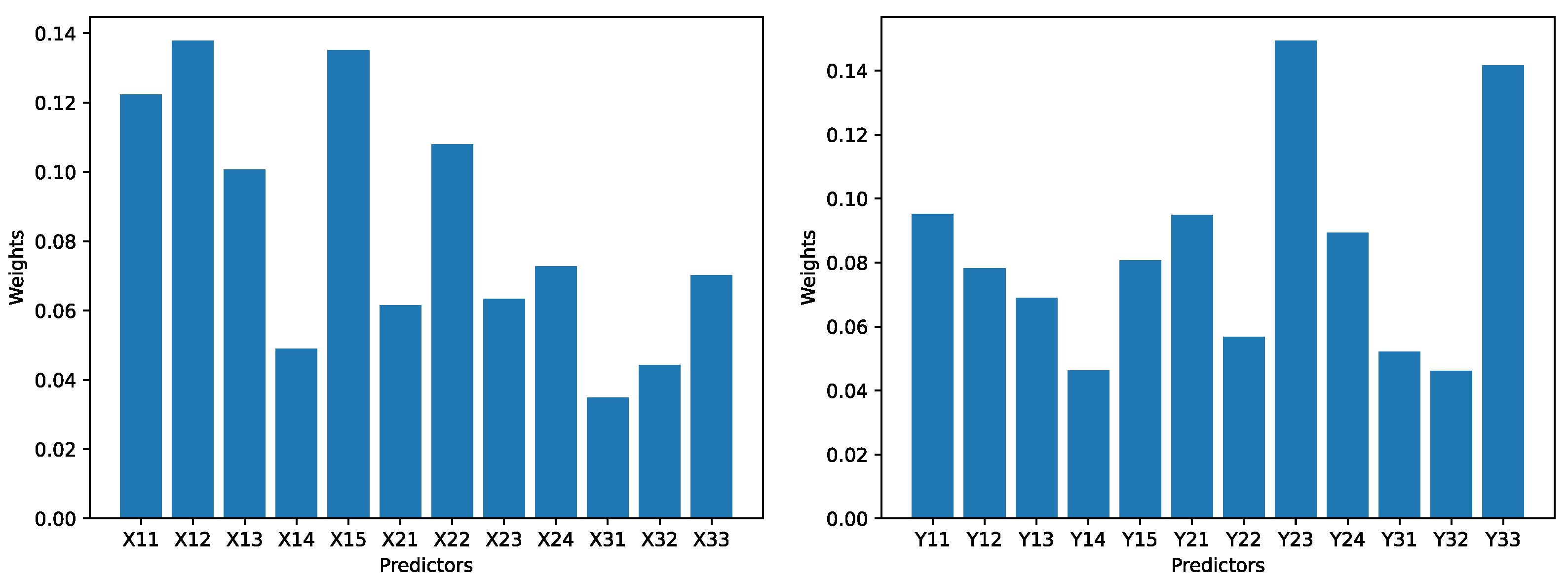

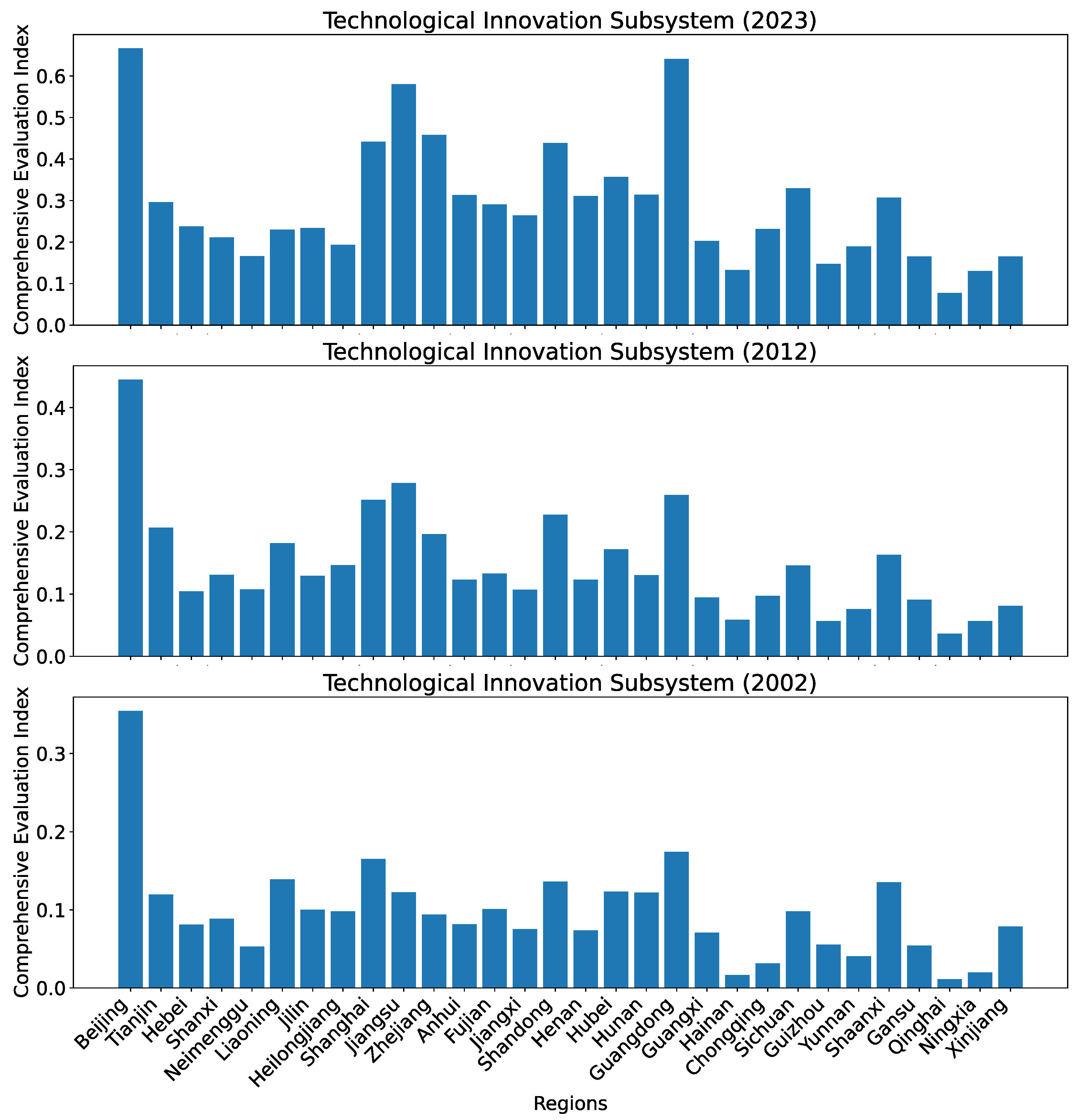

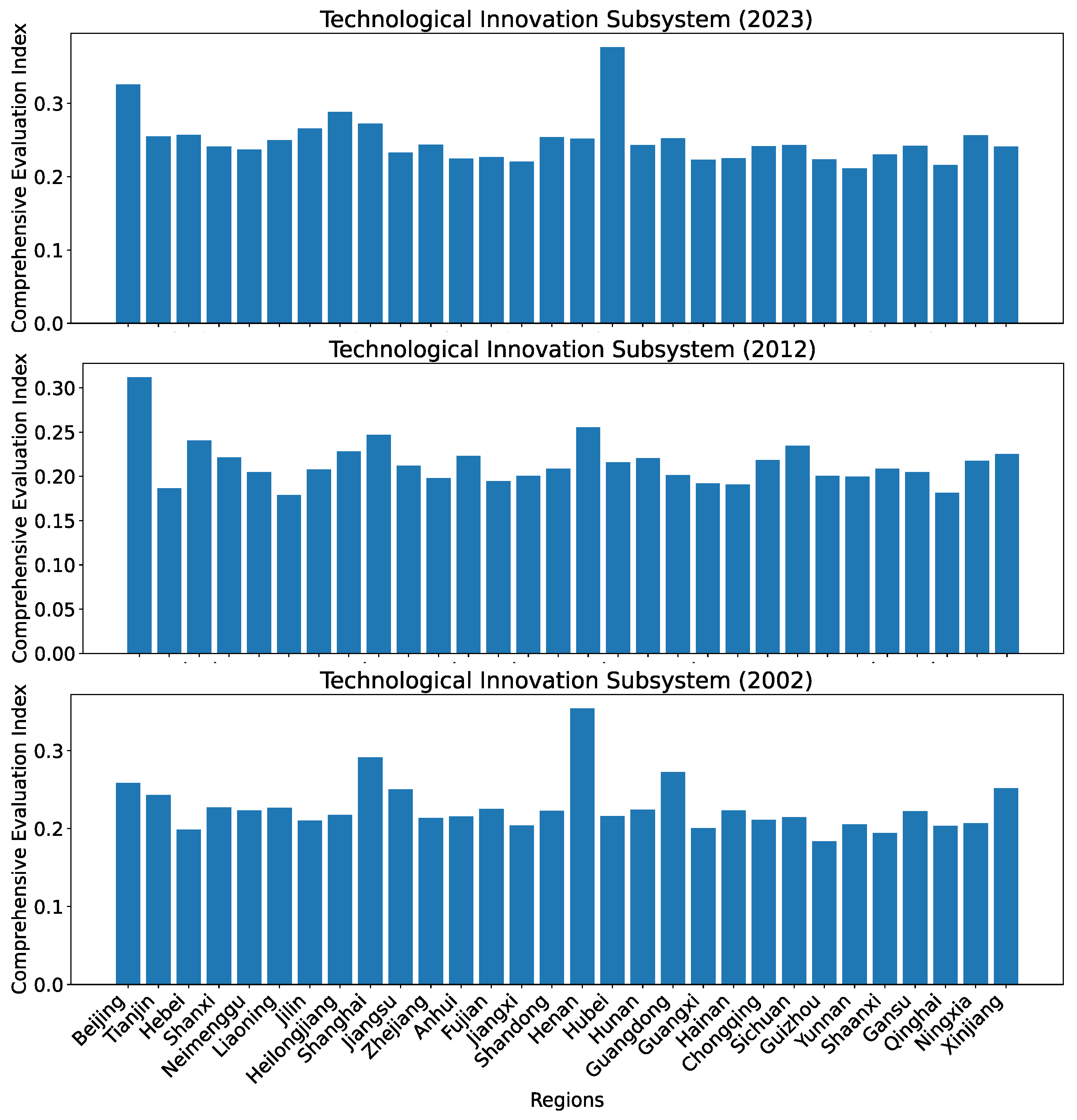
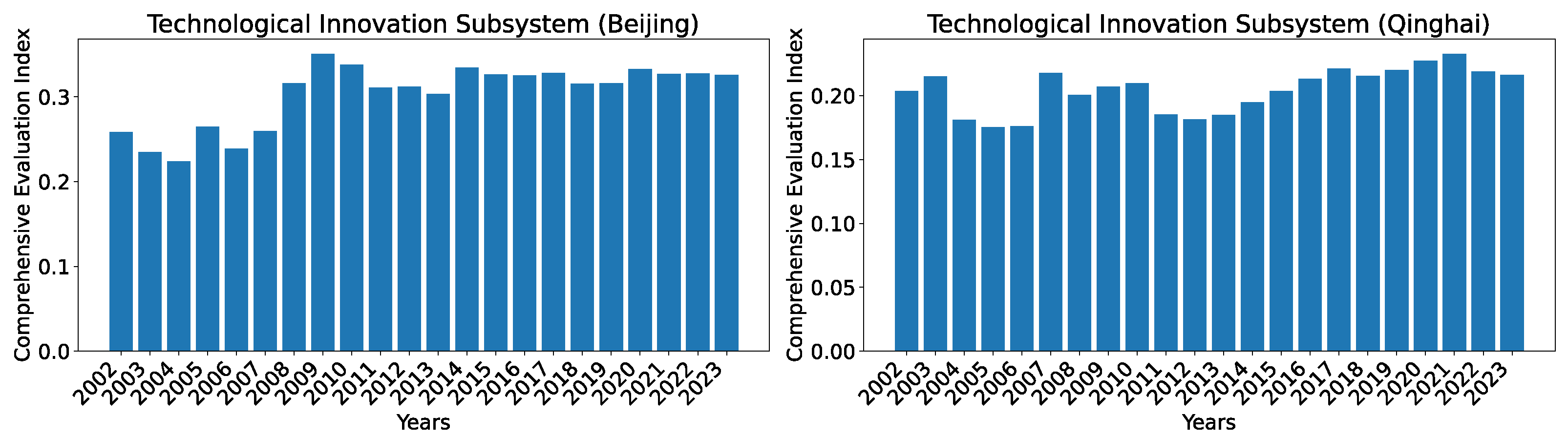


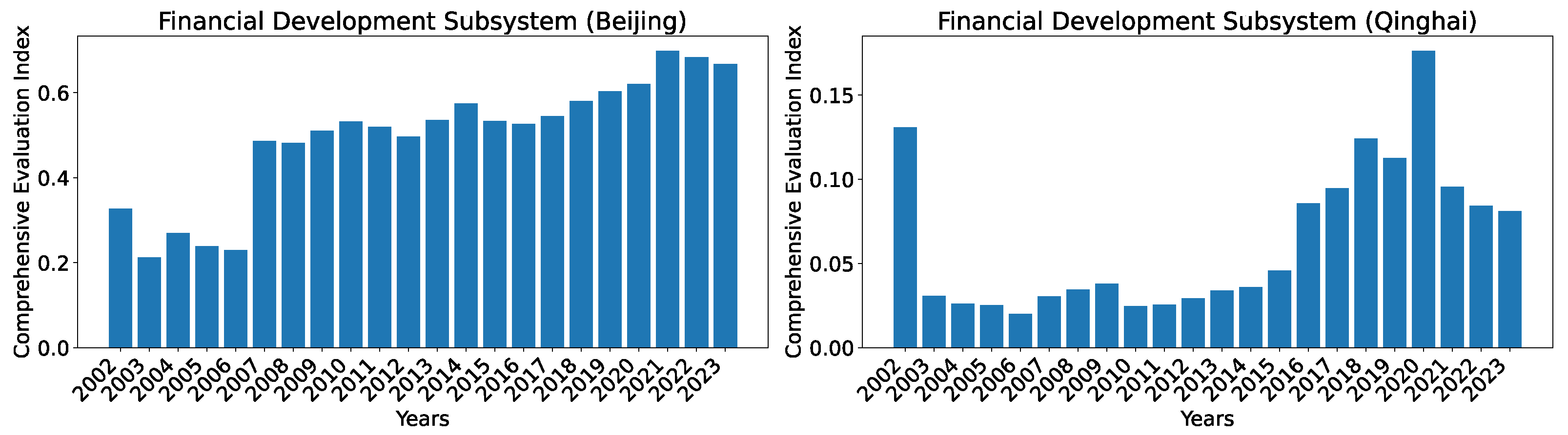
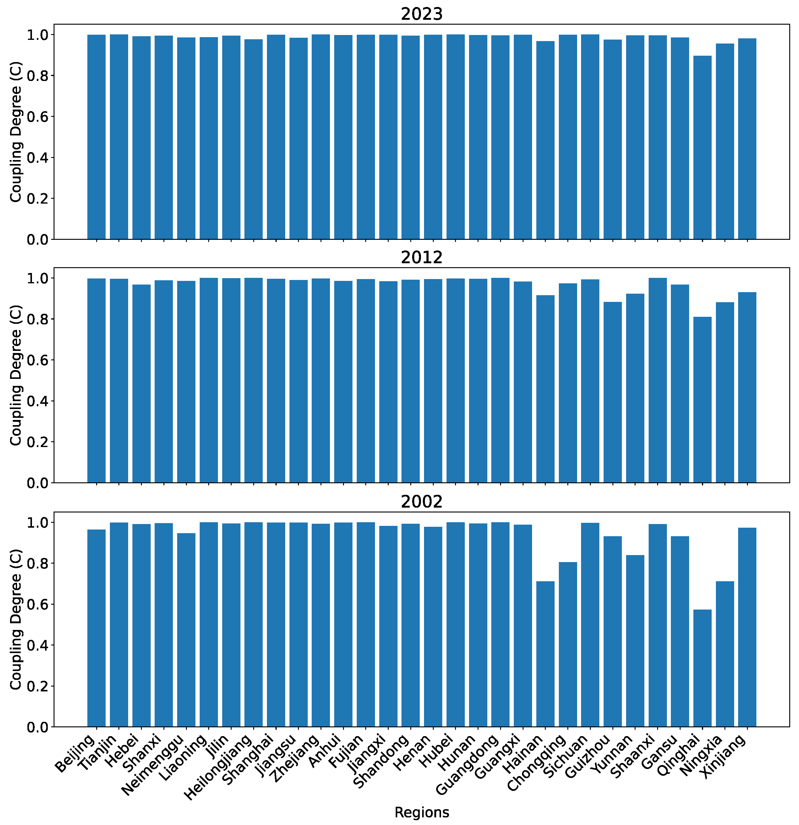


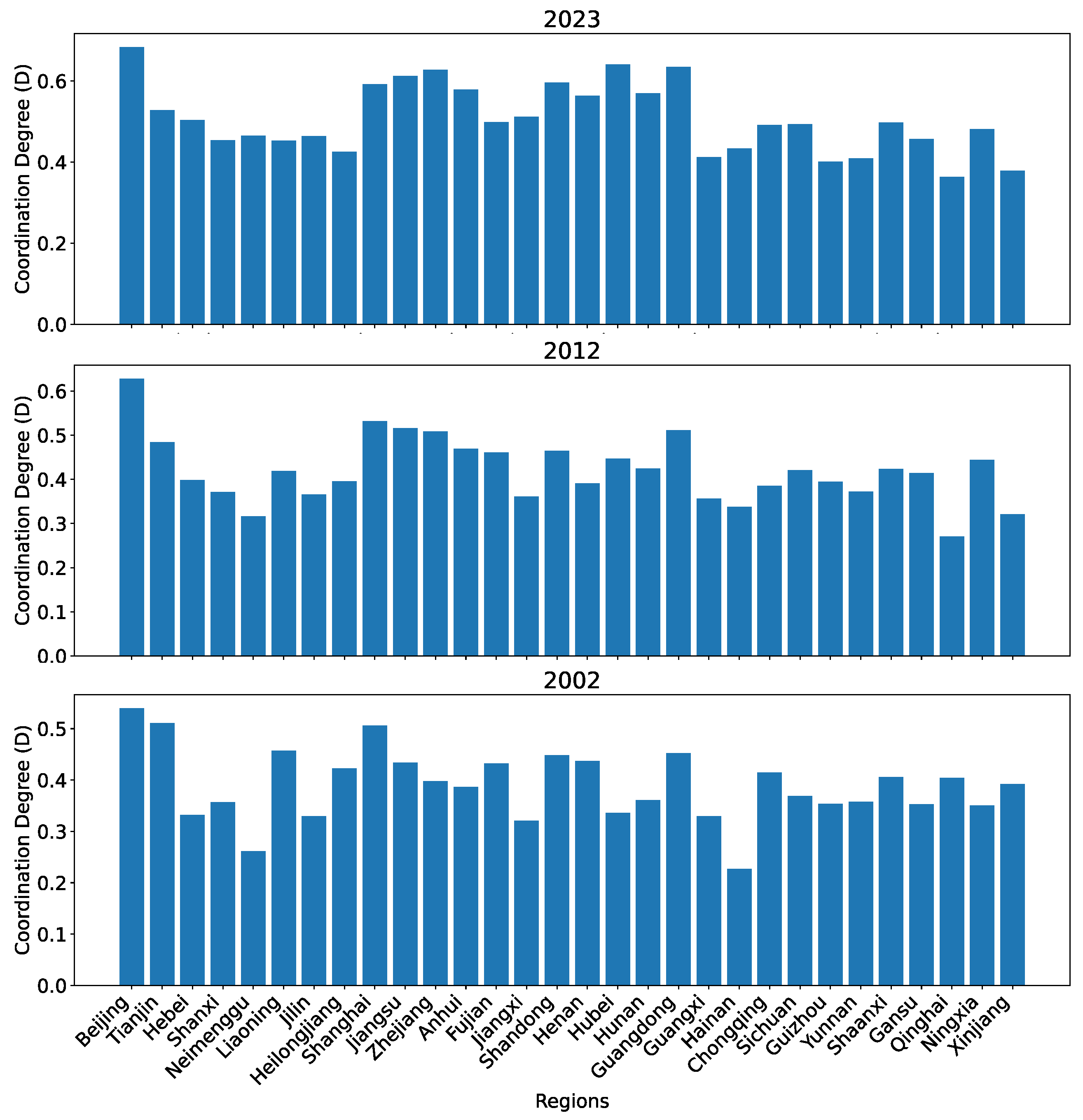


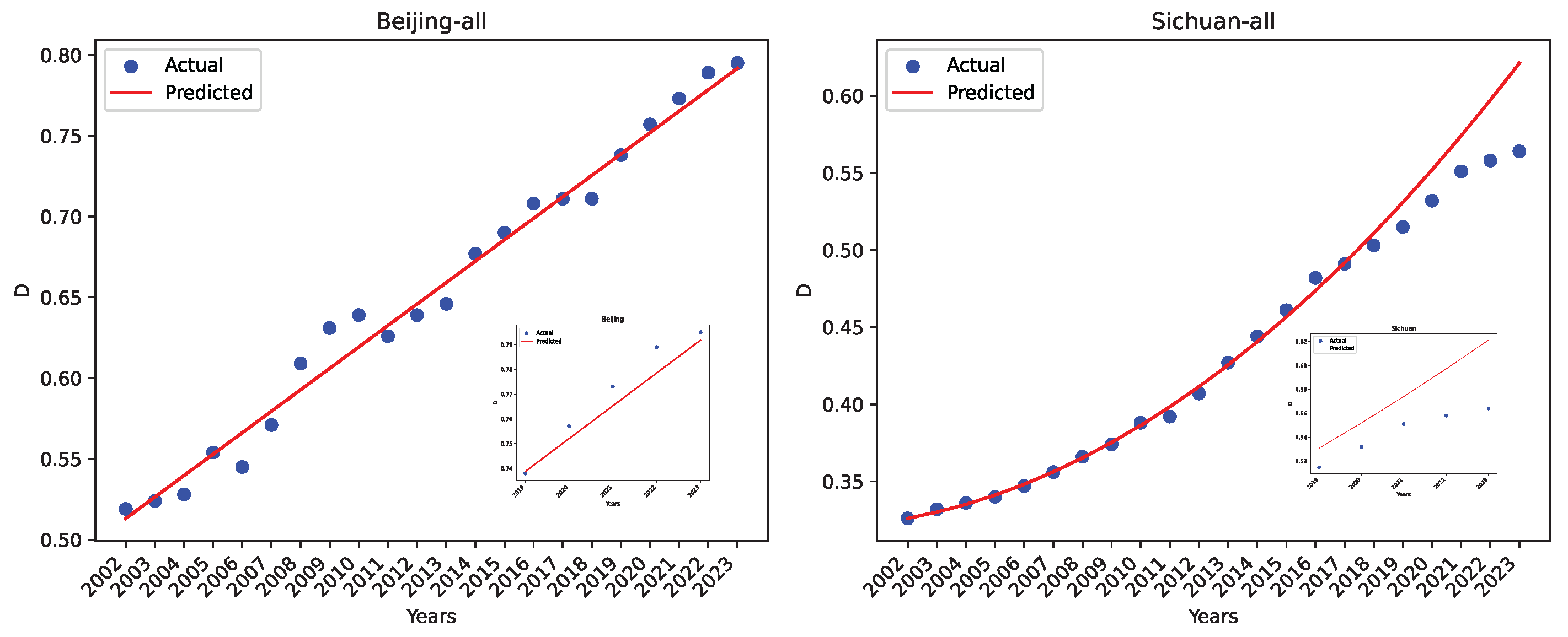


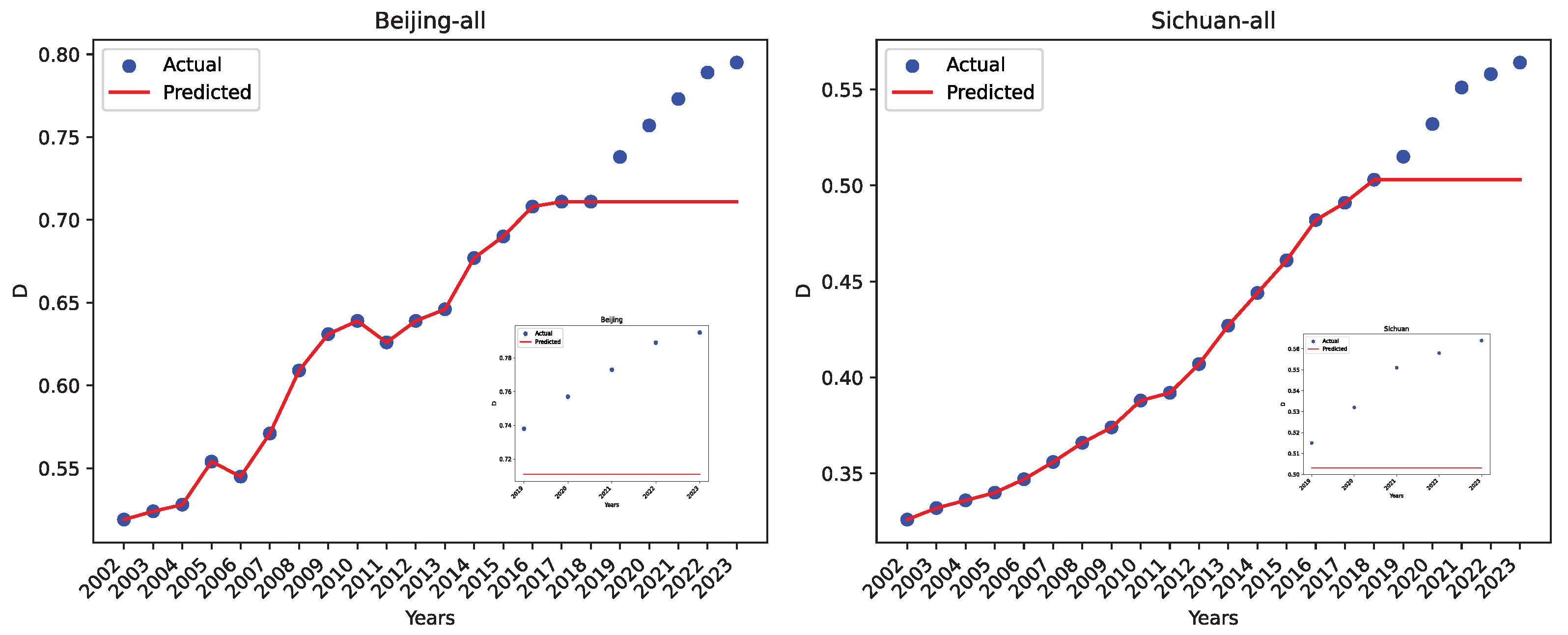
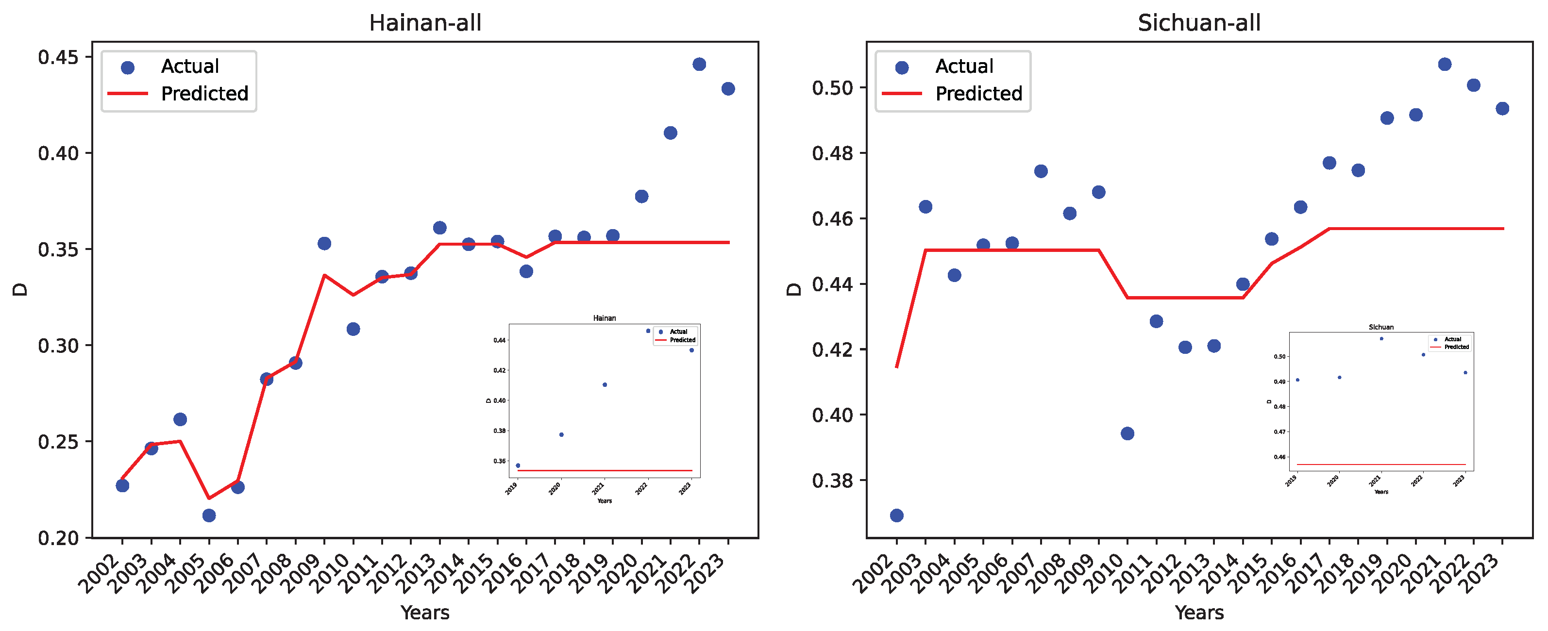

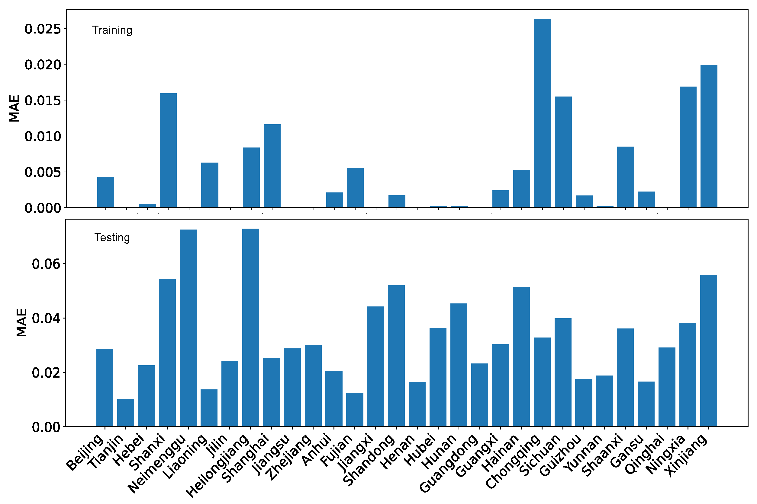


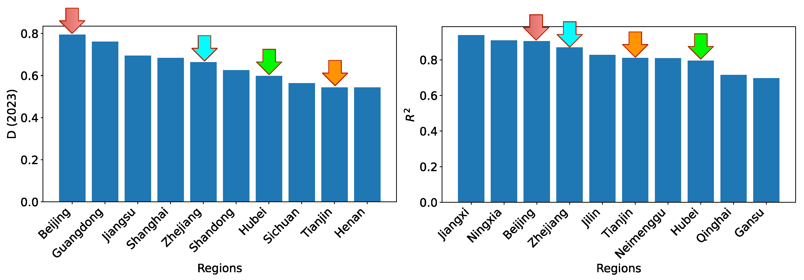
Disclaimer/Publisher’s Note: The statements, opinions and data contained in all publications are solely those of the individual author(s) and contributor(s) and not of MDPI and/or the editor(s). MDPI and/or the editor(s) disclaim responsibility for any injury to people or property resulting from any ideas, methods, instructions or products referred to in the content. |
© 2025 by the authors. Published by MDPI on behalf of the International Institute of Knowledge Innovation and Invention. Licensee MDPI, Basel, Switzerland. This article is an open access article distributed under the terms and conditions of the Creative Commons Attribution (CC BY) license (https://creativecommons.org/licenses/by/4.0/).