Microgrid Frequency Regulation Based on Precise Matching Between Power Commands and Load Consumption Using Shallow Neural Networks

Abstract

Islanded microgrids commonly use droop control methods for autonomous power distribution; however, this approach causes system frequency deviation when common loads change. This deviation can be eliminated using secondary control methods, but the core of this approach is to generate compensation values equal to the offset amount to add to the controller, thereby eliminating deviations from rated values. Such a mechanism can actually achieve the same effect by setting power reference values within the droop control method. The power references within the controller need to be adjusted dynamically, and they are associated with common load variations. Therefore, establishing a fitting relationship between the adjustment of power reference and changes in common loads can achieve better frequency regulation, keeping the system frequency operating within rated frequency ranges. These two types of data are correlated, however, due to physical parameters, the fitting between them is not strictly fixed in a mathematical sense. Thus, to find their interconnected relationships, using intelligent methods becomes crucial. This paper proposes a shallow neural network-based method to achieve fitting relationships. Moreover, to address power inputs with zero values, an input enhancement method is proposed to prevent potential gradient vanishing and ineffective learning problems. Thus, through precise matching between power commands and load consumption, the system frequency can be maintained near rated values. Various simulation scenarios demonstrate the feasibility and effectiveness of the proposed method.

1. Introduction

As a physical entity and operational unit, the microgrid is one of the components of virtual power plants (VPPs) [1]. Through the integration and optimization of distributed energy resources (DERs), VPPs rely on information technology and intelligent management to achieve virtual integration of dispersed resources through software and communication technologies, improving the flexibility and efficiency of their power systems. Microgrids can integrate distributed generations (DGs) through DERs for distributed power production and supply, along with loads, energy storage devices, power electronic converters, etc. For their operation and control, a hierarchical control approach is often adopted, where islanded microgrids can include a primary level covering droop control and a secondary level that corrects operational state deviations caused by droop control [2,3].

Currently, there are many studies investigating secondary control in microgrids. Secondary control can be classified into three types based on communication connection structure: centralized, distributed, and decentralized [4,5]. A secondary control method based on distributed model predictive control is proposed in [6] for frequency regulation in AC microgrids. A distributed control strategy is adopted in [7] and combined with a self-triggered mechanism for frequency restoration in AC microgrids. Reference [8] introduces a proportional-integral secondary control for frequency and voltage restoration in islanded microgrids. Reference [9] investigates improved secondary control strategies for dynamic boundary microgrids to enhance the resilience of distribution systems. A novel privacy-preserving average consensus algorithm is proposed in [10] to achieve distributed load sharing in microgrids.

However, these methods all aim to shift the droop characteristic curve by adding compensation to eliminate deviations caused by droop control. Frequency and voltage recovery is not achieved through load power adjustment. Yet, the same secondary control effect can actually be achieved by setting the power reference value in the droop control. However, this is from the perspective of power distribution at the primary level. For example, paper [11] proposed methods to eliminate operational state deviations, but the method used in that paper is achieved through quantitative numerical relationship corrections rather than using intelligent methods.

This paper draws on the same approach to correct operational state deviations, so the key is how to establish the proper numerical relationship between the power commands within the controller and the common load. Although these data sets maintain physical connectivity via power lines and impedance correlations, their numerical interdependence presents significant complexity due to the intricate control structure and circuit complexity.

To better explore the relationship between the abovementioned two data sets, artificial intelligence (AI) algorithms can be the preferred method due to their highly nonlinear mapping and self-learning capabilities. These have been successfully applied in power systems applications [12,13]. A shallow neural network (SNN) reward model is used in [14] to control grid-connected microgrids. The SNN is adopted in [15] for short-term hourly energy consumption prediction. Reference [16] explores the potential of AI-based solutions for hierarchical control layers and investigates AI-driven strategies for single and networked microgrid environments. Reference [17] utilizes deep reinforcement learning to develop a resilience-oriented microgrid formation method for distribution networks. A two-stage deep learning approach is proposed in [18] to solve the economic dispatch problem in microgrids. A summary of the above literature review is shown in

Table 1. Comparison of the proposed methods with existing techniques in the literature.

Reference	Offset Elimination Level		Artificial Intelligence Methods Employed
	Primary	Secondary	SNN	DNN	ANN (No Clarity Whether It Is Shallow or Deep)
[6]	✗	✓	✗	✗	-
[7]	✗	✓	✗	✗	-
[8]	✗	✓	✗	✗	-
[9]	✗	✓	✗	✗	-
[11]	✓	✗	-	-	✓ but for load power forecasting
[12]	-	-	-	-	✓
[13]	-	-	✓	✓	-
[14]	-	-	✓	✗	-
[15]	-	-	✓	✗	-
[17]	-	-	✗	✓	-
[18]	-	-	✗	✓	-

. In the table, ✓ indicates “involved”, ✗ indicates “not involved”, and - indicates “no content in this aspect”.

Taking artificial neural networks (ANNs) as an example in terms of network architecture complexity and depth, these implementations can be categorized into two primary frameworks: deep neural networks (DNNs) and SNNs [19,20]. When comparing DNNs and SNNs, it becomes apparent that DNNs have more complex network structures with more hidden layers and neurons. This means they require larger amounts of data and longer training and evaluation periods to obtain highly satisfactory models suitable for control applications. Given the real-time requirements of control systems, the SNN model becomes very convenient and simple, provided it meets data-fitting accuracy requirements [21,22,23]. Compared to DNNs, SNNs contain fewer parameters and provide higher training efficiency with immediate feedback and quick adjustments. SNNs require significantly fewer computational resources during both training and inference. This efficiency makes them particularly suitable for microgrid control applications that demand rapid response in real-time systems. SNNs demonstrate superior generalization on small datasets while reducing overfitting risks and are easier to tune and optimize. These characteristics make SNNs more robust for small- to medium-sized datasets. Their simpler structure also makes their behavior more transparent and easier to analyze, while providing more stable performance when input conditions vary.

Leveraging the aforementioned advantages of SNNs and approach of setting power commands at the primary level, this paper will conduct frequency regulation for AC microgrid systems and fully explore the degree and potential of precise matching between power commands and load consumption. This paper makes the following key contributions:

• Unlike previous research, which typically defaults power reference values to zero, this paper conducts a comprehensive analysis of optimal power reference value configurations in droop control. A direct relationship is established between the power variations of time-varying public loads and the power reference values in droop control within the controller, leading to enhanced system frequency stability and offset correction.
• Unlike paper [11], which uses quantitative numerical relationship corrections to eliminate operational state deviations, this study’s SNNs are designed to match power commands with load consumption to deliver efficient and accurate results. Moreover, an input enhancement method is proposed to mitigate gradient vanishing and enhance SNN stability when addressing power inputs with zero values.
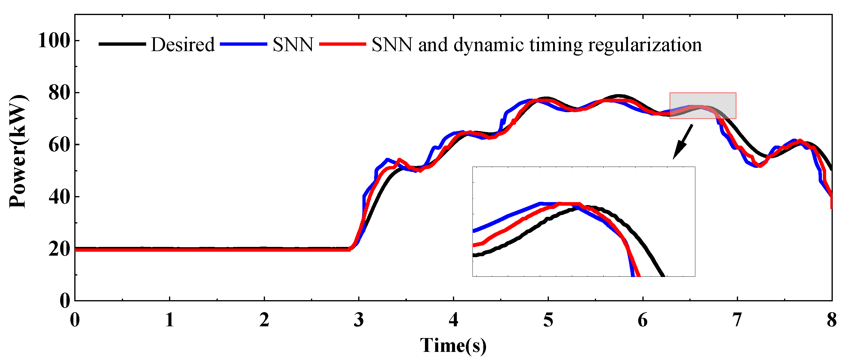
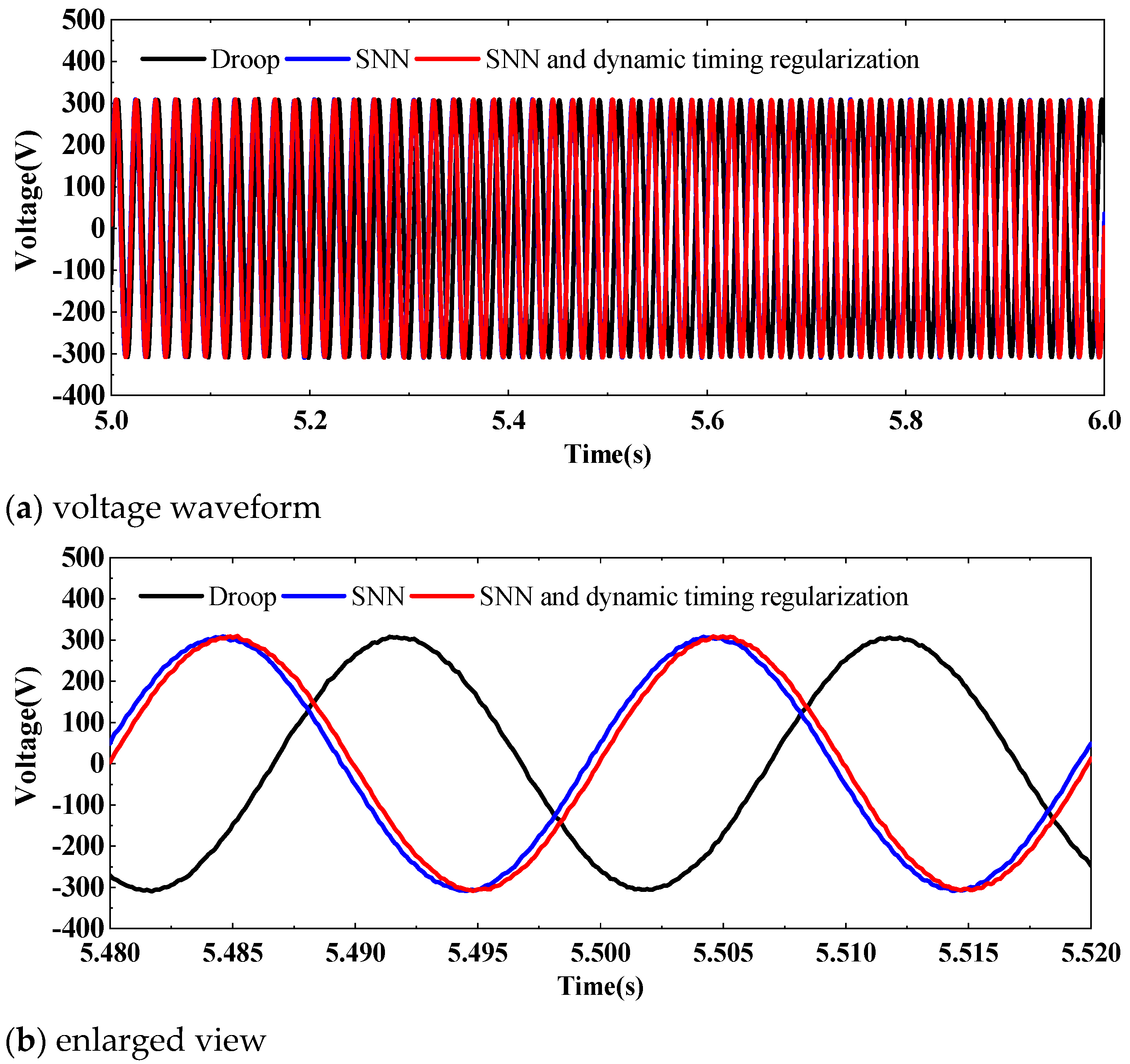
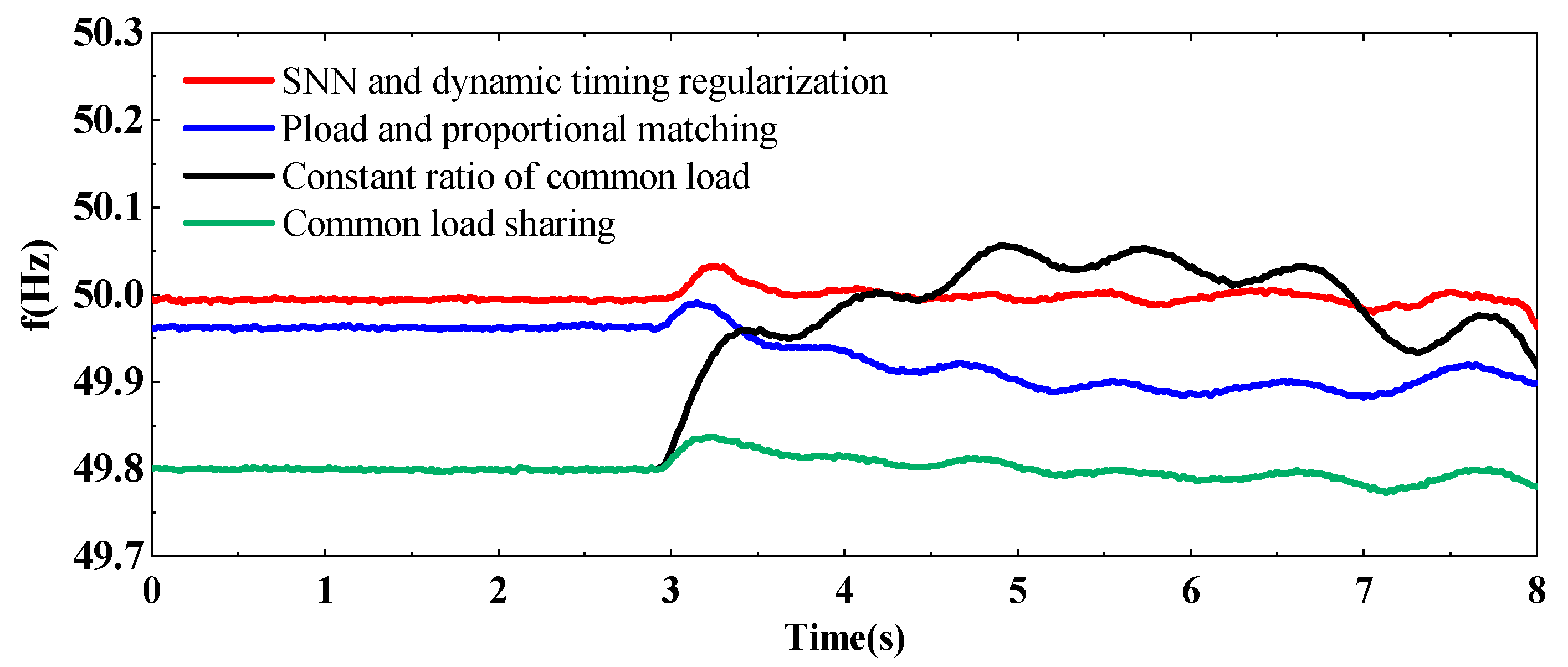
• To further correct the time delay and data misalignment issues between curves caused by SNN fitting, a dynamic timing regularization is proposed to achieve precise peak-to-peak correspondence between curves. As a result, frequency regulation becomes more stable at the rated value.

Figure 1 illustrates the AC microgrid topology implemented in this paper. AC microgrids are currently the predominant type and can operate in islanded mode when disconnected from the main grid via an electrical switch. The DGs can be connected in parallel to the AC bus through transmission lines. The system frequency, which primarily refers to the AC bus frequency, must be unified to ensure equipment synchronization and a stable power supply.

This paper is organized into five sections. Section 2 describes the basic hierarchical control and power commands used for system frequency regulation. Section 3 presents the proposed methodology, including data preparation and processing for SNN training, SNN configuration, and the matching process. Section 4 presents and analyzes the simulation results. Section 5 summarizes the paper’s conclusions.

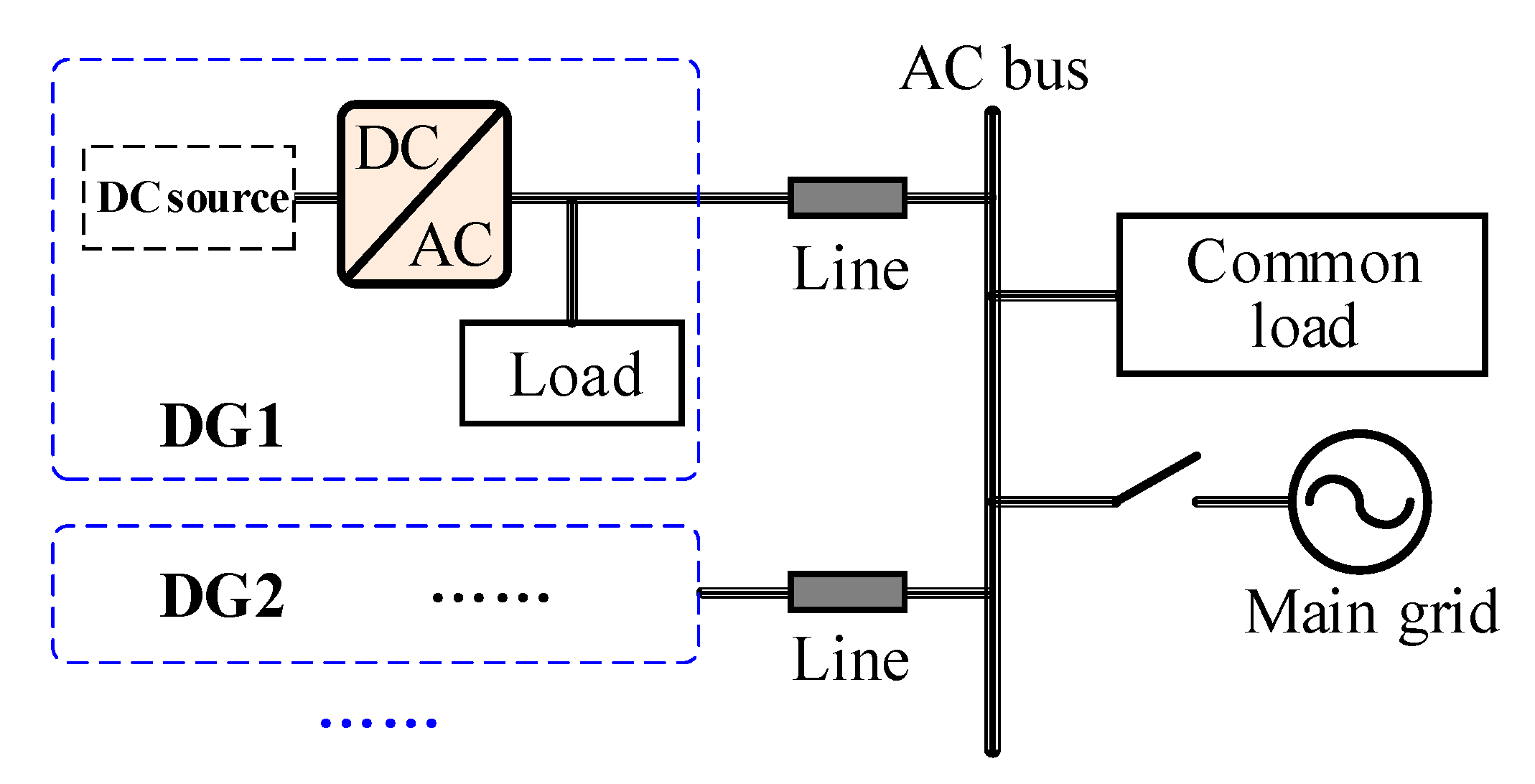
2. Hierarchical Control for Frequency Regulation

2.1. Primary Level

The primary level maintains local control stability and manages power converter drive signals. Regarding autonomous power distribution, as mentioned earlier, droop control is a common method for parallel AC interface DGs. To achieve the desired AC frequency amplitude ω, the system compares the measured active power value P with the reference values P* through the droop equation below [24]:

$$\omega ={\omega }^{*}-m(P-P^{*})$$

(1)

where ω* represents the rated value of ω and m is the droop slope.

The calculation of m is determined by

$$m=\Delta \omega /P_{max}$$

(2)

where Δω represents the maximum frequency deviation limit, while P_max denotes the maximum inverter output active power.

In much of the existing literature, this power reference value P* is typically set to zero to simplify control logic and adapt to various operating modes. The droop control is simplified to use frequency as a feedback signal to automatically adjust the power output of the DG, thereby ensuring system stability.

2.2. Secondary Level

From the above droop control formula, it is evident that when P* maintains a constant value and both P and the coefficient m are positive, when P and P* are not equal, ω will not equal the rated value ω*, resulting in a frequency deviation. To address these deviations, the secondary level employs compensation δω to adjust and normalize the value to its rated value. This adjustment is executed through the following formulas, utilizing a PI controller as the general method [25,26]:

$$\omega ={\omega }^{*}-mP+\delta \omega$$

(3)

$$\delta \omega =K_{p\omega } \left({\omega }^{*}-\omega \right)+K_{i\omega }{\displaystyle \int \left({\omega }^{*}-\omega \right) dt}$$

(4)

where K_pω and K_iω are PI control coefficients.

However, this implementation of the secondary level is achieved by generating additional compensation. That is, through the PI controller, the offset caused by the primary level is restored to the rated value through quantitative addition.

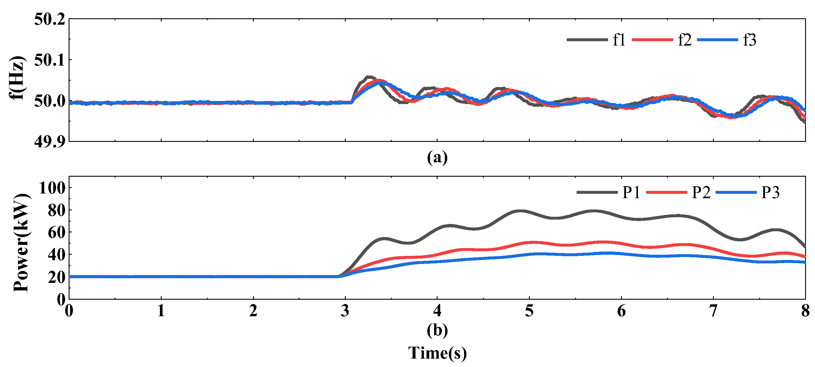
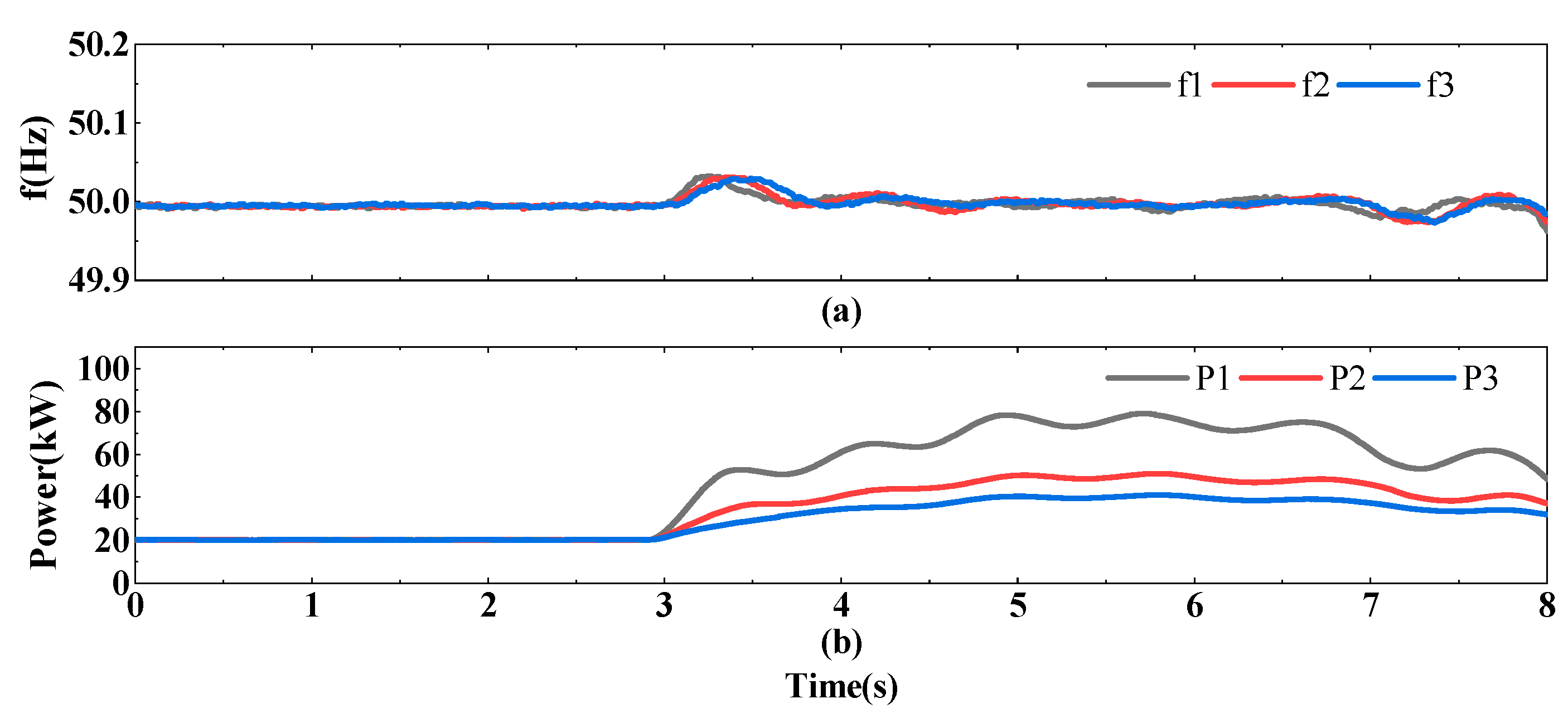
2.3. Frequency Regulation

As mentioned above, to achieve a secondary level effect while maintaining the primary level foundation, Formula (5) can be derived by comparing Formulas (1) and (3), where the corresponding relationship reveals the specific components that implement the secondary compensation.

$$m{P}^{*}=\delta \omega$$

(5)

In other words, looking at the droop control formula alone, if the power reference value can be treated as a manipulable variable, its product with the droop coefficient actually represents the secondary control compensation amount.

Returning to Formula (1) of droop control, maintaining the system’s real-time frequency at its rated value requires an equation like Formula (6). After simplification, an analysis concludes that the power reference value P* must equal the DG’s output power P, as demonstrated in Formula (7). This output power is configured within the controller.

$$\omega ={\omega }^{*}-m(P-P^{*})={\omega }^{*}$$

(6)

$$P^{*}=P$$

(7)

Therefore, the next key task is implementing Formula (7). The DG’s power output primarily depends on two types of loads: local and common. Local loads, situated near the DG controller, have easily measurable power levels. Common loads, however, are typically located farther away, making their power levels harder to monitor in real time. Furthermore, DGs are classified as either dispatchable or non-dispatchable based on their load type. This study focuses on dispatchable DGs, which can adjust their power output to track accurate load prediction values used as setpoints. The approach can also generalize to other microgrid topologies or systems with different line impedances, DG capacities, or load types. These require modifications to SNN model training and dynamic timing regularization to update the power reference values in the controller.

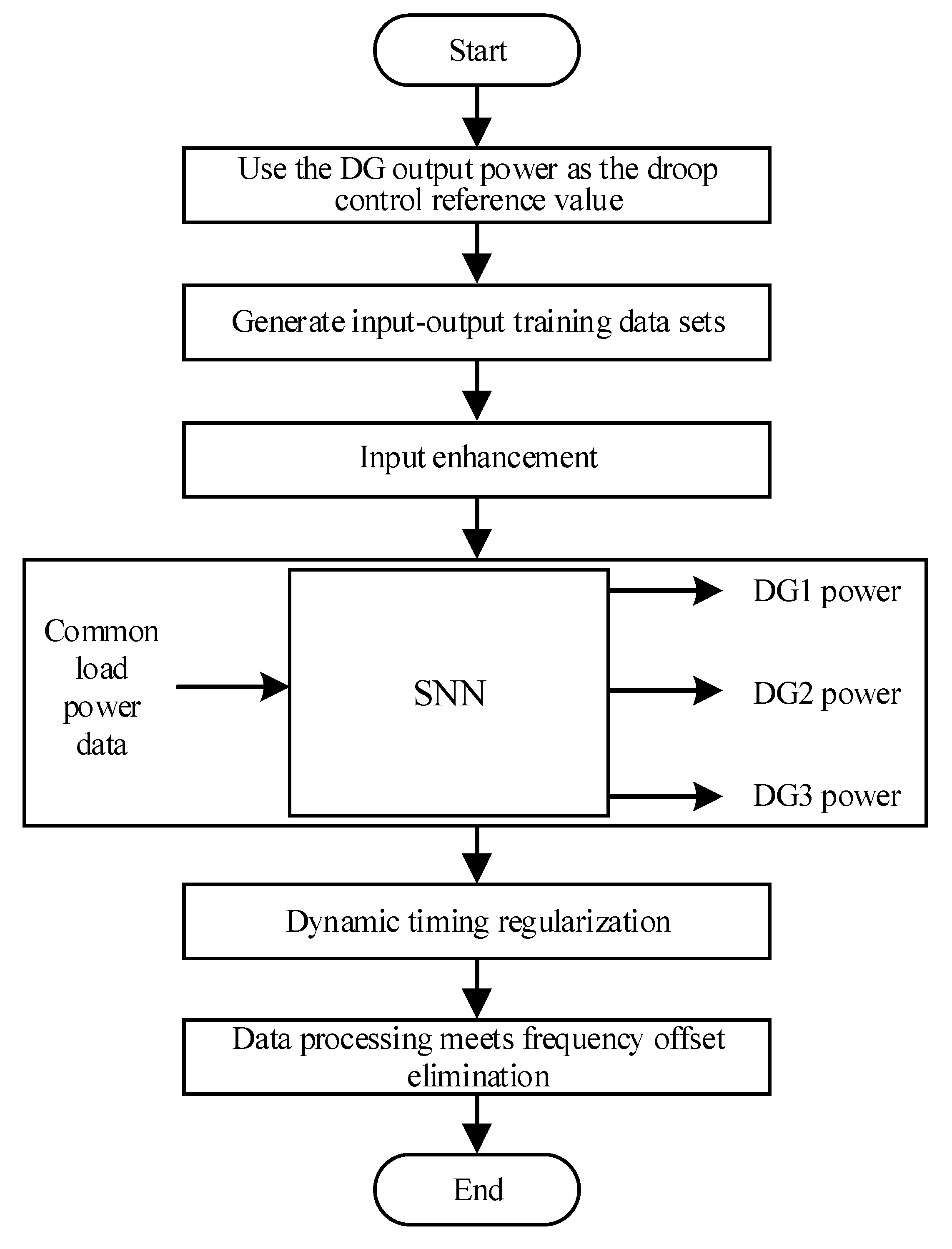
3. Proposed Control Methods

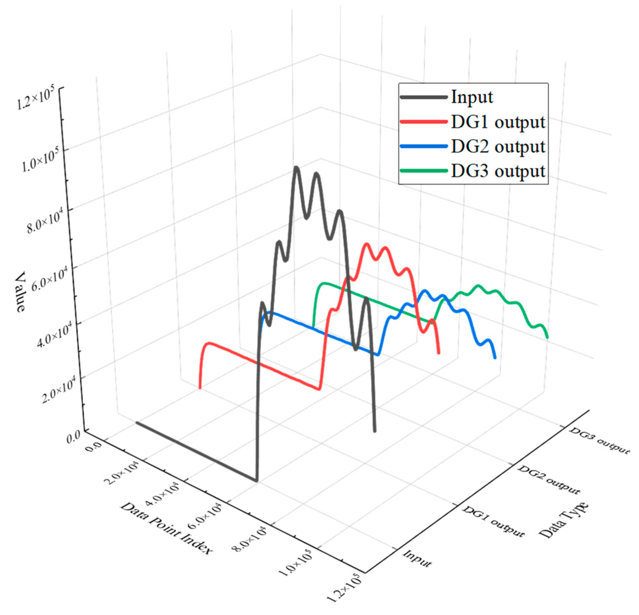
3.1. Data Preparation and Processing

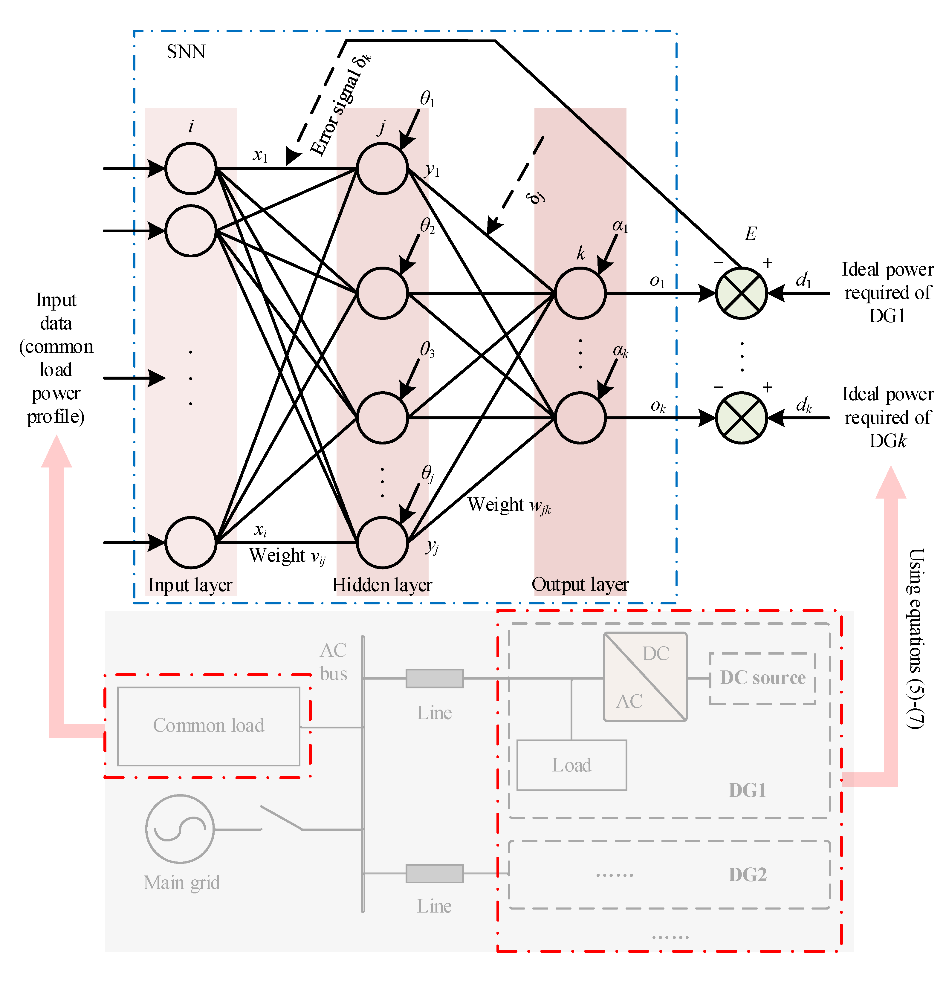
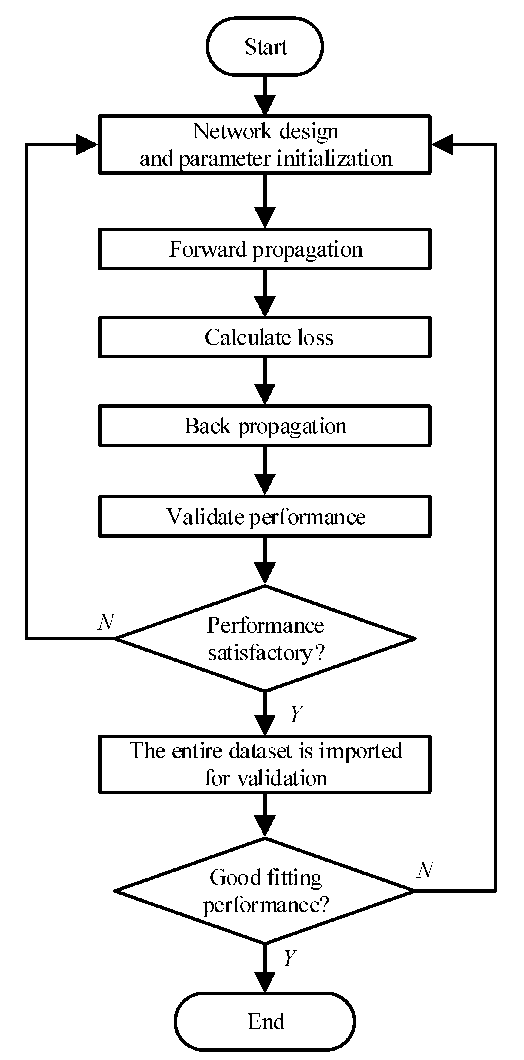
The first step is to clarify the available data and required preparation and processing. One is power commands in the controller, and the other is load changes in the system. Since the DG output varies with load changes, the main task is to establish the power commands settings based on load consumption, especially from common loads. The data-matching process needs to build relationship between power commands and load consumption. Load consumption therefore serves as input data, while power commands become output data. Thus, the system’s load consumption changes can be converted into corresponding power commands within the controller.

So where does this data come from? Thanks to the smart meters, phasor measurement units, and supervisory control and data acquisition systems equipped during the intelligent construction of microgrids, the power consumption of loads and output power of DGs can be measured and recorded in real time. This is sufficient to support the source of the aforementioned power data. Among these, the common load power variations, which serve as input data, are provided by the above systems and can be obtained even when the microgrid is operating only at the primary level. The key questions are how much controller input power each DG actually needs, and how to obtain this through the already-known common load power variations.

Based on these secondary-level control principles, the PI controller can compensate for the offset introduced by droop control at the primary level, providing insights into setting the controller input powers. Under this secondary level scenario, when the system operates stably, input and output data are collected for artificial intelligence neural network algorithm training. The collection results are shown in the Figure 2. The first black curve represents the common load power as training input, while the second to fourth (red, blue, and green) curves represent the required controller input powers for DG1 to DG3, respectively, as training outputs.

To maintain data collection correspondence and ensure sufficient training data volume, a sample-and-hold circuit is employed. Its function is to capture the input signal value at each sampling moment and maintain this value unchanged until the next sampling moment, with relatively short intervals between sampling moments. This is implemented through the following formula:

$$y(t)=u(kT)\mathrm{for}kT\le t\le (k+1)T$$

(8)

where T is the sampling period, which is set to 1 × 10⁻⁴ s in this study, u(kT) is the value of the input signal at sampling instant kT, and y(t) is the output signal.

Based on the above discussion, it can be deduced that the power reference value P* can be calculated using the following formula, noting that the system maintains a stable operating state, ignoring transient fluctuations and oscillations:

$$P^{*}={\displaystyle \frac{1}{m}}\delta \omega ={\displaystyle \frac{1}{m}}\left(K_{p\omega } \left({\omega }^{*}-\omega \right)+K_{i\omega }{\displaystyle \int \left({\omega }^{*}-\omega \right) dt}\right)$$

(9)

Through the above formula, when there are changes in common load power, by correcting the real-time system frequency through the secondary level, the P* value for each DG can be obtained, thereby achieving frequency restoration to the rated value at the primary level without using the secondary level.

Here, the data provided for subsequent neural network training can only be obtained initially through the secondary level control compensator. However, through one-shot or few-shot learning, the system can still be prepared for generalization and control at the primary level. The main reason is that microgrids operate within a specified frequency range bounded by upper and lower limits. The maximum frequency fluctuations are typically restricted to ±0.8 Hz or ±0.5 Hz, though these specific limits vary by country and region. Therefore, by traversing the relationship between frequency variations within this range and common load power changes, the fitting model can achieve good generalization capabilities.

3.2. SNN

SNNs are an important algorithm in the field of machine learning, which uses mathematical modeling techniques to build versatile approximators. These networks effectively model and predict intricate data relationships while approximating complex functional relationships in a highly non-linear manner. SNNs primarily consist of a single hidden layer architecture with an input layer and an output layer. According to the method of learning connection weights, SNNs follow the universal learning process of neural networks and can be categorized into two types: those utilizing backward learning (BL) approaches and those implementing forward learning (FL) methodologies.

As previously mentioned, SNNs have fewer parameters, simpler structure, fewer hidden layers, and lower overfitting risk than DNNs. The main characteristic that distinguishes SNNs from DNNs is their fewer number of hidden layers and relatively simpler structure. However, SNNs still follow the backpropagation (BP) training mechanism, maintaining consistency with DNNs and traditional BP neural networks in terms of basic structure and training principles. The basic structure and theoretical expressions of SNNs used in this paper are described below.

In Figure 3, each of the three layers (input, hidden, and output) contains n, m, and l neurons respectively. The network’s output vectors comprise x_i (i = 1, 2, …, n) in the input layer, y_j (j = 1, 2, …, m) in the hidden layer, and o_k (k = 1, 2, …, l) in the output layer, with d_k denoting the target output. The interconnections between layers are characterized by neuron weights v_ij and w_jk, while the output and hidden layers utilize thresholds α_k and θ_j, respectively.

The following equation applies to the hidden layer:

$$y_j=f(ne{t}_j)=f({\displaystyle \sum _{i=1}^n{v}_{ij}{x}_i})$$

(10)

For the output layer, the equation is as follows:

$$o_k=f(ne{t}_k)=f({\displaystyle \sum _{j=1}^m{w}_{jk}{y}_j})$$

(11)

Within these equations, the unipolar Sigmoid function is employed as the transformation function f(x):

$$f(x)=1/(1+e^{-x})$$

(12)

When the network output O differs from the expected output D, an output error E is defined as follows:

$$\mathit{E}={\displaystyle \frac{1}{2}}{(\mathit{D}-\mathit{O})}^2={\displaystyle \frac{1}{2}}{\displaystyle \sum _{k=1}^l{(d_k-o_k)}^2}={\displaystyle \frac{1}{2}}{\displaystyle \sum _{k=1}^l{[d_k-f({\displaystyle \sum _{j=1}^m{w}_{jk}{y}_j})]}^2}$$

(13)

The output error E can also be expanded further into the hidden layer:

$$\mathit{E}={\displaystyle \frac{1}{2}}{\displaystyle \sum _{k=1}^l{\{d_k-f[{\displaystyle \sum _{j=1}^m{w}_{jk}f({\displaystyle \sum _{i=1}^n{v}_{ij}{x}_i)}}]\}}^2}$$

(14)

Since SNNs use the standard BP training mechanism to adjust their learning rate, weights, and thresholds, this part will not be elaborated further.

Neural network training follows a systematic process that begins with data preparation and network design. After parameter initialization, the network uses forward propagation to generate predictions. A loss function measures the difference between predictions and actual values, while the backpropagation algorithm updates network parameters. This process repeats until performance reaches a satisfactory level, with an independent test set verifying the model’s ability to generalize. Based on validation results, the network structure and hyperparameters are then fine-tuned to enhance overall performance. The flowchart for SNN fitting is shown in Figure 4.

Here, data fitting with SNNs is a critical core step, but a challenge remains. That challenge is the time series nature of the data, specifically, whether a one-to-one correspondence exists between data points for control systems. The requirements for this real-time nature and the degree of matching between them are relatively high. Next, further data processing will be conducted to achieve high-precision predictive control.

With regard to the microgrid control implementation, SNNs offer a lightweight yet effective solution for real-time control. They efficiently manage voltage, frequency, and load dynamics through their simple design and rapid processing capabilities. These attributes make them particularly suitable for deployment on resource-constrained edge devices, where rapid decision-making is critical. Moreover, SNNs enhance microgrid reliability by enabling real-time fault detection and improving stability during islanded operation. However, their ability to handle highly nonlinear, complex, or time-dependent microgrid dynamics remains limited, as they lack the depth required to model intricate system behaviors accurately. To ensure robust performance, SNNs depend heavily on high-quality training data, necessitating careful data collection, preprocessing, and feature engineering to mitigate biases and improve generalization. Proper dataset selection, noise reduction techniques, and balanced representation of operational scenarios are essential steps to maximize their effectiveness in real-world microgrid applications.

3.3. Power Matching

From the data curve that needs to be fitted in Figure 2, there are sinusoidal-like peak and valley fluctuations between the input and output data. After the neural network completes data prediction, the forecasted and actual peaks cannot be perfectly aligned, but will have a time delay, which is undesirable for frequency regulation. The next step involves matching data by adjusting each DG’s forecasted power to align with the ideal power required for eliminating frequency deviation, primarily focusing on timing regularization. While previous research has employed experience-based amplitude adjustments and delay compensation, these approaches lack dynamic adaptability. This paper will instead use a dynamic timing regularization method.

Dynamic timing regularization processes time series data of varying lengths [27,28]. The core concept involves finding an alignment or regularization path that minimizes the cumulative sum of distances between corresponding points in two time series. This enables the identification and matching of similar features, such as peaks, within the time series.

The first step calculates a distance matrix between two input time series. Each matrix element represents the distance between corresponding points in the sequences, typically measured using Euclidean distance. This quantifies the cost of each possible point-to-point matching between power commands and load consumption, providing a global perspective for preliminary assessment.

Next, a dynamic programming algorithm is applied to determine the path with the lowest cumulative cost, i.e., the regularization path. This path shows how points in one sequence optimally correspond to points in another while minimizing the overall distance metric. The process may involve non-linear stretching or compression to compensate for slight shifts along the time axis. Constraints can be added to speed up computation or enforce local alignment. The method outputs both a cumulative distance value and the regularization path, showing which points align with each other. This is especially useful for identifying time series with similar peak patterns. The following key steps complete the process described above:

First, construct distance matrix D, where D_i,j represents the distance between the ith point in sequence X and the jth point in sequence Y. The Euclidean distance is typically used:

$$D_{i,j}=d(x_i,y_j)=\sqrt{{(x_i-y_j)}^2}$$

(15)

Next, define a cumulative distance matrix C, where C_i,j represents the minimum cumulative distance from the starting point to point (i, j). Its recursive definition is as follows:

$$C_{i,j}=D_{i,j}+\min (C_{i-1,j},C_{i,j-1},C_{i-1,j-1})$$

(16)

where C_0,0 = 0, and for all cases where i > 0 or j > 0, C_i,0 = ∞ and C_0,j = ∞ (except for C_0,0), thus ensuring the path starts from the origin.

Finally, determine the optimal warping path P = {(p₁,q₁), (p₂,q₂), …, (p_k,q_k)} that minimizes the cumulative distance C_n,m, where the path has a starting point at (0, 0) and an endpoint at (n, m). Each step can move vertically, horizontally, or diagonally. Skipping samples or repeating signal features is not allowed, ensuring each point in the sequences is visited at least once.

As shown in Figure 2, anomalies in weight updates may be created during network training when the input data is 0 but the output data is a large non-zero value. In such cases, under the influence of the activation function, gradient vanishing issues are likely to occur. Conversely, if the network attempts to quickly adjust to generate larger output values, this may lead to gradient explosion. Furthermore, input data of 0 may prevent the network from learning effective feature representations due to insufficient information to distinguish between different inputs. At the same time, the error calculated by the loss function may become very large, making the optimization process unstable and difficult to converge.

This paper proposes an input enhancement method to address these issues. During the training process, this method demonstrated both faster training speeds and more stable model performance. This method replaces zero input data with known target output data after minor scaling, thereby avoiding the numerous problems mentioned above.

There is an input data vector x containing many zero-value elements and a target output data vector y. The aim is to replace the zero values in x with scaled-down values. Let the scaling value be α, where 0 < α ≪y (meaning it is a small constant much less than target data). Then, this method can be expressed as:

$${x_i}^{\prime }=\left\{\begin{array}{c}{x}_i,\mathrm{if}{x}_i\ne 0\\ \alpha ,\mathrm{if}{x}_i=0\end{array}\right.$$

(17)

where, x_i′ is the i-th element of the updated input data vector x′. If the original input data x_i is not 0, it remains unchanged; if it is 0, it is replaced by the target output data y_i multiplied by a small scaling coefficient α. It should be noted here that if the value of α is too large, it will affect training accuracy. Setting a small, non-zero value only serves to avoid issues such as anomalies in weight updates to some extent. In our work, the choice of α was primarily guided by empirical observations and iterative experimentation through extensive trial-and-error.

The complete data processing flow is illustrated in the Figure 5. After these steps are completed, frequency regulation can be performed. As shown in Figure 5, the data processing workflow involves several key steps. The process begins by using each DG’s output power as the power reference value input for the droop controller and collecting input-output datasets from frequency deviation elimination scenarios in secondary control. Data enhancement processing is then applied to address zero-value inputs in the training dataset. After the construction of an SNN model and completion of network training, dynamic timing regularization is performed to align data points more precisely, which improves prediction accuracy. This approach enhances both frequency elimination and frequency deviation correction. Finally, the entire data processing workflow is completed.

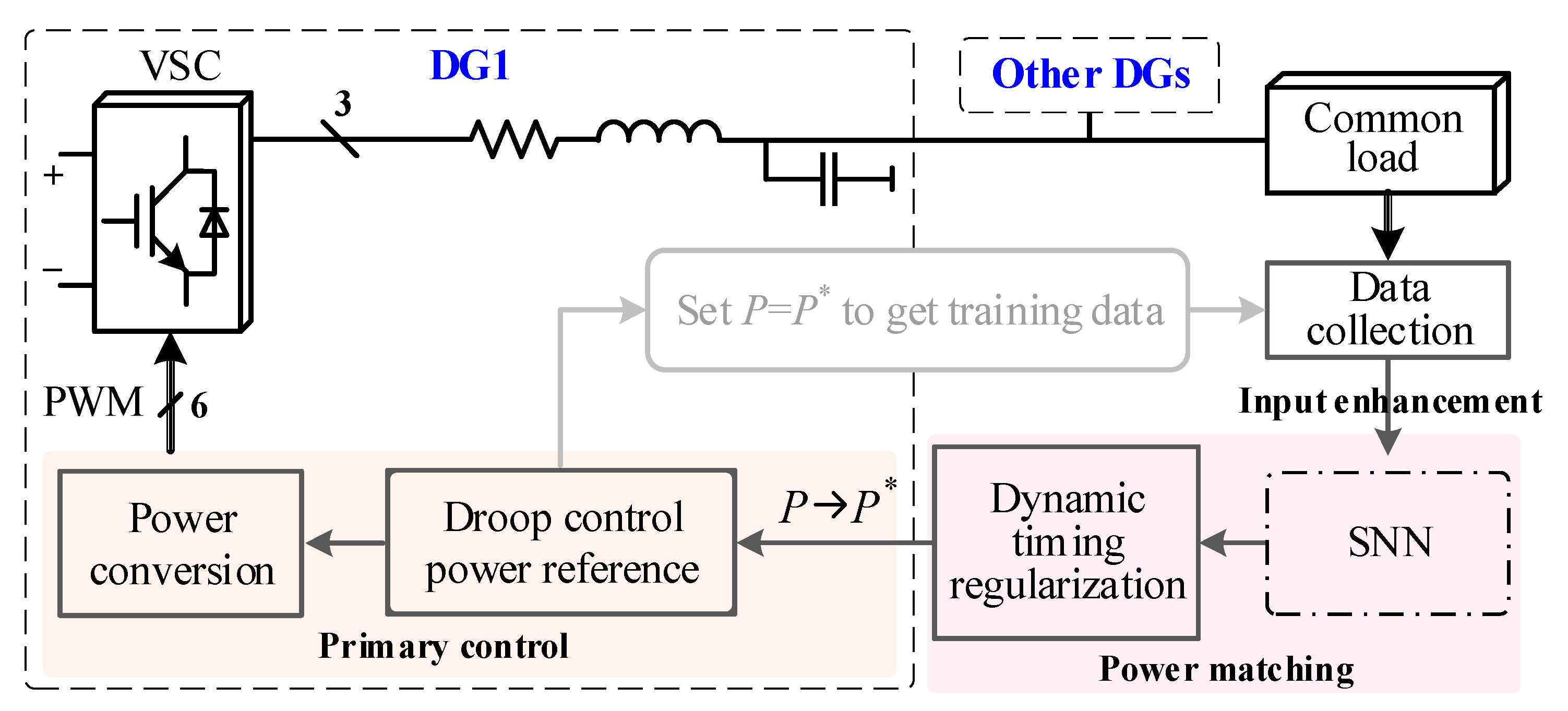
3.4. Overall Control Diagram

Figure 6 shows the overall control diagram of our proposed methods. The SNN collects variation data from the common load and processes it through input enhancement specific to the SNN. After training and prediction, it combines with dynamic timing regularization to match power commands with load consumption. This output feeds into the power reference setting of the droop control at the primary level. As a result, the system compensates for frequency deviation in the microgrid’s primary level, maintaining stability near the rated frequency. As for where the network training data comes from, as mentioned earlier, it is necessary to first obtain the droop control power reference value, set it as the power value required by each DG itself, and use this value to obtain training data by making the frequency reach its rated value.

Regarding the programming and time decision of the proposed approach, the hierarchical positioning can be explained from both dispatch-level and inverter-level perspectives. The SNN-based power fitting operates at the dispatch level, as it involves system-wide power allocation and matching between common load and individual DG controllers. The frequency deviation elimination is implemented at the inverter level, as it requires fast, localized control of individual inverters. The coordination between these two levels is achieved through a hierarchical control framework [29,30]. Specifically, the dispatch level sends power setpoints to the inverter level based on SNN predictions, and the inverter level fine-tunes these setpoints in real time to eliminate frequency deviations while respecting dispatch-level constraints.

The proposed algorithm, which incorporates droop control along with predictive and fitting methods, has been implemented in a microprocessor environment (such as DSP, FPGA, and other controllers, which are omitted here). This implementation enables efficient execution of control strategies vital for microgrid operations. The communication link plays a crucial role in the algorithm’s function, facilitating both the input of power reference values and the output of control compensation amounts. This ensures reliable information exchange for stable and efficient microgrid performance.

Regarding physical validation, while this study focuses primarily on simulation-based validation, the proposed SNN approach for microgrid frequency regulation could be verified through hardware-in-the-loop (HIL) or small-scale experimental setups in future work. A real-time digital simulator (e.g., OPAL-RT) could integrate either the trained neural network model or the microgrid model to test performance. Power conversion control algorithms could be implemented on programmable controllers such as DSP or FPGA development boards, creating a simple HIL architecture to test the effectiveness of the proposed control methods on the microgrid model in real time. Furthermore, an FPGA development board could act as a control unit, connected to a computer running the microgrid and control algorithms, to control the primary level in the simulation model and incorporate the SNN-trained power reference values. However, this physical validation will not be pursued in this paper.

4. Simulation Studies and Performance Assessment

To verify the effectiveness of the proposed SNN in terms of fitting performance, input data enhancement, and dynamic timing regularization, as well as to validate the scheme’s effect on frequency regulation, comprehensive simulation studies will be conducted below. The specifications and key parameters of the microgrid utilized here are presented in

Table 2. Specifications and key parameters for the microgrid system.

Description	Value
Microgrid
Rated frequency	50 Hz
Controller sampling time	4 × 10−5 s
DG1-DG3
Droop slope	m = 1 × 10−5
Local load	20 kW
Filter	0.02 Ω; 3.6 mH; 200 μF
DC source voltage	1 kV
Transmission Line
DG1	0.05 Ω; 1.2 mH
DG2	0.10 Ω; 2.4 mH
DG3	0.15 Ω; 3.6 mH
SNN
Hidden layer neurons	10
Input layer to hidden layer	tansig function
Hidden layer to output layer	purelin function
Input enhancement
Scaling value	α = 200

. The performance of the aforementioned methods will be demonstrated and compared sequentially. The studies construct a microgrid for testing three DGs using the system structure shown in Figure 1. The power of common load on the common AC bus changes dynamically with time; these variations follow those shown in Figure 2.

4.1. SNN

SNN training requires one-to-one correspondence between input and output data. As shown in Figure 2, this paper conducts SNN training for each of the three DGs separately, using their corresponding input and output data. The overall effect after network fitting is shown in Figure 7. The results indicate that the controller input power of all three DGs can effectively follow the ideal power variation curve, reflecting the overall change trend.

4.2. Input Enhancement

However, upon careful observation of Figure 7, there is still some latency in the data, and deviations exist between peak values. This misalignment is not ideal for frequency regulation. Before further data processing, the network training employs an input data enhancement method. This method not only improves the progress of network training but also reduces the number of required training epochs. Meanwhile, it achieves the same stability as previous SNN training.

Table 3. Training performance comparison.

Training Times	SNN			SNN with Input Enhancement
	Training Epochs	Gradient Values	RMSE	Training Epochs	Gradient Values	RMSE
1	287	6.60 × 10−8	3244.4896	267	2.06 × 10−8	3244.4976
2	291	2.02 × 10−8	3244.4948	224	6.87 × 10−8	3244.6135
3	229	9.26 × 10−8	3244.5632	230	7.56 × 10−8	3244.5714
4	241	8.16 × 10−8	3244.4918	209	8.70 × 10−8	3244.6388
5	209	8.26 × 10−8	3244.5627	226	2.84 × 10−8	3244.5948
Average	251.4	6.86 × 10−8	3244.5204	231.2	5.61 × 10−8	3244.5832

presents the comparison results between the two methods, showing average performance values from five testing rounds. In addition to the performance indicators shown in Table 3, both the SNN and SNN with input enhancement scenarios yield R values of 0.99062 and R² values of 0.98133 across these five runs. The results indicate that using the input data enhancement method can reduce the number of training epochs, thereby accelerating the training speed, which provides a faster solution for future real-time online operation.

The performance formulae involved here are as follows:

$$R={\displaystyle {\sum }_{i=1}^n(x_i-\overline{x})(y_i-\overline{y})}/\left(\sqrt{{\displaystyle {\sum }_{i=1}^n{(x_i-\overline{x})}^2}}\sqrt{{\displaystyle {\sum }_{i=1}^n{(y_i-\overline{y})}^2}}\right)$$

(18)

$$R^2=1-{\displaystyle {\sum }_{i=1}^n{(z_i-{\widehat{z}}_i)}^2}/{\displaystyle {\sum }_{i=1}^n{(z_i-\overline{z})}^2}$$

(19)

$$RMSE=\sqrt{{\displaystyle \frac{1}{n}}{\displaystyle {\sum }_{i=1}^n{(z_i-{\widehat{z}}_i)}^2}}$$

(20)

where x_i and y_i represent the true values and predicted values, respectively, $\overline{x}$ and $\overline{y}$ represent the mean of true values and predicted values, respectively, z_i is the actual observed value, ${\widehat{z}}_i$ is the predicted value, $\overline{z}$ is the mean of all actual observed values, and n is the sample size.

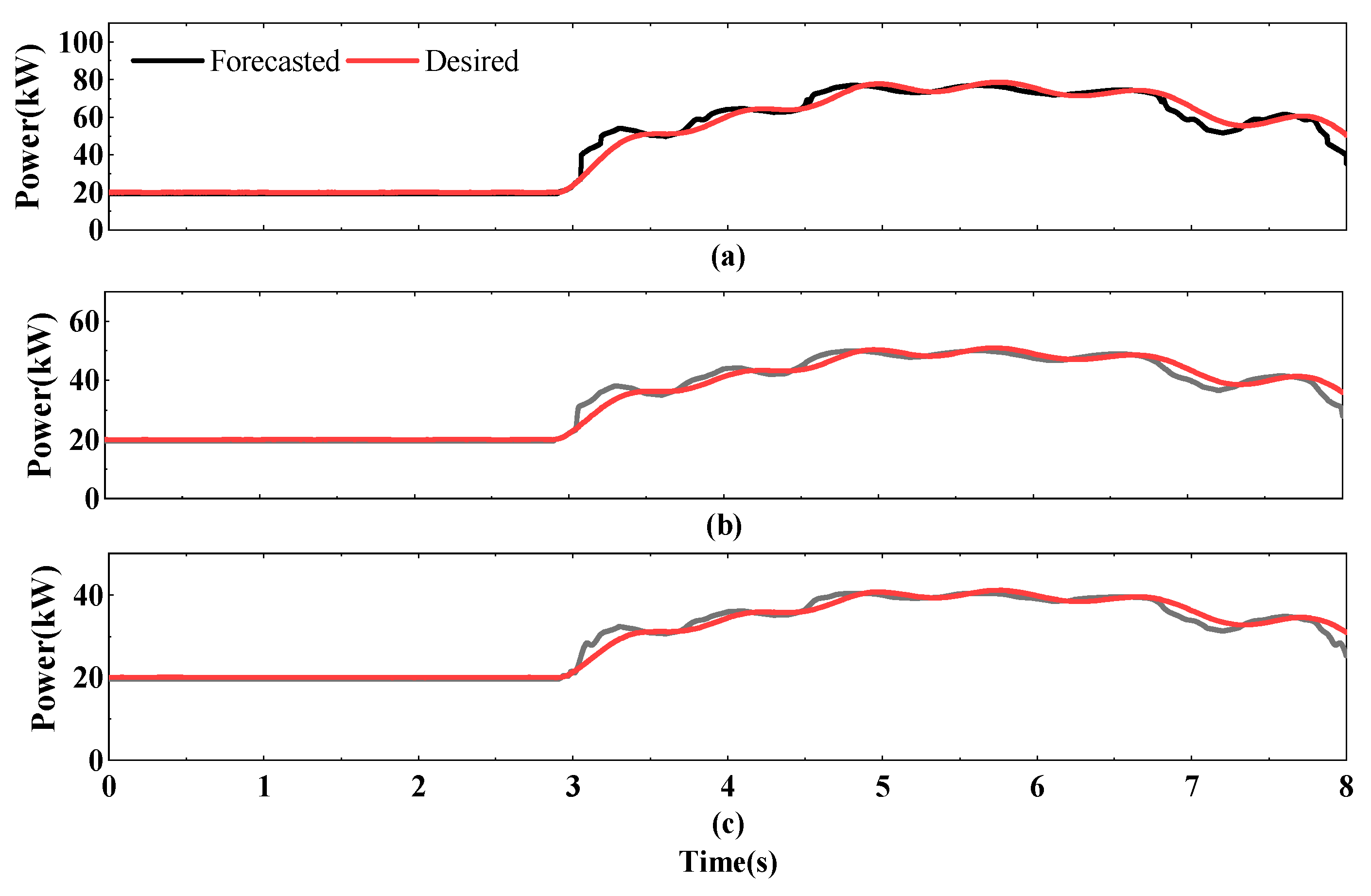
4.3. Control Effects Under SNN Fitting

As shown in Figure 8, when the primary level only uses droop power allocation (i.e., when the power reference value in Formula (1) is 0), the system frequency varies with changes in the common load. Under the droop control method, the frequency falls below the rated value of 50 Hz and decreases further as the common load power increases. When the common load power changes, the frequency changes accordingly. This frequency deviation from the rated value is undesirable, as it prevents equipment from operating at the rated frequency, thereby reducing system efficiency.

The system frequency curve when using SNN curve fitting is shown in Figure 9. Specifically, the SNN forecasted power values are used as power reference values in formula (1). Compared to Figure 8, it can be clearly seen that the system frequency has returned to near its rate value. Through SNN curve fitting, the effects of common load changes have been effectively counteracted, maintaining system frequency stability. The amplitude of frequency fluctuations and power distribution unevenness are related to line impedance, with these impedance values shown in Table 2 corresponding to each DG connection.

Analysis of the frequency operation curve shows that system frequency exhibits fluctuation characteristics when the common load changes, particularly with significant frequency fluctuations occurring after 3 s. These fluctuations mainly stem from two aspects: the deviation between SNN forecasted and actual values, and the deviation between peak values. Therefore, subsequent dynamic timing regularization is needed.

4.4. Dynamic Timing Regularization

As mentioned earlier, the curves obtained from SNN prediction still need dynamic adjustment between peak values to improve the accuracy of frequency regulation. Figure 10 shows the dynamic timing regularization effect of DG1 and its comparison with other cases. As can be seen from the figure, after dynamic regularization, compared to using SNN alone, the red line has become very close to the black time series line, even almost completely overlapping in some positions. Although, as shown in the magnified inset, there is still not absolute overlap, it has moved closer to the desired situation.

The implementation results when applying the time-regularized curves to frequency regulation are shown in Figure 11. Compared to Figure 9, the frequency fluctuations are significantly reduced, indicating that this method can more effectively resist the impact of dramatic changes in common load.

Taking DG1’s case for comparative analysis, as shown in Figure 12, the results further clearly demonstrate that better frequency regulation effects were achieved after applying SNN and dynamic timing regularization.

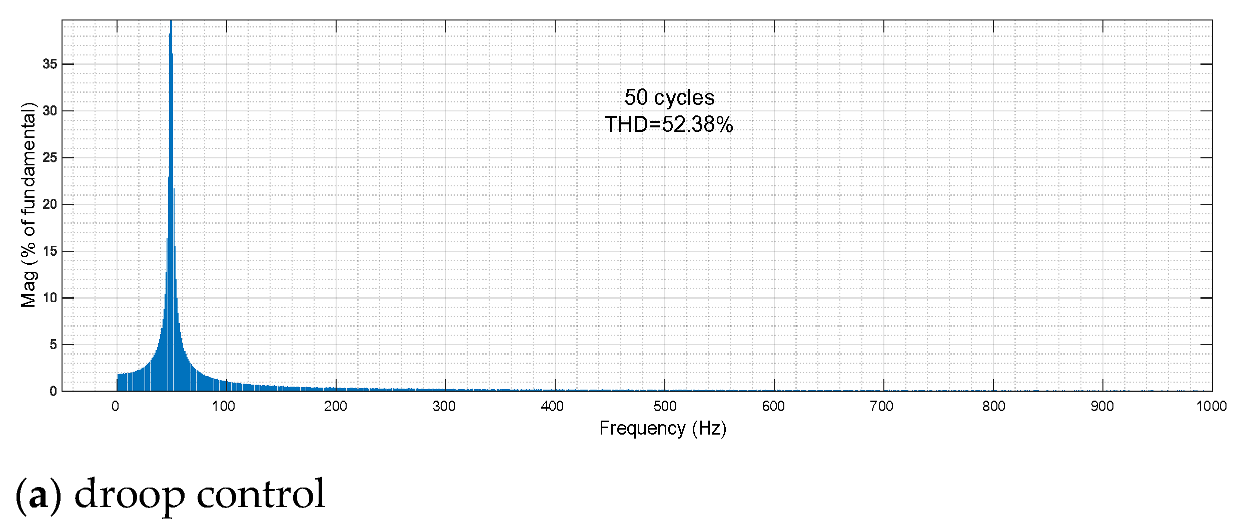
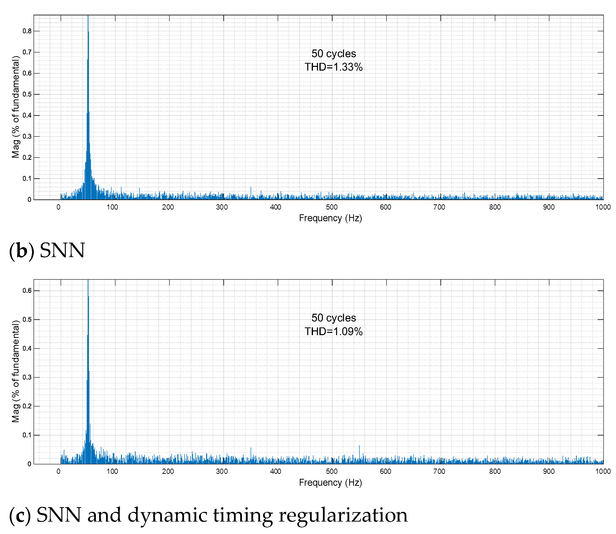
4.5. Voltage Waveform

In addition to the system frequency and power distribution curves, a comprehensive analysis of the voltage operation on the DG’s output ports was conducted. The results of the harmonic component analysis are shown in Figure 13. The study focuses on the voltage waveform of phase a of DG1, conducting a one-second test (50 cycles in total) starting from 5 s. This test duration helps avoid inaccurate voltage waveform assessment caused by random factors (general 2 cycles). The results reveal that power values derived from SNN fitting show a significant reduction in voltage waveform harmonic content, while dynamic timing regularization further improves and stabilizes voltage supply quality.

Figure 14 shows the real-time voltage waveforms and zoomed-in views under three scenarios during the one-second period from 5 s to 6 s. The results demonstrate that the proposed method achieves high-quality and stable voltage supply, which differs from using droop control alone. While using droop control, changes in common load power significantly affect the voltage phase waveform and frequency.

4.6. Comparison with Traditional Mathematical Matching Methods

A comparative analysis was conducted between the proposed methods and conventional mathematical matching approaches, with three distinct methods evaluated, as illustrated in Figure 15. Three methods are used for this comparison. The first method (Pload and proportional matching) achieves frequency regulation through proportional allocation based on fixed public load. This method adjusts the 1/3 distribution ratio of public load plus local load (20 kW), and uses the proportion coefficient of ideal total power output to match other DGs (DG1: 1, DG2: 0.7605, DG3: 0.6752), as shown by the blue line in the figure. The second method (constant ratio of common load) makes adjustments by setting coefficients (1.7 times) proportional to the public load. Results show that the frequency value is only affected when the public load has power output, as indicated by the black line in the figure. The third method (common load sharing) directly distributes the public load equally among each DG (1/3 each), without using compensation coefficients like the first method, as shown by the green line.

5. Conclusions

To address frequency regulation in microgrid systems, this paper proposes a mechanism of secondary frequency restoration through adjusting power reference values in primary-level droop control. The implementation uses SNNs to perform curve fitting between the common load power (set as inputs) and each DG system’s power (set as outputs) under ideal conditions. Through the use of input enhancement, the model trains faster and performs more consistently. Subsequently, dynamic timing regularization is employed to achieve precise peak-to-peak correspondence between curves. This method continuously enhances frequency regulation capability, enabling the microgrid to effectively resist power fluctuations from common loads. The effectiveness of these methods has been validated through detailed simulations and comparative analysis.

While this work explores how SNNs can enhance primary control and eliminate frequency deviation, modern DG systems face broader challenges that need further study, including transient instability during black-start events and misoperation under asymmetric grid conditions. Future research will investigate how artificial intelligence methods can detect faults and tune droop settings to prevent these failures, especially in industrial-scale DG systems. Furthermore, the proposed approaches could scale to larger microgrids with heterogeneous resources and loads. The SNNs only need to establish variable input-output relationships between common load and each DG, while frequency elimination does not hinder DG expansion due to the discrete nature of droop control. However, it is important to note that the proposed methods have limitations, particularly when dealing with large, real-time fluctuations in common load, which can challenge SNN training and may require high-performance training systems.

References

1. Theocharides, S.; Theristis, M.; Makrides, G.; Kynigos, M.; Spanias, C.; Georghiou, G.E. Comparative Analysis of Machine Learning Models for Day-Ahead Photovoltaic Power Production Forecasting. Energies 2021, 14, 1081. [Google Scholar] [CrossRef]
2. Hu, J.; Shan, Y.; Guerrero, J.M.; Ioinovici, A.; Chan, K.W.; Rodriguez, J. Model Predictive Control of Microgrids—An Overview. Renew. Sustain. Energy Rev. 2021, 136, 110422. [Google Scholar] [CrossRef]
3. Wang, G.; Wang, X.; Wang, F.; Han, Z. Research on Hierarchical Control Strategy of AC/DC Hybrid Microgrid Based on Power Coordination Control. Appl. Sci. 2020, 10, 7603. [Google Scholar] [CrossRef]
4. Lee, J.O.; Kim, Y.S. Frequency and State-of-Charge Restoration Method in a Secondary Control of an Islanded Microgrid without Communication. Appl. Sci. 2020, 10, 1558. [Google Scholar] [CrossRef]
5. Ning, B.; Han, Q.L.; Zuo, Z.; Ding, L. Accelerated Secondary Frequency Regulation and Active Power Sharing for Islanded Microgrids with External Disturbances: A Fully Distributed Approach. Automatica 2025, 174, 112146. [Google Scholar] [CrossRef]
6. Dangeti, L.s.n.; R., M. Distributed Model Predictive Control Strategy for Microgrid Frequency Regulation. Energy Rep. 2025, 13, 1158–1170. [Google Scholar] [CrossRef]
7. Chen, Y.; Qi, D.; Hui, H.; Yang, S.; Gu, Y.; Yan, Y.; Zheng, Y.; Zhang, J. Self-Triggered Coordination of Distributed Renewable Generators for Frequency Restoration in Islanded Microgrids: A Low Communication and Computation Strategy. Adv. Appl. Energy 2023, 10, 100128. [Google Scholar] [CrossRef]
8. Agundis Tinajero, G.D.; Guerrero, J.M. Power Flow Modeling for Battery Energy Storage Systems with Hierarchical Control for Islanded Microgrids. Electronics 2024, 13, 4927. [Google Scholar] [CrossRef]
9. Wang, Y.; Shi, J.; Ma, N.; Liu, G.; Xin, L.; Liu, Z.; Liu, D.; Xu, Z.; Chen, C. An Improved Secondary Control Strategy for Dynamic Boundary Microgrids toward Resilient Distribution Systems. Energies 2024, 17, 1731. [Google Scholar] [CrossRef]
10. Chen, W.; Wang, Z.; Liu, Q.; Yue, D.; Liu, G.P. A New Privacy-Preserving Average Consensus Algorithm with Two-Phase Structure: Applications to Load Sharing of Microgrids. Automatica 2024, 167, 111715. [Google Scholar] [CrossRef]
11. Shan, Y.; Hu, J.; Shen, B. Distributed Secondary Frequency Control for AC Microgrids Using Load Power Forecasting Based on Artificial Neural Network. IEEE Trans. Ind. Inf. 2024, 20, 1651–1662. [Google Scholar] [CrossRef]
12. Belgana, S.; Fortin-Blanchette, H. A Novel Neural Network-Based Droop Control Strategy for Single-Phase Power Converters. Energies 2024, 17, 5825. [Google Scholar] [CrossRef]
13. Elsaraiti, M.; Merabet, A. A Comparative Analysis of the Arima and Lstm Predictive Models and Their Effectiveness for Predicting Wind Speed. Energies 2021, 14, 6782. [Google Scholar] [CrossRef]
14. Mahim, T.M.; Rahim, A.H.M.A.; Rahman, M.M. Adaptive Fuzzy Attention Inference to Control a Microgrid Under Extreme Fault on Grid Bus. IEEE Trans. Fuzzy Syst. 2025. [Google Scholar] [CrossRef]
15. Manno, A.; Martelli, E.; Amaldi, E. A Shallow Neural Network Approach for the Short-Term Forecast of Hourly Energy Consumption. Energies 2022, 15, 958. [Google Scholar] [CrossRef]
16. Trivedi, R.; Khadem, S. Implementation of Artificial Intelligence Techniques in Microgrid Control Environment: Current Progress and Future Scopes. Energy AI 2022, 8, 100147. [Google Scholar] [CrossRef]
17. Huang, Y.; Li, G.; Chen, C.; Bian, Y.; Qian, T.; Bie, Z. Resilient Distribution Networks by Microgrid Formation Using Deep Reinforcement Learning. IEEE Trans. Smart Grid 2022, 13, 4918–4930. [Google Scholar] [CrossRef]
18. Fang, X.; Khazaei, J. A Two-Stage Deep Learning Approach for Solving Microgrid Economic Dispatch. IEEE Syst. J. 2023, 17, 6237–6247. [Google Scholar] [CrossRef]
19. Shao, W.; Li, X.; Xing, Y.; Chen, J. A Mixture of Shallow Neural Networks for Virtual Sensing: Could Perform Better than Deep Neural Networks. Expert Syst. Appl. 2024, 256, 124870. [Google Scholar] [CrossRef]
20. Gong, J.; Qu, Z.; Zhu, Z.; Xu, H.; Yang, Q. Ensemble Models of TCN-LSTM-LightGBM Based on Ensemble Learning Methods for Short-Term Electrical Load Forecasting. Energy 2025, 318, 134757. [Google Scholar] [CrossRef]
21. Suto, J.; Oniga, S. Efficiency Investigation from Shallow to Deep Neural Network Techniques in Human Activity Recognition. Cogn. Syst. Res. 2019, 54, 37–49. [Google Scholar] [CrossRef]
22. Bejani, M.M.; Ghatee, M. A Systematic Review on Overfitting Control in Shallow and Deep Neural Networks. Artif. Intell. Rev. 2021, 54, 6391–6438. [Google Scholar] [CrossRef]
23. Onifade, M.; Lawal, A.I.; Bada, S.O.; Khandelwal, M. Predictive Modelling for Coal Abrasive Index: Unveiling Influential Factors through Shallow and Deep Neural Networks. Fuel 2024, 374, 132319. [Google Scholar] [CrossRef]
24. Mishra, B.; Pattnaik, M. A Modified Droop-Based Decentralized Control Strategy for Accurate Power Sharing in a PV-Based Islanded AC Microgrid. ISA Trans. 2024, 153, 467–481. [Google Scholar] [CrossRef]
25. Wu, L.; Yang, H.; Wei, J.; Jiang, W. Research on Distributed Coordination Control Method for Microgrid System Based on Finite-Time Event-Triggered Consensus Algorithm. Chin. J. Electr. Eng. 2024, 10, 103–115. [Google Scholar] [CrossRef]
26. Yogithanjali Saimadhuri, K.N.; Janaki, M. Advanced Control Strategies for Microgrids: A Review of Droop Control and Virtual Impedance Techniques. Results Eng. 2025, 25, 103799. [Google Scholar] [CrossRef]
27. Zhang, Z.; Han, T.; Huang, C.; Shuai, C. Hardware and Software Design and Implementation of Surface-EMG-Based Gesture Recognition and Control System. Electronics 2024, 13, 454. [Google Scholar] [CrossRef]
28. Huang, J.; Qin, H.; Shen, K.; Yang, Y.; Jia, B. Study on Hierarchical Model of Hydroelectric Unit Commitment Based on Similarity Schedule and Quadratic Optimization Approach. Energy 2024, 305, 132229. [Google Scholar] [CrossRef]
29. Shan, Y.; Ma, L.; Yu, X. Hierarchical Control and Economic Optimization of Microgrids Considering the Randomness of Power Generation and Load Demand. Energies 2023, 16, 5503. [Google Scholar] [CrossRef]
30. Wu, X.; Shan, Y.; Fan, K. A Modified Particle Swarm Algorithm for the Multi-Objective Optimization of Wind/Photovoltaic/Diesel/Storage Microgrids. Sustainability 2024, 16, 1065. [Google Scholar] [CrossRef]
Figure 1. AC microgrid topology.
Asi 08 00067 g001
Figure 2. Curves of input-output data that need to be fitted.
Asi 08 00067 g002
Figure 3. SNN topology.
Asi 08 00067 g003
Figure 4. Flowchart for SNN fitting.
Asi 08 00067 g004
Figure 5. Complete flowchart for data processing.
Asi 08 00067 g005
Figure 6. Overall control diagram.
Asi 08 00067 g006
Figure 7. Comparison between SNN forecasted and desired curves. (a) DG1, (b) DG2, (c) DG3.
Asi 08 00067 g007
Figure 8. System performance under droop control. (a) frequency, (b) power sharing.
Asi 08 00067 g008
Figure 9. System performance using SNN curve fitting. (a) frequency, (b) power sharing.
Asi 08 00067 g009
Figure 10. Comparison of DG1’s dynamic timing regularization effects with other scenarios.
Asi 08 00067 g010
Figure 11. System performance using SNN and dynamic timing regularization. (a) frequency, (b) power sharing.
Asi 08 00067 g011
Figure 12. Comparison of DG1’s performance effects. (a) frequency, (b) power sharing.
Asi 08 00067 g012
Figure 13. Quality analysis of DG1 a-phase voltage waveform starting at 5 s for 50 cycles lasting 1 s.
Asi 08 00067 g013aAsi 08 00067 g013b
Figure 14. Voltage waveform from 5 s to 6 s.
Asi 08 00067 g014
Figure 15. Comparison with other mathematical matching methods.
Asi 08 00067 g015