1. Introduction
Nowadays, the fields of electrical energy production have become of vital importance in industrial factories characterized by their energy-intensive aspect, in particular those whose manufacturing processes allow the release of thermal energy. This importance is seen mainly in the possibility of achieving the self-sufficiency in electrical energy, so as to cover partially or totally the internal consumption of the plant.
The industrial method most commonly used in this sense is to recover the heat released by these processes into tubular exchangers by evaporating the feed water in the thermal boilers. Then, the steam produced is used under pressure to drive a turbine coupled to an electricity generator.
Nevertheless, the prediction of produced electricity has now become a key factor in reducing the energy bills of factories, which is why it is necessary to construct Artificial Intelligence (AI) models to control and master upstream the factors that create undesirable reductions in or disruptions to electrical power.
The structure of this work is as follows:
Section 2 presents state-of-the-art techniques previously used by scientific researchers to predict electrical power;
Section 3 discusses the three methods we employed for prediction, starting with a technical framework of our case study.
Section 4 presents the results of the developed models including a comparison of their performance.
Section 5 discusses and interprets the obtained results.
Section 6 provides the conclusion, which highlights the benefits of these contributions, as well as some perspectives.
2. Related Works Linked to the Prediction of Electrical Power
In this section, we present a summary of the most recent research works related to the subject. This summary is shown in
Table 1 with various case studies.
It should be noted that the research works on electrical power prediction cited above mainly focused on consumption rather than production.
Similarly, although they used various algorithms, they were more oriented toward renewable sources than fossil energies. We suggest that some of the works required more research efforts to optimize their uses, especially in the case of steam power plants.
In the present work, we aim to shed light on the prediction of power at the production level and the level of a steam power plant associated with an industrial exothermal process linked to the combustion of sulfur as a raw material.
3. Materials and Methods
This section focuses on the framing of the problem of our case study, the exploration of the data required to develop the solution, as well as the presentation of the techniques used for the prediction of electrical power production.
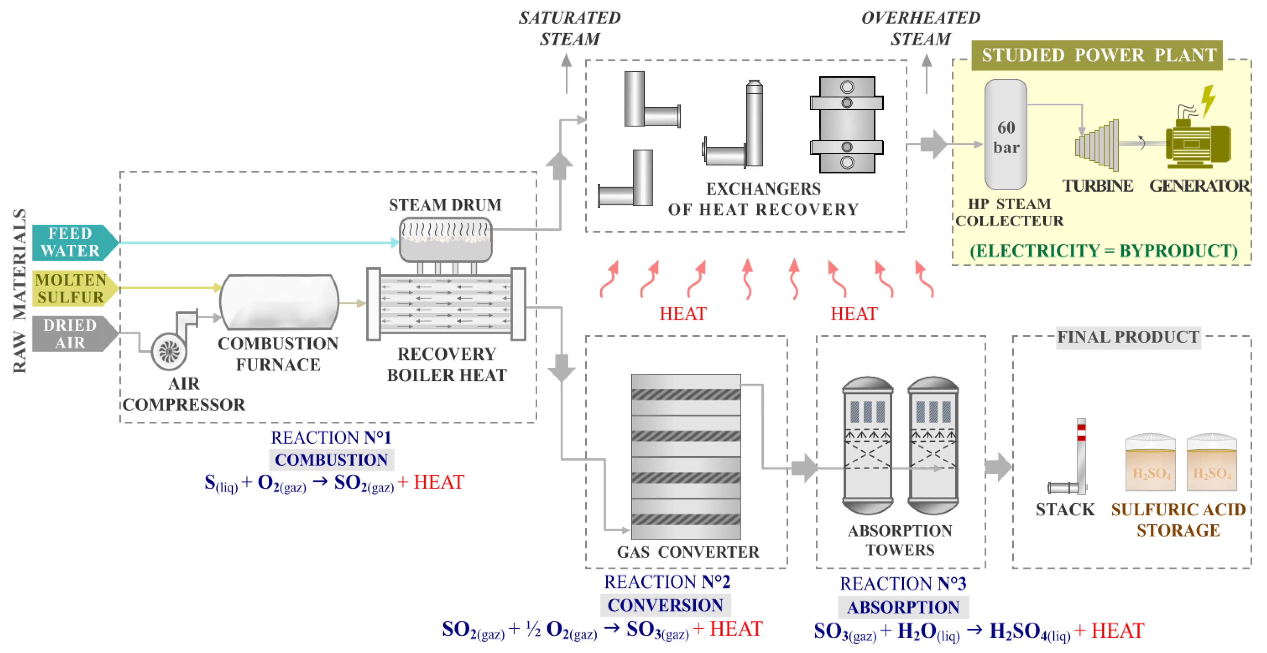
3.1. Industrial Process Description
The application considered is an industrial process in a thermal power plant for the production of electrical energy, which is associated with a sulfuric acid production line, as presented in (
Figure 1).
The plant is continuously supplied with high-pressure steam due to the exothermic nature of the sulfuric line process. Therefore, electricity is produced through the mechanical drive of a turbine coupled with an alternator.
Then, the local electrical network ensures the internal self-supply of energy, which could also be connected to the distribution grid of the public operator to ensure an electrical exchange.
3.2. Dataset Presentation
Before preparing the dataset, it should be noted that the construction of the models was carried out on a platform using Python as a computing tool.
To achieve the objective of the study, we collected numerical data from a factory using the same aforementioned production process. The data covered a period of 6 months, with 1 value recorded every five 5 min as the sampling frequency, i.e., a total of 51,840 data points.
According to the analysis of the process history, there are five main parameters related to steam that impact the variation in the electrical power generation in megawatts (MW), which are presented in
Table 2.
The rated capacity of the alternator dedicated to this application is 58 MW, which also has a rated apparent power of 68 MVA.
3.3. Correlation Analysis
The accuracy of the models depends significantly on the correlation between the variables used. Thus, it is necessary to evaluate the correlation of different inputs with the outputs of power production. The calculation of these coefficients before constructing the models can give us a clear idea about the highly correlated parameters and weakly correlated parameters.
In mathematics and statistics, covariance is a measure of the relationship between two random variables, whereas correlation is a measure of the strength of the relationship between the variables. In other words, correlation is the scaled measure of covariance.
The mathematical formulas for covariance (1) and correlation (2) are as follows:
where
Xi is the values of the X variable.
Yi is the values of the Y variable.
is the mean value (average) of the X variable.
is the mean value (average) of the Y variable.
N is the number of data points.
σX is the standard deviation of the X variable.
σY is the standard deviation of the Y variable.
It was expected in this work that the dependency relationships between several variables can be represented by a correlation matrix in Python.
3.4. Considered Deep Learning Algorithms
3.4.1. Long Short-Term Memory (LSTM)
Before explaining LSTM, it is important to understand recurrent neural networks (RNN) given the close relationship between them. The structure of the RNN consists of an input layer, one or more hidden layers, and an output layer. RNNs have chain-like structures of repeating modules, which are used as memory for storing important information from previous processing steps [
15].
LSTM is an evolution of RNNs and was introduced to eliminate the drawbacks of RNNs related to vanishing / exploding gradients and rectify the problems of the short memory linked to RNNs by adding complementary interactions per cell.
3.4.2. Convolutional Neural Network (CNN)
There are two types of convolutional neural networks, biological neural networks and artificial neural networks. This work mainly discusses artificial neural networks.
A CNN-based artificial neural network is a modeling method that promotes data and is similar in form to the synaptic links of the human brain. It is composed of several neurons; the output of the previous neuron can serve as the input of the next neuron.
To sum up, the structural diagram of the CNN algorithm is composed of an “Input Layer” that is connected to an “Output Layer” through three steps: “the Convolution Layer n°1”, “the Convolution Layer n°2”, and a “Hidden Layer” [
16].
3.4.3. CNN-LSTM Hybrid Model
A CNN (convolutional neural network) model consists of three layers: an input layer, a hidden layer, and an output layer. The input of a three-dimensional array is usually fed into a convolutional layer, where the dimensions are represented by the height, weight, and number of channels [
17].
Both CNN and LSTM models have specific features. Thus, a hybrid CNN–LSTM DL model was considered in this study, which includes the advantages of both CNN and LSTM models.
3.5. Assessment Strategy for the Models
Since we are working on a regression problem linked to archived historical data, we evaluated the studied models using the following metrics: the RMSE (root mean square error) [
18] governed by Equation (3), the MSE (mean square error) [
19] described by Equation (4), and R-squared (explained variance score) expressed by Equation (5).
where
i is the actual value of y of the target variable (measured value of electrical power).
is the predicted value of y of the target variable (predicted value of electrical power).
is the mean value of y of the target variable (mean value of electrical power).
N is the number of samples related to the prediction.
4. Results
Before presenting the results, we note that for each model, the used dataset was divided into two sub-samples. The first was the learning sample (80% of the scope of the dataset) and the second was the validation sample (20% of the scope of the dataset).
Each model was built on the training sample and validated on the test sample with a performance score.
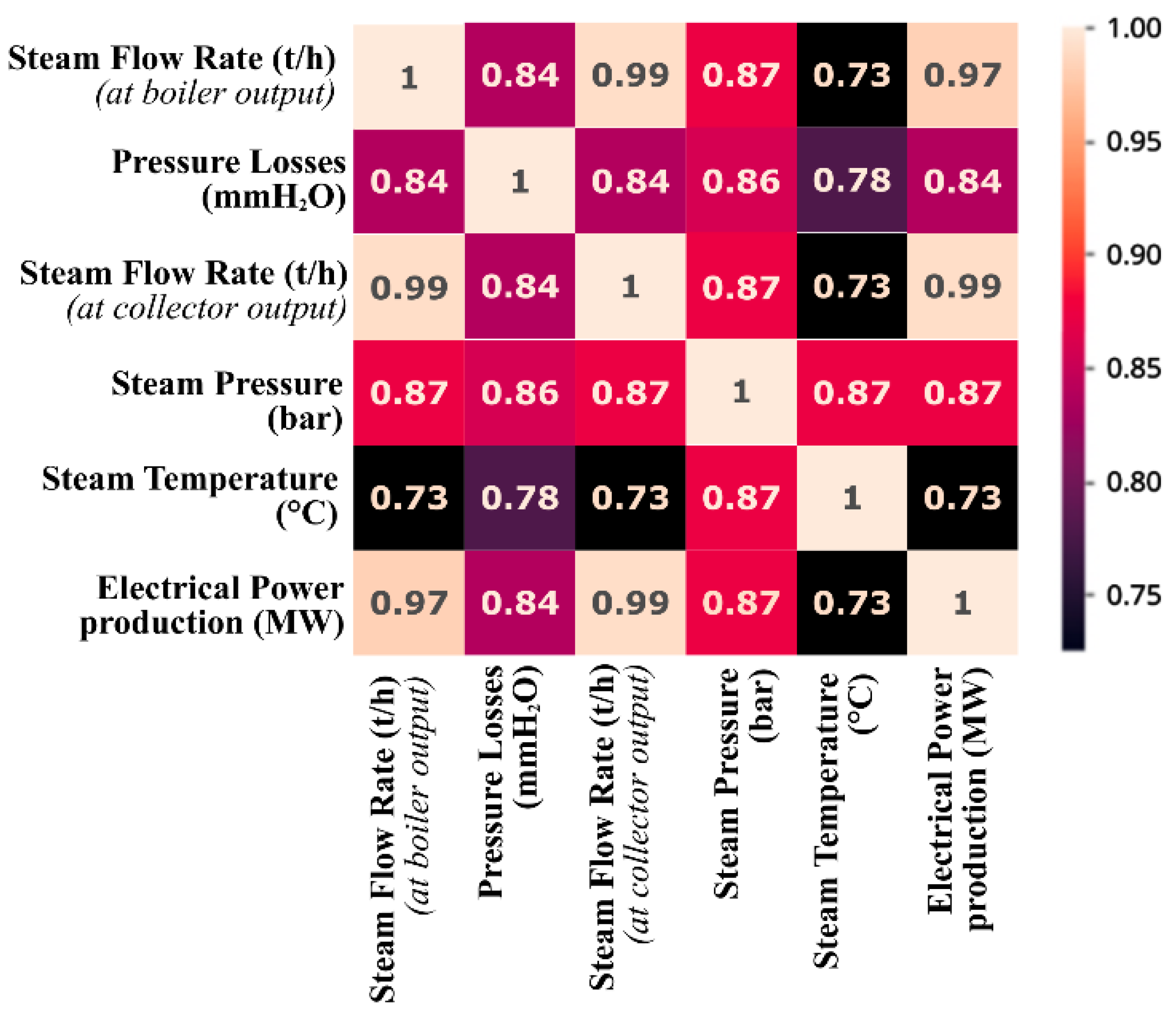
4.1. Correlation Check between Variables
By performing a dependency analysis between the studied parameters, we generated the corresponding correlation matrix in
Figure 2, which is based on the heat map concept.
4.2. Theoretical Interpretation of Correlation Results
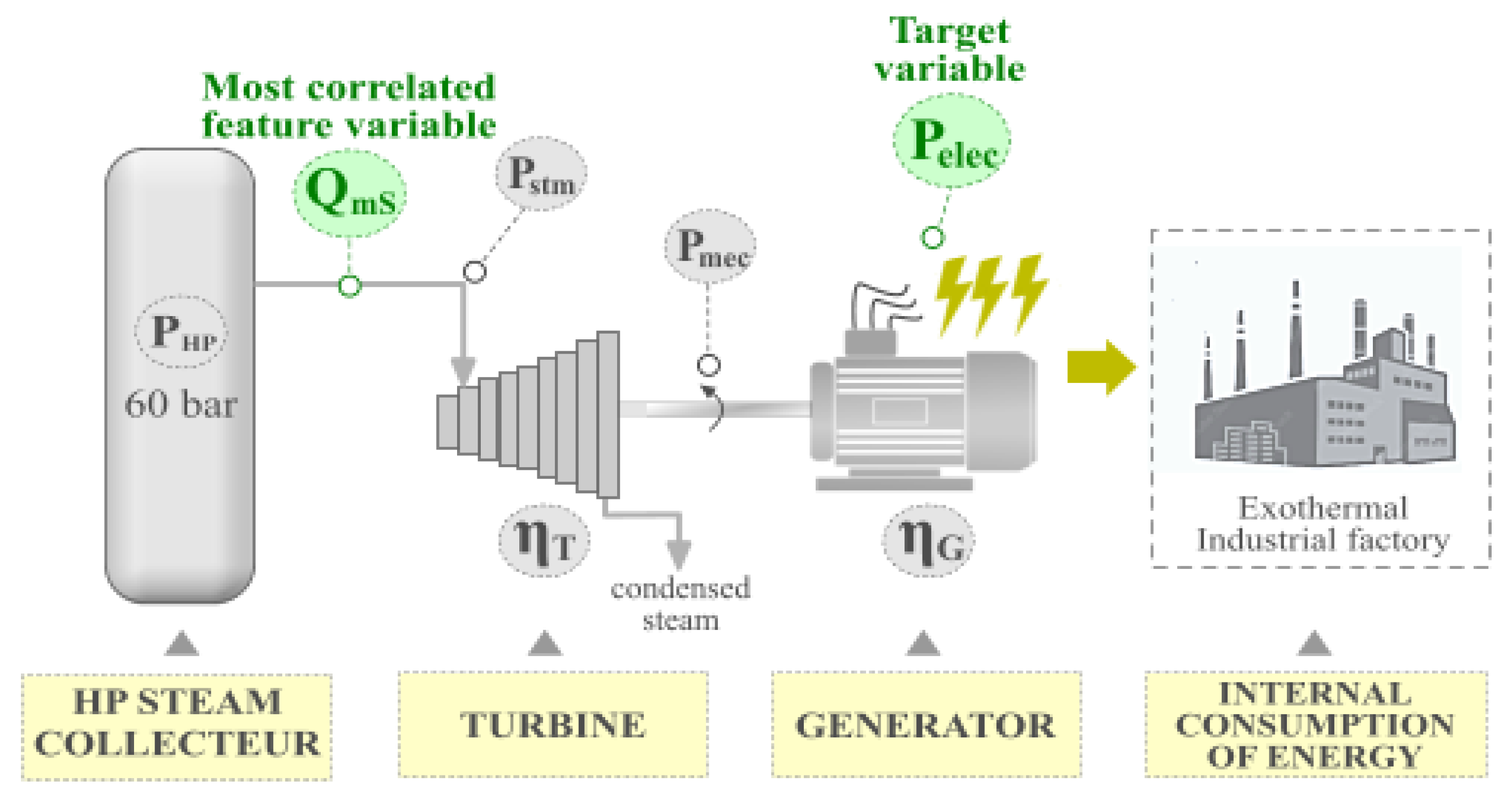
As seen in the above matrix, the parameter « Steam Mass flow rate QmS » had the highest dependency relationship with the target parameter (Pelec).
We demonstrated theoretically that this strong dependence was justified by a physical link between these two parameters, as seen in
Figure 3.
By applying the first law of thermodynamics [
20] to the HP steam turbine following the Rankine cycle model, the internal energy is expressed as follows:
where
is the variation in enthalpy (kJ).
variation in kinetic energy (kJ).
variation in potential energy (kJ).
calorific energy (kJ).
is the work carried out on the system (kJ).
By considering the following hypotheses of the Rankine cycle:
- -
the transformation is adiabatic
- -
the linear velocity is constant (
- -
the altitude is constant
Likewise, by multiplying the work by the mass flow rate of the steam
, we obtain the useful power of the steam
:
is the power of the steam (kW).
is the variation of enthalpy (kJ).
is the mass flow rate of steam at collector output (t/h).
is the mass of the steam (tons).
Otherwise, we calculate the global efficiency of the steam turbine [
21] coupled with the generator:
where
is the global efficiency of the turbine generator.
is the efficiency of the turbine.
is the efficiency of the generator.
is the global losses at the level of the turbine (kW).
is the global losses at the level of the generator (kW).
Considering the fact that losses tend to zero, we obtain
According to Equations (9) and (13), we deduce
where K is a positive coefficient that is equal to
From Equation (14), we observe that there is a direct proportional relationship between the target variable (Pelec) and its most correlated feature (Qms).
Thus, the correlation of 99% found automatically through Python is physically justified.
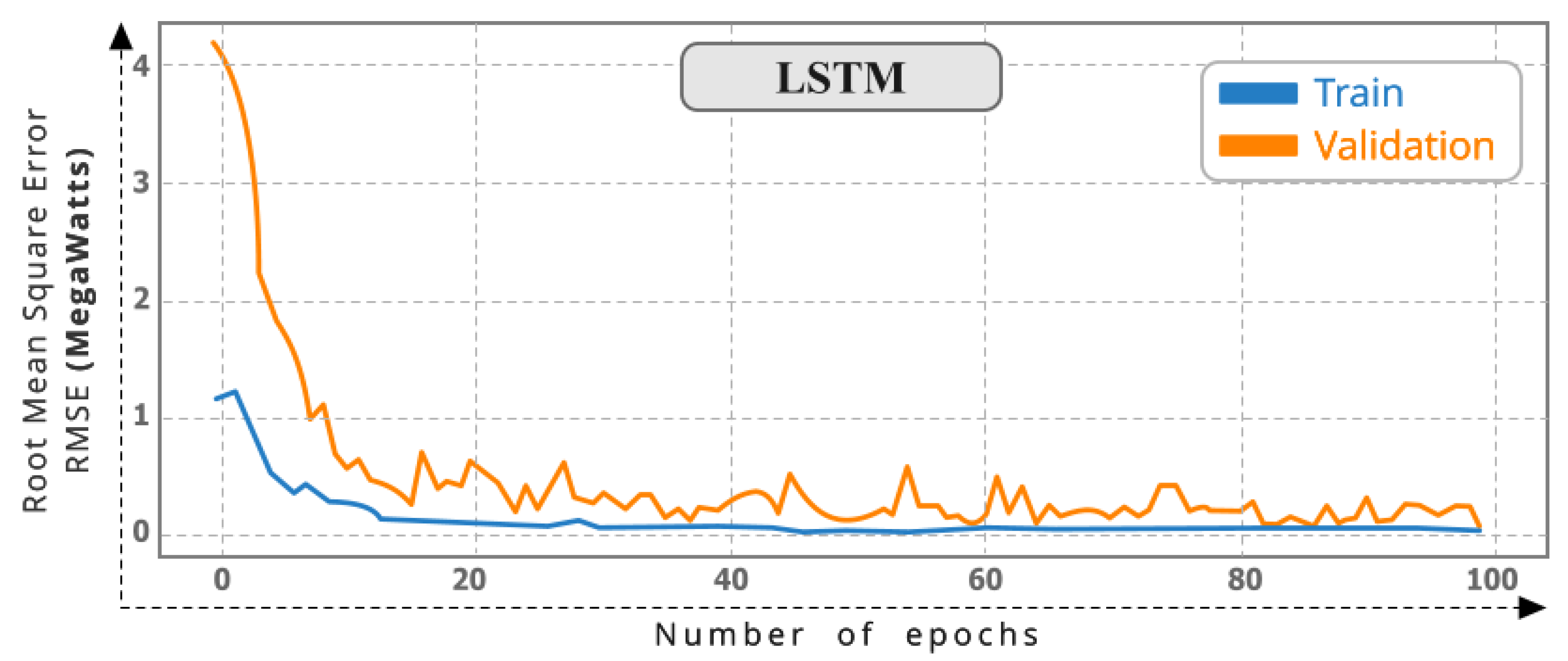
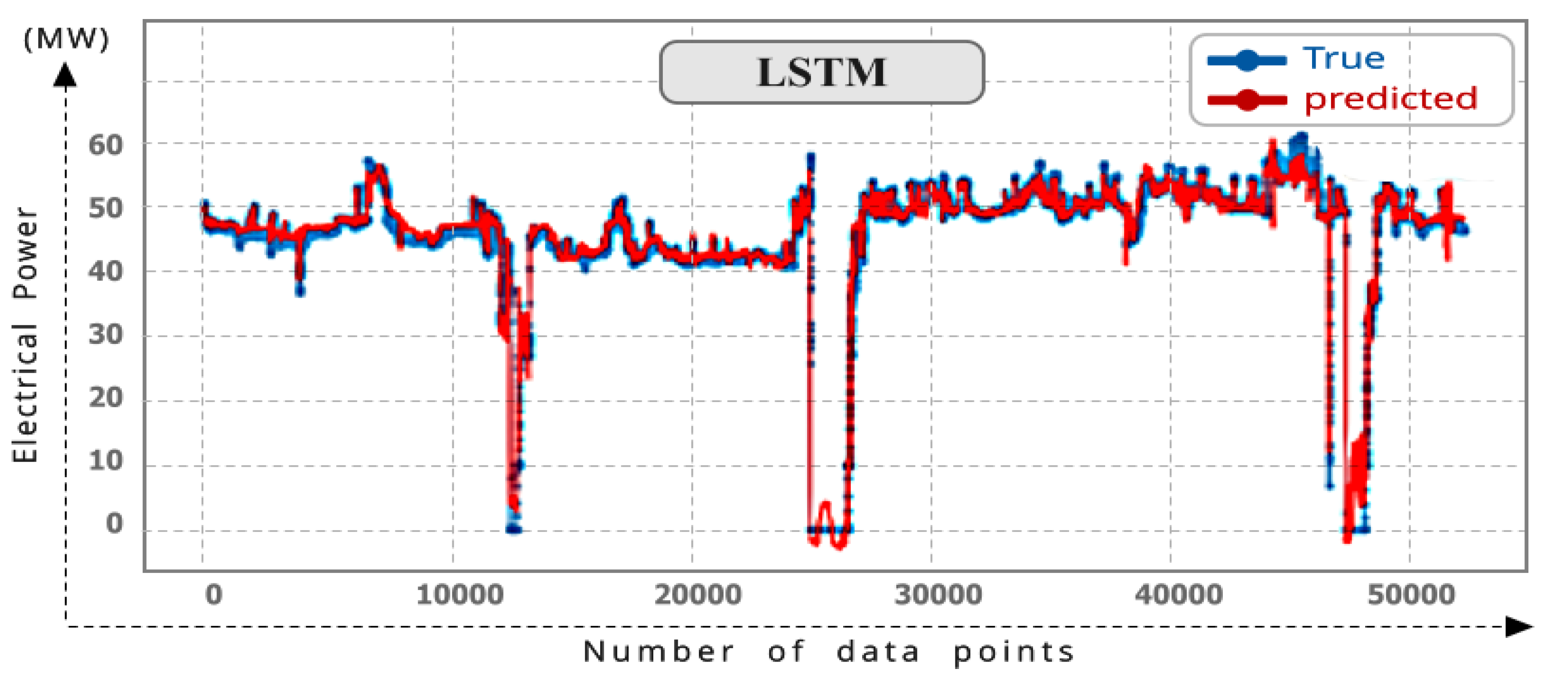
4.3. Results of Electrical Power Prediction Using LSTM Model
The result of this phase is described in the
Figure 4 below.
The result of this phase is described in the
Figure 5 below.
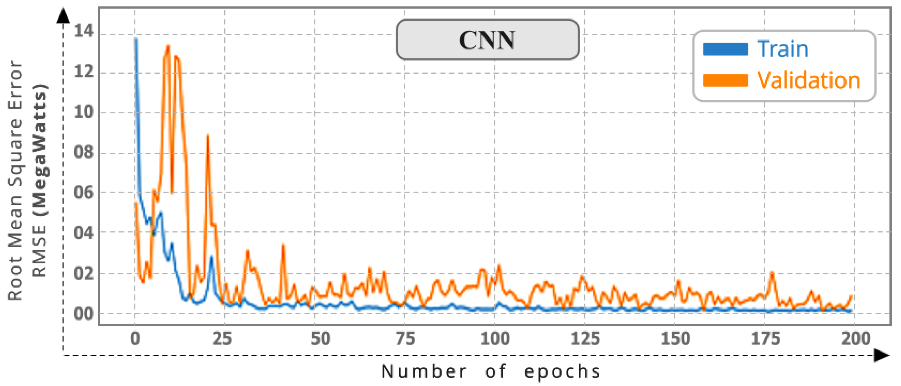
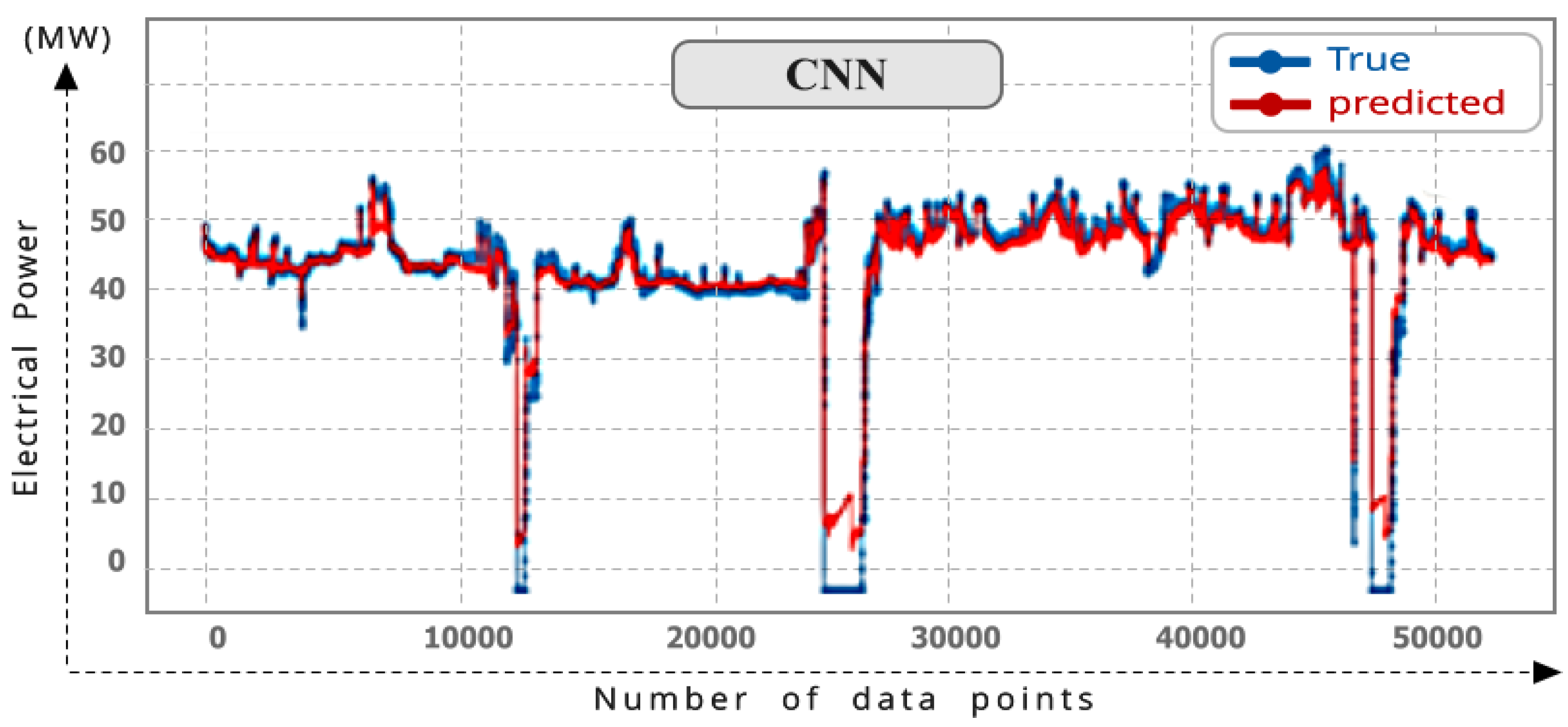
4.4. Results of Electrical Power Prediction Using CNN Model
The result of this phase is described in the
Figure 6 below.
The result of this phase is described in the
Figure 7 below.
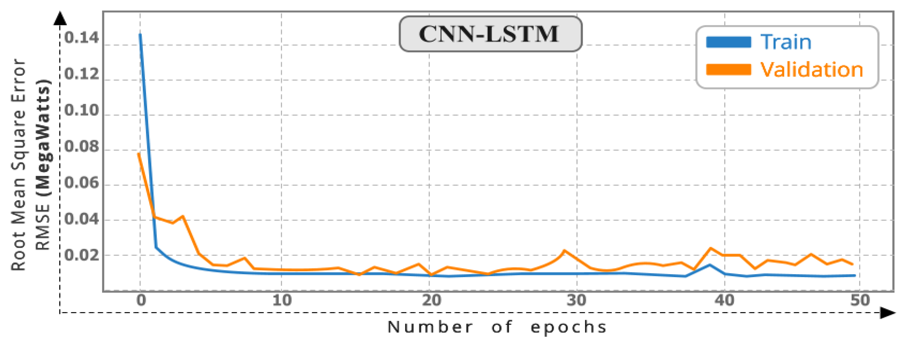
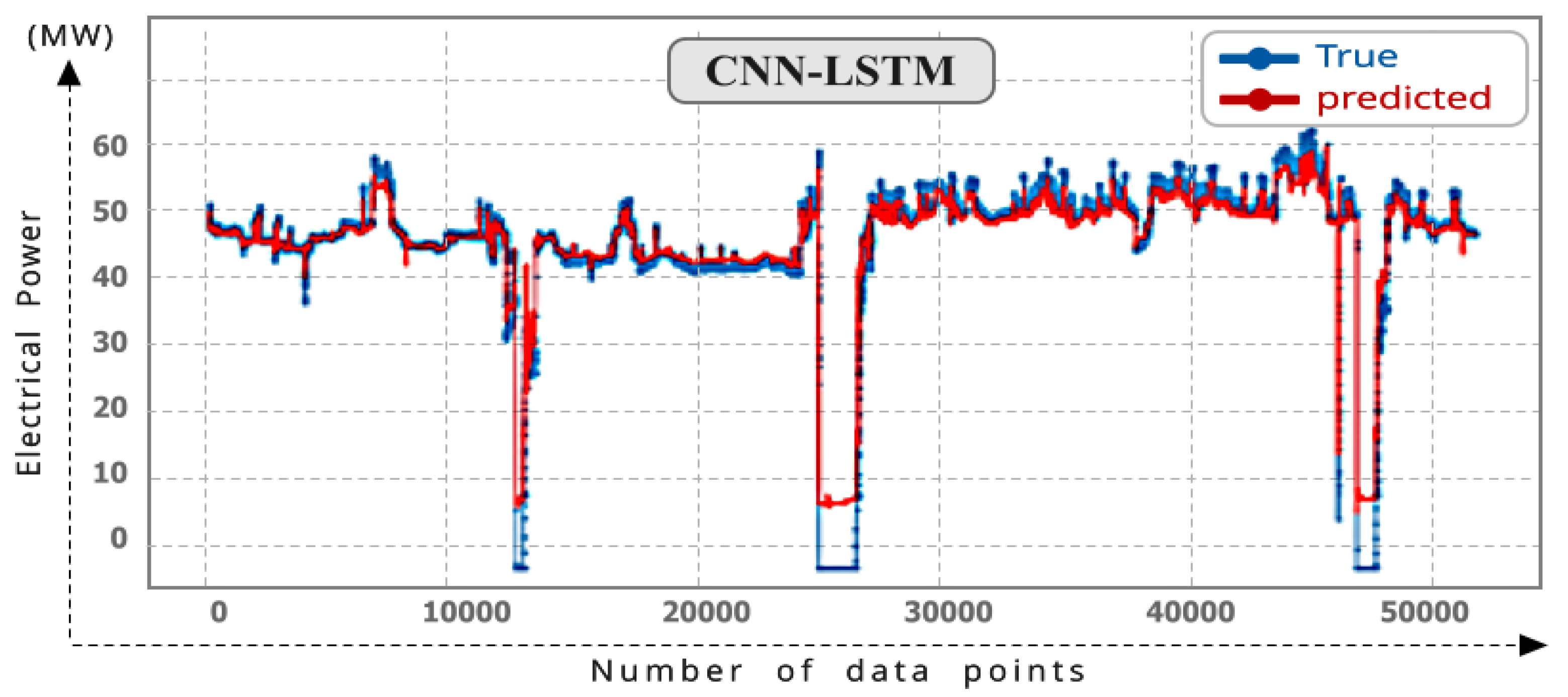
4.5. Results of Electrical Power Prediction Using CNN-LSTM Hybrid Model
The result of this phase is described in the
Figure 8 below.
The result of this phase is described in the
Figure 9 below.
4.6. Performance Metrics Comparison of the Constructed Models
The results obtained by the calculation of the evaluation metrics are presented in (
Table 3), which also shows a comparison of the performance achieved by each prediction model.
5. Discussion
5.1. Findings
As observed in the correlation analysis in
Figure 2, the variables “Steam Flow Rate at the collector output” and “Steam Flow Rate at the Boiler output” had the strongest dependencies on the target variable studied with correlations of 99% and 97%, respectively. They were followed by the parameters “Steam Pressure” and “Pressure Losses”, with respective dependencies of 87% and 84%. Finally, the variable “Steam Temperature” correlated with electrical power with a percentage of 73%.
We then deduced that all predefined parameters had a significant correlation with the target variable. It is therefore appropriate to retain all of them to train and test the studied models.
On the other hand, and in light of the performance results obtained in (
Table 3), the model based on the long short-term memory (LSTM) algorithm offered a better quality of prediction of the electrical power parameter. This performance was seen in the R-squared metric score, which was the highest (≈98.39%). However, the scores of the two metrics RMSE and MSE, which interpreted the errors, were, respectively, 0.241 MW and 0.058 MW.
Similarly, and by training the model based on the CNN-LSTM algorithm, we were able to maintain a high R-squared score (≈98.29%) and also minimize the error margins generated by LSTM to achieve an RMSE of 0.1199 MW and MSE equal to 0.0143 MW. This improvement confirmed that the CNN-LSTM hybrid mode is very suitable for power prediction.
As for the convolutional neural network (CNN) algorithm, its performance was less acceptable given that its score was also high (R2 = 94.66%), except that the margin of error was greater than that of the two previous models, with an RMSE of 0.4301 MW and an MSE of 0.1849 MW, which makes this model ranked third in our comparative study.
To allow a more complete analysis of the models, the loss curves were drawn during the training phase and are presented in
Figure 4 for the LSTM model,
Figure 6 for the CNN model, and
Figure 8 for the CNN-LSTM model. In this sense, the LSTM algorithm reached its maximum score (98%) after 100 epochs, the CNN-LSTM model reached a score of 98% after only 50 epochs, and finally, we recorded a score of 94% for the CNN model after 200 epochs, which also makes the calculation time of the CNN model much more important than the previous two models.
According to the respective results obtained in
Figure 5,
Figure 7 and
Figure 9, it is shown that the three chosen models offer good predictions of the target variable, with an advantageous prediction accuracy for the CNN-LSTM hybrid model compared to the others.
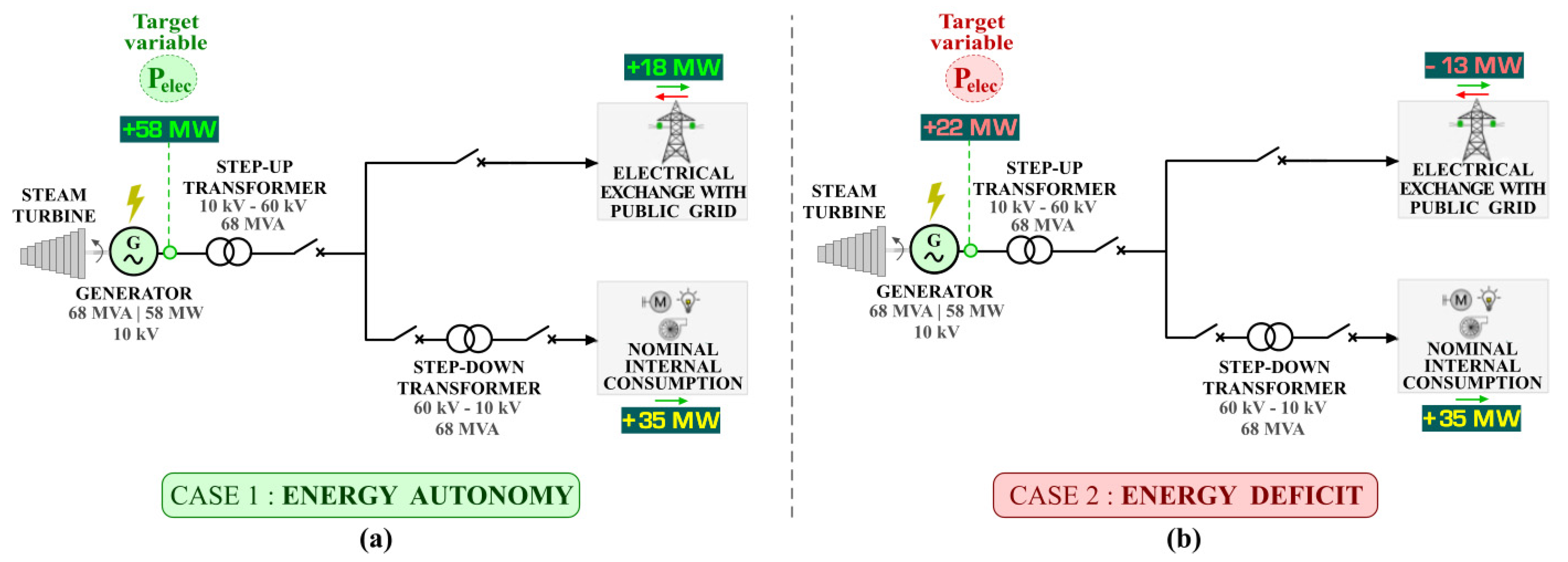
5.2. Implications of Findings
Given that 35 MW is the nominal consumption of the industrial unit, and as shown in
Figure 10, the energy exchanged between the self-produced electricity of the factory and the public electrical grid plays a dual role:
- (a)
It can inject and sell supplementary energy to the external electrical grid when the produced power exceeds the internal nominal consumption;
- (b)
It provides the possibility for the industrial unit to obtain electricity during periods when its thermal power plant does not cover local self–supply, i.e., when it is in deficit.
For this type electrical energy deficit problem, there is a need to predict the power produced since in this case, the industrial unit will have to buy electricity, impacting its energy bill.
In other words, the prediction of the target parameter
Pelec can allow industrial operators to act upstream at the right time on the processing parameters described in
Table 2, primarily when the power produced is likely to decrease to under 35 MW.
6. Conclusions and Perspectives
This study showed that the hybrid CNN-LSTM model was the most reliable algorithm, which made it possible to provide accurate and efficient predictions of the electrical power produced in the case of a steam power plant based on industrial exothermic reactions. This achievement implied an impact seen at two levels.
First, the prediction of the attenuation linked to the electrical power as the target parameter takes on an important anticipation characteristic, which can act as a decision-making tool for industrial managers. This is seen as being particularly important for ensuring the continuous and autonomous electrical feeding of industrial facilities.
Second, this prediction also aims to determine the input parameters that influence the decrease in the produced power. Thus, this prediction can provide the opportunity to instantly take action in the process in order to prevent the occurrence of prolonged undesirable variations in these input variables, that may force the end-user to import electricity for a long period of time.
In terms of perspective, it is now necessary to use Business Intelligence (BI) techniques to create a dynamic dashboard, which displays in real-time the measurement curve of electrical power superimposed on that of the prediction with a forecast horizon, as well as the real-time measurement of the input parameters to visualize and track their variations. As a result, helping decision makers to take the necessary actions at the right time can increase the profitability of industrial plants that self-produce electricity.
Author Contributions
Conceptualization, K.F.; Methodology, C.E. and M.E.M.; Software, K.F.; Validation, C.E. and M.E.M.; Formal analysis, K.F., C.E. and M.E.M.; Investigation, M.E.M. and C.E.; Resources, K.F., C.E. and M.E.M.; Data curation, K.F.; Writing—original draft preparation, K.F.; Writing—review and editing, K.F., C.E. and M.E.M.; Visualization, K.F., C.E. and M.E.M.; Supervision, C.E. and M.E.M.; Project administration, C.E. and M.E.M.; Funding acquisition, K.F. All authors have read and agreed to the published version of the manuscript.
Funding
This research received no external funding.
Data Availability Statement
Not applicable.
Conflicts of Interest
The authors declare no conflict of interest.
References
- Mansoor, K.; Tianqi, L.; Farhan, U. A New Hybrid Approach to Forecast Wind Power for Large Scale Wind Turbine Data Using Deep Learning with TensorFlow Framework and Principal Component Analysis. Energies 2019, 12, 2229. [Google Scholar]
- Dimitris, Z.; Georgios, T.; John, K. Forecasting of Wind Power Generation with the Use of Artificial Neural Networks and Support Vector Regression Models. In Proceedings of the Applied Energy Symposium and Forum, Renewable Energy Integration with Mini/Microgrids, Rhodes, Greece, 29–30 September 2018. [Google Scholar]
- Mohammed, S.; El Hassouni, M. A Novel Deep Learning Approach for Short Term Photovoltaic Power Forecasting Based on GRU-CNN Model. In E3S Web of Conferences; EDP Sciences: Les Ulis, France, 2022; Volume 336, p. 00064. [Google Scholar]
- Ahamed Saleel, C. Forecasting the energy output from a combined cycle thermal power plant using deep learning models. Case Stud. Therm. Eng. 2021, 28, 101693. [Google Scholar] [CrossRef]
- Maria, K.; Stefani, P.; Alexandros, G. Solar Photovoltaic Forecasting of Power Output Using LSTM Networks. Atmosphere 2021, 12, 124. [Google Scholar] [CrossRef]
- Ying, W.; Feng, B.; Qing-Song, H.; Sun, L. Short-Term Solar Power Forecasting: A Combined Long Short-Term Memory and Gaussian Process Regression Method. Sustainability 2021, 13, 3665. [Google Scholar]
- Azim, H.; Meysam Majidi, N.; Mehdi, N.; Davide Astiaso, G.; Farshid, K.; Livio, D.; Lina, B. A Combined Fuzzy GMDH Neural Network and Grey Wolf Optimization Application for Wind Turbine Power Production Forecasting Considering SCADA Data. Energies 2021, 14, 3459. [Google Scholar]
- Tianyang, L.; Zunkai, H.; Tian, L.; Yongxin, Z.; Wang, H.; Songlin, F. Enhancing Wind Turbine Power Forecast via Convolutional Neural Network. Electronics 2021, 10, 261. [Google Scholar] [CrossRef]
- Alrayess, H.; Asli, U. Forecasting the hydroelectric power generation of GCMs using machine learning techniques and deep learning (Almus Dam, Turkey). Geofizika 2021, 38, 1–90. [Google Scholar] [CrossRef]
- Paula, B.; Ahmad, T.; Qammer, H.; Basel, B. Solar Irradiance Forecasting Using a Data-Driven Algorithm and Contextual Optimisation. Appl. Sci. 2022, 12, 134. [Google Scholar]
- Weijie, Z.; Huihui, T.; Huimin, J. Application of a Novel Optimized Fractional Grey Holt-Winters Model in Energy Forecasting. Sustainability 2022, 14, 3118. [Google Scholar] [CrossRef]
- Shohan, M.; Faruque, M.; Simon, Y. Forecasting of Electric Load Using a Hybrid LSTM-Neural Prophet Model. Energies 2022, 15, 2158. [Google Scholar] [CrossRef]
- Elena, R.; Isabella, P.; Renato, I. Multilinear Regression Model for Biogas Production Prediction from Dry Anaerobic Digestion of OFMSW. Sustainability 2022, 14, 4393. [Google Scholar] [CrossRef]
- Dongyu, W.; Xiwen, C.; Dongxiao, N. Wind Power Forecasting Based on LSTM Improved by EMD-PCA-RF. Sustainability 2022, 14, 7307. [Google Scholar] [CrossRef]
- Xuan-Hien, L.; Hung, V.; Giha, L.; Sungho, J. Application of Long Short-Term Memory (LSTM) Neural Network for Flood Forecasting. Water 2019, 11, 1387. [Google Scholar] [CrossRef]
- Wang, J.; Zihao, L. Research on Face Recognition Based on CNN. In IOP Conference Series: Earth and Environmental Science, Proceedings of the 2nd International Symposium on Resource Exploration and Environmental Science, Ordos, China, 28–29 April 2018; IOP Publishing Ltd.: Bristol, UK, 2018; Volume 170, p. 170. [Google Scholar]
- Rahim, B.; Taghi Aalami, M.; Adamowski, J. Short-term water quality variable prediction using a hybrid CNN–LSTM deep learning model. Stoch. Environ. Res. Risk Assess. 2020, 34, 415–433. [Google Scholar]
- Reddy, P.C.; Sureshbabu, A. An Adaptive Model for Forecasting Seasonal Rainfall Using Predictive Analytics. Int. J. Intell. Eng. Syst. 2019, 12, 22–32. [Google Scholar] [CrossRef]
- Saengmuang, A.; Sitjongsataporn, S. Convergence and Stability Analysis of Spline Adaptive Filtering based on Adaptive Averaging Step-size Normalized Least Mean Square Algorithm. Int. J. Intell. Eng. Syst. 2020, 13, 267–277. [Google Scholar]
- Loverude, M.E.; Kautz, C.H.; Paula, R.L. Heron: Student understanding of the first law of thermodynamics: Relating work to the adiabatic compression of an ideal gas. Am. J. Phys. 2002, 70, 137. [Google Scholar] [CrossRef]
- Onwuamaeze, P.I. Improving steam turbine efficiency: An appraisal. Res. J. Mech. Oper. 2018, 1, 24–30. [Google Scholar]
| Publisher’s Note: MDPI stays neutral with regard to jurisdictional claims in published maps and institutional affiliations. |
© 2022 by the authors. Licensee MDPI, Basel, Switzerland. This article is an open access article distributed under the terms and conditions of the Creative Commons Attribution (CC BY) license (https://creativecommons.org/licenses/by/4.0/).


