
Identifying Past Remains of Morphologically Similar Vole Species Using Molar Shapes

 ,
,
Abstract
1. Introduction
2. Material and Methods
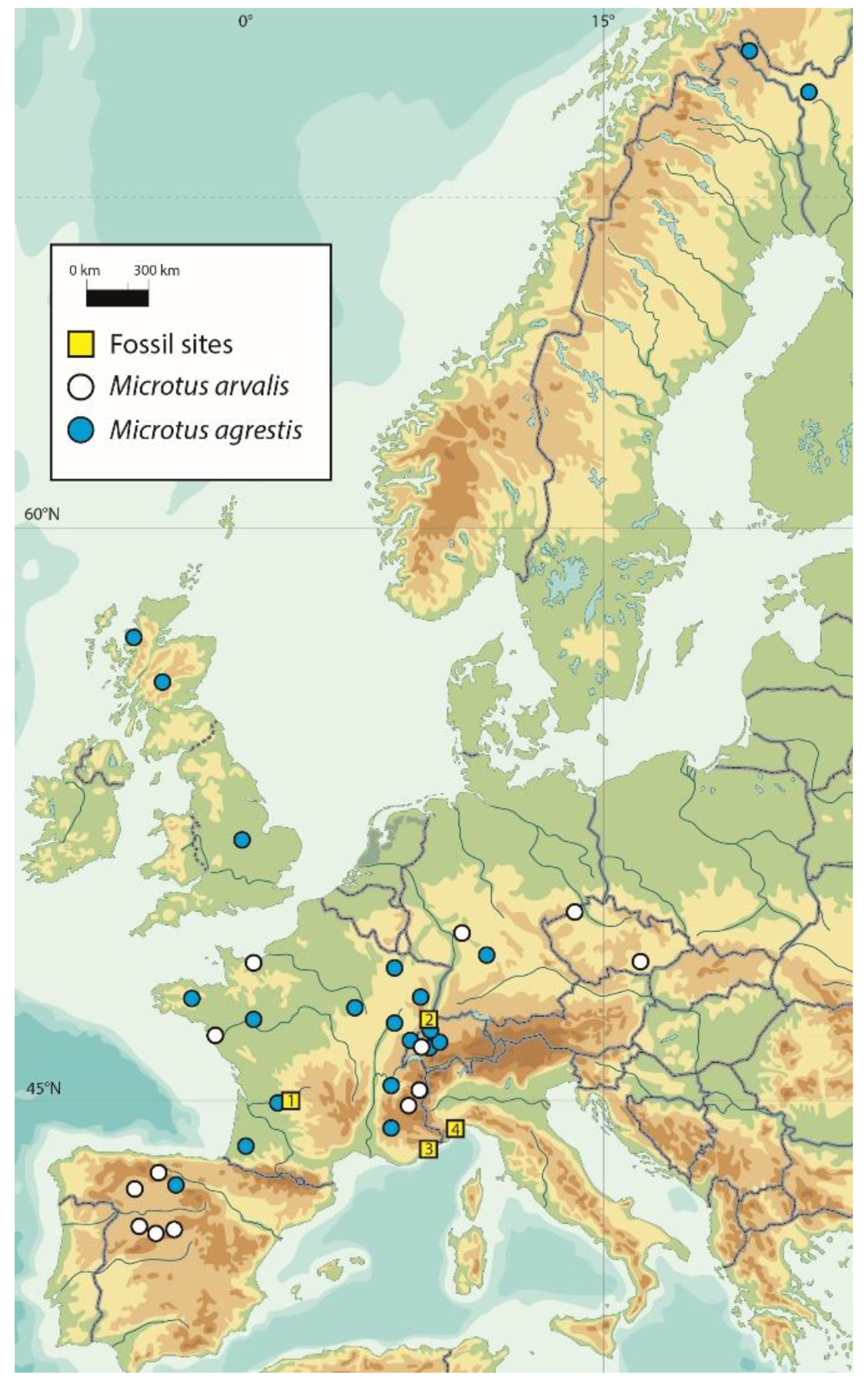
2.1. Modern Samples
2.2. Fossil Material Remains
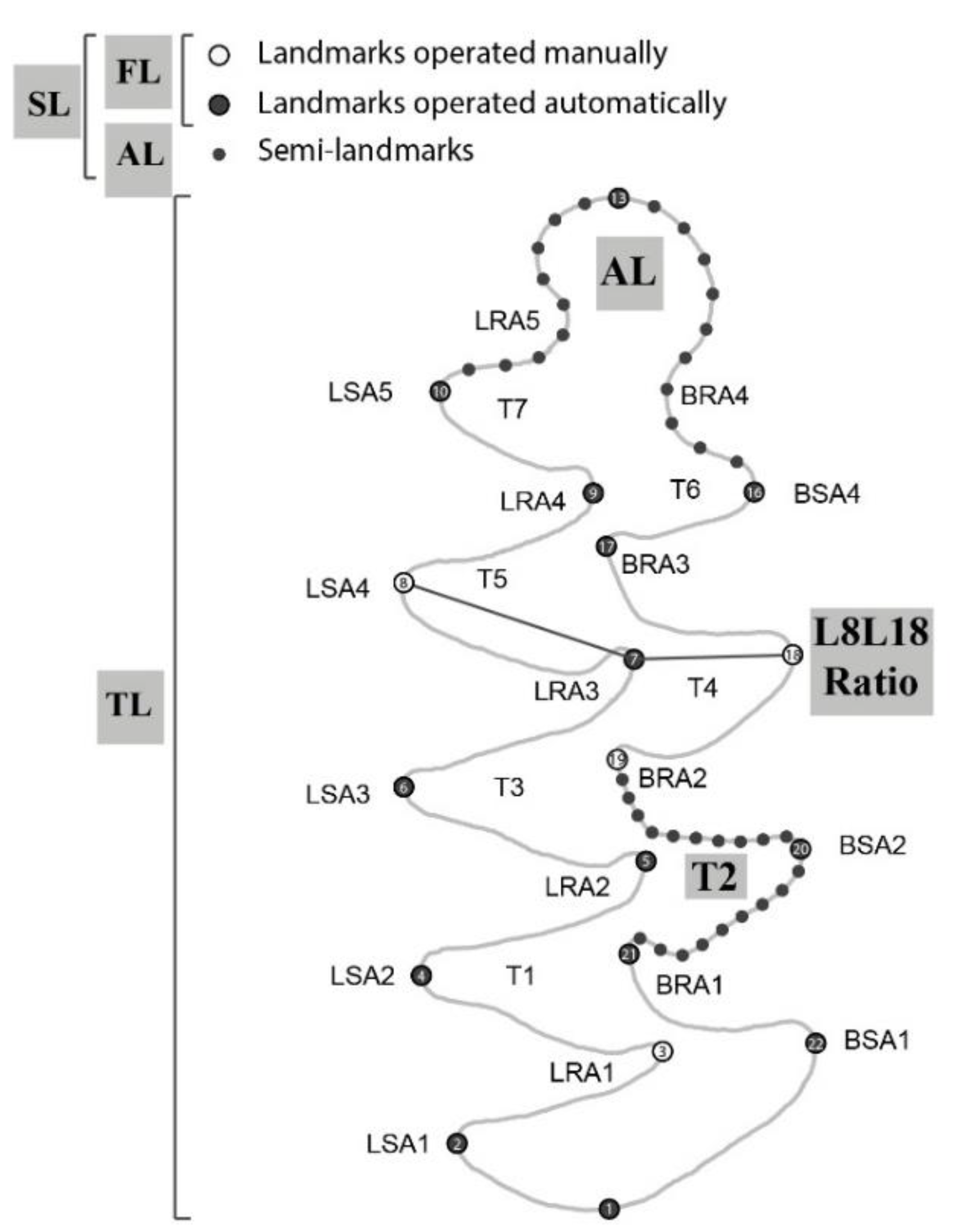
2.3. Landmark Schemes and Digitization
2.4. Geometric Morphometrics
2.5. Statistical Classification
3. Results
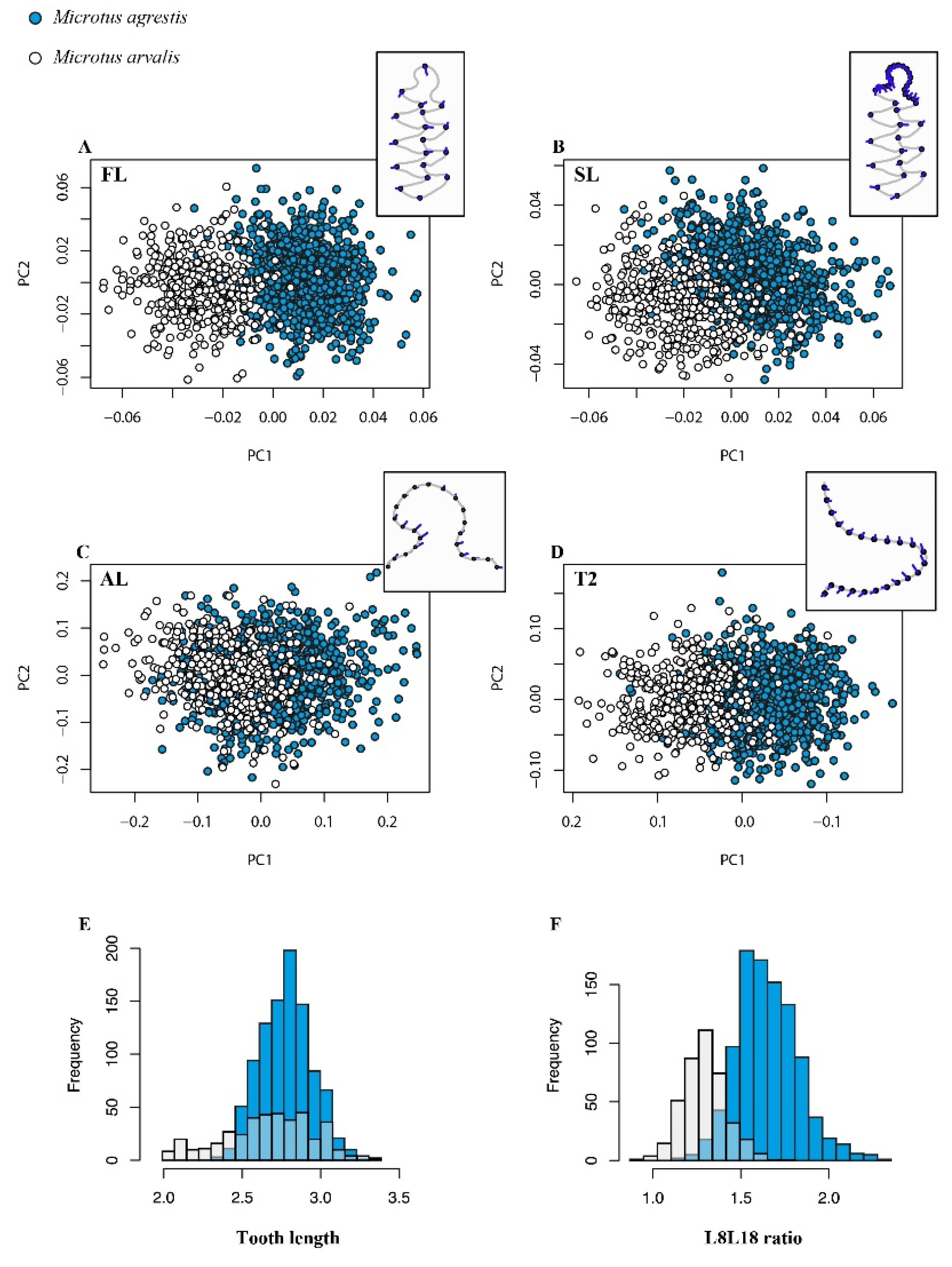
3.1. Morphospaces
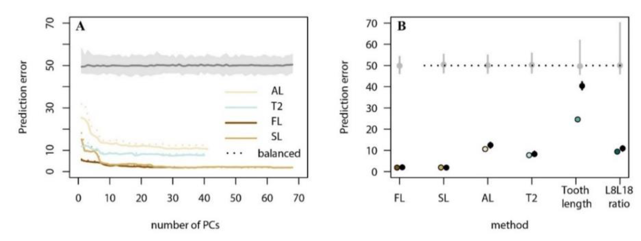
3.2. Present-Day Model Training and Evaluation
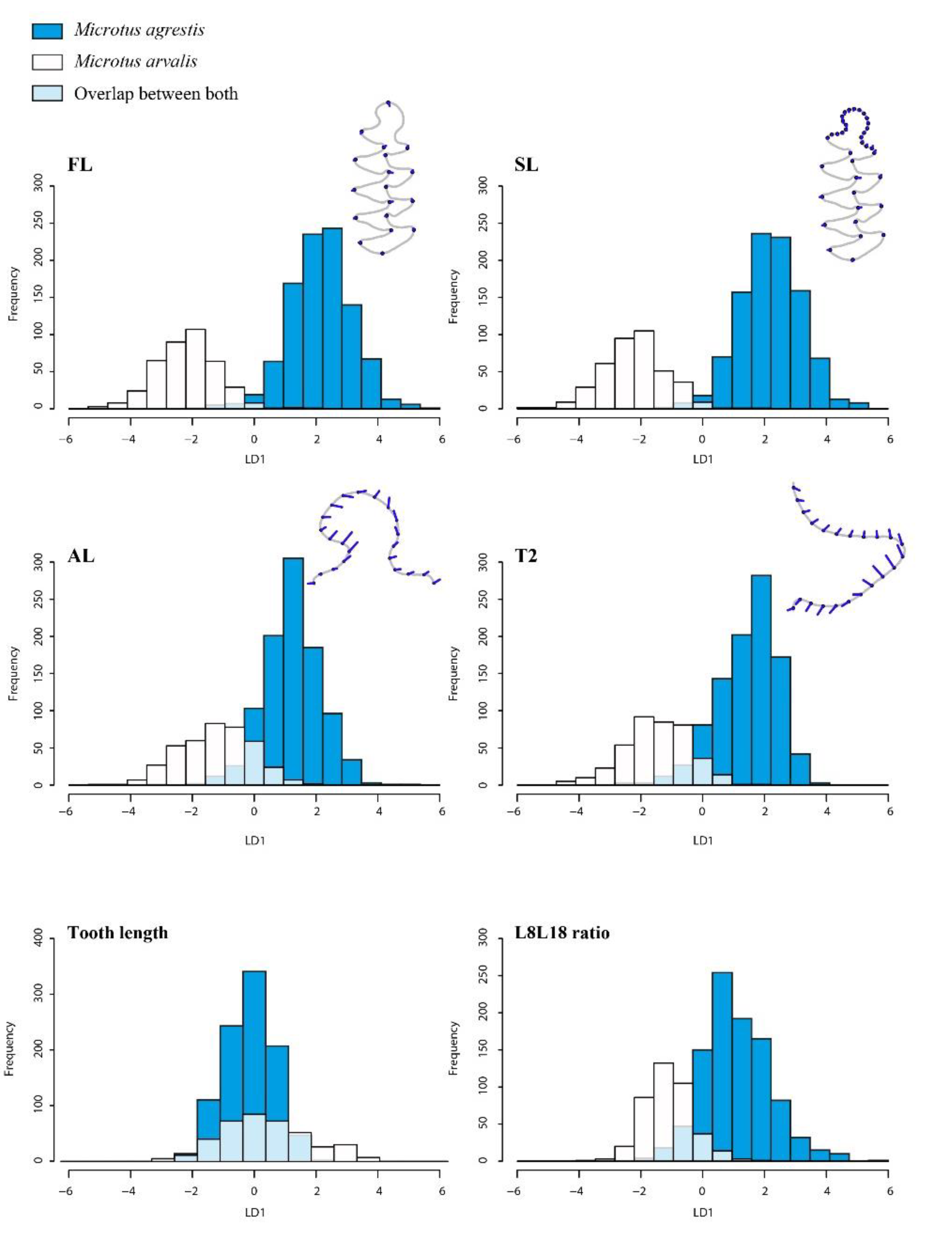
3.2.1. The Arvalis-Agrestis Differentiation
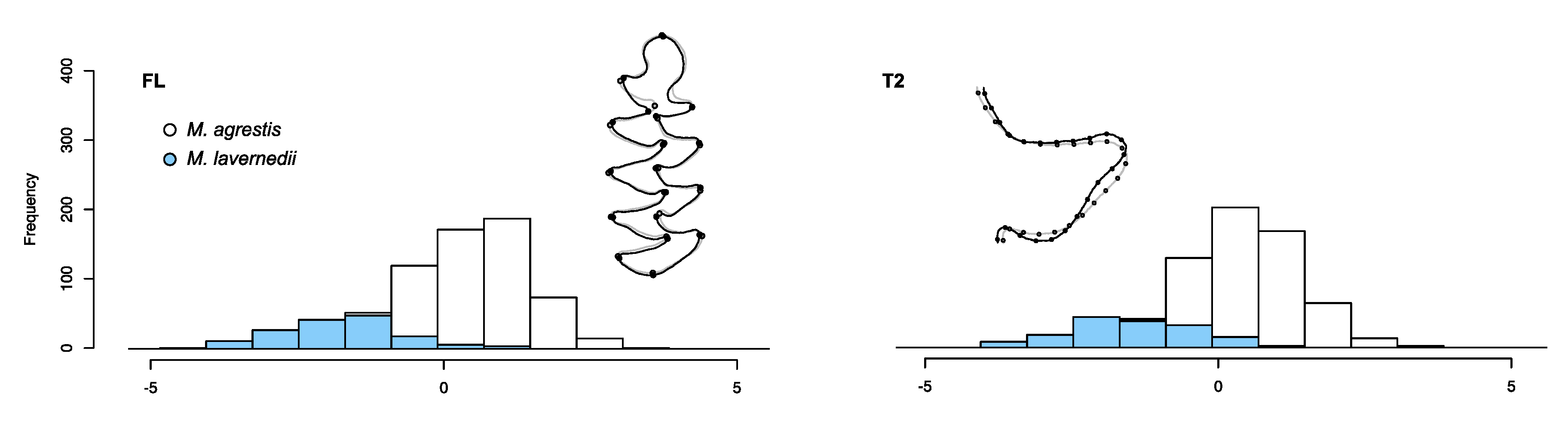
3.2.2. Identifying Variants within the Field Vole
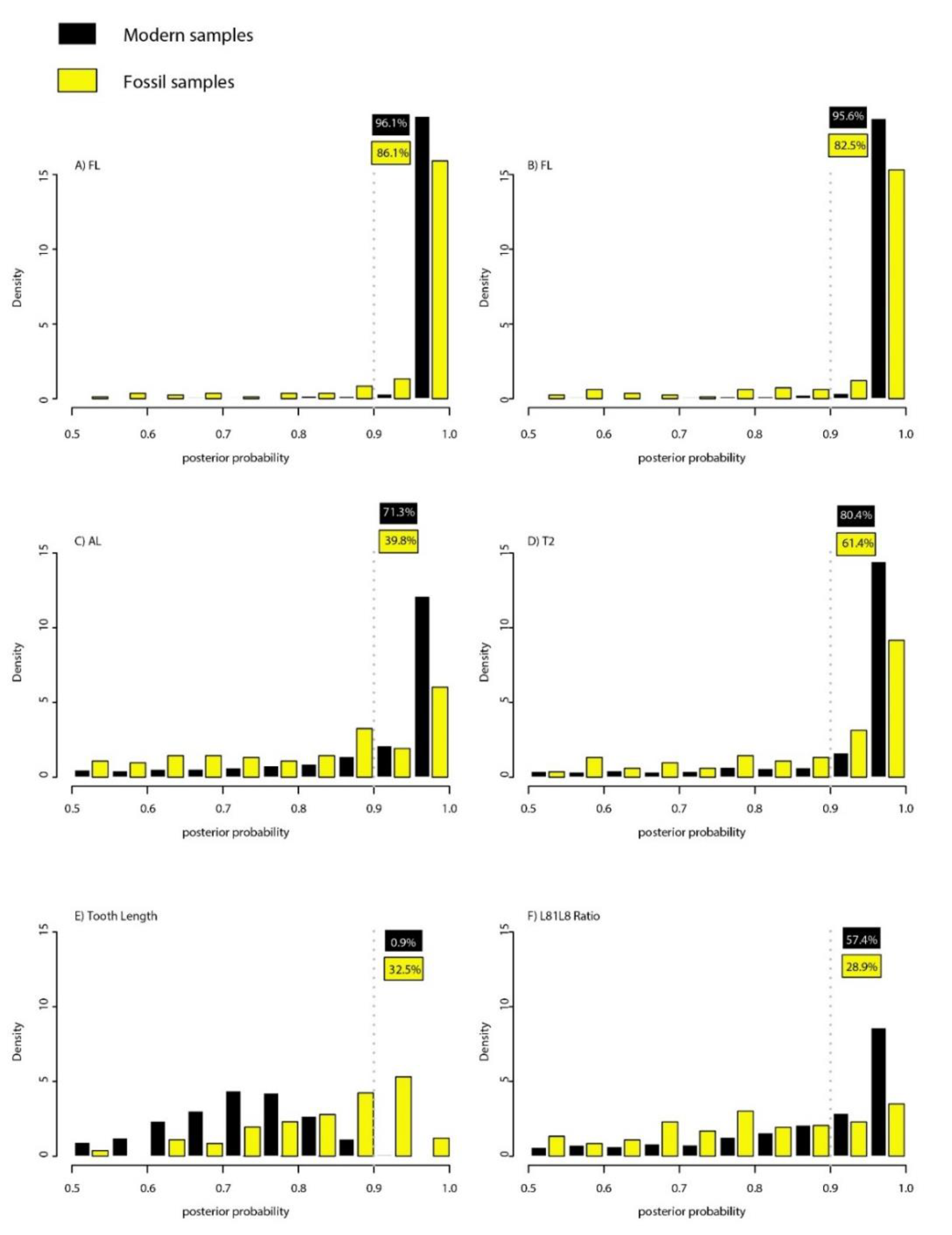
3.3. Statistical Fossil Identification
4. Discussion
4.1. Molar Shape Variations and Discriminant Models
4.2. Fossil Variations and Their Implications
Supplementary Materials
Author Contributions
Funding
Acknowledgments
Conflicts of Interest
References
- Krapp, F.J.; Niethammer, J. Microtus agrestis (Linnaeus. 1761)-Erdmaus. In Handbuch der Säugetiere Europas: Nagetiere II; Niethammer, J., Krapp, F., Eds.; Akademische Verlagsgesellschaft: Wiesbaden, Germany, 1982; pp. 349–373. [Google Scholar]
- Dienske, H. The importance of social interactions and habitat in competition between Microtus agrestis and M. Arvalis. Behaviour 1979, 71, 1–125. [Google Scholar] [CrossRef]
- Quéré, J.P.; Le Louarn, H. Les Rongeurs de France: Faunistique et biologie—3e Edition Revue et Augmentée; Quae: Versailles, France, 2011. [Google Scholar]
- Wilson, D.E.; Lacher, T.E., Jr.; Mittermeir, R.A. Handbook of the Mammals of the World 7; Rodents II; Lynx Editions: Barcelona, Spain, 2017. [Google Scholar]
- Jaarola, M.; Martínková, N.; Gündüz, İ.; Brunhoff, C.; Zima, J.; Nadachowski, A.; Amori, G.; Bulatova, N.S.; Chondropoulos, B.; Fraguedakis-Tsolis, S. Molecular phylogeny of the speciose vole genus Microtus (Arvicolinae. Rodentia) inferred from mitochondrial DNA sequences. Mol. Phylogenet. Evol. 2004, 33, 647–663. [Google Scholar] [CrossRef] [PubMed]
- Barbosa, S.; Paupério, J.; Pavlova, S.V.; Alves, P.C.; Searle, J.B. The Microtus voles: Resolving the phylogeny of one of the most speciose mammalian genera using genomics. Mol. Phylogenet. Evol. 2018, 125, 85–92. [Google Scholar] [CrossRef] [PubMed]
- Hinton, M.A.C. Monograph of the Voles and Lemmings (Microtinae) Living and Extinct; Natural History Museum: London, UK, 1926; p. 488. [Google Scholar]
- Vinogradov, B.S.; Argiropulo, A.I. Fauna of the USSR. Key to Rodents; IPST: Jerusalem, Israel, 1941. [Google Scholar]
- Dienske, H. Notes on differences between some external and skull characters of Microtus arvalis (Pallas. 1778) and of Microtus agrestis (Linnaeus, 1761) from the Netherlands. Zool. Meded. 1969, 44, 83–108. [Google Scholar]
- Fedyk, A.; Ruprecht, A.L. Taxonomic value of M1 measurements in Microtus agrestis (Linnaeus. 1761) and Microtus arvalis (Pallas, 1779). Acta Theriol. 1971, 16, 408–412. [Google Scholar] [CrossRef]
- Chaline, J. Les Rongeurs du Pléistocène Moyen et Supérieur de France; Editions du Centre National de la Recherche Scientifique: Paris, France, 1972. [Google Scholar]
- Nadachowski, A. Taxonomic value of anteroconid measurements of M1 in common and field voles. Acta Theriol. 1984, 29, 123–127. [Google Scholar] [CrossRef]
- Reiner, G. Eine spätglaziale Mikrovertebratenfauna aus der Grossen Badhöhle bei Peggau. Steiermark. Mitt Abt Geol Paläont Landesmus Joanneum 1995, 52–53, 135–192. [Google Scholar]
- Abbassi, M. Essai de différenciation entre Microtus arvalis et Microtus agrestis à partir de l’étude de quatre populations fossiles (Sud-Est de la France et Ligurie italienne). Bulletin du Musée d’Anthropologie Préhistorique de Monaco 1997, 39, 45–51. [Google Scholar]
- Van Der Kooij, J.; Gillham, M.; Post, R.J.; Heijerman, T.; Wilson, M.D. Morphometric variation in the mandible of Microtus arvalis and Microtus agrestis (Rodentia: Cricetidae). Neth. J. Zool. 1997, 47, 47–59. [Google Scholar] [CrossRef]
- Navarro, N.; Zatarain, X.; Montuire, S. Effects of morphometric descriptor changes on statistical classification and morphospaces. Boil. J. Linn. Soc. 2004, 83, 243–260. [Google Scholar] [CrossRef]
- Markova, E.A.; Borodin, A.V. Species identification of voles (subgenus Microtus Schrank. 1798) from the Urals and Western Siberia through the first lower molar measurements. In Ural and Siberia Faunas at Pleistocene and Holocene Times; Biota of Northern Eurasia in Cenozoic Series 4; Institute of Plant and Animal Ecology, Ural Branch of Russian Academy of Sciences: Chelyabinsk, Russia, 2005; pp. 3–10. (In Russian) [Google Scholar]
- Ivanov, D.L. Идентификация Microtus agrestis L. и Microtus ex gr. arvalis Pall. в ископаемых фаунах голоцена Беларуси. Вестник 2008, 1, 87–93. [Google Scholar]
- Luzi, E.; López-García, J.M.; Blasco, R.; Rivals, F.; Rosell, J. Variations in Microtus arvalis and Microtus agrestis (Arvicolinae. Rodentia) dental morphologies in an archaeological context: The case of Teixoneres Cave (Late Pleistocene, North-Eastern Iberia). J. Mamm. Evol. 2017, 24, 495–503. [Google Scholar] [CrossRef]
- Zannotti, S. Morphometric analysis on M1 to determine subfossilspecimens of Microtus arvalis (Pallas. 1778) and Microtus agrestis (Linnaeus,1761) from North- Eastern Italy. Bollettino del Museo Civico di Storia Naturale di Verona 2016, 40, 37–51. [Google Scholar]
- Barkaszi, Z. Diagnostic Criteria for Identification of Microtus s.l. Species (Rodentia. Arvicolidae) of the Ukrainian Carpathians. Vestnik Zool. 2017, 51, 471–486. [Google Scholar] [CrossRef]
- Blasius, J.H. Naturgeschichte der Säugethiere Deutschlands und der Angrenzenden Länder von Mitteleuropa; F. Vieweg und Sohn: Berlin, Germany, 1857; Volume 1. [Google Scholar]
- Reichstein, H.; Reise, D. Zur Variabilität des Molaren-Schmelzschlingenmusters der Erdmaus. Microtus agrestis (L.). Zeitschrift für Säugetierkunde 1965, 30, 36–47. [Google Scholar]
- Van der Meulen, A.J. Middle Pleistocene smaller mammals from the Monte Peglia (Orvieto. Italy) with special reference to the phylogeny of Microtus (Arvicolidae, Rodentia). Quaternaria 1973, 17, 1–144. [Google Scholar]
- Brunet-Lecomte, P. Les Campagnols Souterrains, Terricola, Arvicolidae, Rodentia, Actuels et Fossiles d’Europe Occidentale. Ph.D. Thesis, Université de Bourgogne, Dijon, France, 1988. [Google Scholar]
- Laplana, C.; Montuire, S.; Brunet-Lecomte, P.; Chaline, J. Révision des Allophaiomys (Arvicolinae. Rodentia, Mammalia) des Valerots (Côte-d’Or, France). Geodiversitas 2000, 22, 255–267. [Google Scholar]
- Luzi, E.; López-García, J.M. Patterns of variation in Microtus arvalis and Microtus agrestis populations from Middle to Late Pleistocene in southwestern Europe. Hist. Biol. 2017, 1, 1–9. [Google Scholar] [CrossRef]
- Brunet-Lecomte, P.; Nadachowski, A.; Sirugue, D.; Indelicato, N. À propos de l’observation d’un rhombe pitymyen à la première molaire inférieure chez les campagnols Microtus arvalis et M. agrestis (Rodentia. Arvicolidae). Mammalia 1996, 60, 491–495. [Google Scholar] [CrossRef]
- Brunet-Lecomte, P. A propos de l’observation de cas de campagnols des champs Microtus arvalis (Pallas. 1778) (Rodentia, Arvicolinae) caractérisés par une première molaire inférieure présentant un rhombe pitymyen. Bulletin Mensuel de la Société Linnéenne de Lyon 2008, 77, 41–43. [Google Scholar] [CrossRef]
- Kowalski, K. Variations and speciation of fossil voles. Mammal Rev. 1970, 1, 36. [Google Scholar] [CrossRef]
- Jaarola, M.; Searle, J.B. A highly divergent mitochondrial DNA lineage of Microtus agrestis in Southern Europe. Heredity 2004, 92, 228–234. [Google Scholar] [CrossRef] [PubMed]
- Paupério, J.; Herman, J.S.; Melo-Ferreira, J.; Jaarola, M.; Alves, P.C.; Searle, J.B. Cryptic speciation in the field vole: A multilocus approach confirms three highly divergent lineages in Eurasia. Mol. Ecol. 2012, 21, 6015–6032. [Google Scholar] [CrossRef] [PubMed]
- Beysard, M.; Perrin, N.; Jaarola, M.; Heckel, G.; Vogel, P. Asymmetric and differential gene introgression at a contact zone between two highly divergent lineages of field voles (Microtus agrestis). J. Evol. Boil. 2012, 25, 400–408. [Google Scholar] [CrossRef] [PubMed]
- Patton, J.L. Family Cricetidae (true hamsters, voles, lemmings and new world rats and mice). Species accounts of Cricetidae. In Handbook of the Mammals of the World 7; Rodents II; Wilson, D.E., Lacher, T.E., Jr., Mittermeier, R.A., Eds.; Lynx Editions: Barcelona, Spain, 2017; Volume 7, pp. 321–334. [Google Scholar]
- Langlais, M.; Laroulandie, V.; Bruxelles, L.; Chalard, P.; Cochard, D.; Costamagno, S.; Delfour, G.; Kuntz, D.; Le Gall, O.; Pétillon, J.-M. Les fouilles de la grotte-abri de Peyrazet (Creysse, Lot): Nouvelles données pour le Tardiglaciaire quercinois. Bulletin de la SOCIETE Préhistorique Française 2009, 106, 150–152. [Google Scholar] [CrossRef]
- Langlais, M.; Laroulandie, V.; Jacquier, J.; Costamagno, S.; Chalard, P.; Mallye, J.-B.; Pétillon, J.-M.; Rigaud, S.; Royer, A.; Sitzia, L. Le Laborien récent de la grotte-abri de Peyrazet (Creysse, Lot). Nouvelles données pour la fin du Tardiglaciaire en Quercy. Paléo 2015, 26, 79–116. [Google Scholar]
- Royer, A. How complex is the evolution of small mammal communities during the Late Glacial in southwest France? Quat. Int. 2016, 414, 23–33. [Google Scholar] [CrossRef]
- Koehler, H.; Angevin, R.; Bignon-Lau, O.; Griselin, S. Découverte de plusieurs occupations du Paléolithique supérieur récent dans le Sud de l’Alsace. Bulletin de la Société Préhistorique Française 2013, 110, 356–359. [Google Scholar] [CrossRef]
- Abbassi, M. Les Rongeurs du Sud-Est de la France et de Ligurie: Implications Systématiques. Ph.D. Thesis, Muséum National D’histoire Naturelle, Paris, France, 1999. [Google Scholar]
- Dryden, I.L.; Mardia, K.V. Statistical Shape Analysis; Wiley: Chichester, UK, 1998; p. 347. [Google Scholar]
- Bookstein, F.L. Landmark methods for forms without landmarks: Morphometrics of group differences in outline shape. Med. Image Anal. 1997, 1, 225–243. [Google Scholar] [CrossRef]
- Adams, D.C.; Otárola-Castillo, E. geomorph: An R package for the collection and analysis of geometric morphometric shape data. Methods Ecol. Evol. 2013, 4, 393–399. [Google Scholar] [CrossRef]
- Hastie, T.; Tibshirani, R.; Friedman, J. The Elements of Statistical Learning, 2nd ed.; Springer: New York, NY, USA, 2009; p. 745. [Google Scholar]
- Evin, A.; Cucchi, T.; Cardini, A.; Vidarsdottir, U.S.; Larson, G.; Dobney, K. The long and winding road: Identifying pig domestication through molar size and shape. J. Archaeol. Sci. 2013, 40, 735–743. [Google Scholar] [CrossRef]
- Searle, J.B.; Kotlík, P.; Rambau, R.V.; Markova, S.; Herman, J.S.; McDevitt, A.D. The Celtic fringe of Britain: Insights from small mammal phylogeography. Proc. R. Soc. B 2009, 276, 4287–4294. [Google Scholar] [CrossRef] [PubMed]
- Brace, S.; Palkopoulou, E.; Dalén, L.; Lister, A.M.; Miller, R.; Otte, M.; Germonpré, M.; Blockley, S.P.; Barnes, I. Serial population extinctions in a small mammal indicate Late Pleistocene ecosystem instability. Proc. Natl. Acad. Sci. USA 2012, 109, 20532–20536. [Google Scholar] [CrossRef] [PubMed]
- Brace, S.; Ruddy, M.; Miller, R.; Schreve, D.C.; Stewart, J.R.; Barnes, I. The colonization history of British water vole (Arvicola amphibius (Linnaeus. 1758)): Origins and development of the Celtic fringe. Proc. R. Soc. B. 2016, 283, 20160130. [Google Scholar] [CrossRef] [PubMed]
- Baca, M.; Nadachowski, A.; Lipecki, G.; Mackiewicz, P.; Marciszak, A.; Popović, D.; Socha, P.; Stefaniak, K.; Wojtal, P. Impact of climatic changes in the Late Pleistocene on migrations and extinction of mammals in Europe: Four case studies. Geol. Q. 2017, 61, 291–304. [Google Scholar]
- Maul, L. Üeberblick über die unterpleistozänen Kleinsäugerfaunen Europas. Quartärpaläontologie 1990, 8, 153–191. [Google Scholar]
- Kowalski, K. Pleistocene rodents of Europe. Folia Quat. 2001, 72, 3–389. [Google Scholar]
- Kolfschoten, T.V.; Turner, E. Early Middle Pleistocene mammalian faunas from Kärlich and Miesenheim I and their biostratigraphical implications. In The Early Middle Pleistocene in Europe; Balkerna: Rotterdam, The Netherlands, 1996; pp. 227–253. [Google Scholar]
- Jeannet, M. Les Rongeurs d’Orgnac 3 (Ardèche) DES Sciences Naturelles; Sciences de la Terre, Université de Dijon: Dijon, France, 1974. [Google Scholar]
- Jánossy, D. Pleistocene Vertebrate Faunas of Hungary; Elsevier: New York, NY, USA, 1986. [Google Scholar]
- López Antoñanzas, R.; Bescós, G.C. The Gran Dolina site (Lower to Middle Pleistocene. Atapuerca, Burgos, Spain): New palaeoenvironmental data based on the distribution of small mammals. Palaeogeogr. Palaeoclimatol. Palaeoecol. 2002, 186, 311–334. [Google Scholar]
- Herman, J.S.; Searle, J.B. Post-glacial partitioning of mitochondrial genetic variation in the field vole. Proc. R. Soc. B 2011, 278, 3601–3607. [Google Scholar] [CrossRef] [PubMed]
- Tougard, C.; Renvoisé, E.; Petitjean, A.; Quéré, J. New insight into the colonization processes of common voles: Inferences from molecular and fossil evidence. PLoS ONE 2008, 3, e3532. [Google Scholar] [CrossRef] [PubMed]
- Herman, J.S.; McDevitt, A.D.; Kawałko, A.; Jaarola, M.; Wójcik, J.M.; Searle, J.B. Land-bridge calibration of molecular clocks and the post-glacial colonization of Scandinavia by the Eurasian field vole Microtus agrestis. PLoS ONE 2014, 9, e103949. [Google Scholar] [CrossRef] [PubMed]


| Localities | Region | Species1 | Number of Teeth | |
|---|---|---|---|---|
| Modern samples | Drnholec | Czech Republic | Microtus arvalis | 25 |
| Krušné hory | Czech Republic | Microtus arvalis | 23 | |
| Parc national de la Vanoise | France | Microtus arvalis | 24 | |
| Caen (Normandie) | France | Microtus arvalis | 60 | |
| Noirmoutier | France | Microtus arvalis | 34 | |
| Monetier-les-Bains | France | Microtus arvalis | 26 | |
| La Hesse | Germany | Microtus arvalis | 55 | |
| Lomilla + Urbe | Spain | Microtus arvalis | 18 | |
| Luengos + Mayorga + Villaloba | Spain | Microtus arvalis | 18 | |
| Ledesma + Bocigas | Spain | Microtus arvalis | 17 | |
| Yangus | Spain | Microtus arvalis | 16 | |
| Carbones | Spain | Microtus arvalis | 62 | |
| Joux + Mont Tendre + Verrieres | Switzerland | Microtus arvalis | 24 | |
| Southern part of England | England | Microtus agrestis | 30 | |
| Pallasjärvi | Finland | Microtus agrestis | 66 | |
| Kilpisjärvi | Finland | Microtus agrestis | 92 | |
| Côte d’Or | France | Microtus agrestis | 66 | |
| Meuse | France | Microtus agrestis | 33 | |
| Chabons (Isère) | France | M. agrestis/uncertain | 76 | |
| Dordogne | France | M. agrestis/lavernedii | 84 | |
| Alpes Haute Provence | France | M. agrestis/uncertain | 22 | |
| Grandchamp (Yonne) | France | Microtus agrestis | 90 | |
| Saint-Aignan (Bretagne) | France | Microtus agrestis | 42 | |
| Longué-Jumelles (Maine-et-Loire) | France | M. agrestis/uncertain | 55 | |
| South of Landes + France part of Basque Country | France | M. agrestis/lavernedii | 15 | |
| Rupt-sur-Moselle (Vosges) | France | Microtus agrestis | 17 | |
| Bavaria + La Hesse | Germany | Microtus agrestis | 61 | |
| Northwestern part of Scotland | Scotland | Microtus agrestis | 33 | |
| Northern part of Scotland | Scotland | Microtus agrestis | 29 | |
| Burgos | Spain | Microtus agrestis | 15 | |
| Champery | Switzerland | M. agrestis/lavernedii | 28 | |
| Cheserex | Switzerland | M. agrestis/uncertain | 22 | |
| Seleute + Saint-Ursanne | Switzerland | Microtus agrestis | 82 | |
| Sion | Switzerland | M. agrestis/lavernedii | 15 | |
| Fossil samples | Peyrazet (Lot) | France | Microtus arvalis | 98 |
| Blénien Cave (Alsace) | France | Microtus agrestis | 22 | |
| Lazaret Cave (Alpes-Maritimes) | France | Microtus agrestis | 18 | |
| Arma delle Manie (Liguria) | Italy | Microtus agrestis | 28 |
| Model | Prediction Error (%) 1 | % (Posterior Probability > 0.9) 2 |
|---|---|---|
| FL | 1.89 | 96.1 |
| SL | 1.97 | 95.6 |
| AL | 10.64 | 71.3 |
| T2 | 7.73 | 80.4 |
| Tooth Length | 24.56 | 0.9 |
| L8L18 Ratio | 9.40 | 57.4 |
| Expert | FL | SL | AL | T2 | Tooth Length | L8L18 Ratio | ||
|---|---|---|---|---|---|---|---|---|
| Arma delle Manie | M. agrestis | 28 | 7 (4) | 8 (7 | 11 (6) | 15 (8) | 28 (0) | 14 (5) |
| M. arvalis | 0 | 21 (16) | 20 (17) | 17 (8) | 13 (7) | 0 | 14 (1) | |
| Lazaret | M. agrestis | 18 | 7 (4) | 10 (6) | 9 (5) | 14 (7) | 18 (0) | 11 (6) |
| M. arvalis | 0 | 11 (7) | 8 (8) | 9 (0) | 4 (1) | 0 | 7 (2) | |
| Blénien | M. agrestis | 22 | 22 (22) | 22 (21) | 19 (17) | 18 (15) | 22 (4) | 20 (14) |
| M. arvalis | 0 | 0 | 0 | 3 (1) | 4 (0) | 0 | 2 (0) | |
| Peyrazet | M. agrestis | 0 | 9 (4) | 17 (9) | 39 (10) | 15 (2) | 98 (50) | 39 (7) |
| M. arvalis | 98 | 89 (86) | 81 (72) | 59 (19) | 83 (63) | 0 | 59 (13) |
© 2018 by the authors. Licensee MDPI, Basel, Switzerland. This article is an open access article distributed under the terms and conditions of the Creative Commons Attribution (CC BY) license (http://creativecommons.org/licenses/by/4.0/).
Share and Cite
Navarro, N.; Montuire, S.; Laffont, R.; Steimetz, E.; Onofrei, C.; Royer, A. Identifying Past Remains of Morphologically Similar Vole Species Using Molar Shapes. Quaternary 2018, 1, 20. https://doi.org/10.3390/quat1030020
Navarro N, Montuire S, Laffont R, Steimetz E, Onofrei C, Royer A. Identifying Past Remains of Morphologically Similar Vole Species Using Molar Shapes. Quaternary. 2018; 1(3):20. https://doi.org/10.3390/quat1030020
Chicago/Turabian StyleNavarro, Nicolas, Sophie Montuire, Rémi Laffont, Emilie Steimetz, Catalina Onofrei, and Aurélien Royer. 2018. "Identifying Past Remains of Morphologically Similar Vole Species Using Molar Shapes" Quaternary 1, no. 3: 20. https://doi.org/10.3390/quat1030020
APA StyleNavarro, N., Montuire, S., Laffont, R., Steimetz, E., Onofrei, C., & Royer, A. (2018). Identifying Past Remains of Morphologically Similar Vole Species Using Molar Shapes. Quaternary, 1(3), 20. https://doi.org/10.3390/quat1030020