
Monitoring Coastal Waves with ICESat-2


Abstract
:1. Introduction
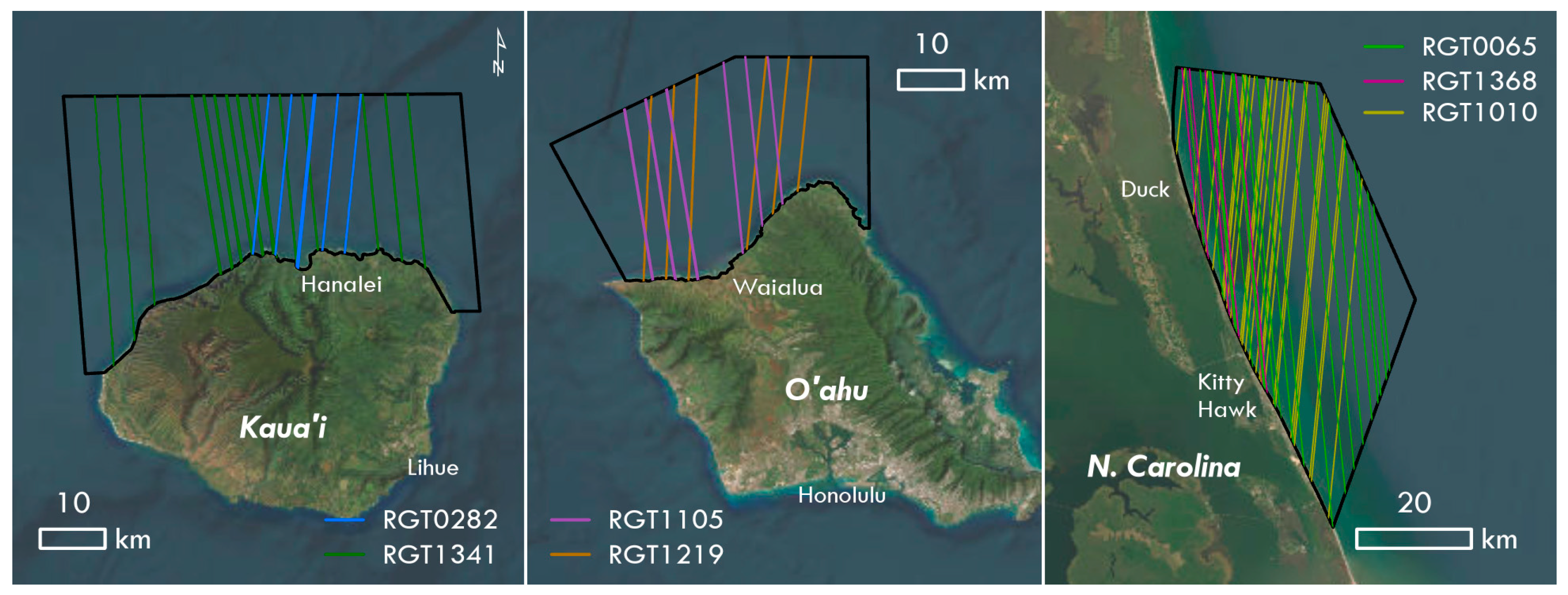
Study Area
2. Materials and Methods
2.1. ICESat-2 Background
2.2. Datasets
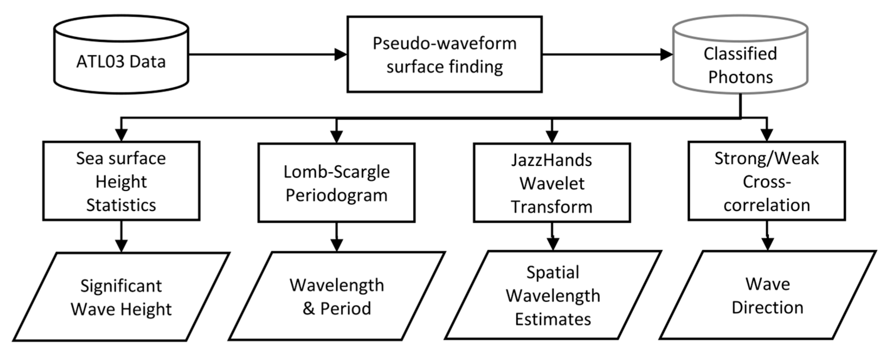
2.3. ATL03 Preprocessing
2.4. Basic Wave Metrics
2.5. Spatial Wave Metrics
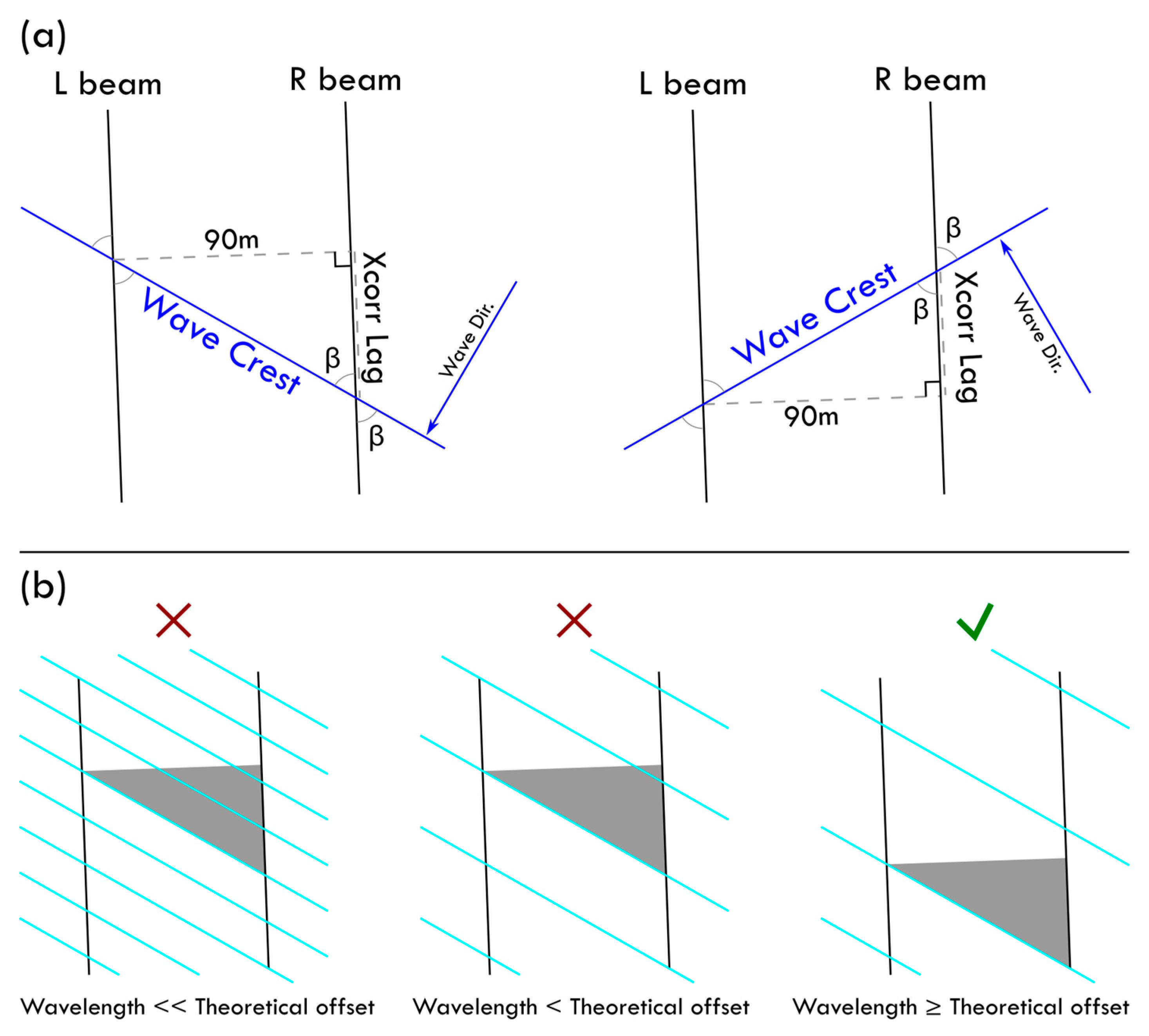
2.6. Wave Directionality
3. Results
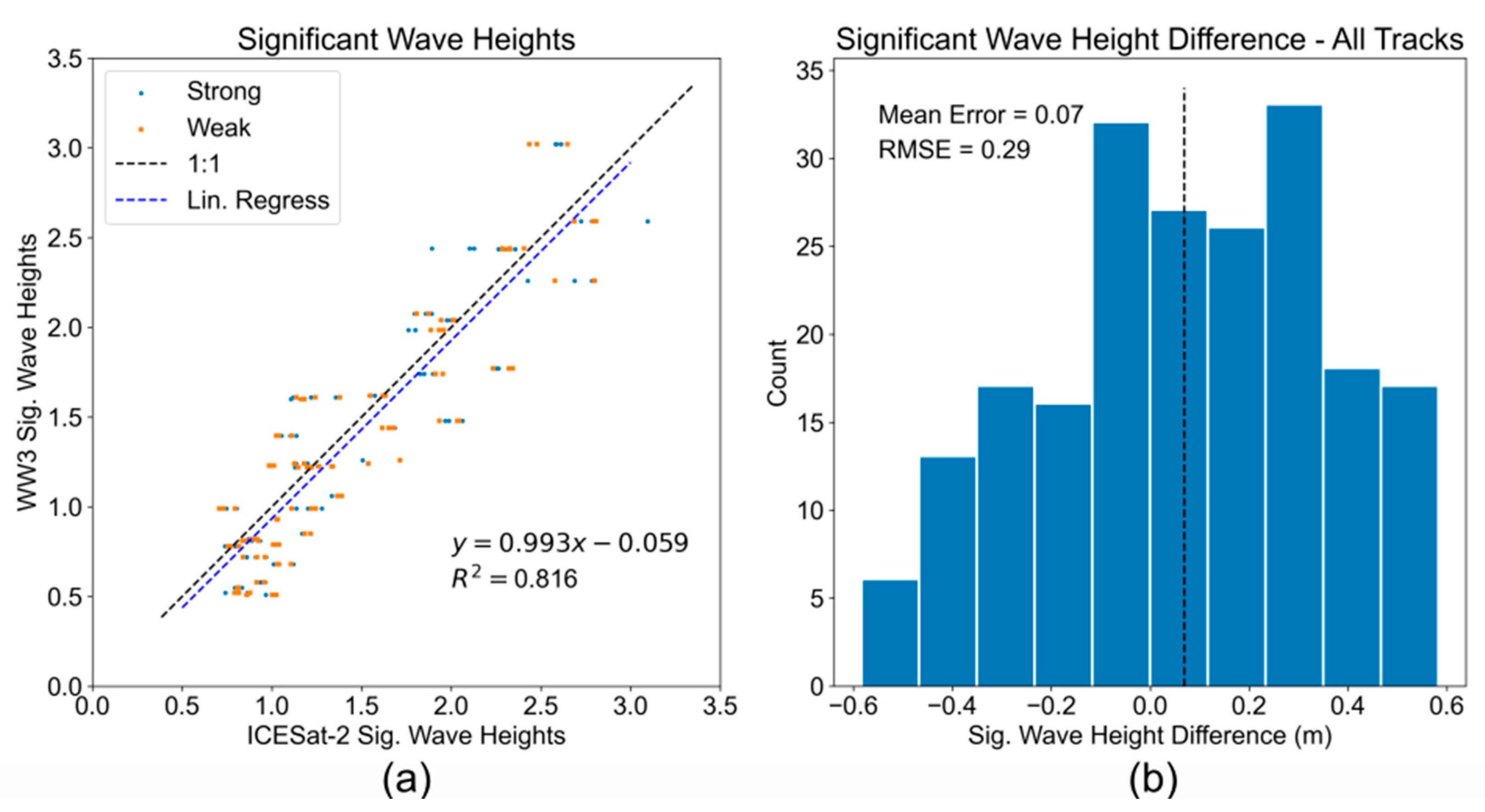
3.1. Wave Height
3.2. Wavelength
3.3. Wavelets
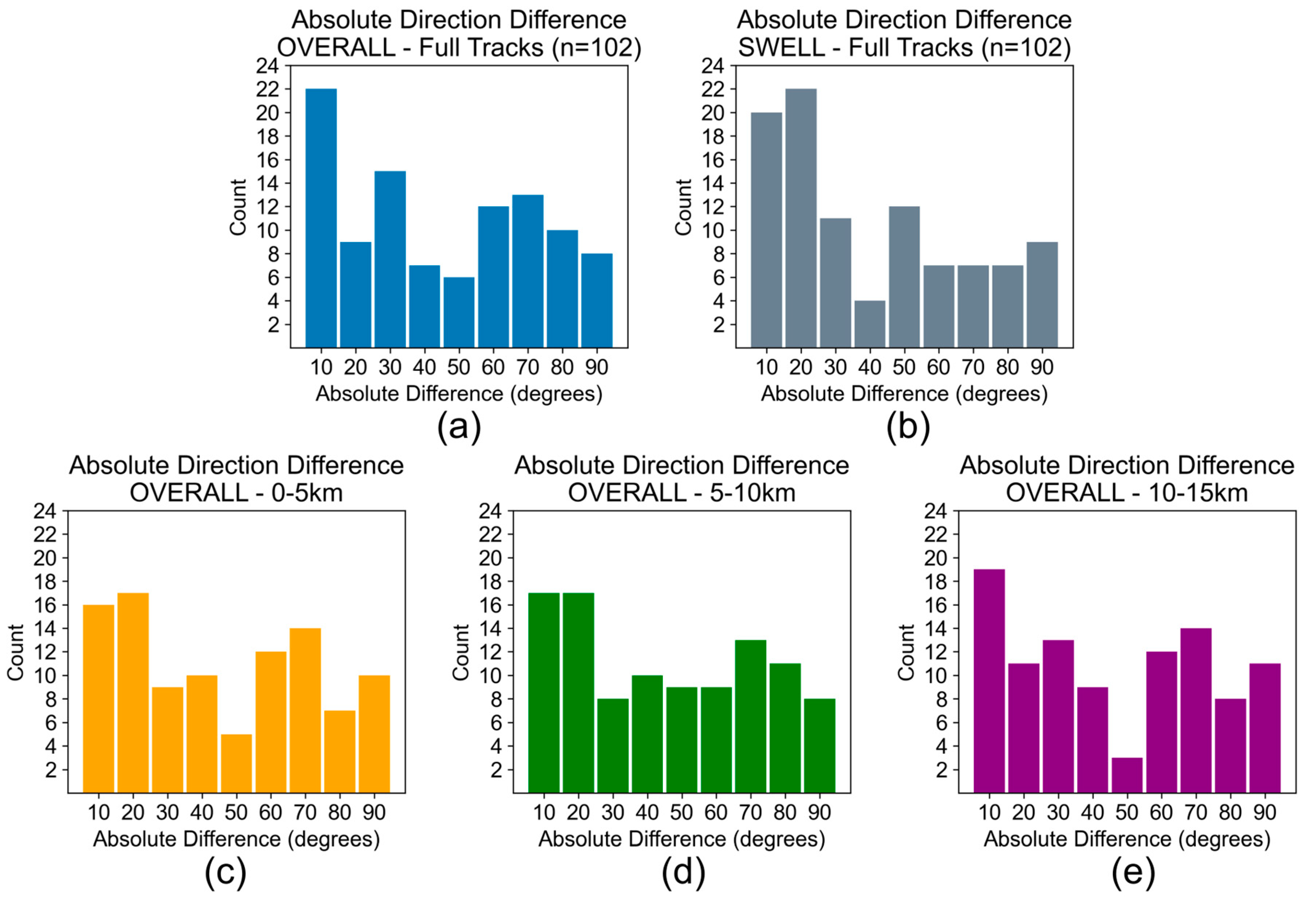
3.4. Directionality
4. Discussion
4.1. Basic Wave Metrics
4.2. Wavelets
4.3. Directionality
5. Conclusions
Author Contributions
Funding
Data Availability Statement
Acknowledgments
Conflicts of Interest
Appendix A

| O’ahu | Kaua’i | North Carolina | ||||||
|---|---|---|---|---|---|---|---|---|
| Date | RGT | Beams | Date | RGT | Beams | Date | RGT | Beams |
| 5 December 2020 | 1105 | 1, 2, 3 | 17 October 2018 | 282 | 1, 2, 3 | 1 October 2019 | 65 | 1, 2, 3 |
| 4 March 2022 | 1105 | 1, 2, 3 | 15 October 2019 | 282 | 1, 2, 3 | 29 June 2020 | 65 | 1, 2, 3 |
| 2 September 2022 | 1105 | 1, 2, 3 | 11 January 2021 | 282 | 1, 2, 3 | 28 December 2020 | 65 | 1, 2 |
| 15 September 2019 | 1219 | 1 | 12 April 2021 | 282 | 1, 2, 3 | 27 June 2021 | 65 | 1, 2, 3 |
| 13 December 2020 | 1219 | 1, 2, 3 | 9 October 2022 | 282 | 1, 2, 3 | 26 September 2021 | 65 | 1, 2, 3 |
| 12 March 2022 | 1219 | 1, 2, 3 | 20 June 2021 | 1341 | 1, 2, 3 | 26 December 2021 | 65 | 1, 2, 3 |
| 17 September 2022 | 1341 | 1, 2, 3 | 27 March 2022 | 65 | 1, 2, 3 | |||
| 26 June 2022 | 65 | 1, 2, 3 | ||||||
| 24 September 2022 | 65 | 1, 2, 3 | ||||||
| 1 March 2020 | 1010 | 2, 3 | ||||||
| 29 November 2020 | 1010 | 1, 2, 3 | ||||||
| 28 February 2021 | 1010 | 1, 2, 3 | ||||||
| 27 November 2021 | 1010 | 1, 2, 3 | ||||||
| 27 December 2018 | 1368 | 1, 2, 3 | ||||||
| 28 March 2019 | 1368 | 1, 2, 3 | ||||||
| 25 September 2019 | 1368 | 1, 2, 3 | ||||||
| 25 December 2019 | 1368 | 1, 2, 3 | ||||||
| 24 June 2020 | 1368 | 1, 2, 3 | ||||||
| 22 September 2020 | 1368 | 1, 2, 3 | ||||||
| 22 December 2020 | 1368 | 1, 2, 3 | ||||||
| 22 June 2021 | 1368 | 1, 2, 3 | ||||||
| 21 March 2022 | 1368 | 1, 2, 3 | ||||||
| 19 September 2022 | 1368 | 1, 2, 3 |
References
- Hauer, M.E.; Fussell, E.; Mueller, V.; Burkett, M.; Call, M.; Abel, K.; McLeman, R.; Wrathall, D. Sea-Level Rise and Human Migration. Nat. Rev. Earth Env. 2020, 1, 28–39. [Google Scholar] [CrossRef]
- Toimil, A.; Losada, I.J.; Nicholls, R.J.; Dalrymple, R.A.; Stive, M.J.F. Addressing the Challenges of Climate Change Risks and Adaptation in Coastal Areas: A Review. Coast. Eng. 2020, 156, 103611. [Google Scholar] [CrossRef]
- Vandeweerd, V.; Bernal, P.; Belfiore, S.; Goldstein, K.; Cicin-Sain, B. A Guide to Oceans, Coasts, and Islands at the World Summit on Sustainable Development; Center for the Study of Marine Policy: Woods Hole, MA, USA, 2002. [Google Scholar]
- Manes, S.; Gama-Maia, D.; Vaz, S.; Pires, A.P.F.; Tardin, R.H.; Maricato, G.; Bezerra, D.D.S.; Vale, M.M. Nature as a Solution for Shoreline Protection against Coastal Risks Associated with Ongoing Sea-Level Rise. Ocean Coast. Manag. 2023, 235, 106487. [Google Scholar] [CrossRef]
- Vousdoukas, M.I.; Mentaschi, L.; Voukouvalas, E.; Verlaan, M.; Jevrejeva, S.; Jackson, L.P.; Feyen, L. Global Probabilistic Projections of Extreme Sea Levels Show Intensification of Coastal Flood Hazard. Nat. Commun. 2018, 9, 2360. [Google Scholar] [CrossRef] [PubMed]
- Ardhuin, F.; Stopa, J.E.; Chapron, B.; Collard, F.; Husson, R.; Jensen, R.E.; Johannessen, J.; Mouche, A.; Passaro, M.; Quartly, G.D.; et al. Observing Sea States. Front. Mar. Sci. 2019, 6, 124. [Google Scholar] [CrossRef]
- Centurioni, L.; Braasch, L.; Lauro, E.D.; Contestabile, P.; Leo, F.D.; Casotti, R.; Franco, L.; Vicinanza, D. A new strategic wave measurement station off naples port main breakwater. Coast. Eng. Proc. 2016, 1, 36. [Google Scholar] [CrossRef]
- Li, M.; Zhang, S.; Qi, Z.; Dang, C. Application of Wave Drifter to Marine Environment Observation. In Proceedings of the OCEANS 2016, Shanghai, China, 10–13 April 2016; pp. 1–5. [Google Scholar]
- Lumpkin, R.; Özgökmen, T.; Centurioni, L. Advances in the Application of Surface Drifters. Annu. Rev. Mar. Sci. 2017, 9, 59–81. [Google Scholar] [CrossRef]
- Pearman, D.W.; Herbers, T.H.C.; Janssen, T.T.; van Ettinger, H.D.; McIntyre, S.A.; Jessen, P.F. Drifter Observations of the Effects of Shoals and Tidal-Currents on Wave Evolution in San Francisco Bight. Cont. Shelf Res. 2014, 91, 109–119. [Google Scholar] [CrossRef]
- Figa-Saldaña, J.; Wilson, J.J.W.; Attema, E.; Gelsthorpe, R.; Drinkwater, M.R.; Stoffelen, A. The Advanced Scatterometer (ASCAT) on the Meteorological Operational (MetOp) Platform: A Follow on for European Wind Scatterometers. Can. J. Remote Sens. 2002, 28, 404–412. [Google Scholar] [CrossRef]
- Wang, H.; Mouche, A.; Husson, R.; Chapron, B.; Yang, J.; Liu, J.; Ren, L. Quantifying Uncertainties in the Partitioned Swell Heights Observed From CFOSAT SWIM and Sentinel-1 SAR via Triple Collocation. IEEE Trans. Geosci. Remote Sens. 2022, 60, 4207716. [Google Scholar] [CrossRef]
- Hauser, D.; Abdalla, S.; Ardhuin, F.; Bidlot, J.-R.; Bourassa, M.; Cotton, D.; Gommenginger, C.; Evers-King, H.; Johnsen, H.; Knaff, J.; et al. Satellite Remote Sensing of Surface Winds, Waves, and Currents: Where Are We Now? Surv. Geophys. 2023, 44, 1357–1446. [Google Scholar] [CrossRef]
- Villas Bôas, A.B.; Ardhuin, F.; Ayet, A.; Bourassa, M.A.; Brandt, P.; Chapron, B.; Cornuelle, B.D.; Farrar, J.T.; Fewings, M.R.; Fox-Kemper, B.; et al. Integrated Observations of Global Surface Winds, Currents, and Waves: Requirements and Challenges for the Next Decade. Front. Mar. Sci. 2019, 6, 425. [Google Scholar] [CrossRef]
- Huang, L.; Fan, C.; Meng, J.; Yang, J.; Zhang, J. Shallow Sea Topography Detection Using Fully Polarimetric Gaofen-3 SAR Data Based on Swell Patterns. Acta Oceanol. Sin. 2023, 42, 150–162. [Google Scholar] [CrossRef]
- Zamparelli, V.; De Santi, F.; De Carolis, G.; Fornaro, G. SAR Based Sea Surface Complex Wind Fields Estimation: An Analysis over the Northern Adriatic Sea. Remote Sens. 2023, 15, 2074. [Google Scholar] [CrossRef]
- Brunt, K.M.; Neumann, T.A.; Smith, B.E. Assessment of ICESat-2 Ice Sheet Surface Heights, Based on Comparisons Over the Interior of the Antarctic Ice Sheet. Geophys. Res. Lett. 2019, 46, 13072–13078. [Google Scholar] [CrossRef]
- Brunt, K.M.; Neumann, T.A.; Larsen, C.F. Assessment of Altimetry Using Ground-Based GPS Data from the 88S Traverse, Antarctica, in Support of ICESat-2. Cryosphere 2019, 13, 579–590. [Google Scholar] [CrossRef]
- Klotz, B.W.; Neuenschwander, A.; Magruder, L.A. High-Resolution Ocean Wave and Wind Characteristics Determined by the ICESat-2 Land Surface Algorithm. Geophys. Res. Lett. 2020, 47, e2019GL085907. [Google Scholar] [CrossRef]
- Yu, Y.; Sandwell, D.T.; Gille, S.T.; Villas Bôas, A.B. Assessment of ICESat-2 for the Recovery of Ocean Topography. Geophys. J. Int. 2021, 226, 456–467. [Google Scholar] [CrossRef]
- Horvat, C.; Blanchard-Wrigglesworth, E.; Petty, A. Observing Waves in Sea Ice With ICESat-2. Geophys. Res. Lett. 2020, 47, e2020GL087629. [Google Scholar] [CrossRef]
- Nilsson, B.; Andersen, O.B.; Ranndal, H.; Rasmussen, M.L. Consolidating ICESat-2 Ocean Wave Characteristics with CryoSat-2 during the CRYO2ICE Campaign. Remote Sens. 2022, 14, 1300. [Google Scholar] [CrossRef]
- Cao, B.; Fang, Y.; Gao, L.; Hu, H.; Jiang, Z.; Sun, B.; Lou, L. An Active-Passive Fusion Strategy and Accuracy Evaluation for Shallow Water Bathymetry Based on ICESat-2 ATLAS Laser Point Cloud and Satellite Remote Sensing Imagery. Int. J. Remote Sens. 2021, 42, 2783–2806. [Google Scholar] [CrossRef]
- Chen, Y.; Chen, Y.; Zhu, Z.; Le, Y.; Qiu, Z.; Chen, G.; Wang, L.; Wang, L. Refraction Correction and Coordinate Displacement Compensation in Nearshore Bathymetry Using ICESat-2 Lidar Data and Remote-Sensing Images. Opt. Express OE 2021, 29, 2411–2430. [Google Scholar] [CrossRef] [PubMed]
- Leng, Z.; Zhang, J.; Ma, Y.; Zhang, J.; Zhu, H. A Novel Bathymetry Signal Photon Extraction Algorithm for Photon-Counting LiDAR Based on Adaptive Elliptical Neighborhood. Int. J. Appl. Earth Obs. Geoinf. 2022, 115, 103080. [Google Scholar] [CrossRef]
- Parrish, C.E.; Magruder, L.A.; Neuenschwander, A.L.; Forfinski-Sarkozi, N.; Alonzo, M.; Jasinski, M. Validation of ICESat-2 ATLAS Bathymetry and Analysis of ATLAS’s Bathymetric Mapping Performance. Remote Sens. 2019, 11, 1634. [Google Scholar] [CrossRef]
- Ranndal, H.; Sigaard Christiansen, P.; Kliving, P.; Baltazar Andersen, O.; Nielsen, K. Evaluation of a Statistical Approach for Extracting Shallow Water Bathymetry Signals from ICESat-2 ATL03 Photon Data. Remote Sens. 2021, 13, 3548. [Google Scholar] [CrossRef]
- Yang, J.; Ma, Y.; Zheng, H.; Xu, N.; Zhu, K.; Wang, X.H.; Li, S. Derived Depths in Opaque Waters Using ICESat-2 Photon-Counting Lidar. Geophys. Res. Lett. 2022, 49, e2022GL100509. [Google Scholar] [CrossRef]
- Bernardis, M.; Nardini, R.; Apicella, L.; Demarte, M.; Guideri, M.; Federici, B.; Quarati, A.; De Martino, M. Use of ICEsat-2 and Sentinel-2 Open Data for the Derivation of Bathymetry in Shallow Waters: Case Studies in Sardinia and in the Venice Lagoon. Remote Sens. 2023, 15, 2944. [Google Scholar] [CrossRef]
- Yang, J.; Ma, Y.; Zheng, H.; Gu, Y.; Zhou, H.; Li, S. Analysis and Correction of Water Forward-Scattering-Induced Bathymetric Bias for Spaceborne Photon-Counting Lidar. Remote Sens. 2023, 15, 931. [Google Scholar] [CrossRef]
- Stumpf, R.P.; Holderied, K.; Sinclair, M. Determination of Water Depth with High-Resolution Satellite Imagery over Variable Bottom Types. Limnol. Oceanogr. 2003, 48, 547–556. [Google Scholar] [CrossRef]
- Albright, A.; Glennie, C. Nearshore Bathymetry From Fusion of Sentinel-2 and ICESat-2 Observations. IEEE Geosci. Remote Sens. Lett. 2021, 18, 900–904. [Google Scholar] [CrossRef]
- Babbel, B.J.; Parrish, C.E.; Magruder, L.A. ICESat-2 Elevation Retrievals in Support of Satellite-Derived Bathymetry for Global Science Applications. Geophys. Res. Lett. 2021, 48, e2020GL090629. [Google Scholar] [CrossRef] [PubMed]
- Ma, Y.; Xu, N.; Liu, Z.; Yang, B.; Yang, F.; Wang, X.H.; Li, S. Satellite-Derived Bathymetry Using the ICESat-2 Lidar and Sentinel-2 Imagery Datasets. Remote Sens. Environ. 2020, 250, 112047. [Google Scholar] [CrossRef]
- Thomas, N.; Lee, B.; Coutts, O.; Bunting, P.; Lagomasino, D.; Fatoyinbo, L. A Purely Spaceborne Open Source Approach for Regional Bathymetry Mapping. IEEE Trans. Geosci. Remote Sens. 2022, 60, 4708109. [Google Scholar] [CrossRef]
- Daly, C.; Baba, W.; Bergsma, E.; Thoumyre, G.; Almar, R.; Garlan, T. The New Era of Regional Coastal Bathymetry from Space: A Showcase for West Africa Using Optical Sentinel-2 Imagery. Remote Sens. Environ. 2022, 278, 113084. [Google Scholar] [CrossRef]
- Scripps Institution of Oceanography Coastal Data Information Program Buoy Data. Available online: https://cdip.ucsd.edu/ (accessed on 12 May 2023).
- Magruder, L.; Brunt, K.; Neumann, T.; Klotz, B.; Alonzo, M. Passive Ground-Based Optical Techniques for Monitoring the On-Orbit ICESat-2 Altimeter Geolocation and Footprint Diameter. Earth Space Sci. 2021, 8, e2020EA001414. [Google Scholar] [CrossRef]
- Markus, T.; Neumann, T.; Martino, A.; Abdalati, W.; Brunt, K.; Csatho, B.; Farrell, S.; Fricker, H.; Gardner, A.; Harding, D.; et al. The Ice, Cloud, and Land Elevation Satellite-2 (ICESat-2): Science Requirements, Concept, and Implementation. Remote Sens. Environ. 2017, 190, 260–273. [Google Scholar] [CrossRef]
- Martino, A.J.; Neumann, T.A.; Kurtz, N.T.; McLennan, D. ICESat-2 Mission Overview and Early Performance. In Proceedings of the Sensors, Systems, and Next-Generation Satellites XXIII, SPIE, Strasbourg, France, 9–12 September 2019; Volume 11151, pp. 68–77. [Google Scholar]
- Schutz, B.E.; Zwally, H.J.; Shuman, C.A.; Hancock, D.; DiMarzio, J.P. Overview of the ICESat Mission. Geophys. Res. Lett. 2005, 32, L21S01. [Google Scholar] [CrossRef]
- Neumann, T.A.; Martino, A.J.; Markus, T.; Bae, S.; Bock, M.R.; Brenner, A.C.; Brunt, K.M.; Cavanaugh, J.; Fernandes, S.T.; Hancock, D.W.; et al. The Ice, Cloud, and Land Elevation Satellite—2 Mission: A Global Geolocated Photon Product Derived from the Advanced Topographic Laser Altimeter System. Remote Sens. Environ. 2019, 233, 111325. [Google Scholar] [CrossRef]
- Luthcke, S.B.; Thomas, T.C.; Pennington, T.A.; Rebold, T.W.; Nicholas, J.B.; Rowlands, D.D.; Gardner, A.S.; Bae, S. ICESat-2 Pointing Calibration and Geolocation Performance. Earth Space Sci. 2021, 8, e2020EA001494. [Google Scholar] [CrossRef]
- Neumann, T.A.; Brenner, A.; Hancock, D.; Robbins, J.; Saba, J.; Harbeck, K.; Gibbons, A.; Lee, J.; Luthcke, S.B.; Rebold, T. ATLAS/ICESat-2 L2A Global Geolocated Photon Data, Version 5. 2021. Available online: https://nsidc.org/data/atl03/versions/5 (accessed on 24 May 2023).
- Morison, J.H.; Hancock, D.; Dickinson, S.; Robbins, J.; Roberts, L.; Kwok, R.; Palm, S.P.; Smith, B.; Jasinski, M.F. ICESat-2 Science Team ATLAS/ICESat-2 L3A Ocean Surface Height, Version 5. 2022. Available online: https://nsidc.org/data/atl12/versions/5 (accessed on 1 June 2023).
- Jasinski, M.F.; Stoll, J.D.; Hancock, D.; Robbins, J.; Nattala, J.; Morison, J.; Jones, B.M.; Ondrusek, M.E.; Pavelsky, T.M.; Parrish, C.; et al. ATLAS/ICESat-2 L3A Along Track Inland Surface Water Data, Version 5. 2021. Available online: https://nsidc.org/data/atl13/versions/5 (accessed on 1 June 2023).
- Cheung, K.F. WaveWatch III (WW3) Global Wave Model 2023. Available online: https://catalog.data.gov/dataset/wavewatch-iii-ww3-global-wave-model (accessed on 30 May 2023).
- Tolman, H.L. Testing of WAVEWATCH III Version 2.22 in NCEP’s NWW3 Ocean Wave Model Suite; NOAA/NWS/NCEP/OMB Technical Note; NOAA National Centers for Environmental Prediction: Washington, DC, USA, 2002; p. 99.
- NOAA National Centers for Environmental Prediction GFS-Wave Buoy Verification. Available online: https://polar.ncep.noaa.gov/waves/validation/gfsv16/buoys/? (accessed on 21 September 2023).
- Stewart, R.H. Introduction to Physical Oceanography. 2008. Available online: https://www.uv.es/hegigui/Kasper/por%20Robert%20H%20Stewart.pdf (accessed on 5 May 2023).
- Lomb, N.R. Least-Squares Frequency Analysis of Unequally Spaced Data. Astrophys. Space Sci. 1976, 39, 447–462. [Google Scholar] [CrossRef]
- Scargle, J.D. Studies in Astronomical Time Series Analysis. II. Statistical Aspects of Spectral Analysis of Unevenly Spaced Data. Astrophys. J. 1982, 263, 835–853. [Google Scholar] [CrossRef]
- VanderPlas, J.T. Understanding the Lomb–Scargle Periodogram. ApJS 2018, 236, 16. [Google Scholar] [CrossRef]
- The Astropy Collaboration; Price-Whelan, A.M.; Lim, P.L.; Earl, N.; Starkman, N.; Bradley, L.; Shupe, D.L.; Patil, A.A.; Corrales, L.; Brasseur, C.E.; et al. The Astropy Project: Sustaining and Growing a Community-Oriented Open-Source Project and the Latest Major Release (v5.0) of the Core Package. ApJ 2022, 935, 167. [Google Scholar] [CrossRef]
- Drennan, W.M.; Graber, H.C.; Hauser, D.; Quentin, C. On the Wave Age Dependence of Wind Stress over Pure Wind Seas. J. Geophys. Res. Ocean. 2003, 108, 8062. [Google Scholar] [CrossRef]
- Drennan, W.M.; Taylor, P.K.; Yelland, M.J. Parameterizing the Sea Surface Roughness. J. Phys. Oceanogr. 2005, 35, 835–848. [Google Scholar] [CrossRef]
- Taylor, P.K.; Yelland, M.J. The Dependence of Sea Surface Roughness on the Height and Steepness of the Waves. J. Phys. Oceanogr. 2001, 31, 572–590. [Google Scholar] [CrossRef]
- Foster, G. Wavelets for Period Analysis of Unevenly Sampled Time Series. Astron. J. 1996, 112, 1709. [Google Scholar] [CrossRef]
- Dorn-Wallenstein, T.; Desai, A.; Gilbert, G.; RT, A.; Monsue, T. JazzHands 2020.
- Virtanen, P.; Gommers, R.; Oliphant, T.E.; Haberland, M.; Reddy, T.; Cournapeau, D.; Burovski, E.; Peterson, P.; Weckesser, W.; Bright, J.; et al. SciPy 1.0: Fundamental Algorithms for Scientific Computing in Python. Nat. Methods 2020, 17, 261–272. [Google Scholar] [CrossRef]
- Khan, S.S.; Echevarria, E.R.; Hemer, M.A. Ocean Swell Comparisons Between Sentinel-1 and WAVEWATCH III Around Australia. J. Geophys. Res. Ocean. 2021, 126, e2020JC016265. [Google Scholar] [CrossRef]
- Wang, H.; Mouche, A.; Husson, R.; Grouazel, A.; Chapron, B.; Yang, J. Assessment of Ocean Swell Height Observations from Sentinel-1A/B Wave Mode against Buoy In Situ and Modeling Hindcasts. Remote Sens. 2022, 14, 862. [Google Scholar] [CrossRef]
- Santos, D.; Abreu, T.; Silva, P.A.; Baptista, P. Estimation of Coastal Bathymetry Using Wavelets. J. Mar. Sci. Eng. 2020, 8, 772. [Google Scholar] [CrossRef]
- Santos, D.; Fernández-Fernández, S.; Abreu, T.; Silva, P.A.; Baptista, P. Retrieval of Nearshore Bathymetry from Sentinel-1 SAR Data in High Energetic Wave Coasts: The Portuguese Case Study. Remote Sens. Appl. Soc. Environ. 2022, 25, 100674. [Google Scholar] [CrossRef]
- Almar, R.; Bergsma, E.W.J.; Thoumyre, G.; Baba, M.W.; Cesbron, G.; Daly, C.; Garlan, T.; Lifermann, A. Global Satellite-Based Coastal Bathymetry from Waves. Remote Sens. 2021, 13, 4628. [Google Scholar] [CrossRef]
- Neuenschwander, A.; Magruder, L.; Guenther, E.; Hancock, S.; Purslow, M. Radiometric Assessment of ICESat-2 over Vegetated Surfaces. Remote Sens. 2022, 14, 787. [Google Scholar] [CrossRef]


| Dataset | Source | Data Type | Resolution | Parameters |
|---|---|---|---|---|
| ATL03 | NSIDC | Photon Return Point Cloud | ~0.7 m along track | Photon Location (x, y, z) Derived classifications |
| WW3 | PacIOOS | Raster | 0.5° × 0.5° | Peak wave direction Peak wave period Significant wave height:
|
| Compass Angle | Apparent Wavelength Factor | Theoretical Lag/Offset Distance for Directionality (m) |
|---|---|---|
| 0/180° | 100.1% | 3.1428 |
| 15/195° | 104.6% | 27.5009 |
| 30/210° | 117.9% | 56.2059 |
| 45/225° | 146.6% | 96.4563 |
| 60/240° | 213.0% | 169.1642 |
| 75/255° | 444.5% | 389.5973 |
| 86–90/266–270° | 2865%–∞ | 2577–∞ |
| 105/285° | 342.0% | −294.195 |
| 120/300° | 188.7% | −143.94 |
| 135/315° | 136.7% | −83.8733 |
| 150/330° | 113.3% | −47.8228 |
| 165/345° | 102.6% | −20.7636 |
Disclaimer/Publisher’s Note: The statements, opinions and data contained in all publications are solely those of the individual author(s) and contributor(s) and not of MDPI and/or the editor(s). MDPI and/or the editor(s) disclaim responsibility for any injury to people or property resulting from any ideas, methods, instructions or products referred to in the content. |
© 2023 by the authors. Licensee MDPI, Basel, Switzerland. This article is an open access article distributed under the terms and conditions of the Creative Commons Attribution (CC BY) license (https://creativecommons.org/licenses/by/4.0/).
Share and Cite
Dietrich, J.T.; Magruder, L.A.; Holwill, M. Monitoring Coastal Waves with ICESat-2. J. Mar. Sci. Eng. 2023, 11, 2082. https://doi.org/10.3390/jmse11112082
Dietrich JT, Magruder LA, Holwill M. Monitoring Coastal Waves with ICESat-2. Journal of Marine Science and Engineering. 2023; 11(11):2082. https://doi.org/10.3390/jmse11112082
Chicago/Turabian StyleDietrich, James T., Lori A. Magruder, and Matthew Holwill. 2023. "Monitoring Coastal Waves with ICESat-2" Journal of Marine Science and Engineering 11, no. 11: 2082. https://doi.org/10.3390/jmse11112082
APA StyleDietrich, J. T., Magruder, L. A., & Holwill, M. (2023). Monitoring Coastal Waves with ICESat-2. Journal of Marine Science and Engineering, 11(11), 2082. https://doi.org/10.3390/jmse11112082