The Contact Angle Hysteresis Puzzle

Abstract

This short review explains the essence of the theory of contact angle hysteresis. It emphasizes the controversial points and discusses the shortcomings of contact angle hysteresis measurements. The review ends with conclusions regarding the improvements that are required to make these measurements useful for the characterization of surface wettability.

1. Introduction

It has been known for over 200 years that when a liquid body meets a solid surface, an angle is formed between the tangents to the solid and the liquid at the points of contact [1]. This angle (measured on the liquid side) is called the “contact angle” (CA) and is shown in Figure 1a. The dependence of this CA on the surface properties of the solid and the liquid is supposed to be summarized by the Young equation that reads [1]

$$cos{\theta }_Y=\frac{{\sigma }_s-{\sigma }_{sl}}{{\sigma }_{lf}}$$

(1)

where ${\theta }_Y$ is the Young CA, $\sigma$ is surface or interfacial tension and the subscripts s, l, and f represent the solid, liquid, and fluid, respectively.

However, while the Young equation considers only surface tensions, measured CAs are known to depend also on other properties of the solid surface, such as roughness or chemical heterogeneity. Therefore, the Young equation is valid only for surfaces that are homogeneous, smooth, rigid, isotropic, insoluble in the liquid and fluid, and not reactive with them. Such a solid surface is called “ideal.” At this point, it is important to distinguish between two types of CAs. The actual CA is the local, microscopic CA, which is not yet accessible to experimental measurement. It was shown by a few independent theoretical studies [2,3,4] that the actual CA is the one that is described by the Young equation. On the other hand, the apparent CA is the experimentally measured CA. On an ideal solid surface, the actual and apparent CAs are identical, but on a rough surface, for example, they may be very different (please see Figure 1b). So, as was realized long ago, the ideal picture of a single CA that characterizes the wettability of a solid surface, does not apply to real solid surfaces. In real systems, there exists a range of apparent CAs that is called “CA hysteresis” (CAH) [5]. The highest and lowest apparent CAs are called “advancing” and “receding”, respectively.

The phenomenon of hysteresis is an important player in the wettability assessment of solid surfaces [6]. The mere existence of CAH makes it impossible to exactly define a unique, characteristic CA. Moreover, different experimental setups may lead to different values for the advancing and receding angles. Thus, there is a need to solve this problem and standardize the measurement of CAs. The most common way to measure the advancing CA is to put a drop on a surface, and gradually increase the volume of the drop until it starts to spontaneously spread. The CA at this point is the advancing one. The same procedure in the opposite direction leads to the receding CA. Below we will discuss this point further. However, it is not known yet whether this is the most meaningful way to define the hysteresis range. A different way, for example, is to use a tilted surface, and measure the CA at the front and at the back of the drop [7]. However, it was demonstrated [8] that these CAs cannot be simultaneously equal to those measured with a symmetric drop that sits on a horizontal surface. Thus, it is not yet clear which method is more useful.

In addition to the role of CAH in the characterization of solid surfaces, it has implications in other fields, such as biology and industry. A famous example in biology is the “Lotus effect” [9] that implies the non-wettability of the solid surface. Drops that collide with such a surface easily roll off, an action that depends on CAH being minimal. In industry, for example, the oil and gas industry [10], the involved surfaces are usually rough and chemically heterogeneous. CAH must have a major role in the analysis of such systems, but this effect is not always considered.

The concept of hysteresis is a general one [11] and is relevant to many scientific disciplines. Hysteresis implies system behavior that depends on the history of the system. From a thermodynamic point of view, history dependence occurs when there are multiple equilibrium states of the system [11,12]. Obviously, only one of them that has the lowest Gibbs energy is stable. To emphasize this point, it is called the “most stable CA” [6]. All the other equilibrium states are metastable. It is possible for the system to move from one metastable state to another of lower energy if it has enough energy to overcome the energy barrier that evidently exists between each pair of metastable equilibrium states. An important point to realize is that the metastable states are still equilibrium states; therefore, they may be modeled by thermodynamic methods. At this point, it is worthwhile to make a comment about terminology: It is better to avoid using the term “dynamic CA” that was introduced into the literature many years ago to describe CAs within the hysteresis range. This term may be misleading, because the CAs that are measured are associated with metastable equilibrium states. The term “dynamic CA” should be reserved for the phenomenon of the dependence of the CA on the speed of motion of the contact line.

The present short review attempts to focus on the discrepancy between our reasonable understanding of the physics of CAH, and the practical difficulties involved in CAH measurement and interpretation. More general reviews that describe a few models of CAH exist in the literature, e.g., [13,14,15]. This paper focuses on the approach of Johnson and Dettre [5] and its extension by the author, because it seems to be the simplest, most straightforward approach. It explains the physical background using a very simple model; then, the shortcomings of CAH measurement are discussed.

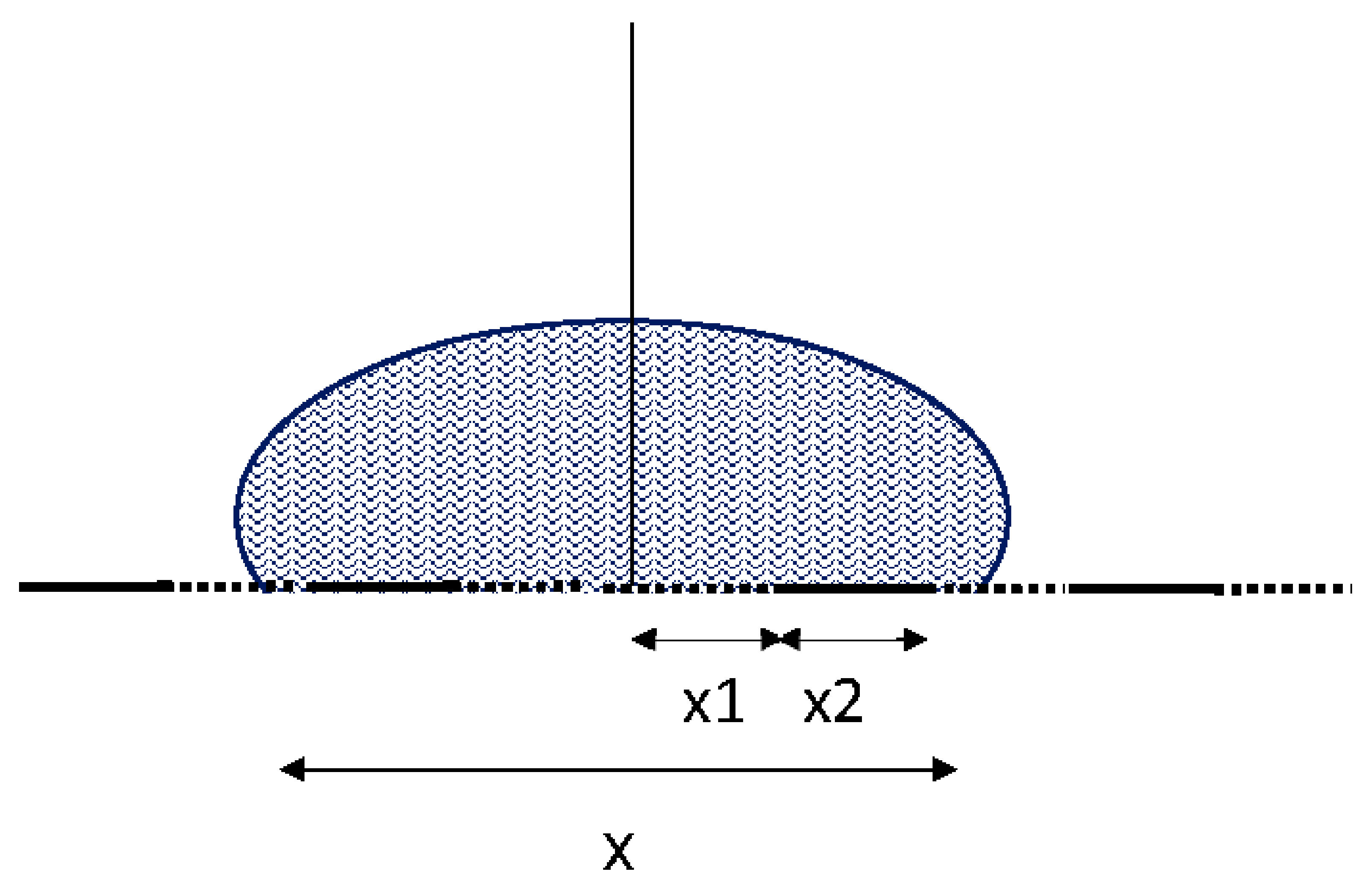
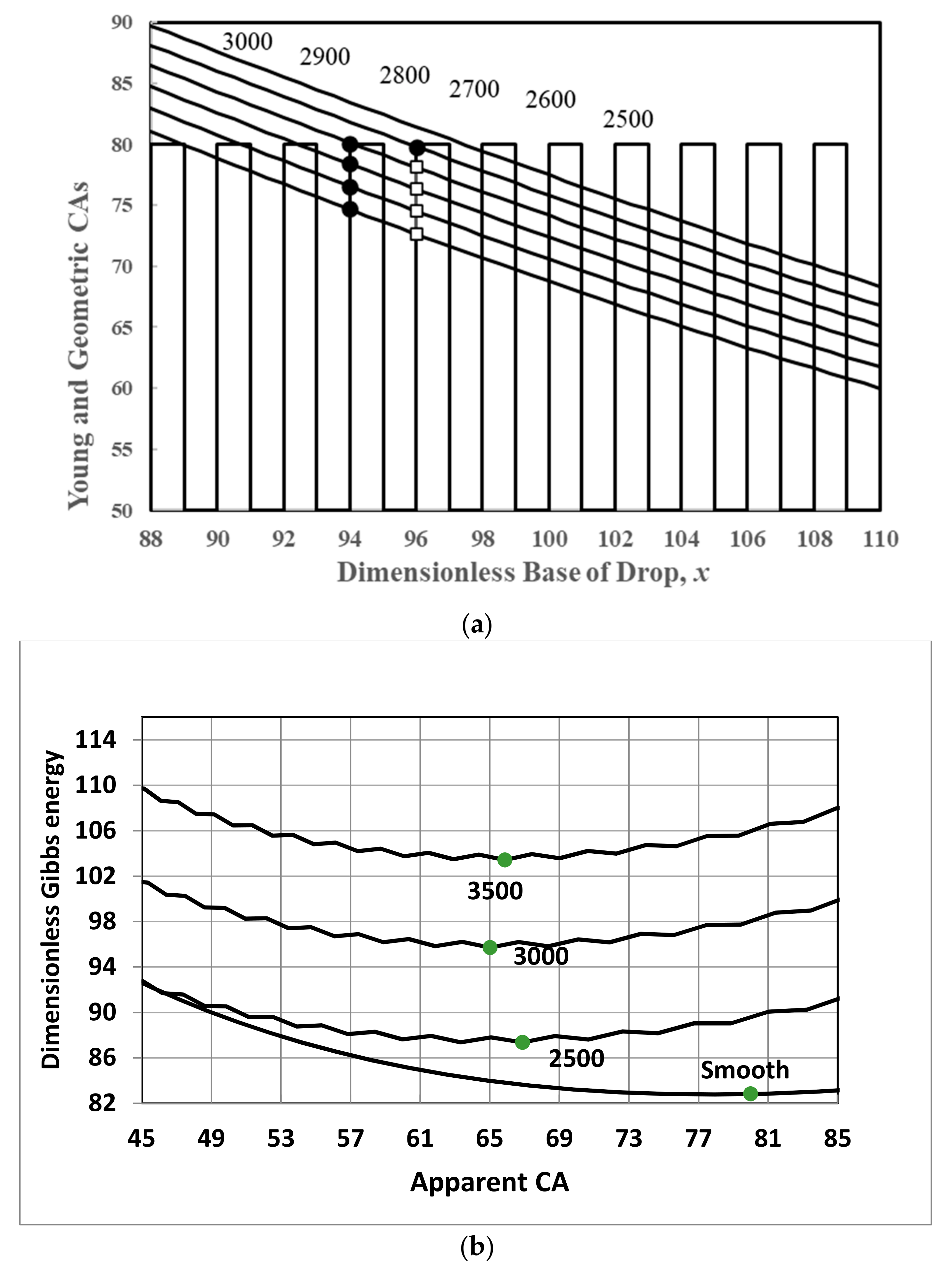
2. A Very Simple Model of a Real Surface

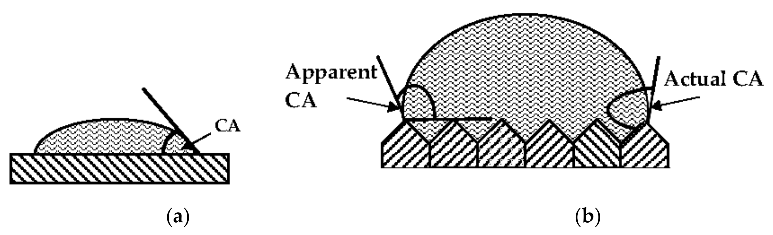
The pioneering work on models of CAH was carried out by Johnson and Dettre [5]. Perhaps the simplest model that can be imagined based on their approach consists of a two-dimensional, smooth, but chemically heterogeneous solid surface on which a cylindrical drop sits. Figure 2 shows the system for a solid surface made of parallel stripes having alternated Young CAs of θ₁ and θ₂. The drop sits symmetrically on the surface, so each of the contact lines sits on a strip having the same CA. In the absence of gravity, which affects the shape of the drop, but not its CAs, the dimensionless Gibbs energy of the system per unit depth is given by

$$\frac{G}{\sigma }=\frac{\theta x}{sin\theta }-x_{1}cos{\theta }_1-x_{2}cos{\theta }_2$$

(2)

where σ is the surface tension of the liquid, x is the length of the base of the drop, and θ is the apparent CA of the drop. If x_1i is the length of a stripe number i of CA = ${\theta }_1$ that is in touch with the liquid, and similarly, x_2i can be defined for the stripes of CA = ${\theta }_2,$ then $x_1={\displaystyle \sum }_1^{n1}{x}_{1i}$, and $x_2={\displaystyle \sum }_1^{n2}{x}_{2i}.$ n₁ and n₂ are the numbers of stripes characterized by CAs ${\theta }_1$ and ${\theta }_2$, respectively, that are in touch with the liquid (please note that n is not necessarily a whole number because the contact lines of the drop do not always sit on the border between stripes, although in practice this is usually the case). The first term on the right-hand side of Equation (2) stands for the dimensionless energy per unit depth that is associated with the length of the arc that the liquid cross section makes with the air, and the other two terms give the dimensionless energy per unit depth that is associated with the length of contact between the solid and the liquid. If the contact lines are on surface 1, the actual CA must be θ₁. When they are on surface 2, the actual CA is θ₂. When they are on the line in-between surface 1 and surface 2, the CA may have any value between θ₁ and θ₂, depending on the geometry of the drop. The dimensionless “volume” per unit depth (dimensionless cross-section area, A) of the drop is given by any elementary geometry book as

$$\frac{8A}{x^2}=\frac{2{\theta }_g-\mathit{sin}\left(2{\theta }_g\right)}{si{n}^2{\theta }_g}$$

(3)

where θ_g is the geometric CA, calculated from the volume of the drop per unit depth, A, and its basis, x. The calculations are carried out for each volume separately, holding it constant for each case.

3. The Cause of CAH

Figure 3a shows two types of curves: one presents the Young CA (the thermodynamic condition) as a periodic step function of position along the two-dimensional surface that jumps in this example between θ₁ = 50° and θ₂ = 80°; the other is a smooth function that shows the geometric CA that corresponds to each base size of the drop for a given volume. The equilibrium state of the drop may exist only if the thermodynamic conditions and the geometric condition yield the same CA, namely, where the two curves intersect. This intersection point is a necessary condition for the existence of a drop in this state; however, it is not a sufficient condition. This is so, because these intersection points represent extremum points that may be maximum or minimum in the Gibbs energy. Obviously, only the minimum points may be stable or metastable. It is important to bring to mind that between two local minima there must be a local maximum. Therefore, between any two intersection points that represent minima in the Gibbs energy, there must be an intersection point that represents a local maximum in the Gibbs energy. The minimum points can be distinguished from the maximum points by identifying the first intersection point of the two curves on the left-hand side of the figure, which must be a minimum point. Thereafter, the intersection points alternate between a minimum and a maximum in the Gibbs energy.

Figure 3b shows the Gibbs energy curves that correspond to the same volume range as in Figure 3a. This figure clearly demonstrates the minima and maxima just described above. The difference in Gibbs energy between a local minimum and the following maximum in the direction of the most stable state is the energy barrier that the drop needs to overcome to get closer to the most stable state.

Figure 3a,b enable the understanding of the basis of CAH [16]. For example, suppose the drop lands on the surface in a state that corresponds to the point marked by a full circle on the curve in Figure 3a for the dimensionless volume of 2500. Now, we increase the volume to 2600, 2700 and 2800. The new intersection points (marked by full circles) show that the position of the contact lines remains the same at the boundary between the two types of stripes, while the CA increases. A small additional increase in volume to 2900 makes the contact lines jump to the next stripe, so that the drop base increases while the CA remains almost the same. Theoretically, this would be defined as the advancing CA. From a macroscopic point of view, it appears as if the contact lines are initially pinned. The present description of the process reveals that initially the contact lines of the drop are not supposed to move, because they are in a metastable state. However, if the surface energy function is a smooth one (for example. sinusoidal [16]), the drop does move, but to a very small extent compared with the changes in the CA, which still looks like pinning.

Figure 3a also enables a simple demonstration of the system’s history dependence. Suppose we start from the last position we reached (dimensionless volume of 2900) and decrease the volume. The contact line remains at the same position, but the CA now decreases. This is a different path (marked by empty squares) than the one that brought the CA to the advancing value by raising the volume. A further reduction in volume brings the contact line to the lowest possible CA that theoretically is defined as the receding CA. Thus, history dependence is the name of the game.

The thermodynamic analysis presented above assumes that there are no external fields involved in determining the equilibrium states of the drop on the surface. Under such an assumption, we define the advancing and receding CAs at the points where the energy barriers are zero. However, in practice, there are always vibrations in the system, because, for example, the building that hosts the laboratory is continually vibrating. Thus, vibrations in the system may mask heterogeneity by making the practical advancing CA smaller than the theoretical value and the receding CA bigger. A detailed analysis of this effect estimates the lowest detectable heterogeneity to be of the order of a few nanometers [17].

4. Effect of CAH on Measurement and Interpretation of CAs

Characterizing the wettability of solid surfaces by its CA is essential for many industrial and biological systems. A critical review of the concept of surface tension of a solid surface has recently been published [18]. So far, ${\sigma }_s$ in the Young equation has been considered as being the wettability characteristic of a solid surface. However, the basic problem is that we do not have a method to measure directly the local, actual CA. Moreover, the procedure of calculating ${\sigma }_s$ from the apparent CA is far from trivial. First, we need to identify the most stable (apparent) CA. This is so, because the equations that enable the calculation of the Young CA from the apparent CA (such as the Wenzel equation) involve the most stable CA (the situation with the Cassie equation is even more complex because there are a few Young CAs).

Nevertheless, we believe that the most stable CA is somewhere between the receding and advancing CAs, as was experimentally demonstrated [19]. Therefore, as a rough approximation, we can assume that the Young CA is some kind of an average of the advancing and receding CAs. Two methods of approximation were suggested in the literature [20]: one is a simple average of the advancing and receding CAs [20], and the other is an average of the cosines of the advancing and receding CAs [21]. Within some range of CAs, the difference between the two averages may be quite small, but it may be as big as about 12%.

The next problem is calculating ${\sigma }_s$ from the estimated value of the Young CA, using Equation (1). This requires a correlation between ${\sigma }_s$ and ${\sigma }_{sl}$. There are quite a few such correlations [22], but all are at least semi-empiric. Thus, the calculation of ${\sigma }_s$ from CAH measurements is still an open problem.

5. Conclusions

• The concepts of advancing and receding CAs are not yet sufficiently well defined, because they depend on the method of measurement as well as on the level of environmental vibrations that cause vibrations of the measuring instrument.
• The main advantage of CAH measurements is their ability to indicate the existence of mechanical or chemical nonuniformity.
• The average of the advancing and receding CAs may serve as a rough approximation for the most stable CA, which enables in some cases (e.g., chemically uniform, rough surfaces) the estimation of the Young CA.
• The above discussed issues call for some standardization of CAH measurement, so consistent results may be universally achieved independently of the laboratory in which they are being measured.

References

1. Young, T. An essay on the cohesion of fluids. Phil. Trans. R. Soc. Lond. 1805, 95, 65–87. [Google Scholar]
2. Neumann, A.W. Wetting, Spreading and Adhesion; Padday, J.F., Ed.; Academic: London, NY, USA, 1978; p. 3. [Google Scholar]
3. Wolansky, G.; Marmur, A. The Actual Contact Angle on a Heterogeneous Rough Surface in Three Dimensions. Langmuir 1998, 14, 5292–5297. [Google Scholar] [CrossRef]
4. Swain, P.S.; Lipowsky, R. Contact angles on heterogeneous surfaces: A new look at Cassie’s and Wenzel’s laws. Langmuir 1998, 14, 6772–6780. [Google Scholar] [CrossRef] [Green Version]
5. Johnson, R.E., Jr.; Dettre, R.H.; Brandreth, M.D. Dynamic contact angle and contact angle hysteresis. J. Colloid Interface Sci. 1977, 62, 205–212. [Google Scholar] [CrossRef]
6. Marmur, A. Solid-Surface Characterization by Wetting. Annu. Rev. Mater. Res. 2009, 39, 473–489. [Google Scholar] [CrossRef]
7. Pierce, E.; Carmona, F.J.; Amirfazli, A. Understanding of sliding and contact angle results in tilted plate experiments. Colloids Surf. A Physicochem. Eng. Asp. 2008, 323, 73–82. [Google Scholar] [CrossRef]
8. Krasovitski, B.; Marmur, A. Drops down the hill: Theoretical study of limiting contact angles and the hysteresis range on a tilted plate. Langmuir 2005, 21, 3881–3885. [Google Scholar] [CrossRef]
9. Neinhuis, C.; Barthlott, W. Characterization and distribution of water-repellent, self-cleaning plant surfaces. Ann. Bot. 1997, 79, 667. [Google Scholar] [CrossRef] [Green Version]
10. Hirasaki, G.J. Wettability: Fundamentals and Surface Forces. SPE Form. Eval. 1991, 6, 217–226. [Google Scholar] [CrossRef]
11. Everett, D.H. A general approach to hysteresis 4. An alternative formulation of the domain model. Trans. Faraday Soc. 1955, 51, 1551–1557. [Google Scholar] [CrossRef]
12. Brandon, S.; Marmur, A. Simulation of Contact Angle Hysteresis on Chemically Heterogeneous Surfaces. J. Colloid Interface Sci. 1996, 183, 351–355. [Google Scholar] [CrossRef] [PubMed]
13. Hans-Jürgen Butt, H.-J.; Liu, J.; Koynov, K.; Straub, B.; Hinduja, C.; Roismann, I.; Berger, R.; Li, X.; Vollmer, D.; Steffen, W.; et al. Contact angle hysteresis. Curr. Opin. Colloid Interface Sci. 2022, 59, 101574. [Google Scholar]
14. Makonen, L. A thermodynamic model of contact angle hysteresis. J. Chem. Phys. 2017, 147, 064703. [Google Scholar] [CrossRef] [PubMed] [Green Version]
15. Eral, H.B.; Mannetje, D.J.C.M.’t.; Oh, J.M. Contact angle hysteresis: A review of fundamentals and applications. Colloid Polym. Sci. 2013, 291, 247–260. [Google Scholar] [CrossRef]
16. Marmur, A. Contact-angle hysteresis on heterogeneous smooth surfaces: Theoretical comparison of the captive bubble and drop methods. Colloids Surf. A Physicochem. Eng. Asp. 1998, 136, 209–215. [Google Scholar] [CrossRef]
17. Bittoun, E.; Marmur, A. Chemical Nano-Heterogeneities Detection by Contact Angle Hysteresis: Theoretical Feasibility. Langmuir 2010, 26, 15933–15937. [Google Scholar] [CrossRef]
18. Marmur, A. Surface tension of an ideal solid: What does it mean? Curr. Opin. Colloid Interface Sci. 2021, 51, 101388. [Google Scholar] [CrossRef]
19. Cwikel, D.; Zhao, Q.; Liu, C.; Su, X.; Marmur, A. Comparing Contact Angle Measurements and Surface Tension Assessments of Solid Surfaces. Langmuir 2010, 26, 15289–15294. [Google Scholar] [CrossRef]
20. Andrieu, C.; Sykes, C.; Brochard, F. Average spreading parameter on heterogeneous surfaces. Langmuir 1994, 10, 2077–2080. [Google Scholar] [CrossRef]
21. Decker, E.L.; Garoff, S. Using vibrational noise to probe energy barriers producing contact angle hysteresis. Langmuir 1996, 12, 2100–2110. [Google Scholar] [CrossRef]
22. Marmur, A.; Dalal, D. Correlating Interfacial Tensions with Surface Tensions: A Gibbsian Approach. Langmuir 2010, 26, 5568–5575. [Google Scholar] [CrossRef] [PubMed]
Figure 1. (a) Definition of a general, macroscopic contact angle; (b) distinction between the apparent and actual contact angles on a rough surface (roughness is not to scale).
Colloids 06 00039 g001
Figure 2. A two-dimensional drop on a smooth chemically heterogeneous solid surface. For details please see the text.
Colloids 06 00039 g002
Figure 3. (a)Young CA (step functions) and geometric CA (smooth curves) vs. dimensionless base of the drop. Each intersection between the two functions indicates a metastable equilibrium position. Full circles indicate a simulation of advancing CA measurement, and empty squares indicate simulation of receding CA measurement. Please note that the path is not the same in the two measurements. The numbers in the figure indicate the dimensionless volumes, in the same order from top to bottom as the curves appear; (b)dimensionless Gibbs energy vs. apparent CA. The full circles indicate the most stable CA. The lowest curve represents, for comparison, the energy of a homogeneous surface with a CA of 80°.
Colloids 06 00039 g003
Publisher’s Note: MDPI stays neutral with regard to jurisdictional claims in published maps and institutional affiliations.