Calibration Routine for Quantitative Three-Dimensional Flow Field Measurements in Drying Polymer Solutions Subject to Marangoni Convection

1. Introduction

Creating homogeneous thin polymer films from solution is a key processing step in the production of coatings, adhesive tapes, displays, and printed organic electronic devices, such as OLEDs, solar cells, or biosensors. Besides well-established slot die coating processes for large area deposition, in the recent decade, inkjet printing for the selective application of small structures evolved from pure graphics application towards the deposition of functional materials [1]. During the subsequent drying of small sessile structures, a hydrodynamic effect occurs, which transports the solute preferably towards the contact line, resulting in elevated edges of the deposit. Deegan et al. (1997) were the first to describe this so-called coffee-ring-effect (CRE) mathematically [2]. Large area coatings may also suffer from deformations induced by inhomogeneities in the drying boundary conditions. Either lateral variations of the heat conductivity of the substrate [3] or lateral variations of the solvent mass transport in the gas phase above the drying film cause the liquid-gas interface to deform [4].

It is well established that in thin liquid films, buoyancy (i.e., Rayleigh-Bénard convection) is negligible and surface-tension driven convection is the dominant convective mass transport mechanism. A surface-tension gradient along the liquid gas interface results in a lateral flow from regions with low surface tension towards regions with high surface tension. This phenomenon is known as Marangoni convection and it may result in deformation of the liquid gas interface as well as in the formation of convection cells (Bénard-Marangoni convection [5,6]). The surface tension of a polymer solution depends on its temperature and composition at the free surface. While drying progresses, the temperature of the solution decreases due to the latent heat of evaporation, as does the solvent concentration within the film. This results in an increase in viscosity and ultimately in solidification of the film, including its potentially deformed free surface. Therefore, Marangoni-convection is undesirable while drying large area polymer films, but desirable in small printed structures to counteract the CRE.

1.1. Marangoni Convection in Thin Films

Although Marangoni convection has been investigated for more than a century, in combination with polymer film drying it remains a challenging task. In pure liquid films without evaporation, different geometries of convection cells [7], surface deformation due to (locally) heated substrates [8,9], or substrates with non-uniform thermal conductivity [10] have been investigated. The reviews by Oron et al. (1997), Craster and Matar (2009), and Gambaryan-Roisman (2015) give an overview of the experimental, theoretical as well as numerical work on the dynamics of liquid films [11,12,13]. Their focus, however, lies on pure liquids, mainly without evaporation. Marangoni convection in pure liquid films with evaporation has been studied experimentally [14] as well as theoretically [15,16,17,18,19] and numerically [15].

Only a few authors have dealt with the complexity of Marangoni flows in drying polymer solutions. They experimentally investigated the influences of the solvent mixture composition [20], polymer molecular weight [21], initial polymer concentration [22,23], and film thickness [23] as well as the impact of the substrate inclination [24], evaporation rate [25], and local heating [26] on the shape and size of convection cell patterns. They all used either shadowgraphy or schlieren photography, which reveals lateral convection cell distributions; however, it does not provide quantitative data of the fluid flow. In a recent comprehensive review on multiphase Marangoni convection by Wang et al. (2016), the authors acknowledge the lack of work on polymer film drying and emphasize the need for new experiments providing quantitative data [27].

1.2. Mitigating the Coffee Ring Effect in Sessile Droplets by Means of Marangoni Convection

Following Deegan’s work, research has derived numerous strategies controlling the CRE [28,29,30]. Among these are methods inducing Marangoni convection within a sessile droplet. A shape change contributed to surface-tension induced convection cells by means of the latent heat of evaporation [31], utilizing different solvent-polymer combinations [32,33], in the presence of surfactants [34,35] or by using binary solvent mixtures with different boiling points [36,37,38] have been reported. These strategies appear to work in suspensions [31,35,36,37] as well as in polymer solutions [32,33,34,38]. Despite all experimental efforts, the transport mechanism of the CRE is still an ongoing matter of investigation. Only recently, an alternative theoretical model for the solute transport, which deviates from past assumptions, was proposed [39].

1.3. Measurement Techniques for Surface-Tension Induced Flows

In need of a clearer picture of Marangoni convection in drying polymer solutions, it is essential to acquire quantitative measurements of the flow field within the drying film or droplet. Therefore, several authors have utilized particle image velocimetry (PIV) and were able to reconstruct streamlines in films [23,40] and droplets [31,38,41,42], using sheet illumination to obtain vertical cross sections of the flow field. In the case of droplets, the obtained images had to be corrected due to the refraction of light at the curved droplet surface, resulting in a cropped field-of-view. Flow velocities have been calculated either by the cross-correlation of images [40,41] or by tracking a few selected particles to obtain representative velocities [23,31,38,42,43]. This measurement technique, however, is limited to two dimensions. In principle, scanning the third dimension with consecutive measurements in different cross-sections could overcome this shortcoming. Due to the transient nature of the flow field, however, this is not feasible for solution drying. Furthermore, for PIV measurements, the sample must be optically accessible from two almost perpendicular directions. An illumination from above renders it virtually impossible to add defined boundary conditions for controlled drying. A brief discussion of further microfluidic measurement techniques can be found in our recent work [44] or in several comprehensive reviews [45,46,47].

In our group, we have established a measurement setup avoiding the shortcomings of previous PIV measurements. It is based on microscopic particle tracking velocimetry (µPTV) with only one optical access that was implemented using an inverse microscope and a transparent substrate, thus observing the flow field from below [4]. The third velocity component of the tracer particles can be obtained from the convoluted optical response. This so-called point spread function (PSF) is shift variant towards the distance between the tracer particle and the focal plane of the microscope. A sharp image is obtained if a particle is in focus. With an increasing distance to the focal plane, a concentric ring structure with an increasing diameter can be observed. Correlating the ring diameter with the distance to the focal plane enables 3D measurements with only one camera [48,49]. With an increasing distance between an observed particle and the focal plane, the signal-to-noise ratio of the observed diffraction ring deteriorates. Therefore, detection along the optical axis is limited. Recently, we have combined this approach with a multifocal microscopic setup. Equipped with beam splitters, multiple cameras, and individually motorized tube lens systems in front of each camera, we are able to adapt the observed focal plane for each camera individually, which allows us to expand the vertical field-of-view [44]. Despite the observation from below, we utilize a fully temperature controlled substrate and no devices occupying the space above the sample, providing an opportunity for controlled convective drying. Therefore, our setup is ideal for the investigation of flow fields within drying polymer solutions.

The scope of this article is to demonstrate the calibration of such an optical setup for quantitative, transient, three-dimensional flow field measurements. We consider the influence of multifocal lens movements, refractive index of the sample solution as well as the choice of objective lenses and cover-glass correction. The evaluation routine is demonstrated on a simple drying experiment with inhomogeneous boundary conditions subject to Marangoni convection.

2. Materials and Methods

The measurement setup is the same as in our previous work [44]. It consists of an inverse Nikon Ti fluorescence microscope, a CoolLED light source, and a MultiCam beam-splitter unit by Cairn Research Ltd (Faversham, United Kingdom). One camera (Andor Zyla 5.5 sCMOS, $2560\times 2160{\mathrm{px}}^2$, $6.5\mathsf{\mu }\mathrm{m}/\mathrm{px}$) is connected to the backport of the microscope with fixed optics, whereas up to four additional cameras are connected via the MultiCam unit with a motorized tube-lens system. By adding or removing beam splitters, any number of cameras can be used simultaneously. An outline of the complete setup is shown in Figure 1a and the detailed optical setup of a single camera with a motorized lens is shown in Figure 1b. For brevity, only one camera is shown in full.

The objective lenses used were Nikon Plan Apo λ 60×/0.95 and Plan Fluor 100×/0.90. Both objectives have a correction collar for the cover glass thickness. Positioning of the objective is achieved either via the manual focus knob on the microscope or by a piezo positioner (Physik Instrumente PI GmbH, P-725.2CD, Karlsruhe, Germany). The motorized lens systems are custom-built by Cairn Research Ltd. The coordinate along the optical axis is defined as $z$ with its origin at the interface between the glass substrate and the sample, if not stated otherwise. The actual position within the sample is given without accent, while objective positions are indicated with a tilde, ${\tilde{z}}_{obj}$, having the same origin as z. The motorized lenses allow for changes to be made to the focal plane position, ${\tilde{z}}_{focus}$, without moving the objective. For the lens position, $s_{axis}=0mm$, all cameras observe the same focal plane.

The lateral or transverse magnification, $M_T$, is the ratio of the lateral size of the recorded image to the corresponding dimensions of the physical object, whereas the axial or longitudinal magnification, $M_L$, is the ratio of the axial distance between two planes in the image space to the corresponding distance in the object space. Both magnifications are linked via Equation (1) for a thin lens [50]. For off-the-shelf microscopes, $M_T$ is given on the objectives (60× resp. 100×). In our µPTV setup, however, deviations may occur due to the additional motorized lens systems. Therefore, we determined the transverse magnification for different lens positions, $s_{axis}$, with a $1/100\mathrm{mm}$ scale printed on a glass slide and the image-processing program, ImageJ. The longitudinal magnification can either be calculated from (1) or measured by performing a $z$-scan of objects with a known axial distance.

$$M_L=-M_T^2$$

(1)

Fluorescent monodisperse tracer particles (FSDG003, Bangs Laboratories Inc., Fishers, IN, USA) with a $0.52\mathsf{\mu }\mathrm{m}$ diameter were used to visualize the flow. The observed three-dimensional image of an ideal, dot-like object is known as the point-spread function (PSF). The shape of the PSF accounts for refraction and aberration effects and is characteristic for the respective optical system [51]. It can be measured performing a $z$-scan on a tracer particle with a fixed position in a sample. With known optical properties, a PSF can be simulated using the well-established Gibson-Lanni model [52], which assumes an ideal point-like object. Its limitations, however, are its computation speed. Recently, a fast and yet accurate implementation was proposed [53].

Table 1. Optical input parameters for fast PSF simulations based on [53].

Quantity	Typical Values	Description
$z_p$	$0–200\mathsf{\mu }\mathrm{m}$	Vertical position of point-source
$n_s$	$1.3–1.6$	Refractive index of sample
$NA$	$0.25–1.40$	Numerical aperture of objective lens
$t_g^{*}$	$110–230\mathsf{\mu }\mathrm{m}$	Design cover-glass thickness
$n_g^{*}$	$1.5255$	Design refractive index of cover-glass
$t_i^{*}$	$110–210\mathsf{\mu }\mathrm{m}$	Design immersion layer thickness/Working distance
$n_i^{*}$	$1.00/1.34/1.53$	Design refractive index of immersion medium (air/water/oil)
$t_g$	$140–150\mathsf{\mu }\mathrm{m}$	Actual cover-glass thickness
$n_g$	$1.5255\pm 0.0015$	Actual refractive index of cover-glass
$n_i$	$1.00/1.34/1.53$	Actual refractive index of immersion medium

gives an overview of the required optical input parameters.

The design properties, marked with superscript *, are set by the objective manufacturer. Only the design cover-glass thickness, $t_g^{*}$, can be adjusted for objectives with a correction collar. As pointed out in previous work, an asymmetric PSF caused by spherical aberration is beneficial due to the unambiguous occurrence of ring structures on only one side of the focal plane [44]. On the opposite side, the particle image blurs out and vanishes quickly with an increasing distance to the focal plane. Considering that the refractive index of polymer solutions is typically above 1.3, the mismatch in the refractive indices of the immersion and sample inevitably leads to an asymmetric PSF [52]. Therefore, we used air-immersion objectives only. The mismatch also results in a displacement of the position of the focal plane [44,54], hence the differentiation between $z$ and ${\tilde{z}}_{obj}$. Due to the non-design conditions, even if a tracer particle is in focus, the observed image is not razor-sharp. Therefore, we defined the “best focus” of a PSF ${\tilde{z}}_{focus}$ as the lateral plane at which the axial intensity profile has its maximum. Figure 2 shows a vertical cross-section of a simulated PSF (a) and the corresponding axial intensity profile (b). The dashed line indicates the best focus. Although the particle position in the sample is set to be $z_p=54\mathsf{\mu }\mathrm{m}$, the observed position is ${\tilde{z}}_{obj}=33.5\mathsf{\mu }\mathrm{m}$.

The outmost ring is of the highest intensity and therefore is most suitable for tracking [48,49,55]. From the PSF-simulation results, we obtained the outmost ring from the maximum of the vertical intensity profiles for each value of the radius, $r$, and smoothed the numerical errors using a polynomial fit of 4th degree. The dash-dotted line in Figure 2a shows the fit. The ring detection in the experimental data was performed using our GPU-enhanced detection algorithm presented in [44].

For calibration purposes, a sample with a known refractive index and known vertical position of tracer particles is needed. In Cavadini et al. 2018, we proposed a stack of transparent tape strips with tracer particles in between the layers [44]. Similar calibration samples were prepared with tesafilm crystal clear ($n_s=1.472$, $\Delta z=54\pm 3\mathsf{\mu }\mathrm{m}$; tesa SE, 57315, Norderstedt, Germany). This is, however, limited to one sample refractive index. To cover a wider range of $n_s$ we prepared calibration samples by depositing tracer particles on two glass slides with spacers of a known thickness between them. The gap was filled with different fluids with varied refractive indices. The fluids used are air ($n_s=1.000$, [56]), bidistilled water ($n_s=1.336$, [57]; Carl Roth GmbH, 3478.1, Karlsruhe, Germany), and refractometer calibration oil ($n_s=1.557$; Bellingham + Stanley Ltd., 90–235, Tunbridge Wells, United Kingdom). Unlike the tesa stacks, multiple particle positions could only be realized in separate calibration samples. The height of all individual layers was measured with a digital dial gauge (Mitutoyo Europe GmbH, 543–561D, Neuss, Germany). Figure 3 shows schematic drawings of the different calibration sample architectures.

The calibration experiments as well as the PSF simulations yield a correlation between the objective position, ${\tilde{z}}_{obj}$, and the outmost ring radius, $r_{ring}$, for a known and fixed particle position. In drying experiments, however, the objective position is known while the particle positions need to be determined from the detected ring sizes. The conversion from either the experimental calibration results or the simulations is done as follows: First, the ring radius for multiple known particle positions with otherwise constant optical properties (i.e., $n_s$, $t_g$, $t_g^{*}$) is combined to one dataset as shown in Figure 4a as black solid lines. Second, the intersections with constant objective positions are calculated (black circles and dotted red lines, respectively). Third, the intersections for each value of ${\tilde{z}}_{obj}$ are fitted as isolines in a plot $z_p$ over $r_{ring}$ as shown in Figure 4b. With a known objective position, measured ring-sizes, and otherwise constant optical properties, the particle positions can be determined from the polynomial fits of the isolines. For a comparison with other work, the particle distance to the focal plane, $\Delta z$, is calculated with:

$$\Delta z=z_p-z_{focus}=z_p-\frac{{\tilde{z}}_{obj}}{m_d\left(n_s\right)}$$

(2)

where $m_d$ accounts for the focal displacement due to the refractive index mismatch, which will be discussed in Section 3.1.

A simple drying experiment as proposed in [4] was performed to demonstrate a quantitative flow field reconstruction. A solution of poly(vinyl acetate) (PVAc, Carl Roth, 9154.1) and methanol (MeOH, Carl Roth, 4627.1) with tracer particles and an initial solvent load of $X_0=2{\mathrm{g}}_{\mathrm{MeOH}}/{\mathrm{g}}_{\mathrm{PVAc}}$ was blade-coated onto a transparent glass substrate ($t_g=144\mathsf{\mu }\mathrm{m}$, $T=20°\mathrm{C}$) and observed with µPTV from below. Inhomogeneous drying conditions were induced by partially covering the drying film (see Figure 1b). A Marangoni flow from the covered area towards the uncovered region was expected [4]. The 60× objective was used with its correction collar set to $t_g^{*}=110\mathsf{\mu }\mathrm{m}$. The objective position was set to ${\tilde{z}}_{obj}=45\mathsf{\mu }\mathrm{m}$ with the piezo positioner and two cameras with $s_{axis,A}=0\mathrm{mm}$ and $s_{axis,B}=122\mathrm{mm}$ recorded $10\mathrm{s}$ of particle movements with 50 frames per second (fps). The delay between the coating and the start of the recording was approximately $5\mathrm{s}$.

The refractive index of the sample is required for quantitative analysis of the recordings. In [58], a similar drying experiment with the same material system was performed. Instead of a partial cover, drying was controlled with lateral forced convection in a flow channel with $0.2\mathrm{m}/\mathrm{s}$ air velocity. Simultaneously, the change in the solvent load within the film was measured over time and the film height by inverse Raman spectroscopy. The data were used to estimate the sample refractive index by applying the mixing rule from [59]:

$$n_s={\phi }_{polymer}\times n_{polymer}+{\phi }_{solvent}\times n_{solvent}$$

(3)

with $\phi$ being the volume fraction. The drying rate due to the forced air convection with $0.2\mathrm{m}/\mathrm{s}$ is of a similar magnitude as the drying rate due to free convection [60]. This implies a similar decrease in the solvent concentration in the uncovered area of our partially covered drying experiment. The covered part, however, has a significantly lower drying rate. For a conservative estimate, a solvent load between $X_{t=0s}=2.0{\mathrm{g}}_{\mathrm{MeOH}}/{\mathrm{g}}_{\mathrm{PVAc}}$ and $X_{t=35s}=1.0{\mathrm{g}}_{\mathrm{MeOH}}/{\mathrm{g}}_{\mathrm{PVAc}}$ was used to calculate the sample refractive index. The required material properties are listed in

Table 2. Material properties of poly(vinyl acetate) (PVAc) and methanol (MeOH).

Substance	$\mathbf{Density}/\mathbf{g}/\mathbf{c}{\mathbf{m}}^3$	Refractive Index/-
PVAc	$1.18$1	$1.46788\left(20°\mathrm{C}\right)$ [61]
MeOH	$0.7915\left(20°\mathrm{C}\right)$ [62]	$1.32843\left(20°\mathrm{C}\right)$ [63]

¹ As specified by the manufacturer.

.

The diffraction rings in the recorded series of images were detected using the GPU-enhanced algorithm proposed in [44]. Linking of individual particles to trajectories was performed using an algorithm from [64]. To reduce experimental noise, the trajectories were smoothed by applying a Savitzky-Golay filter [65] with a window length and polynomial degree of 7 and 1, respectively.

3. Results

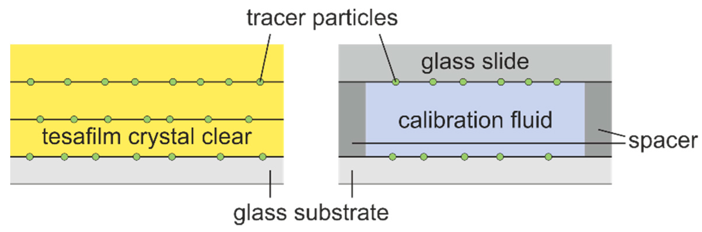
3.1. Focal Displacement Calibration

Initially, the focal displacement due to a mismatch between the immersion and sample refractive index was investigated. Calibration samples with different refractive indices were prepared and $z$-scans were carried out. A series of simulations with $z_p=0–200\mathsf{\mu }\mathrm{m}$ was performed for each sample using the optical properties of the objective and the measured substrate thickness as input parameters. Figure 5 shows a comparison of the best focus. The simulations (lines) show a very good agreement with the experimental results (markers) over a wide range of $n_s$, as do the data from our previous work [44]. The impact of the sample refractive index on the displacement can be determined from the slope, $m_d$, of the data. The following fit is based on simulations in the range of $n_s=1.0–1.7$:

$${\mathrm{m}}_{\mathrm{d}}=\frac{{\Delta \mathrm{z}}_{\mathrm{obj}}}{\Delta z_p}\approx 0.996\times {\mathrm{n}}_{\mathrm{s}}^{-1.056},R^2=1.00$$

(4)

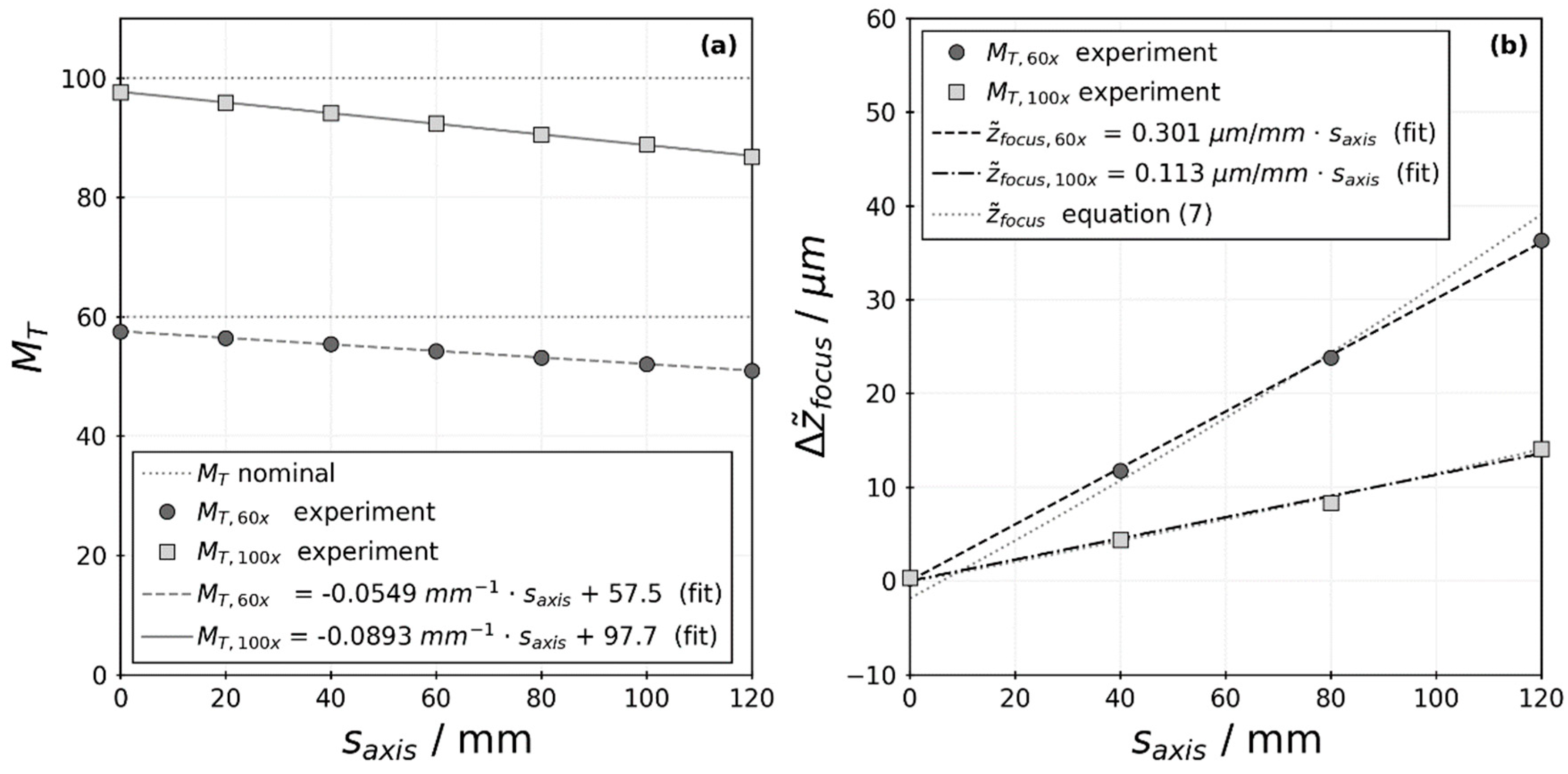
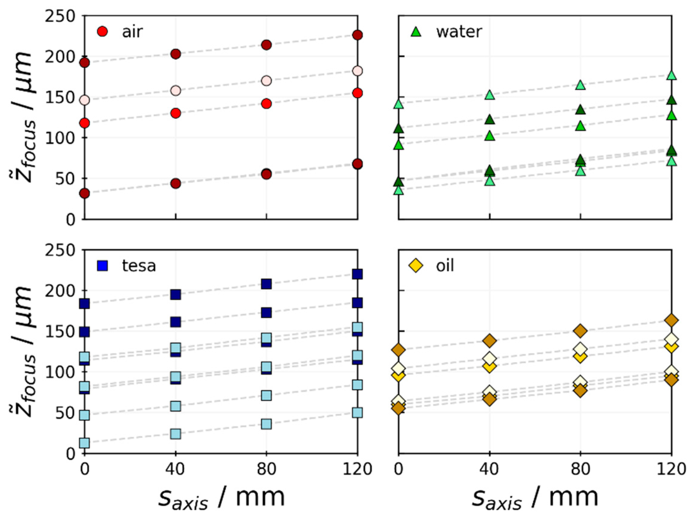
3.2. Experimental Calibration of Motorized Lens System

The multifocal setup introduces motorized lens systems uncommon in standard of-the-shelf microscopes. To compare the experimental ring sizes with the calculated PSFs, the transverse magnification was determined for different positions of the motorized lens. The experimental results indicate that even for $s_{axis}=0\mathrm{mm}$, the measured $M_T$ is slightly smaller than the nominal one imprinted on the objectives (Figure 6a). Furthermore, it can be clearly seen that the optical system is not telecentric, since the transverse magnification decreases with an increasing axial lens position.

The main purpose of the motorized lens system, however, is to change the focal plane position for each camera individually. Therefore, multiple calibration samples were scanned with different lens positions using the 60× objective. The best focus of each particle layer is depicted in Figure 7. Different color shades indicate individual samples. Data for each particle layer are connected with dashed gray lines for better readability. Each sample has an arbitrary origin of ${\tilde{z}}_{focus}$, which was kept constant for all lens positions. Therefore, only the slope of each dataset is of relevance. As shown, it is virtually identical for different particle layers within one sample as well as for different sample media, indicating that neither influences the focal shift due to the motorized lens.

An analytic solution can be derived from Equation (1). Considering that $\Delta {\tilde{z}}_{focus}$ is an axial distance in the object space and $\Delta s_{axis}$ is an axial displacement in the image space, the quotient is equivalent to the axial magnification, $M_L$ (Equation (5)). The negative sign needs to be introduced since an increase in ${\tilde{z}}_{focus}$ decreases the distance between the objective lens and the observed position [50]. Inserting the linear relation from Figure 6 (Equation (6)) and Equation (1) in (5), the subsequent integration yields Equation (7).

$$\frac{\Delta s_{axis}}{\Delta {\tilde{z}}_{focus}}=-M_L=\frac{d{s}_{axis}}{d{\tilde{z}}_{focus}}$$

(5)

$$M_T=m_T\times s_{axis}+b_T$$

(6)

$${\tilde{z}}_{focus}={\displaystyle \int }\frac{1}{-M_L}d{s}_{axis}={\displaystyle \int }\frac{1}{M_T^2}d{s}_{axis}=-\frac{1}{m_T\left(m_T·s_{axis}+b_T\right)}+c$$

(7)

By shifting the origin of ${\tilde{z}}_{focus}$ of the experimental datasets from Figure 7, the data coincide as depicted in Figure 6b. The dataset for the 100× objective was derived accordingly. The integration constant in (7) is fitted for each objective using the sum of least squares. For the 100× objective, the theory and experiment are in excellent agreement. For 60×, however, the theoretic solution deviates significantly from the experimental results. The reason for the deviation is most likely Equation (1), which is rigorously valid only for single thin lenses and not for complex lens systems as in microscope objectives. A linear fit is better suited to match the experimental data.

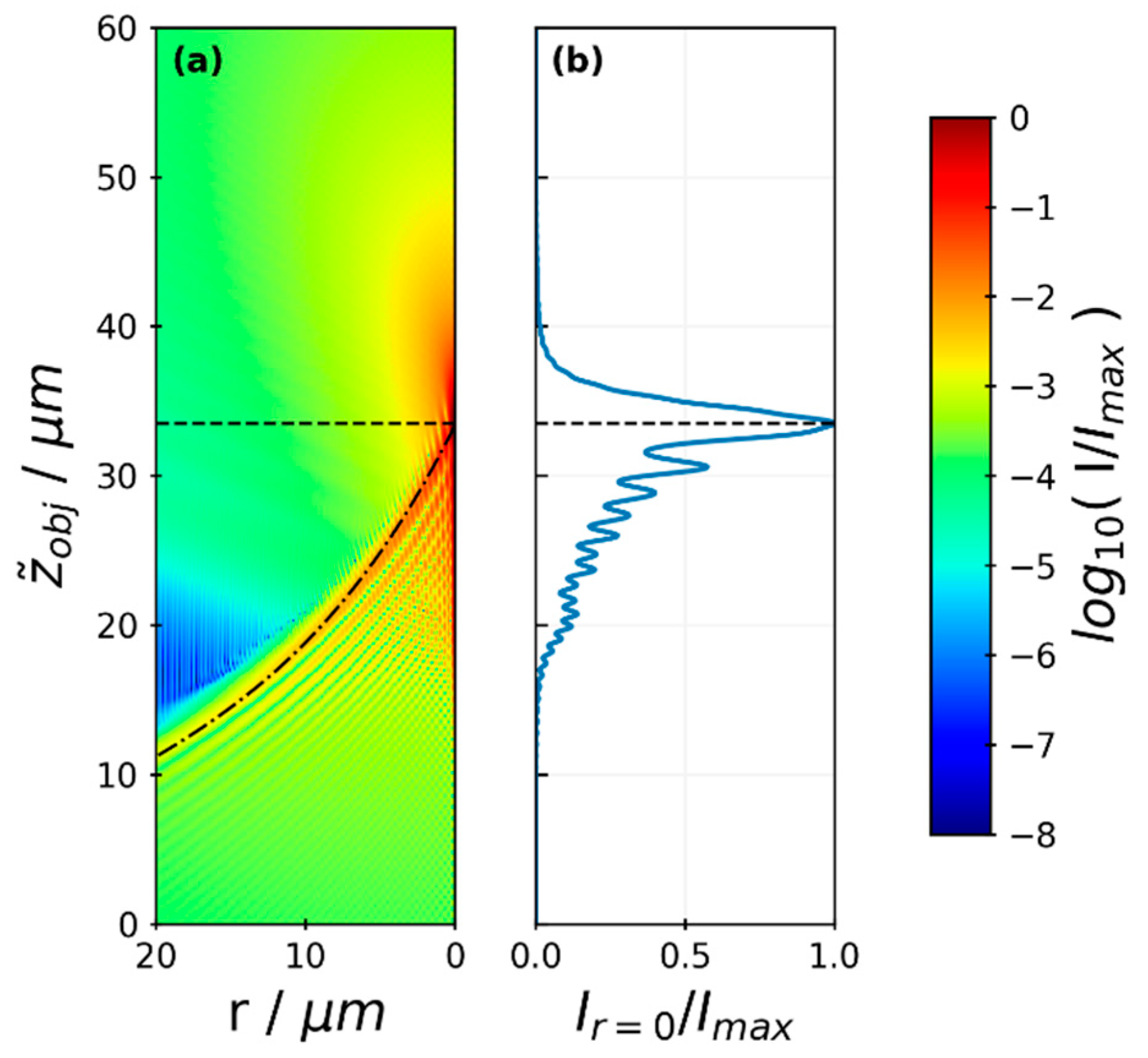
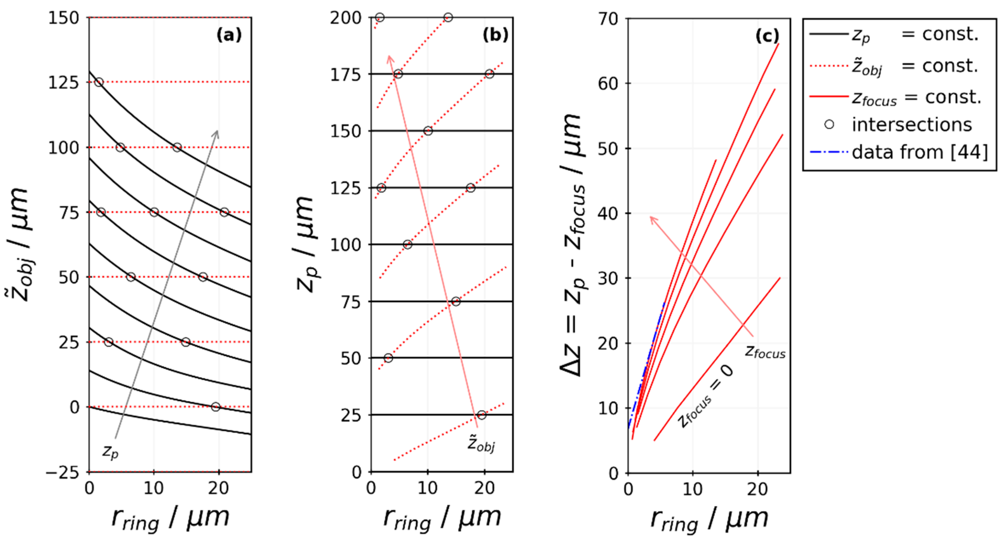
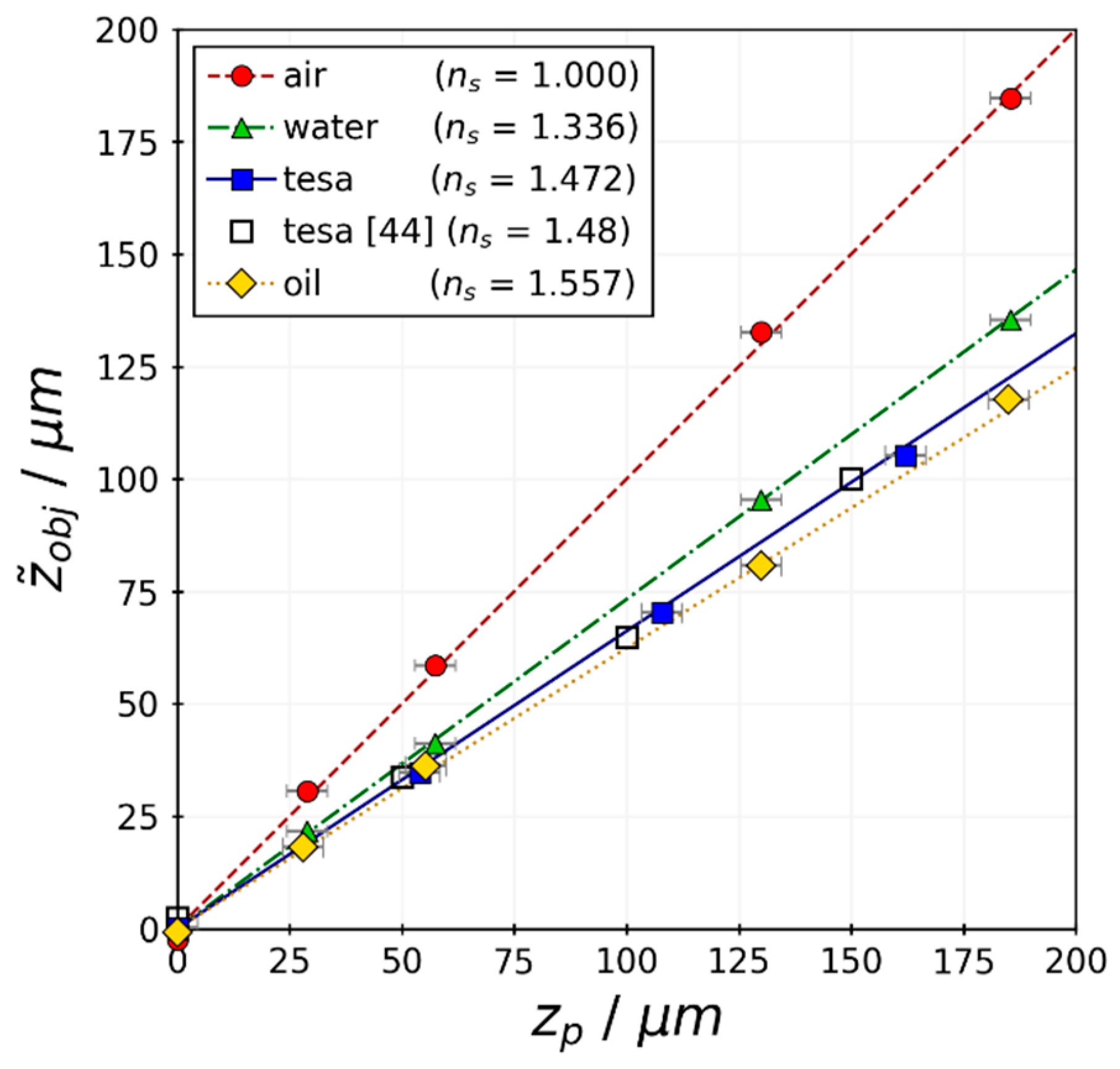
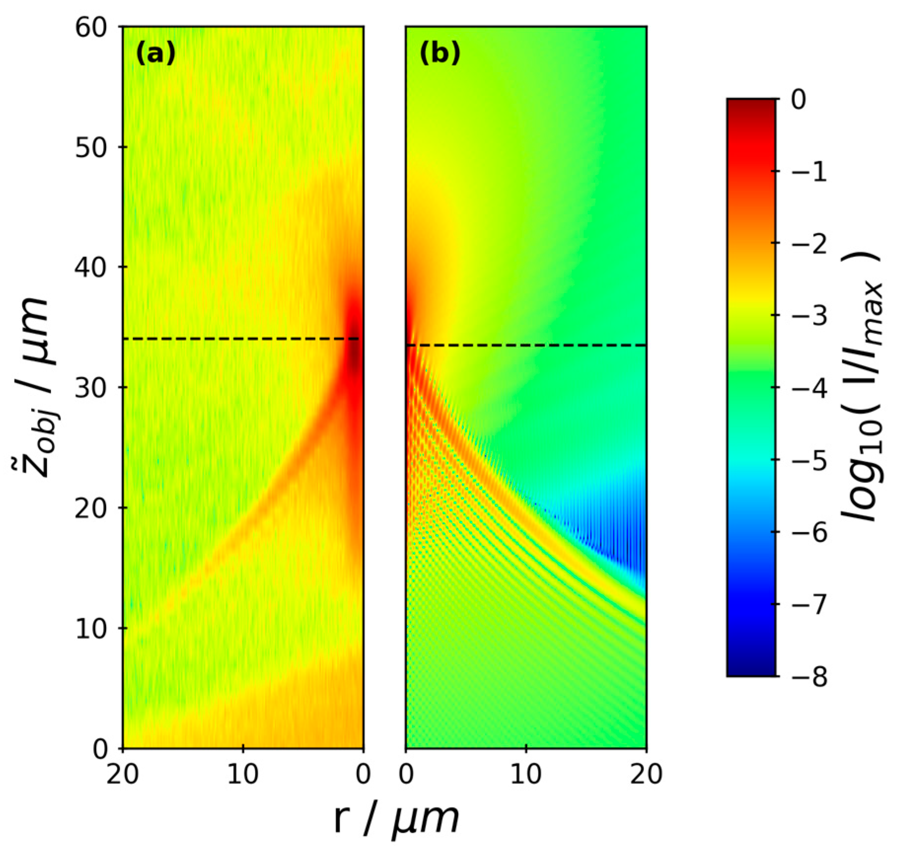
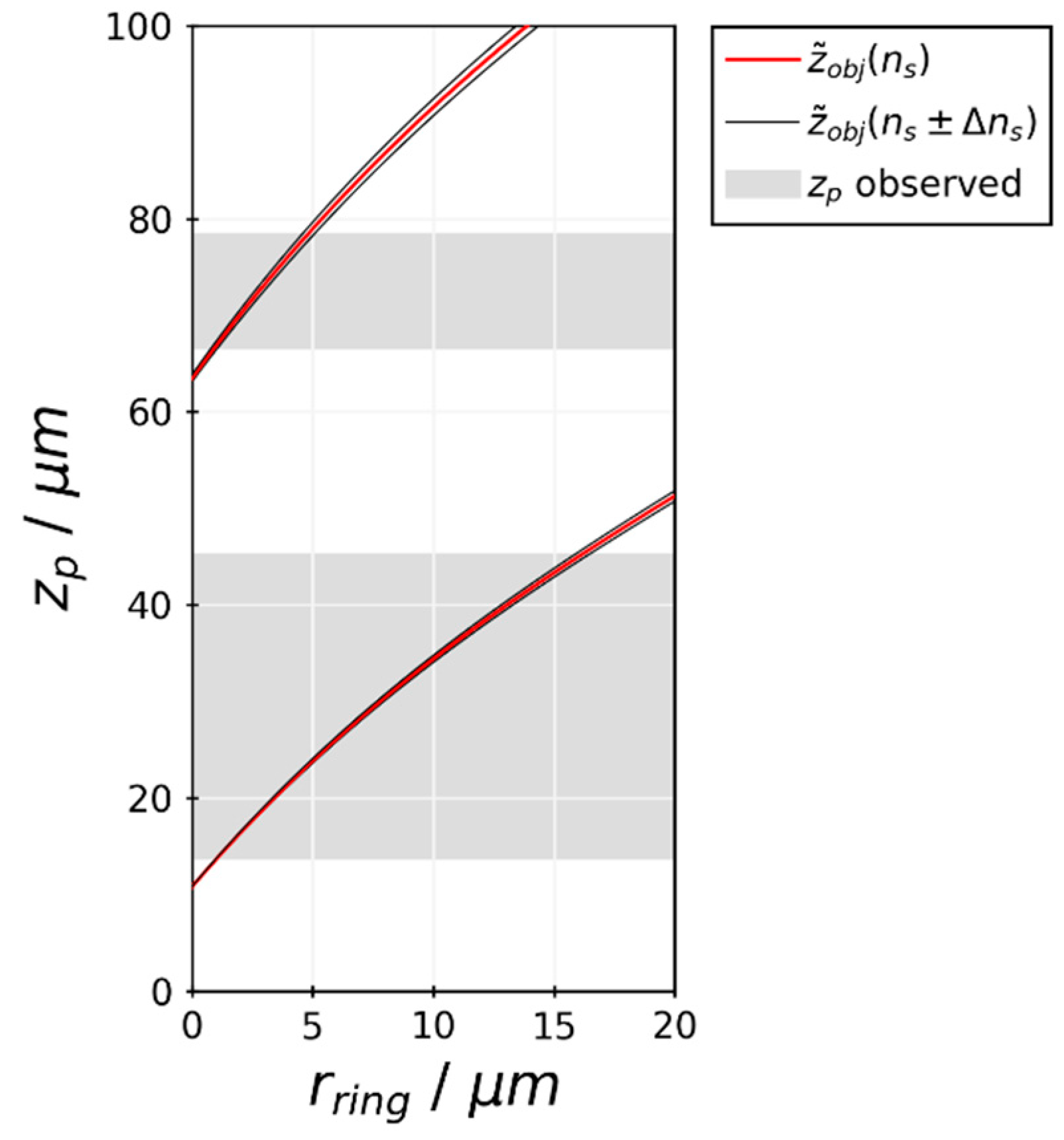
3.3. Diffraction-Ring Size Calibration for Off-Focus Particle Positions

Up to this point, only the best focus of the particles was considered. The axial position of particles is, however, determined from diffraction-ring sizes occurring whenever a particle is not in focus. With known transverse magnification, the radii of experimental PSFs derived from $z$-scans can be converted from image pixels to micrometers. A comparison with a simulated PSF is shown as a vertical cross-section in Figure 8. Overall, it shows a very good agreement despite the fact that the Gibson-Lanni simulation model assumes an ideal point source and the tracer particle has a diameter well above the pixel resolution limit of the cameras. With $M_T\left(s_{axis}=0\mathrm{mm}\right)=57.5$, the tracer particle diameter is $d_p=4.6\mathrm{px}$ and is clearly not an ideal point. As seen in Figure 8, this has no apparent effect on the PSF.

For quantitative validation of the simulation model regarding the ring sizes, a $z$-scan on a tesa stack was performed. The best focus and rings were detected via the vertical intensity profile and GPU-enhanced detection algorithm, respectively. Figure 9 shows the experimental results (markers) as well as the simulated ring sizes (red lines). The detection algorithm yields a high number of false-positive rings (blue crosses) for very small radii only. The deposition of the particle layers for the calibration samples was done from aqueous solution. The dry layers show a high amount of agglomerates, which tend to have a much higher intensity, resulting in a less pronounced blur-out. Drying experiments with polymer solutions do not suffer from tracer-particle agglomeration. Both the false positives as well as the detected agglomerates were sorted out manually, but are shown in Figure 9 for full disclosure. The quality of the detection algorithm, however, is not in the scope of this article.

Since experimental $z$-scans have an arbitrary origin, the detected best focus positions (dashed horizontal lines) were used to vertically shift the experimental results by calculating the sum of least squares with the best focus positions derived from simulations (dotted horizontal lines). Neither the distances between the individual particle layers nor the rings were fitted in any way. Figure 9 shows an excellent agreement between the experiments and simulations regarding the ring sizes for multiple settings of the cover-glass correction-collar ($t_g^{*}$). The actual substrate thickness was $t_g=144\mathsf{\mu }\mathrm{m}$. For a design value much larger than the actual value (see Figure 9c), the diffraction rings appear above the respective focal plane for the lower two particle layers and below for the upper two layers. This results in an area where a detected ring size is ambiguous regarding its corresponding particle position (i.e., the intersection of the red lines). For quantitative measurements, this ambiguity is unwanted and needs to be avoided.

Comparing the remaining two correction-collar settings, a change in the ring data’s slope is apparent (Figure 9a,b). Considering a smaller absolute slope, as observed for $t_g^{*}=150\mathsf{\mu }\mathrm{m}$, this setting would be beneficial if large errors in the detected ring radii are to be expected. A deviating ring size would have a less pronounced effect on the derived vertical particle position. The signal-to-noise ratio of the recorded rings decreases with an increasing ring size up to a point where ring detection is impossible. Considering a larger absolute slope, as observed for $t_g^{*}=110\mathsf{\mu }\mathrm{m}$, a ring with a constant diameter would have a larger distance to the corresponding focal plane if compared to $t_g^{*}=150\mathsf{\mu }\mathrm{m}$. Thus, if a large vertical observation volume is desired, a large absolute slope is beneficial. Overall, the correction-collar setting is a trade-off between the vertical extent of the observed volume and the error tolerance of ring size detection. We found that $t_g^{*}=110\mathsf{\mu }\mathrm{m}$ was most suitable for our application.

In [44], we reported data on ring-size calibration, plotted using the distance between the particle position and the focal plane. The simulated data in Figure 4c were derived using matching optical properties. A good agreement between the current simulations and our old data can be seen, but only for a single, large $z_{focus}$ position. Similar ring-size data can be found in [48,49,55,66]. Speidel et al. (2003) reported a linear relation between the ring-size and the distance to the focal plane, but they provided the ring radius in arbitrary units only [48]. The other authors reported non-linear relations [49,55,66]. Qualitatively, their data and shape of the plot compares well with our findings. However, a quantitative comparison with PSF simulations was not possible due to the lack of optical properties of the respective setups.

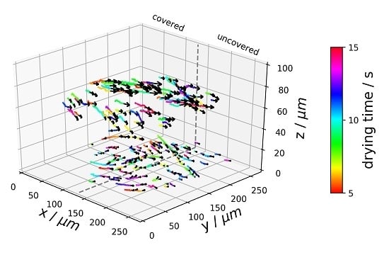
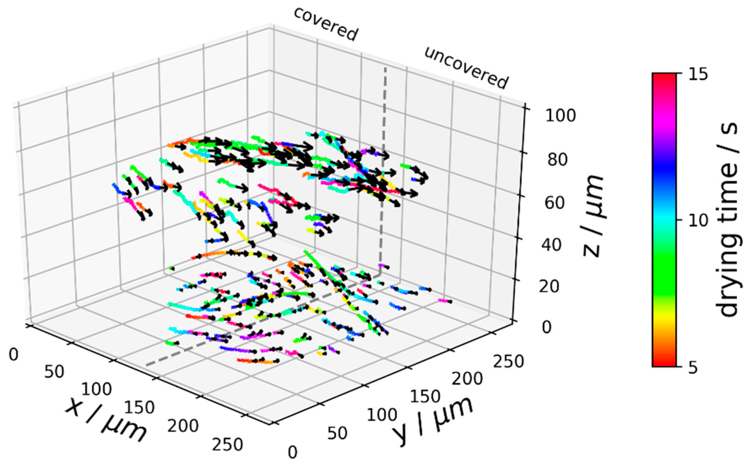
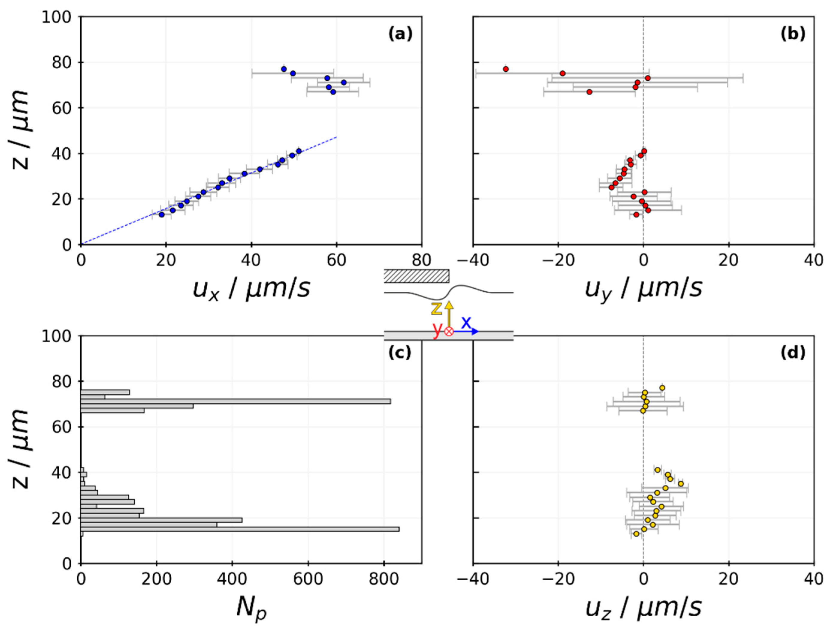
3.4. Flow Field of Partially Covered Drying Experiment

Recordings of both cameras from the drying experiment are provided in the Supplementary Materials. The dataset was evaluated as follows: Using the objective and lens positions and the linear fit in Figure 6b, the calculated focal planes were at ${\tilde{z}}_{obj,A,focus}=45.0\mathsf{\mu }\mathrm{m}$ and ${\tilde{z}}_{obj,B,focus}=8.3\mathsf{\mu }\mathrm{m}$ for the two cameras, respectively. The estimated sample refractive index was $n_s=1.374\pm 0.011$ during the observation period, including variations due to a vertical concentration gradient. With these input parameters, PSF simulations were performed and polynomial fit functions were derived as described in Figure 4a,b. Figure 10 shows the resulting lookup data, accounting for the uncertainty in $n_s$ and the focal planes of the two cameras. The transverse magnifications are $M_{T,A}=57.5$ and $M_{T,B}=50.8$, respectively. The gray area indicates the vertical field of view. It results from the minimal and maximal observed ring radius in the recordings. It is noteworthy that the significant concentration range the film undergoes within the observed timeframe results in only a small uncertainty of $n_s$. This is important, since $n_s$ has a major impact on $z_p$ calibration (see Figure 5). The range of uncertainty of $n_s$ is shown with black lines in Figure 10. The maximal error in the vertical particle position for the given experiment resulting from variations in $n_s$ are $\Delta z_{p,A,max}=\pm 0.7\mathsf{\mu }\mathrm{m}$ and $\Delta z_{p,B,max}=\pm 0.5\mathsf{\mu }\mathrm{m}$. $\Delta z_p$ increases with increasing $r_{ring}$ and increasing ${\tilde{z}}_{obj}$.

The resulting three-dimensional particle trajectories for both observation volumes are shown in Figure 11. The black arrows at the tip of each trajectory indicate the flow direction and velocity. It can be clearly seen that the dominant current is from the covered area towards the uncovered area. The colors indicate the temporal occurrence of particles. In this diagram, only the relative velocity of two trajectories with a similar length can be estimated by comparing the color gradient. A relatively smaller gradient on a trajectory of a similar length allows a conclusion on a higher velocity.

For quantitative assessment of the velocity, Savitzky-Golay filtering using the first derivate was applied to each trajectory. The results were averaged in slices of $\Delta z=2\mathsf{\mu }\mathrm{m}$ and for each cartesian velocity component. Figure 12 shows the vertical velocity distribution. The highest mean velocity occurs in the positive $x$ direction, from the covered to uncovered area. In (a), a vertical $x$-velocity gradient can be seen. This is to be expected for Marangoni convection, which is an interfacial flow. The viscosity of the polymer solution and the non-slip condition at the substrate results in the observed gradient. The in-plane velocity, $u_y$, perpendicular to $x$ is shown in (b). The mean velocity is small in the lower observation volume and scattered in the upper volume. The broad fluctuations at around $z=70\mathsf{\mu }\mathrm{m}$ indicate that averaging over the complete $xy$-domain might not be well suited if several different flow domains occur. Furthermore, it should be considered that tracer particles only provide Lagrangian information on the flow field. Considering the two upmost data points in (b), they indicate a negative mean y-velocity with moderate fluctuations. Considering the small number of averaged particles in these slices, as depicted in (c), the reason could be an uneven distribution or insufficient number of tracer particles. This may lead to a misinterpretation of the obtained data. An in-depth analysis of the flow regimes, however, is not in the scope of this article. The highest observed total velocity from quantitative µPTV is $u=84\mathsf{\mu }\mathrm{m}/\mathrm{s}$.

4. Discussion

It has been pointed out that despite more than a century of research on Marangoni convection, there is still a need for more quantitative experimental data. Past research efforts have been focused on convection patterns in pure liquids, omitting the complexity of superimposed solution drying. While often unwanted in functional thin films, surface deformation due to Marangoni flows may lead to homogeneous inkjet-printed patterns. The recently established measurement technique, µPTV, enables transient three-dimensional flow field measurements within thin films and small printed structures without obstructing the space above the sample. This facilitates the implementation of controlled drying boundary conditions. The calibration of such a setup is strongly dependent on optical parameters, such as the refractive index of the sample or the substrate glass thickness. We were able to demonstrate that our experimental calibration data are in very good agreement with simulated data from an existing, but recently accelerated, mathematical model, which relies only on the available data of the optical setup. Consequently, we derived polynomial functions from the simulation results, which can be used to match experimentally observed diffraction-ring sizes with vertical positions in the sample. In past research, experimental correlations between the ring diameter and the distance to the focal plane have been reported [48,49,55]. Due to a lack of data on the respective optical setups, a quantitative comparison could not be performed. Furthermore, we are the first to report a deliberate mismatch in the cover-glass correction collar settings to increase the axial field-of-view. The dependency of the lookup data on the sample refractive index is significant. Despite obvious concentration changes while drying the PVAc-MeOH solution at near ambient conditions, the refractive index within the observation period changes only slightly. This may vary for different material systems and drying conditions.

In previous work, PIV measurements resulted in two-dimensional qualitative flow field data where either only size and form of the convective cells were analyzed or velocities were derived only for a selected few representative particles. With a simple drying experiment, we demonstrated that µPTV measurements grant access to transient, three-dimensional microscopic flow fields, resulting in quantitative velocity data over a significant observation volume. As expected for a partially covered PVAc-MeOH film, the dominant flow occurs in the $x$-direction from the covered towards the uncovered area due to Marangoni convection (see Figure 12a). The $x$-velocity profile in the lower observation volume closer to the substrate appears to be linear and can be fitted accordingly as shown with a dashed blue line. Such a linear profile strongly resembles the flow profile of a planar Couette-flow, where a Newtonian fluid undergoes a shear-driven flow between a horizontally moving upper wall and a stationary lower wall. The resulting shear rate is $\Delta u_x/\Delta z=1.3{\mathrm{s}}^{-1}$, which is very low and justifies the assumption of Newtonian behavior for the PVAc-MeOH solution. Instead of a moving upper wall, however, the horizontal Marangoni flow from the covered towards the uncovered area acts as the driving force.

The velocities in the upper observation volume strongly deviate from a Couette-flow profile. Especially in the $y$-direction in the film plane, but perpendicular to the dominant $x$-flow, fluctuations increase drastically. This indicates a secondary instability, which needs to be investigated further in the near future. Errors induced by tracer particle sedimentation, inertia, and Brownian motion are discussed in detail in Appendix A. The sedimentation velocity is less than $1\mathsf{\mu }\mathrm{m}/\mathrm{h}$ while the observation period is $10\mathrm{s}$. Therefore, it is safe to assume that this has no noticeable impact on the results. However, Brownian motion may result in a velocity fluctuation of close to $1\mathsf{\mu }\mathrm{m}/\mathrm{s}$. Averaging multiple particle velocities significantly mitigates these undirected fluctuations. An axial extension of the observation volume would be beneficial and could be achieved by employing a high-power laser illumination.

5. Conclusions

Micro particle tracking velocimetry (µPTV) enables microfluidic flow-field measurements with only one optical access through a transparent substrate. The multifocal approach as well as the diffraction ring analysis allows for the detection of line-of-site velocities, resulting in a quantitative three-dimensional measurement technique. In this article, we have presented an in-depth calibration and evaluation routine for the line-of-site particle positions dependent on the optical parameters of the setup and the sample. Our experimental calibration data were in good agreement with a well-established simulation model. The unobstructed space above the sample makes µPTV ideal for the investigation of surface-tension driven convection in thin films and small printed structures, since the drying conditions can be adapted. This, as well as the evaluation routine, was successfully demonstrated on a simple drying experiment. In a partially covered thin film of poly(vinyl acetate)-methanol drying at near ambient conditions, a dominant flow from the covered towards the uncovered area was measured. The highest observed velocity with µPTV was $u=84\mathsf{\mu }\mathrm{m}/\mathrm{s}$. Fluctuations perpendicular to the dominant flow were detected and demand further investigations. Overall, we consider µPTV to be a useful addition to the existing portfolio of microfluidic measurement techniques.

References

1. Smith, P.J.; Stringer, J. Applications in Inkjet Printing. In Fundamentals of Inkjet Printing: The Science of Inkjet and Droplets; Hoath, S.D., Ed.; Wiley-VCH Verlag GmbH & Co. KGaA: Weinheim, Germany, 2016; pp. 397–418. ISBN 978-3-527-33785-9. [Google Scholar]
2. Deegan, R.D.; Bakajin, O.; Dupont, T.F.; Huber, G.; Nagel, S.R.; Witten, T.A. Capillary flow as the cause of ring stains from dried liquid drops. Nature 1997, 389, 827–829. [Google Scholar] [CrossRef]
3. Cavadini, P.; Krenn, J.; Scharfer, P.; Schabel, W. Investigation of surface deformation during drying of thin polymer films due to Marangoni convection. Chem. Eng. Process. 2013, 64, 24–30. [Google Scholar] [CrossRef]
4. Cavadini, P.; Erz, J.; Sachsenheimer, D.; Kowalczyk, A.; Willenbacher, N.; Scharfer, P.; Schabel, W. Investigation of the flow field in thin polymer films due to inhomogeneous drying. J. Coat. Technol. Res. 2015, 12, 921–926. [Google Scholar] [CrossRef]
5. Block, M.J. Surface Tension as the Cause of Bénard Cells and Surface Deformation in a Liquid Film. Nature 1956, 178, 650–651. [Google Scholar] [CrossRef]
6. Pearson, J.R.A. On convection cells induced by surface tension. J. Fluid Mech. 1958, 4, 489. [Google Scholar] [CrossRef]
7. Vanhook, S.J.; Schatz, M.F.; Swift, J.B.; McCormick, W.D.; Swinney, H.L. Long-wavelength surface-tension-driven Bénard convection: Experiment and theory. J. Fluid Mech. 1997, 345, 45–78. [Google Scholar] [CrossRef]
8. Yeo, L.Y.; Craster, R.V.; Matar, O.K. Marangoni instability of a thin liquid film resting on a locally heated horizontal wall. Phys. Rev. E 2003, 67, 56315. [Google Scholar] [CrossRef] [PubMed]
9. Bestehorn, M.; Pototsky, A.; Thiele, U. 3D Large scale Marangoni convection in liquid films. Eur. Phys. J. E Soft Matter 2003, 33, 457–467. [Google Scholar] [CrossRef] [Green Version]
10. Gambaryan-Roisman, T. Marangoni convection, evaporation and interface deformation in liquid films on heated substrates with non-uniform thermal conductivity. Int. J. Heat Mass Transf. 2010, 53, 390–402. [Google Scholar] [CrossRef]
11. Gambaryan-Roisman, T. Modulation of Marangoni convection in liquid films: Reinhard Miller, Honorary Issue. Adv. Colloid Interface Sci. 2015, 222, 319–331. [Google Scholar] [CrossRef] [PubMed]
12. Oron, A.; Davis, S.H.; Bankoff, S.G. Long-scale evolution of thin liquid films. Rev. Mod. Phys. 1997, 69, 931–980. [Google Scholar] [CrossRef]
13. Craster, R.V.; Matar, O.K. Dynamics and stability of thin liquid films. Rev. Mod. Phys. 2009, 81, 1131–1198. [Google Scholar] [CrossRef]
14. Chai, A.-T.; Zhang, N. Experimental study of Marangoni-Benard convection in a liquid layer induced by evaporation. Exp. Heat Transf. 1998, 11, 187–205. [Google Scholar] [CrossRef]
15. Merkt, D.; Bestehorn, M. Bénard–Marangoni convection in a strongly evaporating fluid. Physica D 2003, 185, 196–208. [Google Scholar] [CrossRef]
16. Sultan, E.; Boudaoud, A.; Amar, M.B. Evaporation of a thin film: Diffusion of the vapour and Marangoni instabilities. J. Fluid Mech. 2005, 543, 183. [Google Scholar] [CrossRef]
17. Doumenc, F.; Boeck, T.; Guerrier, B.; Rossi, M. Transient Rayleigh–Bénard–Marangoni convection due to evaporation: A linear non-normal stability analysis. J. Fluid Mech. 2010, 648, 521. [Google Scholar] [CrossRef]
18. Chauvet, F.; Dehaeck, S.; Colinet, P. Threshold of Bénard-Marangoni instability in drying liquid films. Europhys. Lett. 2012, 99, 34001. [Google Scholar] [CrossRef] [Green Version]
19. Kanatani, K. Effects of convection and diffusion of the vapour in evaporating liquid films. J. Fluid Mech. 2013, 732, 128–149. [Google Scholar] [CrossRef]
20. Bormashenko, E.; Pogreb, R.; Stanevsky, O.; Bormashenko, Y.; Tamir, S.; Cohen, R.; Nunberg, M.; Gaisin, V.-Z.; Gorelik, M.; Gendelman, O.V. Mesoscopic and submicroscopic patterning in thin polymer films: Impact of the solvent. Mater. Lett. 2005, 59, 2461–2464. [Google Scholar] [CrossRef]
21. Bormashenko, E.; Pogreb, R.; Stanevsky, O.; Bormashenko, Y.; Gendelman, O. Formation of honeycomb patterns in evaporated polymer solutions: Influence of the molecular weight. Mater. Lett. 2005, 59, 3553–3557. [Google Scholar] [CrossRef]
22. Bormashenko, E.; Pogreb, R.; Musin, A.; Stanevsky, O.; Bormashenko, Y.; Whyman, G.; Gendelman, O.; Barkay, Z. Self-assembly in evaporated polymer solutions: Influence of the solution concentration. J. Colloid Interface Sci. 2006, 297, 534–540. [Google Scholar] [CrossRef] [PubMed]
23. Toussaint, G.; Bodiguel, H.; Doumenc, F.; Guerrier, B.; Allain, C. Experimental characterization of buoyancy- and surface tension-driven convection during the drying of a polymer solution. Int. J. Heat Mass Transf. 2008, 51, 4228–4237. [Google Scholar] [CrossRef]
24. Bormashenko, E.; Pogreb, R.; Stanevsky, O.; Bormashenko, Y.; Stein, T.; Gendelman, O.; Gengelman, O. Mesoscopic patterning in evaporated polymer solutions: New experimental data and physical mechanisms. Langmuir 2005, 21, 9604–9609. [Google Scholar] [CrossRef] [PubMed]
25. Kumacheva, E.; Li, L.; Winnik, M.A.; Shinozaki, D.M.; Cheng, P.C. Direct Imaging of Surface and Bulk Structures in Solvent Cast Polymer Blend Films. Langmuir 1997, 13, 2483–2489. [Google Scholar] [CrossRef]
26. Bormashenko, E.; Balter, S.; Pogreb, R.; Bormashenko, Y.; Gendelman, O.; Aurbach, D. On the mechanism of patterning in rapidly evaporated polymer solutions: Is temperature-gradient-driven Marangoni instability responsible for the large-scale patterning? J. Colloid Interface Sci. 2010, 343, 602–607. [Google Scholar] [CrossRef] [PubMed]
27. Wang, J.-M.; Liu, G.-H.; Fang, Y.-L.; Li, W.-K. Marangoni effect in nonequilibrium multiphase system of material processing. Rev. Chem. Eng. 2016, 32, 2. [Google Scholar] [CrossRef]
28. Larson, R.G. Transport and deposition patterns in drying sessile droplets. AIChE J. 2014, 60, 1538–1571. [Google Scholar] [CrossRef] [Green Version]
29. Anyfantakis, M.; Baigl, D. Manipulating the Coffee-Ring Effect: Interactions at Work. ChemPhysChem 2015, 16, 2726–2734. [Google Scholar] [CrossRef] [PubMed]
30. Sun, J.; Bao, B.; He, M.; Zhou, H.; Song, Y. Recent Advances in Controlling the Depositing Morphologies of Inkjet Droplets. ACS Appl. Mater. Interfaces 2015. [Google Scholar] [CrossRef] [PubMed]
31. Hu, H.; Larson, R.G. Marangoni effect reverses coffee-ring depositions. J. Phys. Chem. B 2006, 110, 7090–7094. [Google Scholar] [CrossRef] [PubMed]
32. De Gans, B.-J.; Duineveld, P.C.; Schubert, U.S. Inkjet Printing of Polymers: State of the Art and Future Developments. Adv. Mater. 2004, 16, 203–213. [Google Scholar] [CrossRef]
33. Poulard, C.; Damman, P. Control of spreading and drying of a polymer solution from Marangoni flows. Europhys. Lett. 2007, 80, 64001. [Google Scholar] [CrossRef]
34. Kajiya, T.; Doi, M. Dynamics of Drying Process of Polymer Solution Droplets: Analysis of Polymer Transport and Control of Film Profiles. Nihon Reoroji Gakk. 2011, 39, 17–28. [Google Scholar] [CrossRef] [Green Version]
35. Trantum, J.R.; Baglia, M.L.; Eagleton, Z.E.; Mernaugh, R.L.; Haselton, F.R. Biosensor design based on Marangoni flow in an evaporating drop. Lab Chip 2014, 14, 315–324. [Google Scholar] [CrossRef] [PubMed]
36. Zhang, Y.; Yang, S.; Chen, L.; Evans, J.R.G. Shape changes during the drying of droplets of suspensions. Langmuir 2008, 24, 3752–3758. [Google Scholar] [CrossRef] [PubMed]
37. Majumder, M.; Rendall, C.S.; Eukel, J.A.; Wang, J.Y.L.; Behabtu, N.; Pint, C.L.; Liu, T.-Y.; Orbaek, A.W.; Mirri, F.; Nam, J.; et al. Overcoming the “coffee-stain” effect by compositional Marangoni-flow-assisted drop-drying. J. Phys. Chem. B 2012, 116, 6536–6542. [Google Scholar] [CrossRef] [PubMed]
38. Babatunde, P.O.; Hong, W.J.; Nakaso, K.; Fukai, J. Effect of Solute- and Solvent-Derived Marangoni Flows on the Shape of Polymer Films Formed from Drying Droplets. AIChE J. 2013, 59, 699–702. [Google Scholar] [CrossRef]
39. Jafari Kang, S.; Vandadi, V.; Felske, J.D.; Masoud, H. Alternative mechanism for coffee-ring deposition based on active role of free surface. Phys. Rev. E 2016, 94, 63104. [Google Scholar] [CrossRef] [PubMed]
40. Kang, Q.; Zhang, J.F.; Hu, L.; Duan, L. Experimental study on Benard-Marangoni convection by PIV and TCL. Proc. SPIE 2003, 5058, 155. [Google Scholar] [CrossRef]
41. Kang, K.H.; Lee, S.J.; Lee, C.M.; Kang, I.S. Quantitative visualization of flow inside an evaporating droplet using the ray tracing method. Meas. Sci. Technol. 2004, 15, 1104–1112. [Google Scholar] [CrossRef]
42. Kaneda, M.; Hyakuta, K.; Takao, Y.; Ishizuka, H.; Fukai, J. Internal Flow in Polymer Solution Droplets Deposited on a Lyophobic Surface during a Receding Process. Langmuir 2008, 24, 9102–9109. [Google Scholar] [CrossRef] [PubMed]
43. Bassou, N.; Rharbi, Y. Role of Bénard-Marangoni instabilities during solvent evaporation in polymer surface corrugations. Langmuir 2009, 25, 624–632. [Google Scholar] [CrossRef] [PubMed]
44. Cavadini, P.; Weinhold, H.; Tönsmann, M.; Chilingaryan, S.; Kopmann, A.; Lewkowicz, A.; Miao, C.; Scharfer, P.; Schabel, W. Investigation of the flow structure in thin polymer films using 3D µPTV enhanced by GPU. Exp. Fluids 2018, 59, 370. [Google Scholar] [CrossRef]
45. Lindken, R.; Rossi, M.; Grosse, S.; Westerweel, J. Micro-Particle Image Velocimetry (microPIV): Recent developments, applications, and guidelines. Lab Chip 2009, 9, 2551–2567. [Google Scholar] [CrossRef] [PubMed]
46. Wereley, S.T.; Meinhart, C.D. Recent Advances in Micro-Particle Image Velocimetry. Annu. Rev. Fluid Mech. 2010, 42, 557–576. [Google Scholar] [CrossRef]
47. Cierpka, C.; Kähler, C.J. Particle imaging techniques for volumetric three-component (3D3C) velocity measurements in microfluidics. J. Vis. 2012, 15, 1–31. [Google Scholar] [CrossRef]
48. Speidel, M.; Jonáš, A.; Florin, E.-L. Three-dimensional tracking of fluorescent nanoparticles with subnanometer precision by use of off-focus imaging. Opt. Lett. 2003, 28, 69. [Google Scholar] [CrossRef] [PubMed]
49. Wu, M.; Roberts, J.W.; Buckley, M. Three-dimensional fluorescent particle tracking at micron-scale using a single camera. Exp. Fluids 2005, 38, 461–465. [Google Scholar] [CrossRef]
50. Hecht, E. Optics, 5th ed.; Pearson: Boston, MA, USA; Columbus, OH, USA; Indianapolis, IN, USA, 2017; ISBN 0-133-97722-6. [Google Scholar]
51. Gross, H. Handbook of Optical Systems. In Fundamentals of Technical Optics, 1st ed., 2nd repr.; Wiley-VCH: Weinheim, Germany, 2011; Volume 1, ISBN 3-527-40377-9. [Google Scholar]
52. Gibson, S.F.; Lanni, F. Experimental test of an analytical model of aberration in an oil-immersion objective lens used in three-dimensional light microscopy. J. Opt. Soc. Am. A 1992, 9, 154. [Google Scholar] [CrossRef] [PubMed]
53. Li, J.; Xue, F.; Blu, T. Fast and accurate three-dimensional point spread function computation for fluorescence microscopy. J. Opt. Soc. Am. A 2017, 34, 1029–1034. [Google Scholar] [CrossRef] [PubMed]
54. Hell, S.; Reiner, G.; Cremer, C.; Stelzer, E.H.K. Aberrations in confocal fluorescence microscopy induced by mismatches in refractive index. J. Microsc. 1993, 169, 391–405. [Google Scholar] [CrossRef]
55. Afik, E. Robust and highly performant ring detection algorithm for 3d particle tracking using 2d microscope imaging. Sci. Rep. 2015, 5, 13584. [Google Scholar] [CrossRef] [PubMed] [Green Version]
56. Ciddor, P.E. Refractive index of air: New equations for the visible and near infrared. Appl. Opt. 1996, 35, 1566–1573. [Google Scholar] [CrossRef] [PubMed]
57. Daimon, M.; Masumura, A. Measurement of the refractive index of distilled water from the near-infrared region to the ultraviolet region. Appl. Opt. 2007, 46, 3811. [Google Scholar] [CrossRef] [PubMed]
58. Schabel, W. Trocknung von Polymerfilmen. Messung von Konzentrationsprofilen mit der Inversen-Mikro-Raman-Spektroskopie. Ph.D. Thesis, University of Karlsruhe, Karlsruhe, Germany, Shaker, Aachen, Germany, 2004. [Google Scholar]
59. Tasic, A.Z.; Djordjevic, B.D.; Grozdanic, D.K.; Radojkovic, N. Use of mixing rules in predicting refractive indexes and specific refractivities for some binary liquid mixtures. J. Chem. Eng. Data 1992, 37, 310–313. [Google Scholar] [CrossRef]
60. Siebel, D.K. Zur Mehrkomponentendiffusion in Polymer-Lösemittel-Systemen. Untersuchungen im Kontext der Polymerfilmtrocknung mittels inverser Mikro-Raman-Spektroskopie. Ph.D. Thesis, Karlsruhe Institute of Technology (KIT), Karlsruhe, Germany, Verlag Dr. Hut., München, Germany, 2017. [Google Scholar]
61. Erz, J. In-situ Visualisierung von Oberflächendeformationen aufgrund von Marangoni-Konvektion während der Filmtrocknung. Ph.D. Thesis, Karlsruhe Institute of Technology (KIT), Karlsruhe, Germany, KIT Scientific Publ., Karlsruhe, Germany, 2014. [Google Scholar]
62. VDI e.V. (Ed.) VDI-Wärmeatlas, 11th ed.; Springer Vieweg: Berlin, Germany, 2013; ISBN 978-3-642-19980-6. [Google Scholar]
63. García-Mardones, M.; Cea, P.; López, M.C.; Lafuente, C. Refractive properties of binary mixtures containing pyridinium-based ionic liquids and alkanols. Thermochim. Acta 2013, 572, 39–44. [Google Scholar] [CrossRef]
64. Afik, E.; Steinberg, V. On the role of initial velocities in pair dispersion in a microfluidic chaotic flow. Nat. Commun. 2017, 8, 468. [Google Scholar] [CrossRef] [PubMed]
65. Savitzky, A.; Golay, M.J.E. Smoothing and Differentiation of Data by Simplified Least Squares Procedures. Anal. Chem. 1964, 36, 1627–1639. [Google Scholar] [CrossRef]
66. Park, J.S.; Kihm, K.D. Three-dimensional micro-PTV using deconvolution microscopy: Experiments in Fluids. Exp. Fluids 2006, 40, 491–499. [Google Scholar] [CrossRef]
67. Raffel, M.; Willert, C.E.; Kompenhans, J. Particle Image Velocimetry: A Practical Guide; Springer: Berlin/Heidelberg, Germany, 1998; ISBN 978-3-662-03639-6. [Google Scholar]
68. Santiago, J.G.; Wereley, S.T.; Meinhart, C.D.; Beebe, D.J.; Adrian, R.J. A particle image velocimetry system for microfluidics: Experiments in Fluids. Exp. Fluids 1998, 25, 316–319. [Google Scholar] [CrossRef]
69. Taylor, J.R. An Introduction to Error Analysis: The Study of Uncertainties in Physical Measurements, 2nd ed.; University Science Books: Sausalito, CA, USA, 1997; ISBN 978-0935702422. [Google Scholar]
Figure 1. Outline of micro particle tracking velocimetry (µPTV). The objective lens is attached to a piezo positioner. The signal is distributed to up to five cameras using beam splitters. Motorized lens systems precede four out of five cameras. (a) The complete setup. (b) Complete optical setup of a single camera. For reasons of clarity, only one camera system is depicted in full.
Colloids 03 00039 g001
Figure 2. Exemplary asymmetric PSF simulated with the Gibson-Lanni mode implementation by Li et al. (2017) [53]. Parameters: z p = 54   μ m , n s = 1.472 , N A = 0.95 , t g * = 150   μ m , t g = 144   μ m . (a) Vertical cross-section of PSF. The dash-dotted line indicates the outmost ring smoothened by a polynomial fit of 4th degree. (b) Axial intensity profile. The dashed line indicates the best focus at z ˜ o b j = 33.5   μ m .
Colloids 03 00039 g002
Figure 3. Schematic drawings of the calibration samples used for detecting tracer particles with known positions and a known sample refractive index. (Left) Tesa stack; (Right) Glass slides with spacers and calibration fluid.
Colloids 03 00039 g003
Figure 4. Conversion steps to obtain particle-position fit functions from simulations: (a) Ring sizes for various particle positions ( z p ) and intersections for constant objective positions. (b) Particle positions as a polynomial function of the ring sizes for various objective positions derived from intersections in (a). (c) Particle distance to the focal plane depending on the ring sizes and focal plane position derived from (b) with Equation (2), including the experimental fit from [44].
Colloids 03 00039 g004
Figure 5. Focal displacement due to mismatch in the refractive indices of immersion (air, n i = 1.000 ) and sample media ( n s ). Points indicate experimental values from the calibration samples; lines indicate simulations.
Colloids 03 00039 g005
Figure 6. Experimental calibration of the magnification. (a) Dependency of the transverse magnification ( M T ) on the position of the motorized lens ( s a x i s ) for two objectives with different nominal magnification. Experimental values and linear fit. (b) Axial focal displacement as a function of the motorized lens position. Theoretical trend for thin lenses (dotted line), experimental results (points), and linear fit (dashed/dash dotted lines).
Colloids 03 00039 g006
Figure 7. Axial focal displacement as a function of the motorized lens position derived from the z -scans of calibration samples with a 60× objective. Different color shades indicate individual samples. Data for each particle layer are connected with dashed gray lines for better readability. Each sample has an arbitrary origin of z ˜ f o c u s , which remains constant within individual datasets.
Colloids 03 00039 g007
Figure 8. Vertical cross-section of the PSF from a single tracer particle. Parameters: z p = 54   μ m , n s = 1.472 , N A = 0.95 , t g * = 150   μ m , t g = 144   μ m . (a) Experimental result from a z -scan on a tesa calibration sample. Cross-section image stitched with ImageJ. (b) Simulation with fast Gibson-Lanni model implementation [53]. Dashed line indicates the best focus at z ˜ o b j , e x p = 34   μ m and z ˜ o b j , s i m = 33.5   μ m , respectively.
Colloids 03 00039 g008
Figure 9. Comparison of experimental and simulated diffraction ring sizes in a tesa stack for different cover-glass correction-collar settings, t g * . Experimental data were shifted vertically to match best with the simulated focal plane positions. Ring sizes were not fitted in any way.
Colloids 03 00039 g009
Figure 10. Calibration function chart derived from PSF simulations with input parameters from the partially covered drying experiment. Estimated parameters: n s = 1.374 ± 0.011 . Parameters from the experimental setup: z ˜ o b j , A = 45.0   μ m , z ˜ o b j , B = 8.3   μ m . Experimental observations: r r i n g , A , m i n = 0.9   μ m , r r i n g , A , m a x = 4.8   μ m , r r i n g , B , m i n = 1.0   μ m , r r i n g , B , m a x = 16.2   μ m .
Colloids 03 00039 g010
Figure 11. Detected particle trajectories in PVAc-MeOH during a drying experiment with partially covered film. Tracks with six or less particle positions observed in consecutive frames were omitted for reasons of clarity. Black arrows at the end of each trajectory indicate the flow direction smoothed with the Savitzky-Golay filter.
Colloids 03 00039 g011
Figure 12. Cartesian velocity components from a partially covered drying experiment. The velocities of multiple particles were averaged in slices of Δ z = 2   μ m . Error bars indicate the standard deviation. (a) Mean x -velocity component as a function of the vertical position. Dashed blue line indicates a linear fit resembling a Couette-flow profile. (b,d) Mean y - and z -velocity component, respectively, as a function of the vertical position. (c) Number of particles, N p , averaged in each slice.
Colloids 03 00039 g012