Improving Graph-Based Sleep Staging with Shared Waveform Node Representations

Abstract

Graph-based sleep-staging models use different node representations, making it difficult to separate the contribution of the frontend from that of the graph architecture. We investigate whether a common raw-waveform encoder can improve heterogeneous graph models without model- or dataset-specific architectural tuning. We replace the Native frontends of five graph backbones with the same compact one-dimensional convolutional neural network (CNN). The CNN learns node representations directly from 30 s polysomnographic waveforms, while each model retains its original graph-construction mechanism, temporal context, and prediction modules. Three training strategies are compared across five datasets using matched five-fold subject-wise cross-validation: two-stage training (CNN–2S), end-to-end training (CNN–E2E), and pretraining followed by fine-tuning (CNN–PTFT). At least one CNN strategy outperforms the corresponding Native frontend in 22 of the 25 backbone–dataset combinations. Mean macro-F1 gains are 2.99, 2.34, and 2.53 percentage points for CNN–2S, CNN–E2E, and CNN–PTFT, respectively. Gains are positive on average for all sleep stages and are largest for N1 and REM. CNN–2S gives the strongest overall results and the most favorable aggregate performance–cost balance, although the effect on training time varies across backbones. The frozen CNN–2S representation also remains effective when transferred across datasets. The findings support node-representation learning as an important component of graph-based sleep-staging design.

1. Introduction

Sleep staging is a central component of clinical sleep assessment and sleep research. In standard practice, a polysomnographic (PSG) recording is divided into 30 s epochs, and each epoch is assigned to wakefulness (W), one of three non-rapid-eye-movement stages (N1–N3), or rapid-eye-movement (REM) sleep [1]. Reliable staging requires both local physiological evidence and temporal context. Within an epoch, electroencephalogram (EEG), electrooculography (EOG), and submental electromyography (EMG) signals contain complementary stage-related patterns, including changes in background rhythm, slow waves, spindles, K-complexes, eye movements, and muscle tone. At the same time, sleep evolves through structured transitions, making neighboring epochs informative when the target epoch is ambiguous. N1 is a clear example: it is transitional, comparatively rare, and less consistently identified even by expert scorers [1,2].

Modern neural systems increasingly learn representations directly from raw EEG or PSG signals while also modeling temporal dependencies across sleep epochs. Early influential architectures combined convolutional feature extraction with recurrent or sequence modeling [3,4,5,6,7]. Later work expanded temporal modeling through longer sequence contexts and through attention and transformer architectures [8,9,10]. More recent developments include transformer models designed for flexible multichannel PSG, large-scale pretrained sleep representations, and approaches targeting generalization across datasets and recording configurations, reflecting a broader shift toward representations that can be reused across channels, cohorts, and downstream tasks [11,12,13,14,15,16].

Graph neural networks offer a complementary inductive bias for multichannel PSG by representing channels as nodes and their anatomical, functional, or learned relations as edges. GraphSleepNet learns an adaptive functional graph and combines graph convolution with spatial–temporal attention [17]. MSTGCN adds a coordinate-based graph view and adversarial domain generalization [18], whereas ProductGraphSleepNet learns spatial and temporal factor graphs [19]. JK-STGCN combines functional and temporal-information graphs through jumping connections [20], and STDP-GCN constructs directed channel relations from spike timing [21]. Other graph-based sleep-staging approaches have explored self-attention graphs, multi-branch graph-convolutional fusion, and attention-based spatial–temporal graph modeling [22,23,24]. The five models considered in this study therefore represent distinct graph-design principles, spanning adaptive, multi-view, product, jumping-knowledge, and spike-derived constructions.

These models differ not only in their graph structures but also in how they encode PSG signals before graph processing. GraphSleepNet and ProductGraphSleepNet use nine differential-entropy (DE) features per channel, MSTGCN and JK-STGCN first train a two-branch convolutional FeatureNet, and STDP-GCN combines a spike-derived graph with spectral features computed from the residual waveform. More broadly, the choice of data representation can substantially influence time-series classification performance [25]. Because these graph models were developed together with different representation pipelines, the contribution of the node representation is difficult to separate from that of the graph architecture itself. This heterogeneity raises a simple question: can the same learned raw-waveform encoder improve graph models built on different feature representations and graph-learning principles?

We address this question by replacing each model’s original node representation with the same compact one-dimensional CNN trunk while retaining its graph construction, graph convolution, temporal context, and prediction modules. The same convolutional architecture is used across all backbones and datasets, without configuration-specific architectural tuning. We compare three training strategies: supervised epoch-level pretraining followed by a frozen graph stage (CNN–2S), joint training from random initialization (CNN–E2E), and pretraining followed by joint fine-tuning (CNN–PTFT). The resulting four frontend conditions, including the reproduced Native frontend, are evaluated for five graph backbones on five prepared dataset configurations. This provides a common experimental setting for examining the effect of frontend replacement across heterogeneous graph models. The contribution of this study is therefore a controlled evaluation of node-representation learning across established graph architectures, using a shared waveform frontend.

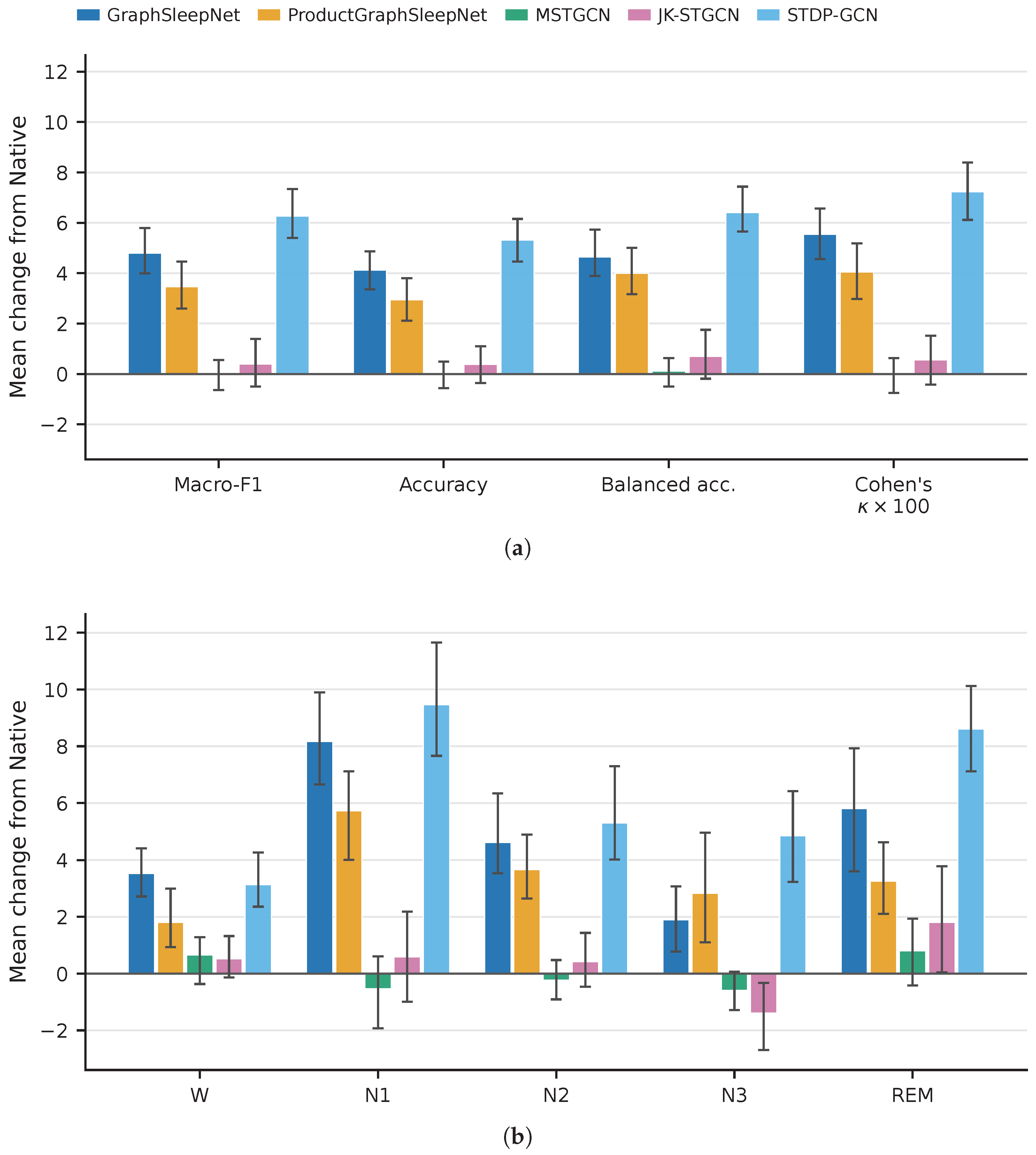
The results show a recurring benefit from replacing the Native frontend with the learned waveform representation. The best CNN regime outperforms the matching Native condition in 22 of the 25 backbone–dataset combinations. Across the complete grid, two-stage training increases mean macro-F1 by 2.99 percentage points, while end-to-end training and pretraining followed by fine-tuning yield gains of 2.34 and 2.53 points, respectively. The most consistent improvements are observed for models whose Native frontends rely on fixed spectral representations. Gains are positive on average for every sleep stage and are largest for N1 and REM. The normalization controls show that the gains are not explained by waveform z-scoring alone and are retained when later epochs are excluded from the normalization statistics. The two-stage encoder also remains effective when transferred across datasets. In the fixed-graph analysis, most of the improvement is retained when the Native graph is held fixed. Together, these findings support treating node-representation learning as an explicit part of graph-based sleep-staging design.

2. Materials and Methods

2.1. Study Design and Problem Formulation

Let N be the number of PSG channels and let ${\mathbf{s}}_{t,n}\in {\mathbb{R}}^L$ denote the 30 s waveform of channel $n\in \{1,\dots ,N\}$ during epoch t, sampled at 100 Hz, with $L=3000$ samples. The corresponding multichannel epoch ${\mathbf{S}}_t$ is

$${\mathbf{S}}_t={[{\mathbf{s}}_{t,1},\dots ,{\mathbf{s}}_{t,N}]}^{\top }\in {\mathbb{R}}^{N\times L}.$$

Each epoch has a sleep-stage label $y_t\in \mathcal{Y}$, where

$$\mathcal{Y}=\{\mathrm{W},\mathrm{N}1,\mathrm{N}2,\mathrm{N}3,\mathrm{REM}\}.$$

Let m index an evaluated graph backbone. Backbone m uses an odd-length context ${\mathcal{C}}_t^{\left(m\right)}$ of length $T_m$,

$${\mathcal{C}}_t^{\left(m\right)}=({\mathbf{S}}_{t-d_m},\dots ,{\mathbf{S}}_{t+d_m}),T_m=2d_m+1,$$

to predict the stage $y_t$ of its center epoch, where $d_m$ is the number of neighboring epochs included on either side.

Each channel and epoch is represented at the graph-model interface by a node vector ${\mathbf{x}}_{t,n}\in {\mathbb{R}}^{F_m}$, where $F_m$ is the node-feature width required by backbone m. We compare the reproduced model-specific representation, denoted Native, with a shared waveform CNN that is pretrained and frozen (CNN–2S), trained jointly with the graph backbone from random initialization (CNN–E2E), or pretrained and subsequently fine-tuned with the graph backbone (CNN–PTFT). The complete training procedures are described in Section 2.2.

The representations supplied to backbone m are

$${\mathbf{x}}_{t,n}^{\left(\mathit{Native}\right)}=h_m\left({\mathbf{s}}_{t,n}\right),{\mathbf{x}}_{t,n}^{\left(r\right)}=P_{m,\mathit{\varphi }}\left(f_{\mathit{\theta }}\left({\mathbf{s}}_{t,n}\right)\right),$$

(1)

with r ∈ {CNN–2S, CNN–E2E, CNN–PTFT}. Here, $h_m$ is the reproduced model-specific frontend, $f_{\mathit{\theta }}$ is the shared CNN with parameters $\mathit{\theta }$, and $P_{m,\mathit{\varphi }}$ is a learned projection with parameters $\mathit{\varphi }$. We refer to the CNN and projection together as the waveform encoder.

Within each backbone, all four conditions use the same prepared epochs, labels, subject partitions, graph-construction mechanism, downstream architecture, and model-specific training objective. They differ only in the node representation and how that representation is trained.

2.2. Shared Waveform Encoder and Training Conditions

The CNN encodes each channel and epoch independently, with the same parameters used for all channels and epochs within a trained model. It comprises four strided one-dimensional convolutional blocks. Each convolution is followed by GroupNorm, GELU activation, and dropout. The number of feature maps increases from 16 to 64, while the temporal resolution is reduced from 3000 to 47 samples (

Table 1. Architecture of the shared waveform CNN.

Block	Channels	Kernel	Stride	Output Length
1	$1\to 16$	25	4	750
2	$16\to 32$	15	4	188
3	$32\to 64$	9	2	94
4	$64\to 64$	7	2	47

).

Adaptive average pooling produces a 64-dimensional vector for each channel and epoch. For GraphSleepNet, ProductGraphSleepNet, and STDP-GCN, $P_{m,\mathit{\varphi }}$ maps this vector to nine node features. For MSTGCN and JK-STGCN, it maps the vector to 256 features. In both cases, the projection is followed by LayerNorm and dropout. Padding, normalization groups, dropout probabilities, and frontend parameter counts are reported in Supplementary Material S2 and Supplementary Table S3.

2.2.1. CNN–2S

The waveform encoder is pretrained using an auxiliary epoch-level classifier that concatenates the channel representations and applies a 64-unit hidden layer followed by a five-class output layer. Training uses unweighted cross-entropy. The validation-selected encoder is then frozen and supplies fixed node features during graph-model training. It is applied once to every retained channel and epoch to generate the node representations before graph-model training begins.

2.2.2. CNN–E2E

The waveform encoder and graph model are jointly optimized from random initialization using the context-level objective. The reproduced model-specific objectives, including the graph penalties and MSTGCN domain loss, are retained. For ProductGraphSleepNet and MSTGCN, gradients from the auxiliary graph-regularization terms are detached from the waveform encoder. Classification gradients, and MSTGCN domain gradients, continue to propagate through it.

2.2.3. CNN–PTFT

The waveform encoder is first pretrained and selected using the same epoch-level procedure as CNN–2S. The selected convolutional trunk and projection are transferred, while the auxiliary classifier is discarded. A new graph backbone and final classifier are initialized, and the complete model is then jointly optimized using the same context-level objective as CNN–E2E.

2.3. Native Frontends and Graph Backbones

The node vectors are stacked as ${\mathbf{X}}_t={[{\mathbf{x}}_{t,1},\dots ,{\mathbf{x}}_{t,N}]}^{\top }\in {\mathbb{R}}^{N\times F_m}$. A channel graph at epoch t is ${\mathcal{G}}_t=(\mathcal{V},{\mathcal{E}}_t,{\mathbf{A}}_t,{\mathbf{X}}_t)$, where $\mathcal{V}=\{1,\dots ,N\}$ contains the PSG channels, ${\mathcal{E}}_t\subseteq \mathcal{V}\times \mathcal{V}$ contains the connected channel pairs, and ${\mathbf{A}}_t\in {\mathbb{R}}^{N\times N}$ assigns their model-specific edge weights. Depending on the backbone, the context therefore induces either one graph, a graph at every context position, or multiple graph views. ProductGraphSleepNet additionally defines a temporal graph whose nodes are the $T_m$ context positions rather than the channels.

GraphSleepNet, ProductGraphSleepNet, MSTGCN, and JK-STGCN use model-specific graph-filter recurrences. These backbones differ in their feature-to-adjacency mapping, adjacency and Laplacian normalization, symmetrization, and graph-filter recurrence. Each model-specific formulation is retained across all frontend conditions, although the resulting feature-dependent adjacencies can change when the node representation changes. The exact operations are summarized in Supplementary Material S4.

2.3.1. GraphSleepNet

The Native frontend represents each channel and epoch using nine differential-entropy (DE) features computed over overlapping frequency bands (Supplementary Material S3). A five-epoch context shares a functional channel graph learned from absolute differences between the center epoch’s node features. Temporal attention reweights the context, and spatial attention modulates the graph filters before node-axis convolution, residual mapping, and classification. The CNN replaces the DE vector with a nine-dimensional learned representation used both to learn the functional adjacency and as the graph’s node attributes.

2.3.2. ProductGraphSleepNet

The Native frontend uses the same nine-band DE representation for every epoch in a nine-epoch context. These features induce two learned factor graphs: a spatial graph over channels, based on pairwise differences averaged over context positions, and a temporal graph over context positions, based on differences averaged over channels. Spatial graph convolution is applied at each position. A bidirectional gated recurrent unit (GRU) and graph-wise attention informed by the temporal graph then produce the prediction. The CNN supplies nine learned node features to both factor-graph learners, while their graph objectives and downstream modules are unchanged.

2.3.3. MSTGCN

The Native frontend is a two-branch one-dimensional FeatureNet with short- and long-kernel pathways whose outputs are concatenated into a 256-dimensional representation per channel. Each of the five context positions has a learned functional channel graph and a fixed coordinate-based graph generated from the available channels (Supplementary Material S4; Supplementary Table S5). Separate spatial–temporal branches process the two graph views before fusion, followed by a sleep-stage head and a gradient-reversal subject-domain head. The CNN replaces FeatureNet at the same 256-dimensional node interface without changing either graph branch or prediction head.

2.3.4. JK-STGCN

The Native frontend uses the same two-branch FeatureNet design to produce 256 features per channel. A center-epoch functional graph and a context-derived temporal-information graph encode complementary channel relations over five epochs. Successive graph layers operate on these adjacencies, and a jumping connection carries the earlier representation into the second layer before temporal modeling and classification. The CNN replaces FeatureNet at the same node interface without changing either graph learner or the jumping connection.

2.3.5. STDP-GCN

The Native pipeline applies Ben’s Spiking Algorithm (BSA) to each channel waveform. Nine spectral values computed from the BSA residual form the node features, while a spike-timing-dependent plasticity (STDP) rule converts relative spike timing into a directed channel adjacency for each epoch (Supplementary Material S3). Unlike the other backbones, STDP-GCN propagates features directly using this adjacency. Two graph layers are followed by convolution over the five-epoch context, a residual route, and classification. The same precomputed epoch-specific BSA/STDP adjacencies are retained across all frontend conditions.

The model-specific frontends and graph-construction procedures otherwise follow the original papers and released implementations. STDP-GCN uses its BSA/STDP adjacency in every frontend condition, as described in Supplementary Material S4.

Table 2. Native representation replaced by the shared CNN and model-specific components retained in every condition. $F_m$ is the node-feature width required by backbone m, and $T_m$ the context length.

Backbone	Native Node Representation	${\mathit{F}}_{\mathit{m}}$	${\mathit{T}}_{\mathit{m}}$	Retained Graph and Downstream Components
Graph SleepNet	Nine DE features	9	5	Adaptive functional graph, spatial and temporal attention, graph convolution, node-axis convolution, residual mapping, and classifier
ProductGraph SleepNet	Nine DE features	9	9	Spatial and temporal factor graphs, spatial attention, graph convolution, bidirectional GRU, and graph-wise attention
MSTGCN	Two-branch supervised FeatureNet	256	5	Functional and coordinate-proximity graphs, attention-based graph branches, temporal modules, sleep-stage head, and subject-domain head
JK-STGCN	Two-branch supervised FeatureNet	256	5	Functional and temporal-information graphs, graph convolutions, jumping connection, temporal module, and classifier
STDP-GCN	Nine spectral features from the BSA residual	9	5	BSA/STDP adjacency, graph layers, context convolution, residual route, and classifier

summarizes the controlled intervention. Thus, the shared CNN is tested across adaptive, product, multi-view, jumping-knowledge, and spike-derived graph constructions while leaving the graph reasoning of each backbone intact.

2.4. Fixed-Native-Adjacency Isolation Experiment

In GraphSleepNet and ProductGraphSleepNet, the graph is learned from the node features and therefore changes when the Native frontend is replaced by the CNN. Consequently, the main comparison between the Native and CNN conditions reflects both a change in node representation and a possible change in the graph derived from that representation. To separate these effects, we introduced an additional condition in which the CNN node features were used while the graph produced by the corresponding Native model was kept fixed.

We therefore considered three endpoints. $Y_{00}$ is the original Native condition, with Native node features and the graph learned from them. In $Y_{10}$, only the node representation is replaced by the CNN, while the Native graph is kept fixed. Finally, $Y_{11}$ corresponds to the main CNN condition, in which both the node features and the graph learned from those features come from the CNN representation. Thus, $Y_{10}-Y_{00}$ measures the effect of replacing the node representation under the same graph, while $Y_{11}-Y_{10}$ measures the additional effect of allowing the graph to adapt to the CNN representation.

The fixed-graph condition otherwise retained the architecture, temporal context, training strategy, subject partitions, and evaluation protocol of the corresponding main experiment. The analysis included both graph backbones across all five datasets and all three CNN training regimes. For each fold, the adjacency was generated using the corresponding Native model and was kept fixed during CNN-model training. For GraphSleepNet, the Native functional adjacency was retained, while for ProductGraphSleepNet, both the spatial channel adjacency and the temporal-context adjacency were retained.

2.5. Datasets and Preprocessing

We evaluated five dataset configurations spanning different cohorts, acquisition systems, channel sets, and PSG modalities. Sleep-EDFx and its commonly used Sleep-EDF20 subset contain Sleep Cassette recordings from healthy participants [26,27]. ISRUC-SG1 contains participants with sleep disorders, some of whom received sleep medication, whereas ISRUC-SG3 contains healthy participants [28]. ANPHY contains high-density EEG recordings from healthy participants [29]. From ISRUC-SG1, 33 recordings were excluded because they lacked at least one required channel or derivation. The retained dataset sizes, stage distributions, and channel configurations are summarized in

Table 3. Prepared dataset inventory, stage distributions, and channel configurations.

Dataset	Subj.	Rec.	Epochs	Stage Distribution (%)					Retained Channels
				W	N1	N2	N3	REM
ANPHY	28	28	23,407	18.43	9.92	40.76	18.31	12.59	Fp1, Fp2, F3, F4, F7, F8, C3, C4, Cz, P3, P4, O1, O2, T7, T8, P7, P8, Fz, Pz, EOGL, EOGR, EMG1, EMG2
Sleep-EDF20	20	39	42,307	19.58	6.63	42.07	13.48	18.24	Fpz–Cz, Pz–Oz, horizontal EOG, submental EMG
Sleep-EDFx	78	153	195,469	33.73	11.01	35.37	6.67	13.22
ISRUC-SG1	67	67	58,054	23.68	12.62	30.10	20.41	13.19	F3/C3/O1–M2, F4/C4/O2–M1, EOGL–M2, EOGR–M1, EMG1, ECG
ISRUC-SG3	10	10	8589	19.49	14.17	30.46	23.47	12.41

.

2.5.1. Data Preprocessing

Sleep-stage annotations were mapped to the common five-class label set comprising Wake, N1, N2, N3, and REM. For Sleep-EDF20 and Sleep-EDFx, stages 3 and 4 were merged into N3, while movement and unknown epochs were excluded. The retained interval extended from 30 min before the first non-Wake epoch to 30 min after the last non-Wake epoch. For ANPHY, N4 was mapped to N3 and invalid, light, and unscored epochs were excluded. For ISRUC-SG1 and ISRUC-SG3, scorer 1 was used for the primary analysis, and the final 30 epochs of each recording were discarded because of noise [28]. Scorer 2 was used as an alternative evaluation reference in a sensitivity analysis.

Continuous signals were filtered using zero-phase fourth-order Butterworth IIR filters and, where required, resampled to 100 Hz before being partitioned into non-overlapping 30 s epochs. Each resulting epoch contains $L=3000$ samples per channel. Dataset-specific source sampling rates and pre-conversion passbands are reported in Supplementary Material S1.1.

2.5.2. Frontend-Specific Transformations

The three CNN regimes use waveform z-score normalization, with statistics computed separately for each channel and recording. The original model-specific frontends retain their reproduced input transformations, as summarized in

Table 4. Input transformations used by the shared CNN regimes and the original model-specific frontends.

Frontend or Processing Path	Transformation	Statistics and Scope
CNN–2S/CNN–E2E/CNN–PTFT	Waveform z-score	Computed separately for each channel and recording over all samples
GraphSleepNet/ProductGraph SleepNet	DE z-score	Computed independently for each channel–band pair using statistics estimated from the training recordings and subsequently applied to the validation and test recordings
MSTGCN FeatureNet	Waveform z-score	Computed separately for each channel and recording over all retained samples
JK-STGCN FeatureNet	Voltage-to-microvolt conv.	Fixed multiplication by ${10}^6$, without waveform standardization
STDP-GCN adjacency construction	Scalar min–max scaling	One minimum and maximum are computed over all channels, epochs, and samples of each recording before BSA
STDP-GCN features	None after extraction	DE features computed from the BSA residual are supplied directly to the graph backbone

.

2.6. Normalization Control Experiments

To assess the contribution of input normalization, the applicable Native frontends were evaluated on all five dataset configurations after applying the CNN’s recording-wise, per-channel waveform z-score. The remaining frontend and graph operations were unchanged. MSTGCN already uses the target waveform normalization in its Native pipeline and therefore requires no additional matched condition. For STDP-GCN, the primary control applied the z-score to the node-feature path while retaining the original BSA/STDP adjacency.

To test whether full-recording normalization affected the results, all three CNN regimes were also evaluated using available-history statistics. For each channel and epoch, the mean and standard deviation were estimated from the beginning of the retained recording through the current epoch, with no contribution from later epochs. All other experimental settings were unchanged. The bidirectional epoch context of the graph models was retained.

2.7. Training and Evaluation Protocol

2.7.1. Subject-Wise Evaluation

Each dataset was evaluated using five-fold subject-wise cross-validation, with all recordings from a participant assigned to the same fold. Participants were allocated greedily to capacity-balanced folds using their sleep-stage histograms. For one evaluation split, one fold served as the test set, one fold as the validation set, and the remaining three folds as the training set. All backbones used the same epochs, label mapping, and subject partitions. Within each backbone, all four frontend conditions used identical context centers and target labels.

After partitioning, context windows were formed from consecutive epochs within each continuous recording segment and did not cross recording boundaries or gaps introduced by excluded epochs. ProductGraphSleepNet uses $T_m=9$, whereas the other four backbones use $T_m=5$. The fold-allocation procedure and per-fold subject counts are provided in Supplementary Material S1.2.

2.7.2. Optimization and Model Selection

Every trainable stage was optimized using Adam with a batch size of 64 for at most 200 epochs. No dataset-specific hyperparameter optimization was performed. For the Native baselines, the backbone-specific initial learning rates and weight decay settings follow the corresponding reference configurations. The CNN conditions retain the backbone architectures, graph-construction operations, model-specific objectives, loss coefficients, and weight-decay settings. Their condition-specific optimizer changes are limited to learning rates and gradient clipping. Unweighted cross-entropy was used for all stage-classification objectives and was held fixed across the paired Native and CNN conditions.

Initial learning rates ranged from ${10}^{-5}$ to ${10}^{-3}$ and were fixed across datasets. Weight decay was zero except for STDP-GCN, for which it was ${10}^{-3}$. Gradient-value clipping with threshold 1 was applied to selected configurations. The selected architecture and optimization settings were held fixed across datasets and cross-validation splits. Exact condition-specific settings are reported in Supplementary Material S5 and Supplementary Table S6.

Beginning at epoch 15, a plateau scheduler monitored validation macro-F1 and reduced the learning rate by a factor of 0.5 after six epochs without improvement, down to a minimum of ${10}^{-6}$. Checkpoints were ranked using the five-epoch moving average of validation macro-F1. Early-stopping checks began after epoch 20, and training stopped after ten further epochs without improvement.

2.7.3. Evaluation Metrics

The validation fold was used for model selection, whereas final performance was computed on the held-out test fold. Macro-F1 is used as the primary metric and is defined as the unweighted mean of the five class-wise F1 scores over the fixed label set $\mathcal{Y}$. We additionally report accuracy, balanced accuracy, Cohen’s $\kappa$, and class-wise F1. Metrics are computed by pooling all eligible epochs within each fold. Results are reported as mean ± population standard deviation across the five test folds.

2.8. Cross-Dataset Encoder Transfer

We assessed the cross-dataset portability of CNN–2S using Sleep-EDFx and ISRUC-SG1 as source datasets. Sleep-EDFx encoders were transferred to ISRUC-SG1, ISRUC-SG3, and ANPHY. ISRUC-SG1 encoders were transferred to Sleep-EDF20, Sleep-EDFx, ISRUC-SG3, and ANPHY. Together, the two source protocols covered seven independent source–target pairs across all five graph backbones.

For each target fold, the source encoder from the matching fold was kept fixed and used to extract features from every target channel. These features were then used to train a new graph backbone on the target dataset, with evaluation performed on the same held-out subjects as in the within-dataset experiments. Since the encoder processes each channel separately using the same weights, it can be transferred between datasets with different numbers of channels. We refer to this transferred condition as CNN–2S-XD.

2.9. Statistical Analysis

We quantified uncertainty for each CNN condition relative to the matching Native condition within every dataset and backbone, giving 75 predefined paired comparisons. Out-of-fold predictions were aligned exactly by subject, recording, original epoch index, reference label, and held-out fold. Each subject contributed once to the combined out-of-fold evaluation. For a given comparison, the effect estimate was the candidate-minus-Native difference obtained after pooling the subject-specific confusion matrices and recomputing macro-F1, accuracy, balanced accuracy, Cohen’s $\kappa$, and the five class-wise F1 scores.

Confidence intervals were obtained with a paired cluster bootstrap using the subject as the resampling unit. We drew 10,000 bootstrap samples of subjects with replacement, retained all recordings and epochs belonging to each drawn subject, and report two-sided percentile 95% confidence intervals. For the macro-F1 metric, two-sided permutation p-values were computed from 10,000 paired swaps of the two condition assignments within each subject. Holm’s method controlled the family-wise error rate across all 75 predefined macro-F1 comparisons, treated as a single family. Statistical support was assessed at an adjusted $p<0.05$. Accuracy, balanced accuracy, Cohen’s $\kappa$, and class-wise F1 are presented with paired 95% confidence intervals without additional hypothesis tests.

For aggregate summaries, paired subject resampling was performed independently within each fold and dataset, and the resulting effects were averaged across folds and equally across datasets. These intervals quantify subject-sampling uncertainty conditional on the five evaluated datasets. The complete per-configuration tables, aggregate summaries, and paired analyses retain all 25 backbone–dataset combinations.

For the ISRUC scorer-reference sensitivity analysis, the same out-of-fold predictions from models trained and selected using scorer 1 were re-evaluated against scorer 2 at the corresponding retained epoch positions. Differences between each CNN condition and the matching Native condition, together with paired confidence intervals, were then computed using the same subject-level procedure across the 30 ISRUC backbone–dataset–regime comparisons.

3. Results

3.1. Overall Performance Gains

All three shared-CNN regimes improve the aggregate results over the model-specific Native frontends (

Table 5. Unweighted mean improvement of each shared-CNN regime relative to the matching Native frontend across all the backbone–dataset combinations. Parentheses in the four aggregate metric columns give the number of combinations with a higher fold-mean value.

Condition	ΔMacro-F1	ΔAccuracy	ΔBal. acc.	Δκ	ΔW	ΔN1	ΔN2	ΔN3	ΔREM
CNN–2S	+2.99 (21/25)	+2.54 (19/25)	+3.17 (20/25)	+0.03 (19/25)	+1.93	+4.68	+2.75	+1.52	+4.05
CNN–E2E	+2.34 (19/25)	+2.06 (20/25)	+2.60 (21/25)	+0.03 (21/25)	+1.23	+3.00	+2.39	+1.06	+4.02
CNN–PTFT	+2.53 (20/25)	+1.99 (19/25)	+2.95 (22/25)	+0.03 (19/25)	+1.76	+3.66	+1.98	+0.99	+4.26

and

Table 6. Macro-F1 and accuracy (%) across the five dataset configurations. Values are the mean ± population standard deviation across the five held-out subject folds. Bold indicates the best condition within each backbone and dataset.

Macro-F1
Backbone	Condition	ANPHY	EDF20	EDFx	ISRUC-SG1	ISRUC-SG3
Graph SleepNet	Native	$79.35\pm 1.62$	$74.70\pm 2.57$	$72.23\pm 1.56$	$72.71\pm 1.24$	$72.25\pm 4.85$
	CNN–2S	$81.44\pm 1.52$	79.41 ± 1.37	76.20 ± 1.62	79.38 ± 1.08	78.81 ± 2.05
	CNN–E2E	$79.51\pm 1.26$	$79.38\pm 2.56$	$74.83\pm 1.53$	$77.39\pm 2.10$	$78.03\pm 2.87$
	CNN–PTFT	82.16 ± 1.23	$78.78\pm 1.45$	$74.89\pm 1.51$	$78.22\pm 0.99$	$78.69\pm 2.07$
ProductGraph SleepNet	Native	$80.64\pm 0.96$	$77.46\pm 2.88$	$75.93\pm 2.17$	$75.76\pm 1.72$	$69.73\pm 4.88$
	CNN–2S	83.20 ± 1.25	80.16 ± 1.35	76.71 ± 1.43	79.93 ± 1.19	76.79 ± 4.45
	CNN–E2E	$82.11\pm 0.95$	$79.35\pm 1.29$	$75.38\pm 2.79$	$78.39\pm 1.06$	$76.12\pm 3.41$
	CNN–PTFT	$81.16\pm 1.51$	$79.11\pm 1.66$	$75.47\pm 2.17$	$78.28\pm 1.02$	$76.71\pm 2.49$
MSTGCN	Native	$79.91\pm 1.23$	79.74 ± 2.16	$75.20\pm 1.75$	$77.72\pm 1.75$	$77.10\pm 3.23$
	CNN–2S	80.81 ± 1.16	$78.94\pm 1.69$	$74.76\pm 2.08$	$78.14\pm 1.23$	$77.12\pm 2.53$
	CNN–E2E	$78.59\pm 2.81$	$79.13\pm 2.82$	76.09 ± 1.76	$78.27\pm 1.86$	$77.28\pm 1.44$
	CNN–PTFT	$80.49\pm 1.35$	$78.19\pm 2.16$	$75.09\pm 1.95$	78.29 ± 1.04	77.68 ± 2.76
JK-STGCN	Native	$80.38\pm 1.90$	80.53 ± 2.47	77.07 ± 1.64	$76.47\pm 1.73$	$76.82\pm 3.31$
	CNN–2S	$81.53\pm 1.25$	$79.04\pm 1.73$	$76.08\pm 2.67$	79.34 ± 1.68	$77.22\pm 3.10$
	CNN–E2E	$79.58\pm 1.40$	$79.88\pm 2.94$	$76.99\pm 1.03$	$78.56\pm 1.53$	$77.36\pm 2.53$
	CNN–PTFT	81.95 ± 0.72	$79.94\pm 1.30$	$75.75\pm 1.89$	$79.23\pm 0.85$	78.28 ± 2.74
STDP-GCN	Native	$77.79\pm 2.21$	$72.21\pm 5.02$	$70.35\pm 1.37$	$72.40\pm 1.25$	$71.59\pm 4.08$
	CNN–2S	$81.44\pm 1.62$	79.58 ± 1.85	76.90 ± 1.35	79.47 ± 1.15	$78.30\pm 2.44$
	CNN–E2E	$80.67\pm 2.44$	$78.41\pm 3.00$	$76.11\pm 1.88$	$78.16\pm 1.75$	78.98 ± 2.39
	CNN–PTFT	81.45 ± 1.70	$79.03\pm 1.18$	$75.04\pm 2.19$	$78.90\pm 1.20$	$76.48\pm 3.14$
Accuracy
Backbone	Condition	ANPHY	EDF20	EDFx	ISRUC-SG1	ISRUC-SG3
Graph SleepNet	Native	$83.99\pm 2.19$	$81.27\pm 2.55$	$79.40\pm 2.12$	$75.61\pm 1.00$	$74.36\pm 5.80$
	CNN–2S	$85.90\pm 1.39$	85.10 ± 1.09	82.44 ± 1.84	81.49 ± 0.93	80.32 ± 2.45
	CNN–E2E	$84.27\pm 1.08$	$85.04\pm 1.89$	$81.18\pm 2.15$	$79.76\pm 2.25$	$79.89\pm 3.24$
	CNN–PTFT	86.19 ± 1.35	$84.29\pm 1.19$	$80.98\pm 1.83$	$80.23\pm 1.33$	$80.08\pm 2.46$
ProductGraph SleepNet	Native	$85.20\pm 1.16$	$84.07\pm 2.46$	$81.95\pm 2.22$	$78.56\pm 1.22$	$72.60\pm 6.09$
	CNN–2S	87.31 ± 1.26	85.70 ± 1.13	82.96 ± 1.82	81.88 ± 1.23	79.24 ± 3.92
	CNN–E2E	$86.51\pm 0.90$	$84.93\pm 1.25$	$81.78\pm 2.04$	$80.66\pm 0.77$	$78.05\pm 3.98$
	CNN–PTFT	$85.99\pm 1.01$	$84.92\pm 1.32$	$81.67\pm 1.51$	$80.35\pm 0.82$	$78.31\pm 3.43$
MSTGCN	Native	$84.21\pm 1.45$	$85.16\pm 2.07$	$81.48\pm 1.74$	$79.92\pm 1.72$	$79.00\pm 3.59$
	CNN–2S	85.24 ± 0.62	$84.66\pm 1.19$	$80.81\pm 2.04$	80.11 ± 0.99	$78.78\pm 2.20$
	CNN–E2E	$83.63\pm 1.96$	85.23 ± 2.07	82.24 ± 1.98	$79.85\pm 2.00$	79.85 ± 1.70
	CNN–PTFT	$84.86\pm 1.12$	$84.01\pm 1.99$	$81.33\pm 1.95$	$80.06\pm 1.40$	$78.63\pm 3.19$
JK-STGCN	Native	$85.42\pm 1.56$	86.24 ± 2.14	$83.08\pm 1.38$	$78.56\pm 1.81$	$79.03\pm 3.06$
	CNN–2S	$85.97\pm 0.72$	$84.98\pm 1.17$	$82.66\pm 1.71$	81.79 ± 1.33	$78.79\pm 3.59$
	CNN–E2E	$84.88\pm 1.25$	$85.63\pm 2.46$	83.17 ± 1.34	$81.08\pm 1.23$	$79.07\pm 3.71$
	CNN–PTFT	86.52 ± 0.56	$85.47\pm 0.97$	$81.80\pm 1.82$	$81.41\pm 0.87$	79.64 ± 3.67
STDP-GCN	Native	$82.30\pm 2.22$	$79.06\pm 3.97$	$77.98\pm 1.64$	$75.31\pm 1.56$	$74.21\pm 6.01$
	CNN–2S	$85.64\pm 1.30$	85.32 ± 1.29	82.87 ± 1.87	81.55 ± 0.97	$80.03\pm 2.78$
	CNN–E2E	$85.17\pm 2.25$	$84.86\pm 1.71$	$82.18\pm 2.09$	$80.18\pm 2.24$	80.37 ± 2.75
	CNN–PTFT	85.99 ± 1.31	$84.77\pm 1.36$	$81.63\pm 1.64$	$80.84\pm 1.37$	$77.86\pm 3.31$

). On the complete grid, CNN–2S improves macro-F1 in 21 of the 25 backbone–dataset combinations, CNN–E2E in 19, and CNN–PTFT in 20. At least one CNN regime exceeds the matching Native result in 22 of the 25 combinations. Across all 25 combinations, mean macro-F1 increases by 2.99 points for CNN–2S, 2.34 for CNN–E2E, and 2.53 for CNN–PTFT. The corresponding accuracy gains are 2.54, 2.06, and 1.99 points, with the same positive direction for balanced accuracy and Cohen’s $\kappa$.

The gains extend across all five stages rather than being confined to the most prevalent classes (Table 5; Supplementary Table S7). CNN–2S improves mean N1 and REM F1 by 4.68 and 4.05 points, alongside gains of 1.52–2.75 points for W, N2, and N3. CNN–E2E and CNN–PTFT show the same broad pattern, with their largest mean gains also occurring for N1 and REM.

The subject-paired analysis supports these descriptive improvements. Of the 75 predefined CNN–Native comparisons, 42 have macro-F1 confidence intervals entirely above zero, whereas only two have intervals entirely below zero. After Holm correction across all 75 comparisons, 27 positive effects remain significant, with no significant negative effects. Complete effect estimates, confidence intervals, and adjusted p-values are reported in Supplementary Material S6.2.

3.2. Backbone- and Dataset-Specific Effects

The magnitude and consistency of the CNN–2S gains depend on the frontend being replaced (Figure 1; Table 6). Improvements are largest and most consistent for GraphSleepNet, ProductGraphSleepNet, and STDP-GCN, whereas MSTGCN and JK-STGCN show smaller, dataset-dependent changes. CNN–2S improves macro-F1 over the matching Native condition on all five datasets for GraphSleepNet, ProductGraphSleepNet, and STDP-GCN, and on three of five datasets for both MSTGCN and JK-STGCN. Under full-grid Holm correction, supported CNN–2S improvements are observed for STDP-GCN (4/5 configurations), GraphSleepNet (3/5), ProductGraphSleepNet (2/5), JK-STGCN (1/5), and MSTGCN (0/5).

The class-wise effects show a similar backbone dependence (Figure 1b). For GraphSleepNet, ProductGraphSleepNet, and STDP-GCN, mean CNN–2S gains are positive for all five stages and are largest for N1 (+8.17, +5.73, and +9.46 points, respectively). REM also improves substantially for GraphSleepNet (+5.80) and STDP-GCN (+8.60). Among the five backbones, STDP-GCN shows the strongest overall stage-wise gains, with positive mean changes also for W (+3.14), N2 (+5.30), and N3 (+4.86). In contrast, MSTGCN exhibits only small class-wise changes overall, and JK-STGCN shows modest gains for most stages but a mean reduction in N3 $-1.39$.

The scorer-reference sensitivity analysis showed a similar pattern on the two ISRUC datasets. Across the 30 CNN–Native comparisons, the mean macro-F1 gain was +3.14 points against scorer 2, compared with +3.55 points against scorer 1. Of these 30 effects, 25 remained positive and 20 had paired 95% confidence intervals entirely above zero. For CNN–2S, the mean macro-F1 gain was +3.45 points against scorer 2 and +3.93 points against scorer 1. The corresponding mean N1 gain decreased from +5.26 to +3.45 points. Inter-scorer agreement was 82.38% (Cohen’s $\kappa =0.772$) for ISRUC-SG1 and 88.25% ($\kappa =0.849$) for ISRUC-SG3. N1 showed the lowest class-wise agreement in both datasets. Complete results are reported in Supplementary Material S6.3.

The dataset-level maxima also vary across backbones and training conditions. A CNN condition achieves the highest fold-mean macro-F1 on ANPHY (ProductGraphSleepNet CNN–2S, 83.20%), ISRUC-SG1 (ProductGraphSleepNet CNN–2S, 79.93%), and ISRUC-SG3 (STDP-GCN CNN–E2E, 78.98%). On Sleep-EDF20 and Sleep-EDFx, Native JK-STGCN remains the highest-performing configuration, with macro-F1 values of 80.53% and 77.07%, respectively.

Complete class-wise results are reported in Supplementary Tables S8–S12, with paired confidence intervals in Supplementary Material S6.2. Balanced accuracy and Cohen’s $\kappa$ are reported in Supplementary Tables S13 and S14.

3.3. Fixed-Native-Adjacency Isolation

Holding the Native graph fixed preserved almost all of the improvement associated with the CNN representations (

Table 7. Fixed-Native-adjacency isolation results. Values are macro-F1 (%), averaged equally across the five datasets. $Y_{00}$ uses Native nodes and graph, $Y_{10}$ uses CNN nodes with the fold-specific Native graph held fixed, and $Y_{11}$ uses CNN nodes with the graph learned from the CNN representation. Differences are percentage points.

Backbone	CNN Regime	Y00	Y10	Y11	Y10 − Y00	Y11 − Y10
GraphSleepNet	CNN–2S	74.25	79.11	79.05	+4.87	−0.07
	CNN–E2E	74.25	78.18	77.83	+3.93	−0.35
	CNN–PTFT	74.25	78.28	78.55	+4.03	+0.27
ProductGraphSleepNet	CNN–2S	75.90	79.22	79.36	+3.32	+0.14
	CNN–E2E	75.90	78.48	78.27	+2.58	−0.21
	CNN–PTFT	75.90	78.23	78.15	+2.33	−0.08

). Replacing only the node representation, i.e., comparing CNN nodes with the fixed Native graph ($Y_{10}$) against the original Native condition ($Y_{00}$), increased macro-F1 in 28 of the 30 backbone–dataset–regime comparisons, including all 15 GraphSleepNet comparisons and 13 of the 15 ProductGraphSleepNet comparisons. The corresponding condition with both CNN nodes and the graph learned from them is denoted $Y_{11}$.

With the Native graph held fixed, CNN–2S increased five-dataset mean macro-F1 by 4.87 points for GraphSleepNet and 3.32 points for ProductGraphSleepNet. The same pattern was observed for CNN–E2E (+3.93 and +2.58 points) and CNN–PTFT (+4.03 and +2.33 points). Allowing the graph to adapt to the CNN representation ($Y_{11}-Y_{10}$) produced only small additional changes across all three regimes. The adaptive CNN condition ($Y_{11}$) remained within one macro-F1 point of the fixed-Native-graph condition ($Y_{10}$) in 26 of the 30 backbone–dataset–regime comparisons.

Macro-F1 results for all 30 fixed-Native-adjacency comparisons across the five dataset configurations are reported in Supplementary Table S28.

3.4. Normalization Controls

Across the 20 applicable backbone–dataset configurations, matching the CNN waveform normalization improved macro-F1 in 7 cases and reduced it in 13, with a mean change of −1.23 percentage points. The mean changes were −0.27 points for GraphSleepNet, +0.60 for ProductGraphSleepNet, −1.06 for JK-STGCN, and −4.21 for STDP-GCN. For ProductGraphSleepNet, the effect varied across datasets, from −1.78 points on Sleep-EDFx to +3.96 points on ISRUC-SG3. CNN–2S remained better than the normalization-matched Native condition in all 20 comparisons, with a mean advantage of 4.96 points. MSTGCN was unchanged because its Native frontend already uses the same waveform normalization. Dataset- and backbone-specific results are reported in Supplementary Table S29.

Using available-history rather than full-recording statistics had little effect on performance. Mean macro-F1 changed by −0.25, +0.15, and −0.15 points for CNN–2S, CNN–E2E, and CNN–PTFT, respectively. Averaged across the three regimes, the change was −0.08 points, while the mean advantage over Native remained +2.54 points. Complete results across the five dataset configurations are reported in Supplementary Table S30.

3.5. Cross-Dataset Encoder Portability

The frozen CNN–2S encoders remained effective across both source protocols (

Table 8. Cross-dataset transfer of frozen CNN–2S encoders. Values are mean macro-F1 (%) across target–backbone combinations. Differences are relative to matched Native and target-trained CNN–2S. Parentheses give the number of comparisons in which CNN–2S-XD performed better.

Source	Native	CNN–2S	CNN–2S-XD	$\mathsf{\Delta }$Native	$\mathsf{\Delta }$CNN–2S
Sleep-EDFx	76.04	79.53	78.48	+2.44 (14/15)	−1.05 (3/15)
ISRUC-SG1	76.05	78.72	78.65	+2.61 (15/20)	−0.07 (9/20)

). With Sleep-EDFx as the source, CNN–2S-XD improved mean macro-F1 by 2.44 points over Native and remained 1.05 points below CNN–2S trained directly on the target dataset. It exceeded Native in 14 of the 15 comparisons. The mean gains over Native were +1.00 point on ANPHY, +2.58 points on ISRUC-SG1, and +3.73 points on ISRUC-SG3.

With ISRUC-SG1 as the source, CNN–2S-XD improved on Native by 2.61 points and was nearly identical to target-trained CNN–2S, with a mean difference of −0.07 points. It exceeded Native in 15 of the 20 comparisons. Relative to target-trained CNN–2S, the transferred encoder was slightly better on Sleep-EDF20 (+0.17 points) and ISRUC-SG3 (+1.59 points) and lower on Sleep-EDFx (−1.16 points) and ANPHY (−0.86 points). Across both source protocols, the largest mean gains over Native were observed for STDP-GCN (+4.43 and +6.06 points for Sleep-EDFx and ISRUC-SG1 as sources, respectively), followed by GraphSleepNet (+3.46 and +4.09) and ProductGraphSleepNet (+2.10 and +3.07). Complete target- and backbone-specific results are reported in Supplementary Material S6.6.

3.6. Training Strategy and Performance–Cost Trade-Off

Training-pipeline time includes encoder training, generation of frozen representations where applicable, and downstream or joint model training. All timing measurements were obtained on an NVIDIA A100 80 GB GPU (NVIDIA Corporation, Santa Clara, CA, USA). Across the 125 folds per condition, mean training-pipeline time was 14.23 min/fold for Native, 13.83 for CNN–2S ($0.97\times$Native), 18.42 for CNN–E2E ($1.29\times$), and 21.48 for CNN–PTFT ($1.51\times$) (

Table 9. Mean training-pipeline time per fold across the five dataset configurations. Parentheses show the ratio to the corresponding Native condition.

Backbone	Native (min)	CNN–2S (min)	CNN–E2E (min)	CNN–PTFT (min)
GraphSleepNet	4.33	7.98 ($1.84\times$)	11.22 ($2.59\times$)	15.42 ($3.56\times$)
ProductGraphSleepNet	35.13	29.42 ($0.84\times$)	36.32 ($1.03\times$)	36.82 ($1.05\times$)
MSTGCN	12.13	11.46 ($0.94\times$)	17.07 ($1.41\times$)	21.92 ($1.81\times$)
JK-STGCN	14.52	11.52 ($0.79\times$)	17.10 ($1.18\times$)	17.46 ($1.20\times$)
STDP-GCN	5.03	8.76 ($1.74\times$)	10.37 ($2.06\times$)	15.79 ($3.14\times$)

). CNN–2S was faster than Native in 12 of the 25 backbone–dataset configurations.

The performance–cost relationship varied across backbones. CNN–2S increased five-dataset mean macro-F1 by 6.27 points for STDP-GCN and 4.80 points for GraphSleepNet, with timing ratios of $1.74\times$ and $1.84\times$, respectively. For ProductGraphSleepNet, macro-F1 increased by 3.46 points while training time decreased to $0.84\times$ that of Native. The smaller gains for MSTGCN (+0.02) and JK-STGCN (+0.39) were also accompanied by lower training times, at $0.94\times$ and $0.79\times$ Native, respectively. Phase-separated and dataset-specific timing results are reported in Supplementary Material S6.7.

4. Discussion

The results show that node representation can substantially affect the performance of graph-based sleep-staging models. The best CNN condition exceeds the matching Native frontend in 22 of the 25 backbone–dataset combinations, and the complete-grid summaries show positive mean effects across macro-F1, accuracy, balanced accuracy, Cohen’s $\kappa$, and all five sleep stages. The subject-paired analysis supports this overall pattern, with particularly consistent improvements for GraphSleepNet and STDP-GCN. At the same time, the magnitude of the gains differs substantially across backbones, indicating that the benefit of the learned frontend depends on the representation it replaces.

The subject-paired analysis provides inferential support for this pattern. Of the 75 predefined CNN–Native comparisons, 42 have macro-F1 confidence intervals entirely above zero, and 27 positive effects remain significant after Holm correction across the full comparison grid. Only two comparisons have confidence intervals entirely below zero, and neither remains significant after correction. These recurring effects remain when subjects, rather than epochs or folds, are treated as the inferential units.

4.1. Representation and Graph Construction

The largest and most consistent gains occur when the CNN replaces fixed spectral summaries. Under CNN–2S, the mean macro-F1 gains are 4.80 points for GraphSleepNet, 3.46 points for ProductGraphSleepNet, and 6.27 points for STDP-GCN. GraphSleepNet and STDP-GCN improve under every CNN training strategy on every dataset. These results show that replacing the evaluated differential-entropy and spike-residual representations with the shared waveform encoder can provide more useful node features.

For GraphSleepNet and ProductGraphSleepNet, the adjacency is learned from the node features, so replacing the Native frontend can affect both the representation and the graph constructed from it. The fixed-graph analysis shows that most of the improvement is retained when the Native graph is kept unchanged. This suggests that the main benefit comes from the CNN node representation itself, while adapting the graph to those features provides only a limited additional contribution. STDP-GCN provides a complementary control because its spike-derived adjacency is held fixed across frontend conditions. Its recurring improvements likewise show that a stronger node representation can improve performance without changing the graph topology or edge weights.

The normalization controls help separate the effect of waveform normalization from that of the CNN representation. Matching the CNN normalization did not produce a consistent improvement in the Native frontends, whereas CNN–2S remained better across all applicable comparisons. Replacing full-recording statistics with available-history estimates also had little effect on the CNN results, while the gains over Native were preserved. Together, these findings indicate that the broader improvements are not explained by waveform normalization or by the use of later-recording samples in its statistics.

MSTGCN and JK-STGCN provide a useful counterpoint because their Native frontends are already supervised convolutional networks. Replacing FeatureNet produces smaller and more dataset-dependent changes. For both models, the replacement is also more compact: at the 256-dimensional interface, the waveform encoder uses 72,864 parameters compared with 184,288 for FeatureNet, yielding a reduction of 60.5%. This shows that increased frontend capacity alone cannot explain the overall pattern of gains. The positive aggregate results for CNN–E2E, which starts from random initialization without separate epoch-level pretraining, also show that the improvements are not limited to the pretrained CNN conditions.

The class-wise results are consistent with this interpretation. N1 and REM show the largest recurring gains, while W, N2, and N3 also improve on average. The larger gains for N1 and REM suggest that the learned encoder captures within-epoch information that is represented less effectively by the evaluated fixed spectral summaries.

The ISRUC scorer-reference analysis shows that the overall CNN–Native pattern is largely preserved when scorer 2 is used as the evaluation reference. The N1 gains also remain positive on average, although their magnitude is reduced. This suggests that the observed representation differences are not specific to evaluation against scorer 1, while the stage-specific estimates for N1 are more sensitive to the annotation reference.

Most of the evaluated graph-based sleep-staging methods were originally developed with different model-specific representations alongside their graph and temporal components [17,18,19,20,21]. The present comparison shows that replacing the node representation, without redesigning the downstream graph architecture, can produce substantial performance differences. This is consistent with the broader observation that representation choice can strongly affect time-series classification performance [25].

Taken together, these results support treating node-representation learning as a primary design choice, rather than a fixed preprocessing step, in graph-based sleep staging.

4.2. Cross-Dataset Portability

The cross-dataset experiments extend the within-dataset findings by showing that the CNN representation remains useful when transferred between datasets. Across both source protocols, the transferred encoder improved on the Native frontends in most comparisons and remained close to CNN–2S trained directly on the target dataset. Similar results with Sleep-EDFx and ISRUC-SG1 as source datasets further suggest that this behavior is not specific to a single source.

The largest transfer gains were again observed for GraphSleepNet, ProductGraphSleepNet, and STDP-GCN, consistent with the within-dataset results for these backbones. Together, these findings suggest that the channel-wise CNN learns waveform representations that remain useful across datasets and can be reused across different graph-based architectures.

4.3. Training Strategy and Computational Trade-Offs

CNN–2S gives the strongest overall results across the three training strategies. In this setting, the graph model is trained on fixed CNN features, which is consistent with the way several of the evaluated backbones were originally designed to use their node representations.

End-to-end and pretraining followed by fine-tuning perform better in some cases. CNN–E2E gives the highest five-dataset mean for MSTGCN, while CNN–PTFT performs best on average for JK-STGCN, but neither approach is consistently better across the full set of experiments.

CNN–2S also provides the most favorable aggregate performance–cost balance. Its total measured training pipeline time was 28.81 h, compared with 29.64 h for the complete Native experiments, while CNN–E2E and CNN–PTFT required 38.37 and 44.75 h, respectively. At the backbone level, the largest CNN–2S gains occur for STDP-GCN and GraphSleepNet, where training time also increases, whereas the much smaller gains for MSTGCN and JK-STGCN are accompanied by lower training times. ProductGraphSleepNet is a notable exception, combining a substantial performance gain with reduced training time.

4.4. Limitations

A complete comparison of heterogeneous graph-based sleep-staging models is difficult because the methods differ in more than their frontends. They also use different graph constructions, temporal contexts, auxiliary objectives, and training procedures. To make the comparison as consistent as possible, we used the same prepared epochs, subject splits, evaluation procedure, and shared CNN replacement across models while preserving the original graph backbones and model-specific objectives. Nevertheless, some design choices necessarily remain model-specific, and the results should be interpreted as a controlled comparison under a common experimental setting rather than as an absolute ranking of the five architectures.

To keep the comparison consistent, we did not perform separate tuning for each backbone–dataset combination. The same CNN architecture was used across datasets and backbones, apart from the projection required to match the expected node-feature dimensionality, and the main optimization settings were kept fixed across datasets. Likewise, no systematic dataset-specific hyperparameter search was performed for either the CNN conditions or the reproduced Native models. This makes the comparison less dependent on configuration choices, but it also means that the reported results should not be interpreted as the best performance that could be obtained from each individual model. Frontend capacity and training history are also not fully matched across conditions: the shared CNN adds learned capacity for deterministic Native frontends, while CNN–2S and CNN–PTFT include supervised pretraining. These factors, as well as different waveform encoders or dataset-specific tuning, could change the magnitude of the observed differences.

The primary ISRUC analyses used scorer 1 for training, model selection, and evaluation. The scorer-reference sensitivity analysis showed that the overall effects were largely preserved against scorer 2, although N1 remained more sensitive to the annotation reference.

The cross-dataset experiments assess transfer of the frozen CNN representation while the graph model is trained on the target dataset. Broader transfer settings, including pretraining across multiple source datasets, could be explored in future work. The computational analysis is also limited to the observed training runs, and inference time, memory requirements, representation-storage requirements, and energy consumption were not evaluated.

5. Conclusions

This study provides a controlled comparison of node representations in graph-based sleep staging by replacing heterogeneous Native frontends with a common raw-waveform CNN across five graph backbones and five datasets. Across the 25 backbone–dataset combinations, CNN–2S improves mean macro-F1 by 2.99 points and exceeds the matching Native frontend in 21 cases. CNN–E2E and CNN–PTFT also improve mean macro-F1 by 2.34 and 2.53 points, respectively. The gains extend across all five sleep stages and are largest on average for N1 and REM. In the subject-paired analysis, 27 positive effects remain significant after Holm correction, with no significant negative effects.

The largest and most consistent gains occur when the CNN replaces fixed spectral representations, whereas replacing an already supervised convolutional frontend produces smaller and more dataset-dependent changes. The fixed-adjacency and normalization-matched analyses indicate that these improvements are mainly associated with the learned node representation rather than with graph adaptation or waveform normalization alone, and the gains are retained when normalization uses only available-history statistics. The cross-dataset experiments further show that the frozen CNN representation remains useful when transferred to other datasets.

Among the three training strategies, CNN–2S provides the strongest aggregate performance without requiring end-to-end optimization. Its total measured training-pipeline time is 28.81 h, compared with 29.64 h for Native, 38.37 h for CNN–E2E, and 44.75 h for CNN–PTFT, although the effect on training time varies substantially across backbones. The study used a common experimental setup across models and datasets rather than separate tuning for each configuration. Overall, the results support treating node-representation learning as an explicit part of graph-based sleep-staging design and show that a common learned waveform frontend can provide a useful basis for comparing otherwise heterogeneous graph models.