Selective Knowledge Reuse and Adaptive Retraining for Efficient Resource Management in Autonomous Networks

Abstract

This paper presents a predictive analytics framework for dynamic resource allocation in next-generation networks, with a focus on 5G and 6G scenarios. The proposed approach uses Long Short-Term Memory (LSTM) models to predict traffic patterns and proactively support automated resource management decisions in network environments. Building on our previous work, we introduce a selective knowledge transfer mechanism, termed “cognitive transfer,” which allows for the reuse of relevant components from previously trained models. This method consolidates multiple models into a compact, generalized form and transfers only the most relevant segments to new traffic scenarios, significantly reducing the need for training from scratch, especially when local data is limited. This maintains an initial consolidated (base) model that is adapted to new traffic scenarios by selecting the corresponding segment from the most relevant parts of the model, identified via a scoring metric. To complement this, a decision-based model retraining strategy is integrated to monitor prediction accuracy, triggering updates only when performance degrades to reduce computational overhead. The framework is evaluated using the Abilene network topology and traffic dataset. Results demonstrate that the approach maintains high prediction accuracy while minimizing under-provisioning, which is critical for avoiding packet loss and ensuring service continuity in high-reliability applications. Across four network links, our method reduced the average number of re-trainings by 1.8× under relaxed thresholds compared to full model transfer, while the prediction error increased by a negligible 0.0008.

1. Introduction

The transition from 5G to beyond-5G (6G) networks promises unprecedented advancements in wireless communication, enabling ultra-high data rates and massive connectivity while also supporting real-time analytics and automated network operation and decision-making [1] and [2]. These capabilities have the potential to transform industries such as healthcare, transportation, entertainment and manufacturing, enabling groundbreaking applications like real-time remote surgery, autonomous vehicles, and immersive augmented reality. However, such advancements bring significant challenges, particularly in managing the increasingly complex and dynamic nature of modern telecommunications networks. The mass and increasing use of connected devices, exponential growth in traffic flows, and diver application requirements impose extraordinary demands on network infrastructure, highlighting the limitation of existing resource management strategies.

Traditional approaches to network resource allocation, which are often static and reactive, fall short in addressing the real-time demands of dynamic and heterogeneous network environments. These methods often result in resource underutilization during periods of low demand and congestion during peak usage, leading to degraded quality of service (QoS) and poor user experiences. Addressing these limitations requires a paradigm shift toward intelligent, data-driven solutions capable of proactive decision-making and resources optimization.

In this regard advanced Machine Learning (ML) techniques offer effective ways to tackle these challenges by providing accurate predictions and data-driven solution [3]. By analyzing historical and real-time data, predictive models can forecast future network demands and user behaviors with high precision, enabling proactive resource management. This approach ensures optimal resource allocation while maintaining high QoS across diverse applications and usage scenarios [4]. ML and Deep Learning (DL) techniques such as support vector machines, neural networks, and deep neural networks [5] enable the identification of complex patterns in network data. These capabilities empower intelligent decision-making processes that adapt dynamically to evolving network conditions, significantly enhancing network efficiency and performance [6].

The proposed framework builds on these capabilities by integrating advanced ML techniques with real-time data processing to create a scalable and adaptable predictive analytics system. This system continuously monitors network performance metrics and user activity, accurately predicting demand spikes and fluctuations. By leveraging cloud and edge computing resources, the framework achieves low-latency processing and rapid response times [2]. An effective approach to evaluate the frameworks in real-world scenarios is to examine how it handles changing traffic patterns, where varying periodicities make accurate predictions more complex. At the same time, ensuring QoS remains a critical priority. To address these challenges, the framework should integrate with an analytics module which is capable of adapting to dynamic traffic behaviors, optimizing resource allocation, and maintaining QoS standards, even under fluctuating network conditions. This work builds upon our previous study [7], which addressed the computational overhead of frequent model updates by using a decision-driven re-training strategy based on prediction error thresholds. While that approach effectively reduced unnecessary updates, it still required periodic full-model re-training. In this paper, we tackle a complementary and more scalable challenge: enabling the reuse of learned knowledge from existing models to adapt to new traffic conditions without retraining the entire model.

To achieve this, we propose a segment-based knowledge transfer mechanism that identifies transferable components from consolidated models based on a scoring metric. Concretely, we maintain an initial consolidated model and adapt it by selecting a predefined segment drawn from the most relevant parts of the model, as determined by the proposed scoring mechanism. These segments are selectively transferred and refined to suit the target traffic scenario, significantly lowering the training cost while maintaining prediction accuracy. This contribution fills a critical gap in the literature by addressing model adaptability not only through error-driven triggers but also through selective reuse of the model structure and behavior.

The paper is structured as follows: Section 2 reviews relevant literature and existing approaches to network traffic prediction. Section 3 discusses decision-based model re-training. Section 4 details the core methodology, including base line architecture and cognitive knowledge transfer approach. Section 5 evaluates the model’s performance using the Abilene dataset under various traffic conditions. Finally, Section 6 concludes the paper.

2. Related Work

Recent advances in machine learning have reshaped network traffic prediction and resource allocation strategies for 5G and beyond. This section synthesizes key contributions across four thematic areas: temporal–spatial traffic modeling, adaptive resource allocation, transfer learning for scalability, and lightweight architecture. It also identifies the research gaps that our proposed framework addresses.

2.1. Temporal–Spatial Traffic Prediction

Early efforts in traffic prediction focused on isolated temporal or spatial modeling. The works such as [8] and [9] demonstrated the superiority of LSTM over traditional models like ARIMA for single-cell traffic forecasting. However, these approaches often overlooked the spatial dependencies between nodes due to the multi-connection path. For instance, ref. [10] utilized Diffusion Convolutional RNNs (DCRNNs) to reduce prediction errors in backbone networks, although their static graph assumptions limit adaptability. More recent hybrid models, such as those by [11] and [12], combine graph-based learning with temporal sequence models to capture both spatial and time-related patterns in network traffic. This dual focus has proven valuable for applications like traffic classification and congestion prediction in dynamic 6G environments.

Further advancing this area, ref. [13] proposed a multi-task deep learning framework that uses a combination of Convolutional Gated Recurrent Unit (ConvGRU) and Three-Dimensional Convolutional Neural Networks (3D-CNNs) to model traffic for different network services simultaneously, a crucial step toward holistic network management. Similarly, ref. [14] applied transformer-enhanced CNN-RNN architecture to integrate external data sources like weather, improving B5G forecasts. While these methods show the value of data fusion, they often lack the generalizability for 6G’s diverse infrastructure or real-time refinement capabilities. Our framework builds on these principles by incorporating adaptive analytics for multi-flow multi-scenario resource optimization.

2.2. Adaptive Resource Allocation and Network Slicing

Traditional resource allocation methods, such as the work done in [15], do not work well for the non-stationary traffic of 6G. Consequently, the field has shifted towards AI-driven solutions. Deep Reinforcement Learning (DRL) has become a key enabling technology for dynamic resource management in 5G and 6G network slicing [16,17]. For example, ref. [18] developed a distributed DRL-xApp, which combines LSTM-based prediction with DRL agents to reduce QoS violations in Open RAN environments. In parallel, work by [19] has explored multi-agent DRL to enhance collaboration and decision-making in O-RAN resource allocation. Recent works like the Prediction-aided Weighted DRL (PW-DRL) [20], improve learning by using a prediction network that connects the current state with the leading to faster convergence and higher long-term rewards.

However, many of these solutions still prioritize reactive control. Our framework bridges this gap by integrating cognitive transfer learning with LSTM-driven prescriptive analytics for proactive resource allocation.

2.3. Transfer Learning and Scalability

In 6G, networks must handle many devices but often have limited training data. Transfer Learning (TL) helps by allowing models to reuse knowledge from other tasks or networks and reduces the need for large amounts of new data. Authors in [21] demonstrated the effectiveness of TL by adapting models trained on backbone network traffic to ISP network environment. The application of deep transfer reinforcement learning (DTRL) in O-RAN environments has shown significant improvement in throughput and delay metrics by using knowledge from expert agents [22]. Further studies [23,24] highlight TL’s role in optimizing resource-constrained IoT paradigms within 6G, such as vehicular, satellite, and industrial IoT. Another approach to knowledge sharing is Federated Learning (FL), as explored in [25]. While this is beyond the scope of this paper, it is worth noting that although these methods enhance scalability, they often lack mechanisms to preserve domain-specific knowledge during transfer. Our framework advances this area with a cognitive transfer learning approach that selectively consolidates model parameters and uses a real-time refinement module, ensuring adaptability while minimizing retraining overhead.

2.4. Lightweight Architectures for Real-Time Efficiency

One of the important aspects in real-time applications is providing the balance between accuracy and computational cost. The computational cost in machine learning is quite important, as it directly impacts resource consumption, which is a key concern in resource-constrained scenarios. For example, some have focused on simplifying model structures, such as the Smoothed LSTM [9], which uses seasonal differencing, or lightweight CNNs tailored for fog computing [26]. Their approach is combined with adaptive model tuning to improve computational efficiency. Others have explored FL with hybrid LSTM [27] and GRU [28] models to create efficient prediction systems. While these approaches are efficient, they often remain static. Our framework addresses this limitation and handles the highly dynamic traffic patterns expected in 6G networks.

In summary, the literature shows that existing approaches often provide partial solutions that excel in one dimension such as temporal accuracy, spatial modeling, or control adaptability, but rarely integrate these aspects into an integrated, proactive system. Specifically, traditional statistical and modern RL-driven slicing methods tend to be reactive, while advanced graph-based and transformer models can be computationally heavy or struggle with dynamic topologies. Furthermore, common lightweight transfer learning architectures often lack mechanisms for selective knowledge retention and real-time adaptation [29]. Our framework addresses these gaps by integrating proactive, LSTM-based prediction with topology-aware analytics and cognitive transfer learning into a cohesive architecture. By employing model consolidation and selective knowledge transfer, our approach significantly reduces computational overhead, cutting retraining frequency, while maintaining prediction accuracy. Ultimately, our work bridges the critical gap between high-fidelity prediction and the operational efficiency required for dynamic, real-world networks.

3. Decision-Based Model Re-Training

One of the key aspects of autonomous network operation is to guarantee the QoS by proactively anticipating traffic demands and dynamical resource adjustment ahead of time [30]. In this regard, first we introduce two baseline approaches for proactive traffic prediction which result in accurate resource management, one as basic standalone ML-based approach and the other one from our previous work [7]. The primary objective is to allocate the capacity as close as possible to demand, to support the flow for the upcoming period while ensuring performance targets are met, such as avoiding packet loss due to under-provisioning and maintaining service continuity.

The predictive framework operates over a network represented as a directed graph $G=(V,E)$ where $V$ denotes the set of nodes and $E$ the set of links connecting them. Each link $(i,j)\in E$ carries a traffic flow measured as $y\left(t\right)$ at time interval $t$. Traffic samples are collected periodically and used to form an input sequence:

$$x_t=\left[y\right(t-w+1),y(t-w+2),\dots ,y(t\left)\right]$$

(1)

where $w$ is the observation window size. In this work, $w$ is fixed during training and operation and is selected empirically.

We consider two approaches for autonomous resource management. The first basic one is a standalone ML-based technique using a pre-trained LSTM model. Although this approach can dynamically predict traffic flows, it may underestimate demand during significant traffic fluctuations, particularly at peak times which can lead to potential risk like under-provisioning as mentioned in [31]. In addition, another factor that makes the traffic prediction challenging in network scenarios is the dynamic nature of the traffic, which can change due to minor fluctuations such as sudden peaks or changes in traffic pattern caused by new service requests, such as drone application, that change the aggregated traffic flow. In [7], we studied this topic and proposed a method to cover this issue. 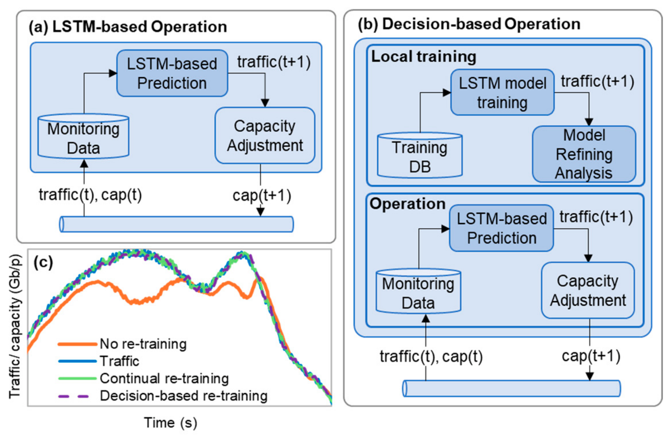Figure 1b shows the proposed architecture that addresses the limitations mentioned for the standalone model depicted in Figure 1a. Initially, the pre-trained model is deployed without adjustments, operating effectively as long as traffic characteristics remain consistent with the training data. However, when substantial changes occur, such as alterations in traffic periodicity or unforeseen traffic dynamics, that the model was not initially trained on, the accuracy of the predictions decreases.

A solution to this problem would be to continuously update the model with each new traffic data sample(s). However, this continual re-training approach significantly increases computational costs, not because each training is heavy but because frequent retraining (e.g., with every new sample) leads to a high cumulative computational cost. The proposed method where a decision-based retraining strategy is used in a separated local re-training phase can address this issue. This method integrates the LSTM-based prediction model with a Model Drift Detection Algorithm (MDDA). Instead of re-training continuously at every data point, the model is retrained selectively only when the prediction error exceeds a predefined threshold. The MDDA operates in conjunction with the LSTM predictor by calculating prediction errors and assessing whether they exceed a predefined threshold α, as expressed in Equation (3), where $y\left(t\right)$ is actual value, $\widehat{y}\left(t\right)$ is traffic prediction, and t − j is the interval window size, models the prediction error as a Gaussian (normal) distribution centered around the mean square error. As a result, it returns the normal distribution of error characterized by a range of standard deviation α (error tolerance). Then if the observed error exceeds the acceptable range, it signals a possible drift in traffic patterns and triggers retraining of the model [7]. This integration enables the LSTM model to adapt to new traffic patterns efficiently without requiring continuous re-training for each available for every connection, consisting of traffic and capacity samples over time. This approach ensures a balance between prediction accuracy and the frequency of re-training.

As shown in the enclosed graph in Figure 1c, three operational strategies for capacity management are compared: no-retraining, continual re-training, and decision-based re-training. The no-retraining approach (orange line) shows significant deviations over time as it fails to adapt to changing traffic patterns. In contrast, continual re-training (blue line) continuously updates the model, closely matching actual traffic capacity but at a high computational cost due to frequent re-training. In this approach, the model is updated for each data sample, ensuring per-sample accuracy. The decision-based re-training (purple dashed line) selectively updates the model based on specific criteria, balancing accuracy and computational efficiency. This method tracks traffic conditions as effectively as continual re-training, highlighting its advantage in adapting to dynamic environments.

The re-training approach introduced in our earlier work [7] was designed to adopt models for individual traffic flows. It relied on reactive updates triggered by drift detection to maintain accuracy. However, this method required re-training for each new flow, either partially or completely, making it difficult to scale across multiple traffic patterns. As a result, its performance was limited when applied to entirely new scenarios, especially those where no historical traffic data is available. To overcome these limitations, we introduce a cognitive transfer framework based on knowledge consolidation.

Instead of building and updating isolated models for each flow, we first construct a generalized model by consolidating multiple local models (from different scenario), each trained on different traffic profiles. This model consolidation, which is performed offline prior to the arrival of new flows, can serve as reusable knowledge. It is important to note that this consolidation is not a passive merging of models but involves a selective knowledge integration mechanism, where relevant knowledge from local models is combined to form an accurate general model. However, the core contribution of this work lies in how we selectively transfer knowledge from that general model to construct a new local model which is designed to arrival traffic flows or update the existing model particularly in zero-shot scenarios where training data is not available. This is achieved through a segment analysis process, where model components are scored based on relevance to the traffic flow, and only the most relevant segment is transferred. This selective transfer provides a lightweight initialization of the local model and avoids the inefficiencies of transferring or retraining the entire model.

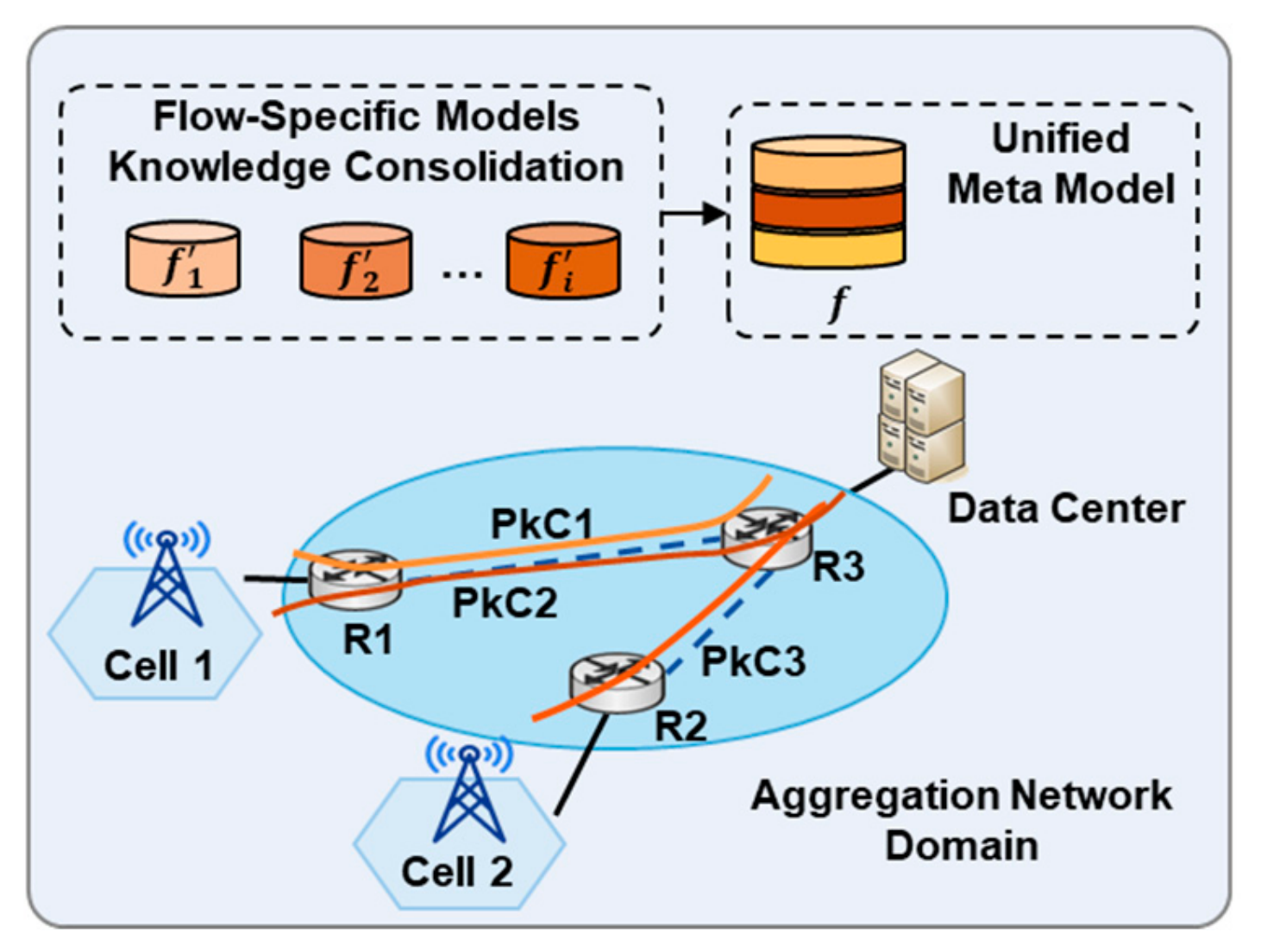
As an example, consider a scenario where a new connection is established from cell tower to the metro data center for a drone application. In the absence of prior data, the proposed approach (as illustrated in Figure 1) may fail in prediction, as the model is trained specifically for different traffic patterns. To cover this limitation, the approach proposed in this paper enables proactive adaptation by using a general model that is built in advance. This general model is created by consolidating several local models, each trained in different types of traffic patterns. As a result, it captures a wide range of behaviors and acts as a shared knowledge-base to be used when a new traffic flow appears. Then, our method selects the most relevant part of this general model that matches the characteristics of the new flow. These selected segments are then used to initialize a new local model or transfer in the existing model. This makes the local model perform almost as well as if it had been trained on local data, even though such data is not available at the time. This approach facilities proactive adaptation and lead to better capacity resources management. The proposed algorithm in this work avoids unnecessary model updates and lowers the overall computational cost compared to traditional methods. This makes the approach suitable for deployment in resource-constrained, low-latency environments, such as the network edge. The notation used throughout the paper is summarized in

Table 1. Notation.

Model and Learning Parameters
Symbol	Description
$G=(N,V)$	A graph G consisting of a set of nodes N and a set of edges $V.$
$f_i^{\prime }$	Local model trained on traffic flow $i.$
$f$	General (meta) model (e.g., LSTM-based) trained in historical data.
$\{f_1,\dots ,f_k\}$	Set of model subsets (segments) extracted from the meta-model $f.$
$f_k$(.)	$kth$ model segment (sub-model) extracted from the general model $f.$
$\{{\theta }_{k,1},\dots ,{\theta }_{k,m}\}$	Parameter subset associated with segment $f_k.$
${\overline{\theta }}_k$	Temporally smoothed or averaged parameter output for segment $f_k.$
$S_k$	Score assigned to segment $f_k$ based on correlation with input data.
$\{{\theta }_1\dots {\theta }_k\}$	Set of model substructures or segments used for evaluation and selection.
${\theta }^{\ast }$	Selected parameter subset corresponding to the highest scoring segment.
$f^{\ast }$	Selected optimal model or model substructure for knowledge transfer.
$Segment\left(f\right)$	Operation that decomposes model $f$ into identifiable substructures.
$\mathsf{\Psi }(.)$	Knowledge-aggregation function used in model consolidation.
$\rho (.,.)$	Pearson correlation coefficient function.
Traffic and Operational Parameters
Symbol	Description
$y\left(t\right)$	Ground truth (actual traffic volume or label) at time step $t.$
$\widehat{y}(t+1)$	Predicted traffic value at next time step $t+1.$
$x\left(t\right)$	Input vector for ONE time step $t$
$x_{1:n_k}$	Subset of input time series aligned in size with ${\mathsf{\Theta }}_k$ or $f_k.$
$\epsilon$	Prediction error $\widehat{y}(t+1)-y\left(t\right).$
$\epsilon .bound\left[\right]$	Statistically computed bounds (e.g., percentiles) used to determine model drift.
$\omega$	Window size for temporal smoothing in evaluation.
$\alpha$	Error-tolerance or confidence factor in drift detection.
$∆t$	Predefined batch size or window length used to calculate error thresholds.
$j$	Current index or iteration during real-time model execution.
$D$	Dataset (can be full training set or real-time monitoring data).
Mreply	Maximum replay-buffer capacity (number of most recent samples retained)

.

4. Cognitive Transfer Mechanism

The purpose of the proposed knowledge transfer mechanism is to enable an approach for network traffic prediction efficiently and accurately across many different flows or network scenarios, without needing to train a separate model from scratch for each one, particularly when local training data is limited or unavailable. Instead of training a new model for each flow, we use a consolidated general model built from previously trained models. Only the most relevant components of this general model are reused through a selective segment analysis process to enable a lightweight and accurate model initialization and adaptation.

We first detail the concept of knowledge consolidation to create a unified model by merging insights from individual models trained on specific traffic flows similar to the approach in [32]. Figure 2 illustrates the high-level deployment in a multi path scenario, where traffic flows originate from different access points (e.g., gNB 1 and gNB 2) and traverse multiple network segments (e.g., packet connection 1, 2, or 3) before reaching the data center. For each traffic flow, an individual predictive model $f_i^{\prime }$ is trained. These flow-specific models are then consolidated into a unified meta-model f, which captures generalizable traffic behavior across flows. To generalize the predictive capability across flows, we employ a knowledge-level consolidation strategy (see Figure 3, Model Consolidation) formalized in Equation (2). In particular, consolidation aggregates predictive behaviors at the output level via the operator $\mathit{\Psi } (.)$. This process is inspired by the aggregation concept in [32]. In our setting, consolidation is implemented as output-level aggregation; i.e., we combine the predictions of the individual models (rather than their internal parameters), which is consistent with ensemble learning.

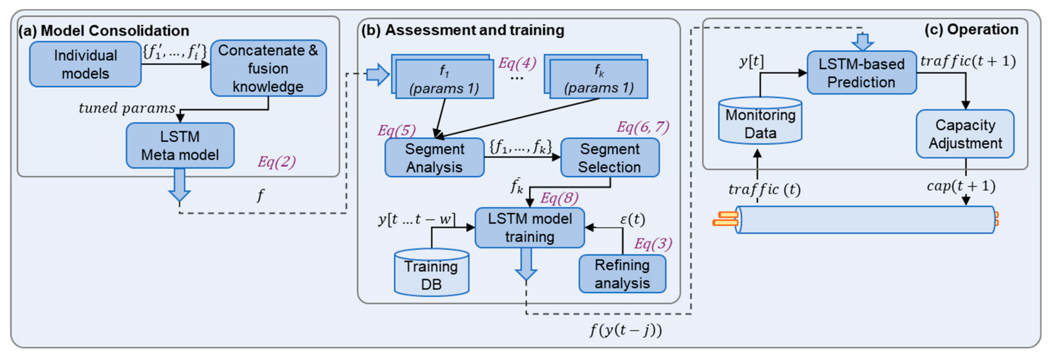
Now that we have a general understanding of what constitutes a good model, Figure 3 expands upon the consolidation pipeline by introducing the core components of the proposed framework.

As shown in Figure 3, the architecture consists of three phases: (a) Model Consolidation, (b) Assessment and training, and (c) Operation. Within these phases, the architecture comprises some functional modules: (i) Model Consolidation (phase a), (ii) Segment Analysis (phase b), (iii) Segment Selection (phase b), and (iv) Adaptive Retraining (phase b). In the Model Consolidation stage, previously trained flow-specific models $f_i^{\prime }$ are combined to form a unified meta-model. This consolidated model captures general behaviors observed across flows and serves as the shared knowledge base for subsequent adaptation. Instead of training a separate model for each new flow, the system reuses this shared knowledge to speed up deployment and reduce computational overhead. The inset in Figure 3b shows an example segmentation of a stacked LSTM, where each segment $f_k$ denotes an architectural block (subset of parameters), not a partition of time steps.

The Segment Analysis module examines the internal structure of the consolidated meta-model. The model is decomposed into several functional segments, each representing a coherent structural or temporal component of the original LSTM architecture. These segments are evaluated individually to understand how well each one aligns with the characteristics of the new traffic scenario. To ensure stable evaluation, the response of each segment is smoothed over a short time window, which filters out noise and preserves only the consistent behavioral patterns of each component.

In the Segment Selection module, the system determines which segment of the meta-model is most relevant for initializing the predictive model of the new flow. Each segment is assigned a score based on how closely its behavior matches the current traffic pattern. The segment with the strongest alignment is then chosen, ensuring that only the most useful part of the consolidated knowledge is transferred. This selective strategy prevents negative transfer and significantly reduces the size of the model portion that needs to be adapted.

The selected segment is then passed to the Adaptive Retraining module. This transfer is performed at the parameter level without changing the network topology or layer interfaces. In the stateless LSTM setting, hidden and cell states are recomputed from the input window after replacement, and the initialized model is then fine-tuned normally with gradients propagating through the transferred block. Here, a new LSTM-based predictive model is initialized using the knowledge transferred from the chosen segment. The model is further fine-tuned on the most recent traffic observations to adapt to any specific trends or short-term fluctuations. Retraining is performed only, when necessary, based on monitoring the prediction error over time. If the model’s performance deviates beyond statistically acceptable limits, a new refinement step is triggered; otherwise, the current model continues to operate unchanged. This on-demand retraining mechanism ensures that the system remains responsive to evolving traffic patterns while minimizing computational cost.

Once refinement is complete, the updated local model replaces the operational model and is used for forecasting upcoming traffic. Based on these predictions, the system can adjust network capacity proactively, reducing the risks associated with both under-provisioning and unnecessary over-allocation. By combining knowledge consolidation, selective reuse, and adaptive retraining, the framework achieves efficient and scalable predictive performance across diverse network environments.

4.1. Model Segmentation and Selection for Cognitive Transfer

The cognitive transfer mechanism operates by decomposing the consolidated meta-model into interpretable internal components and selecting the most relevant subset for adaptation to a newly observed traffic flow. This process begins by constructing a temporal representation of the current traffic behavior, defined as $x\left(t\right)$ in Equation (1), which captures the most recent sequence of traffic values over a window of size w. Prior to segmentation, the meta-model itself is formed through knowledge aggregation from previously trained local models. As expressed in Equation (2), the meta-model is obtained using the operator $\mathit{\Psi }(\cdot )$, which fuses the predictive behaviors of individual models rather than their internal parameters. This design preserves the functional diversity learned across different traffic scenarios and produces a unified predictive model that embodies a generalized representation of network dynamics.

$$f\left(x_t\right)=\mathsf{\Psi }(f_1^{\prime }\left(x_t\right), \dots , f_i^{\prime }\left(x_t\right))$$

(2)

$$\begin{gathered} gssMSE ~ \phi \left(mse\right(y\left(t-j\right),\widehat{y}(t-j)),{\alpha }^2) \\ j=0\dots t-1 \end{gathered}$$

(3)

After constructing the meta-model, the next step is to identify which internal components are most suitable for transfer to an unseen traffic flow. For this purpose, the meta-model $f$ is decomposed into a set of segments $\{f_1,f_2,\dots ,f_K\}$, each representing a coherent subset of the network corresponding to a distinct temporal or structural learning unit. Every segment is internally defined by its parameter subset $\{{\theta }_{k,1},\dots ,{\theta }_{k,m}\}$ (Equation (4)), which encapsulates the learned representations within that segment. Here, $m$ denotes the number of parameter groups in segment $f_k$.

Each ${\theta }_k$ corresponds to a coherent substructure of LSTM architecture. This might be reflecting a functional unit such as a temporal block, but non-trainable and stateless operations are excluded from this decomposition. Since the parameters of a segment may exhibit noise or short-term fluctuations, each segment is evaluated over a smoothing window. Equation (5) defines the smoothed representation where ${\theta }_{k,i}$ represents the response of the $k$-th segment within the $i$-th step of the evaluation window. This ensures that the representation of segment is smooth and segment evaluation does not overly depend on transient variations. Once the segmentation is defined, it remains fixed throughout all experiments.

$$\begin{gathered} \{ {\theta }_{k,j}{\}}_{j=1}^m\subset Segment\left(f_k\right) \\ k\in \left\{1,\dots ,K\right\}, m\in \mathbb{N} \end{gathered}$$

(4)

$${\overline{\theta }}_k={\displaystyle \raisebox{1ex}{$1$}\!\left/ \!\raisebox{-1ex}{$w$}\right.}\sum _{i=1}^w{\theta }_{k,i}$$

(5)

Each smoothed segment is then evaluated through a correlation-based scoring function. The relevance score $S_k$ in Equation (6) is computed between the smoothed representation and the corresponding slice of the input window $x_{1:n_k}$, aligned to match the dimensionality of the segment. Pearson correlation [33] is used to measure how closely the segment behaves relative to the observed traffic pattern.

The Pearson correlation is selected because it is computationally inexpensive and scale-invariant, making it well-suited for time-critical selection decisions. However, the framework is not tied to this choice: the same scoring interface can incorporate alternative relevance measures such as Spearman rank correlation [34] or distance-based measures [35].

Segments whose smoothed outputs are more consistent with the local traffic window receive higher scores. The best segment is then selected using Equation (7), where ${\theta }^{\star }$ identifies the substructure that exhibits the strongest match with the input data. This selected subset forms the basis of the transferred model. The resulting model is denoted by $f^{\star }$ in Equation (8), which initializes a new LSTM configuration using only the selected segment rather than the full meta-model. This reduces transfer cost and avoids unnecessary parameter adaptation. Once initialized, the model undergoes refinement through the adaptive re-training mechanism described earlier. Retraining is triggered only when errors exceed the statistically defined bounds derived from Equation (3), which is parameterized by $\alpha$ as the standard-deviation-based error tolerance and adjusted by $\theta$ to enlarge the analyzed range. Therefore, retraining occurs only when the MSE-based error falls outside the expected Gaussian error bounds, suggesting model drift and reduced prediction reliability. This selective update process ensures that the transferred model adapts to deviations in the traffic without requiring continuous or full-model retraining.

$$S_k=\rho \left({\overline{\theta }}_k{x}_{1:n_k}\right)$$

(6)

$${\theta }^{\ast }={arg}_{k\in \{1\dots ,K\}}max{S}_k$$

(7)

$$f^{\ast }\left(.\right)=(.;{\theta }^{\ast })$$

(8)

As an example, let us consider a predictor with architecture $f\left(x\right)=Dens{e}_2\left(ReLU\right(Dens{e}_1\left(LST{M}_2\right(LST{M}_1\left(x\right)\left)\right)\left)\right)$. In the proposed framework, a segment is defined as an interface-compatible trainable block of the predictor. Accordingly, one possible segmentation can be $Segment\left(f\right)=\{f_1,f_2,f_3\}$, where $\left\{{\theta }_{\mathrm{1,1}},\dots ,{\theta }_{1,m}\right\}$ belongs to $f_1$, $\left\{{\theta }_{\mathrm{2,1}},\dots ,{\theta }_{2,m}\right\}$ belongs to $f_2$, $\left\{{\theta }_{\mathrm{3,1}},\dots ,{\theta }_{3,m}\right\}$ belongs to $f_3$. For a newly observed traffic flow, these segments are evaluated over the target window and smoothed, resulting ${\overline{\theta }}_1$, ${\overline{\theta }}_2$, and ${\overline{\theta }}_3$. These smoothed representations are then compared with the aligned target-flow input using the Pearson-based score, producing scores $S_1$, $S_2$, and $S_3$. If, for instance, $S_2$ is the largest, then selects ${\theta }^{\ast }={\theta }_2$. This selected subset is used to initialize the corresponding block of the target model, resulting in $f^{\ast }(\cdot ;{\theta }^{\ast })$. The initialized model is then refined on the available samples of the new flow.

4.2. Adaptive Re-Training Mechanism for Model Enhancement

To complement the architectural description presented earlier, this subsection formalizes the workflow of the proposed cognitive transfer framework from an algorithmic perspective. The consolidation, segment analysis, and segment selection procedures have already been described conceptually in the previous sections and are summarized in Algorithms 1 and 2. These steps provide the meta-model, the relevance evaluation of its internal segments, and the initialization of a new local model using the most appropriate segment for the arriving traffic flow. Once the local model is initialized, the framework transitions into the operational phase, where the main objective is to maintain accurate predictions while minimizing retraining overhead. M_reply is the maximum number of recent samples kept in memory, and the buffer is that memory itself. The buffer is first filled with the most recent samples from the initial data up to size M_replay, and later, when the prediction error goes outside the accepted bounds, the model retrains using the buffered past samples together with the new sample so it can adapt without full retraining every time. This phase is governed by the dynamic model refinement mechanism, formally described in Algorithms 1–3.

Algorithm 1: Segment Analysis and Scoring
INPUT: meta-model f, Ytarget, w, ω, K OUTPUT: segments fk, scores Sk
1:   2:   3:   4:   5:   6:   7:   8:	decompose f into K segments {f1, …, fK} for each segment fk do   evaluate segment outputs over Ytarget using window length w   smooth segment outputs using a temporal window of size ω   align smoothed outputs with corresponding target values   compute correlation-based score Sk end return fk, and Sk

Algorithm 2: Segment Selection and Model Initialization
INPUT: meta-model f, segments fk, scores Sk, Dinit, Mreplay OUTPUT: initialized model, buffer
1:   2:   3:   4:   5:   6:   7:   8:	k* ← index of maximum score in Sk extract parameters of segment fk* initialize new local model using selected parameters if Dinit is not empty then   perform short warm-up training on Dinit end construct buffer using most recent samples from Dinit up to size Mreplay return model and buffer

Algorithm 3: Dynamic Model Refinement
INPUT: model, buffer, streaming data (yt), batch size Δt OUTPUT: updated model
1:   2:   3:   4:   5:   6:   7:   8:   9:  10:  11:  12:  13:  14:  15:  16:  17:  18:  19:	initialize error-list ← ∅ j ← 0 while j < Δt do   predict ŷt ← model.predict(y{t − w + 1:t})   error_list.append(ŷt − yt)   j ← j + 1 end lower-bound, upper-bound ← percentile(error_list) while TRUE do   predict ŷt ← model.predict(x{t − w + 1:t})   ε ← ŷt+1 − yt   if ε < lower-bound or ε > upper-bound then     training-batch ← buffer ∪ {(x{t − w + 1:t}, yt)}     model.fit(training-batch)     update(buffer, (x{t − w + 1:t}, yt))   end   t ← t + 1 end while return model

In this refinement stage, the model no longer performs full-scale retraining but instead adapts selectively based on real-time performance. The process begins with a warm-up phase, where the model collects an initial set of prediction errors over a fixed batch of incoming samples. These errors are used to compute statistical error bounds that represent the normal operating behavior of the model under stable conditions. Unlike static thresholds, these bounds are derived from empirical percentiles of the observed errors, allowing the system to adjust naturally to the inherent variability of each traffic environment.

4.3. Scenarios

To illustrate the application of the cognitive transfer mechanism and its architecture discussed in the previous sections, we present two representative scenarios.

4.3.1. Transport Communication Scenario

This scenario involves adaptive traffic prediction in public transport communication networks, where virtual network links are dynamically established to accommodate varying traffic demands. Accurate traffic prediction for these links is essential for optimal resource allocation, congestion prevention, and maintaining high-quality service. The knowledge transfer-based operation supports efficient model selection and refinement in this context.

Each virtual link employs an LSTM-based model to predict future traffic loads using real-time monitoring data, such as packet flow, latency, and link utilization. When the network’s central management system detects significant traffic pattern changes not captured by the current model, it initiates a knowledge assessment process. This process selects a new model or refines the existing one using knowledge transferred from other virtual links with similar traffic patterns. This adaptive approach enables the central management system to dynamically select the most suitable predictive model for each virtual link, ensuring optimal bandwidth utilization and minimizing disruptions. By transferring knowledge across virtual links and reducing reliance on frequent full-scale re-training, the network remains agile and responsive to fluctuating traffic demands.

4.3.2. Smart Grid Scenario

This scenario focuses on smart grids, where energy demand is highly variable due to factors such as weather conditions, time of day, and consumer behavior. Effective management of these dynamics is critical for grid stability and efficiency [36]. Transfer learning has proven to be an effective method for addressing challenges like data scarcity and the computational complexity of training machine learning models from scratch in energy systems. Each sector of the grid system employes a LSTM model trained on sector specific data, such as residential buildings, industrial facilities, or renewable energy sources (e.g., solar or wind farms). By integrating these sector-specific models into a generalized ensemble model, the system captures diverse patterns, enabling more accurate and adaptive forecasting in underrepresented or new sectors. This ensemble model provides a robust mechanism for knowledge transfer across sectors, allowing efficient prediction and resource management even in scenarios with limited local training data.

5. Results

This section presents simulation results to validate the proposed module described in previous section. In this study, we utilized the Abilene network topology and its associated traffic dataset to create a simulation environment for evaluating network performance. Since the evaluation focuses on transport-level traffic prediction (metro/backhaul), rather than RAN-level dynamics, the Abilene dataset is a suitable benchmark for this work. The Abilene network topology is composed of a series of interconnected nodes (routers), which represent major geographic locations across the United States.

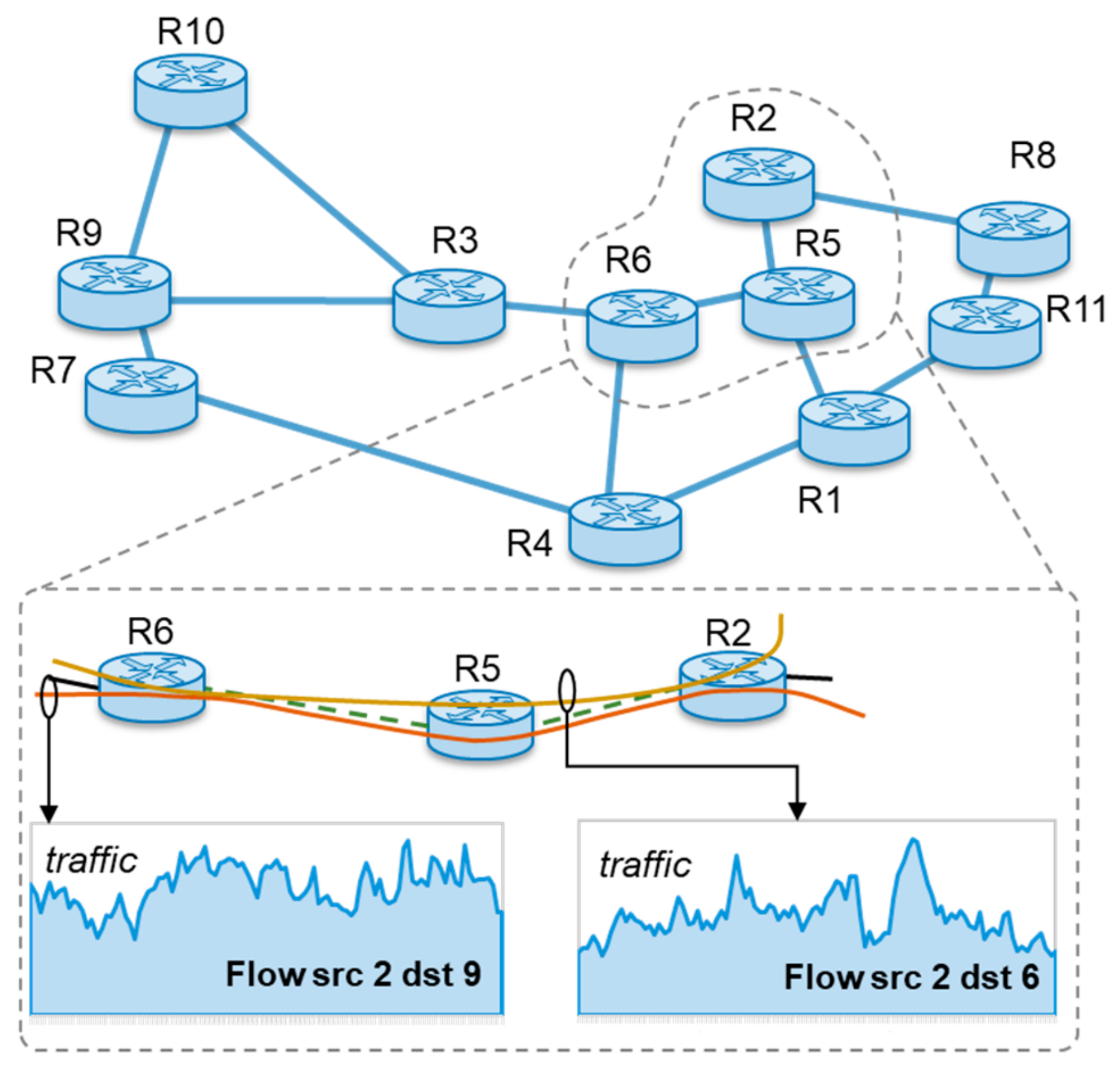
These nodes are linked to form the backbone of Internet2, as depicted in Figure 4. This topology provides a realistic model of large-scale network operations, making it an ideal choice for simulation. By replicating the physical layout and connection patterns of the Abilene network, we were able to closely simulate real-world traffic flow and network behavior based on reference [37,38]. Abilene dataset provides detailed metrics, such as traffic volume and packet count between nodes, offering a rich source of information for analysis. Using reference topology, various scenarios were created by selecting origin destination node pairs within the network. For each scenario, the aggregated traffic was dimensioned to match the sum of flows traversing all paths, measured in 5 min intervals (see Figure 4 for an example).

The dataset is organized as a time-series of traffic matrices representing inter-node volumes across the Abilene network. Each traffic matrix captures the network state at a 5 min interval, with entries corresponding to the volume of traffic between all pairs of the 11 backbone nodes. The data is hierarchically organized by month and day, covering the period from March to mid-September. For each day, a sequence of 288 matrices (one per 5 min interval over 24 h) is available, which provides data for predictive analysis. These matrices form the basis for constructing input time series for our model.

To derive the input for each Origin–Destination (O-D) scenario, we first compute all shortest paths across the Abilene topology using NetworkX [39]. Then, for a selected O-D pair, we extract the traffic corresponding to the endpoints of all such paths that traverse both nodes. The aggregated traffic at a given time is calculated by summing the volumes along these paths from the respective traffic matrices. This process is repeated across the dataset to build a complete time series of aggregated traffic for the selected node pair.

All simulations and model evaluations were executed on a virtual machine in EXTREME Testbed^® at the Centre Tecnològic de Telecomunicacions de Catalunya (CTTC), Castelldefels, Barcelona, Spain, accessed remotely via SSH. The VM configuration provides 16 CPU cores, 64 GB RAM, and 400 GB of disk storage. The experimental workflow was implemented in Python 3.9. The data preprocessing and traffic aggregation pipeline were developed using NumPy 1.26 and Pandas 1.5.3, while shortest-path computation over the Abilene topology was performed using NetworkX 3.5. The LSTM models were implemented using TensorFlow 2.20 and Keras 3.11.

To validate the accuracy of the proposed methodology for predicting the aggregated traffic on a given link, we performed an analysis assuming the availability of an accurate general ensemble model. For this purpose, a dataset consisting of 48,000 samples was selected from a specific link along the path between node 2 and node 6. To preserve the temporal integrity of the time-series, we performed a sequential data split: the first 50% of the samples were used for training, and the remaining 50% were used for validation. No random shuffling was applied, ensuring that the model was trained strictly on past data and validated on future data in chronological order. Note that this split is used only for training and validation within a given traffic flow and does not define the mapping between a flow type and the selected transferable segment. This mapping is determined separately by scoring candidate segments against the target flow using Equations (6) and (7).

The prediction model employed was an LSTM network comprising four sequential layers with 10, 20, 10, and 5 units, respectively. The training process was conducted over 20 epochs with a batch size of 100. While initial evaluations focused on a representative path between node 2 and node 6 to illustrate the methodology, the simulation study was later extended to multiple origin–destination pairs across the Abilene topology (e.g., nodes 1–8, 6–10, 3–7, and 4–6, as shown in Figure 5). Each scenario was evaluated independently, using its own time-series data and model training. This allowed us to validate the consistency of the proposed method under varying traffic dynamics. Although random sampling in simulations was not performed, the repeated testing over distinct network paths and traffic conditions serves a comparable purpose in demonstrating robustness and generality of the results.

5.1. Effectiveness of the Cognitive Model Selection Strategy

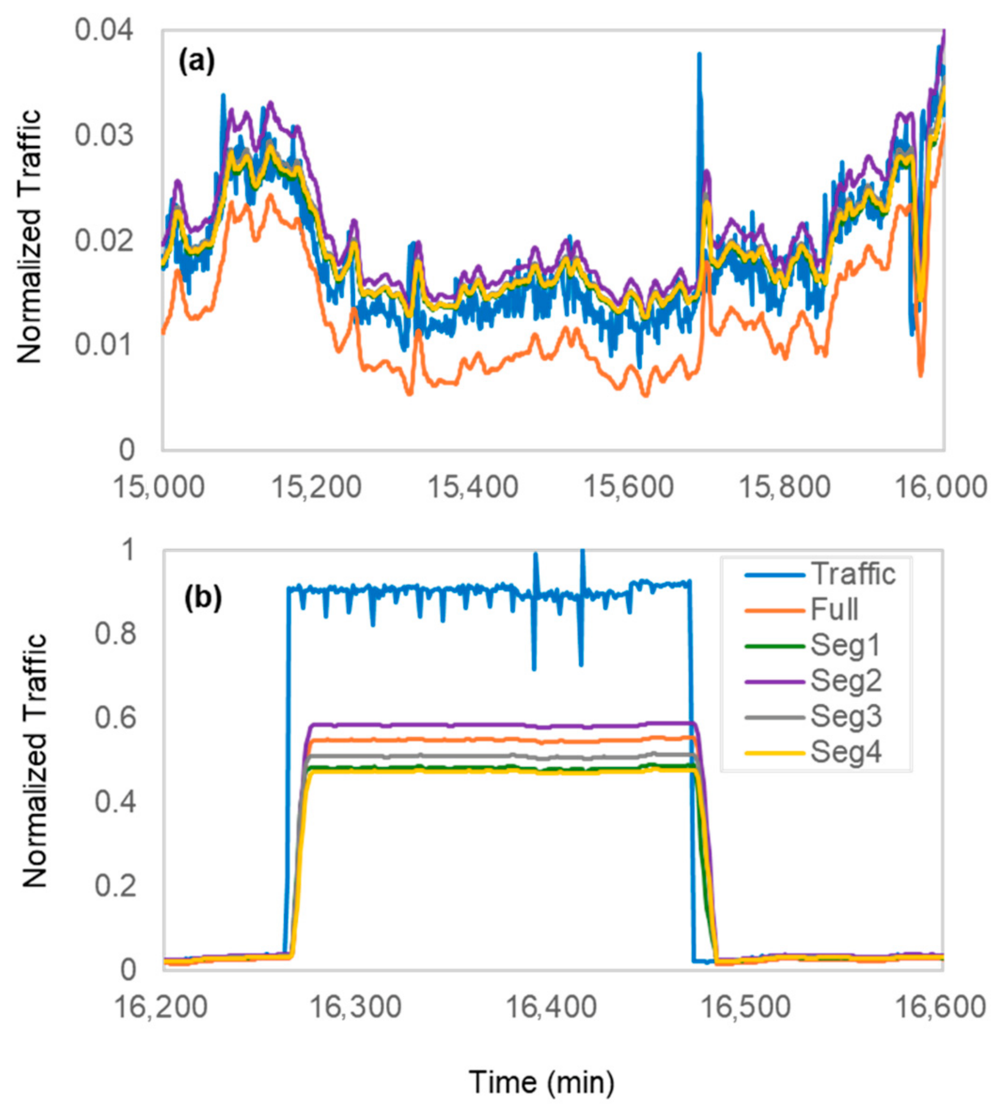
Figure 5 shows the normalized prediction error (scaled between the minimum and maximum values) over time for two representative traffic scenarios, under five distinct model architectural conditions. These conditions include the full model transfer and partial model transfer to the specific layers of the model as it is depicted in the figure. The prediction error has been normalized between its minimum and maximum values to emphasize relative trends. Each test was conducted independently to ensure that segment(s) transfer was applied to a newly initialized model. This means the transferred segment remained fixed during the evaluation period; the figure does not reflect dynamic or real-time switching between segments.

Figure 5a presents a traffic scenario with smoother and more stable volume patterns, making it relatively easier to predict. In contrast, Figure 5b depicts a highly volatile traffic pattern characterized by sharp peaks and irregular fluctuations representing a more challenging scenario where achieving accurate predictions is significantly more difficult. In both scenarios, all prediction methods tend to underestimate the actual traffic to some degree, particularly during sudden spikes.

Although all prediction methods underestimate traffic during sharp peaks, as seen in Figure 5b, Segment 2 consistently reduces the gap between predicted and actual demand. While this does not eliminate the risk of under-provisioning, it significantly reduces its severity and frequency. By providing more accurate forecasts, Segment 2 improves the reliability of bandwidth estimation, which can enhance decision-making in systems that depend on traffic prediction for resource allocation.

Table 2. Prediction Error.

Approach	High Var	Low Var	MSE
Full	14%	15.2%	0.0021
Seg 1	75.42%	71.7%	0.0025
Seg 2	8.5%	7.9%	0.0018
Seg 3	10%	10%	0.0023
Seg 4	92.75%	59.1%	0.0026

presents the quantitative evaluation of the prediction performance across the same two traffic conditions shown in Figure 5: high-variability and low-variability flows. For each configuration (Full model and Segments 1–4), the table reports two key metrics: the percentage of under-prediction events and the Mean Squared Error (MSE).

High-variability traffic refers to scenarios with frequent and significant fluctuations in volume, whereas low-variability traffic is characterized by smoother, more predictable patterns.

An interesting observation from Table 2 is that Segment 2 occasionally outperforms the Full model in both the MSE and under-prediction rate. This may be because Segment 2 captures generalizable temporal patterns that align closely with the target traffic behavior. In contrast, the Full model, though more comprehensive, may include components that are overfitted to unrelated source traffic conditions, reducing its transfer effectiveness. This highlights the advantage of selective segment reuse, where a well-matched subcomponent can achieve better adaptability and accuracy than the entire model.

Among all configurations, Segment 2 achieves the lowest under-prediction rates in both traffic scenarios, as well as the lowest overall MSE value (0.0018). This confirms the visual trend observed in Figure 4, where Segment 2 closely tracked the actual traffic. The Full model transfer approach also performed well, with a slightly higher MSE (0.0021), making it a competitive, though less efficient alternative, possibly due to inclusion of components that are overfitted to unrelated source traffic conditions. Segment 3 provided moderate accuracy (MSE of 0.0023), while Segments 1 and 4 underperformed, particularly under high-variability conditions, with under-prediction rates of 75.42% and 92.75% respectively, and MSE values exceeding 0.0025.

These results highlight the importance of segment selection: some components of the model generalize better than others when transferred to a new traffic flow. Table 2 validates the effectiveness of the proposed segment scoring mechanism and supports the argument for selective reuse over full-model transfer.

5.2. Prediction Accuracy of Selected Models

5.2.1. Model Performance Analysis

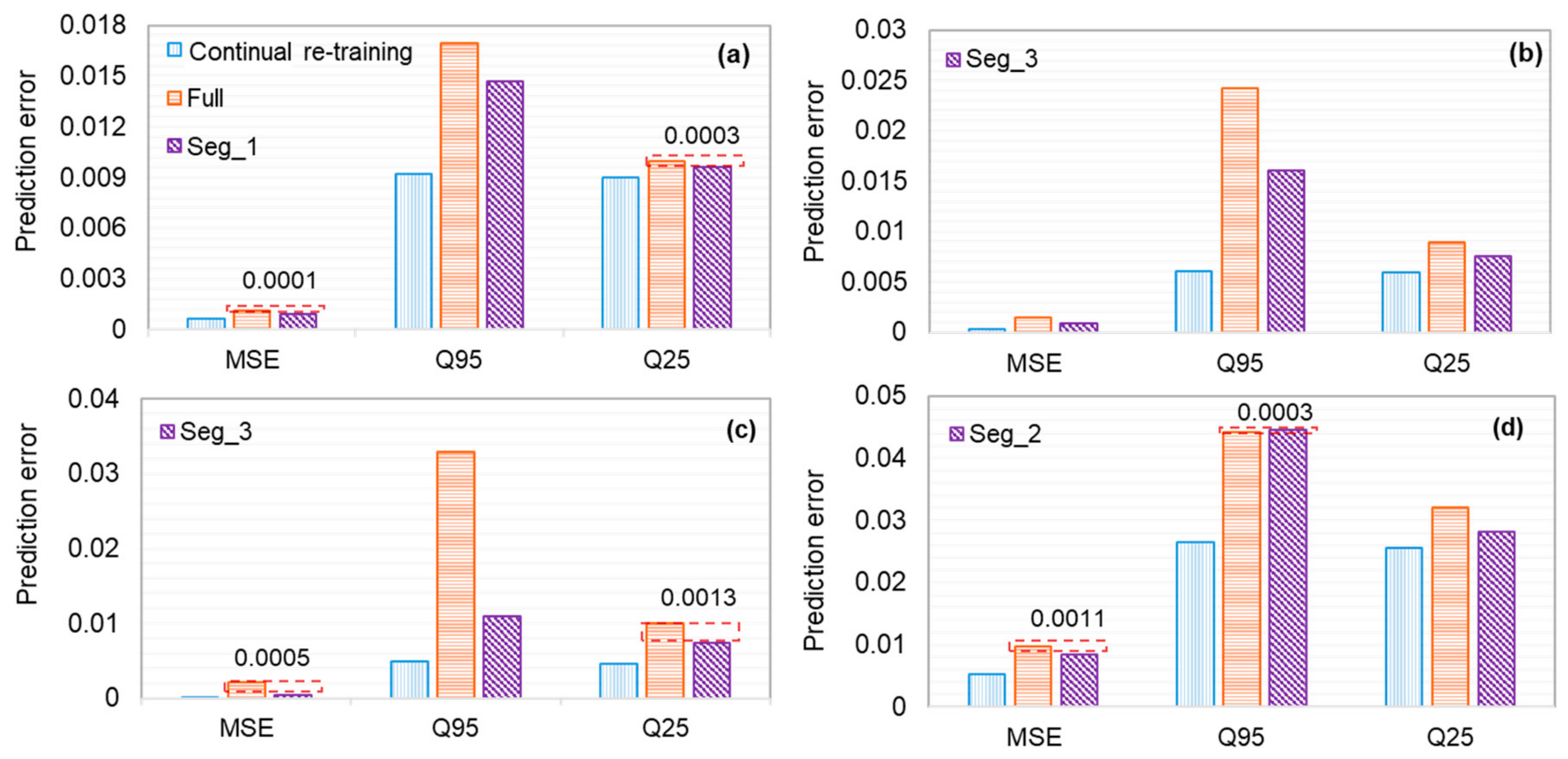
Figure 6 illustrates the performance of three approaches, continual re-training (blue), full model transfer (orange), and segment-based transfer (purple), across four network paths: Node 1 to 8, Node 6 to 10, Node 3 to 7 and Node 4 to 6. The dataset included aggregated traffic data over a 15-day period, with each day comprising 128 data points, resulting in a total of 1920 data points. For the continuous operation scenario, re-training was triggered for each data point, amounting to 1920 re-trainings in total.

This setup served as a baseline reference for assessing computational cost in a non-optimized system.

Performance was evaluated using key metrics: MSE, quantile error at 95% (Q-95), and quantile error at 25% (Q-25). These metrics were selected to measure both general prediction accuracy and the impact of asymmetric errors. Specifically, Q-95 emphasizes the consequences of under-prediction, which may lead to traffic loss, while Q-25 identifies over-prediction, which can result in inefficient resource allocation due to over-provisioning. As shown in Figure 6, the online learning approach consistently achieved the lowest prediction errors, confirming its expected precision. Both the full model transfer and segment-based transfer methods demonstrated similar performance in terms of MSE and Q-25, with only minor differences. However, for Q-95, which highlights under-prediction errors, the full model transfer approach exhibited higher error values across all paths compared to the segment-based transfer approach. This suggests a higher risk of packet loss in the full model transfer scenario. The only negligible exception was the path from Node 4 to Node 6, where the Q-95 error differed by just 0.0003.

In summary, the proposed method was validated under dynamic, time-varying traffic and multi-domain conditions. The results confirm the segment-based transfer approach provides superior prediction accuracy, particularly by reducing under-prediction errors while maintaining efficient resource utilization.

5.2.2. Comparison with State-of-the-Art Models

To evaluate the effectiveness of our proposed method, we compare its performance against several state-of-the-art models for network traffic prediction.

Table 3. Traffic Prediction Results or State-of-the-Art Approaches on the Abilene.

Model	Technique	MSE	RMSE	MAE
ViT GRU [40]	Vision Transformer + GRU	0.0308	0.1754	0.1338
ViT LSTM [40]	Vision Transformer + LSTM	0.0358	0.1891	0.1468
LTGG [41]	Layered Training GCN + GRU	0.0027	0.522	0.0200
GCN_LSTM [41]	Graph Convolutional Network + LSTM	00.34	0.0601	0.0211
Transfer-LB	LSTM + Selective Segment Transfer	0.0027	0.0434	0.0323
Transfer-HB	LSTM + Selective Segment Transfer	0.0023	0.0379	0.0283

presents a comparison of the MSE, Mean Absolute Error (MAE), and Root Mean Squared Error (RMSE), across five representative models from recent literature. These include GCN-based architectures (LTGG, GCN_LSTM) and transformer-enhanced models (ViT LSTM, ViT GRU).

The models represent two dominant directions in network traffic prediction: (i) graph-based spatio-temporal predictors, which exploit topology-driven spatial correlations, and (ii) transformer-enhanced predictors, which use attention mechanisms and often involve higher training costs. In contrast, our contribution is not a new backbone predictor but an efficient adaptation strategy that selectively transfers only relevant components and updates them on demand. Our proposed method evaluated under High Band (HB) and Low Band (LB) error conditions.

Concretely, HB corresponds to tighter percentile bounds (higher sensitivity) that trigger more frequent updates to maintain accuracy, whereas LB corresponds to wider bounds (lower sensitivity) that reduce update frequency to save computation. For fairness, the error values in both High Bound (HB) and Low Bound (LB) settings are averaged across the four OD flows shown in Figure 6. HB and LB are the two error threshold levels used by the decision-based retraining mechanism: HB uses a stricter (lower) tolerance band, which triggers more frequent model updates to maintain higher prediction accuracy, whereas LB uses a more relaxed (higher) tolerance band, reducing the update frequency to conserve computational resources.

As shown in Table 3, although the High Band approach achieves the lowest values in MSE and RMSE, its MAE is not the lowest among all models. This is practically important because prediction-based resource allocation is executed continuously; therefore, lower adaptation cost enables more frequent model refresh under the same compute budget. Operationally, maintaining similar RMSE and MAE with fewer updates reduces both (i) the risk of under-provisioning events caused by stale models and (ii) the compute overhead required to keep the predictor accurate in production.

This can also be explained by the model’s selective update strategy, which triggers retraining only when prediction errors exceed predefined thresholds. While this effectively prevents large errors (heavily impacting MSE and RMSE) it allows small to moderate errors within the tolerance band to persist, which contributes to a slightly higher MAE.

5.3. Training Cost Across Model Update

Table 4. Percentage Reduction in Re-training Frequency. Unshaded rows correspond to the LB setting, while gray-shaded rows correspond to the HB setting.

Approach	1 to 8	3 to 7	4 to 6	6 to 10
Full	61.61%	73.12%	20.72%	91.77%
	12.55%	47.18%	32.91%	56.56%
Segment	77.6%	89.27%	64.01%	92.29%
	12.91%	60.41%	16.77%	51.51%

extends the analysis beyond prediction error by considering additional metrics, such as computational cost, evaluated based on the number of re-trainings operations triggered by the algorithm. Our proposed approach was tested across four traffic paths, similar to the ones selected in previous sections and compares the segment-based and full model transfer approaches. We evaluated both approaches under two threshold levels: LB represented in white rows HB shown in gray rows in Table 4. Each cell in the table reports the percentage reduction in re-training, calculated relative to the total number of full model re-training iterations.

For the path from Node 1 to 8, the number of re-trainings under the LB condition was 737 for the full-transfer approach and 430 for the segment-based approach. Under the HB condition, these counts increased to 1679 and 1672, respectively. For the path from Node 6 to 10, the counts were 158 and 148 under LB, rising to 834 and 931 under HB. For the path from Node 3 to 7, the re-training counts were 516 and 206 under LB, and 1014 and 706 under HB. Finally, for the path from Node 4 to 6, the counts were 1522 and 691 under LB, compared to 1288 and 1598 under HB.

The results show that the segmented approach experiences a slight increase in re-training frequency under stricter threshold conditions (HB) compared to the full-transfer approach. This is due to the characteristics of partial model transfer, which make the model more sensitive to minor deviations, triggering more frequent adjustments. Occasionally, this increased sensitivity may lead to overfitting small variations. Despite these challenges, the segment-based approach offers significant advantages by focusing on selectively transferring and adapting only the most relevant model component. This avoids the resource-intensive process of re-training the entire model while maintaining comparable or even superior accuracy. Overall, this approach achieved a balanced trade-off by combining the benefits of targeted model transfer with the efficiency of reduced re-training, resulting in lower complexity and improved handling of network traffic. This is especially beneficial in scenarios where accurate prediction and minimal traffic loss are essential. The effectiveness of the segment-based method is further supported by the Q-95 and Q-25 metrics, which validate its ability to address under-prediction challenges. This makes the approach a robust and efficient solution for traffic prediction in the dynamic and evolving landscape of 5G and 6G networks.

6. Conclusions

This paper proposes a framework based on model consolidation, selective knowledge transfer and statistical techniques for dynamic resource allocation. The simulation results using the Abilene dataset demonstrate that the proposed approach enhances network performance by optimizing resource utilization, which leads to reduced latency and packet loss. The framework also proves computationally efficient, reducing model retraining frequency through statistical analysis techniques, achieving a maximum reduction of 43.29% with a flexible threshold, compared to the full approach and 13.23% with strict thresholds, while it maintains the prediction accuracy. It is worth noting that selective knowledge transfer minimizes the size of the transferred knowledge and simplifies building model by focusing on the most relevant components. Future work could explore the scalability and energy efficiency of the framework to support large-scale device deployments, as efficient resource management reduces energy consumption and ensures sustainable operation in large-scale networks.