Figure 1.
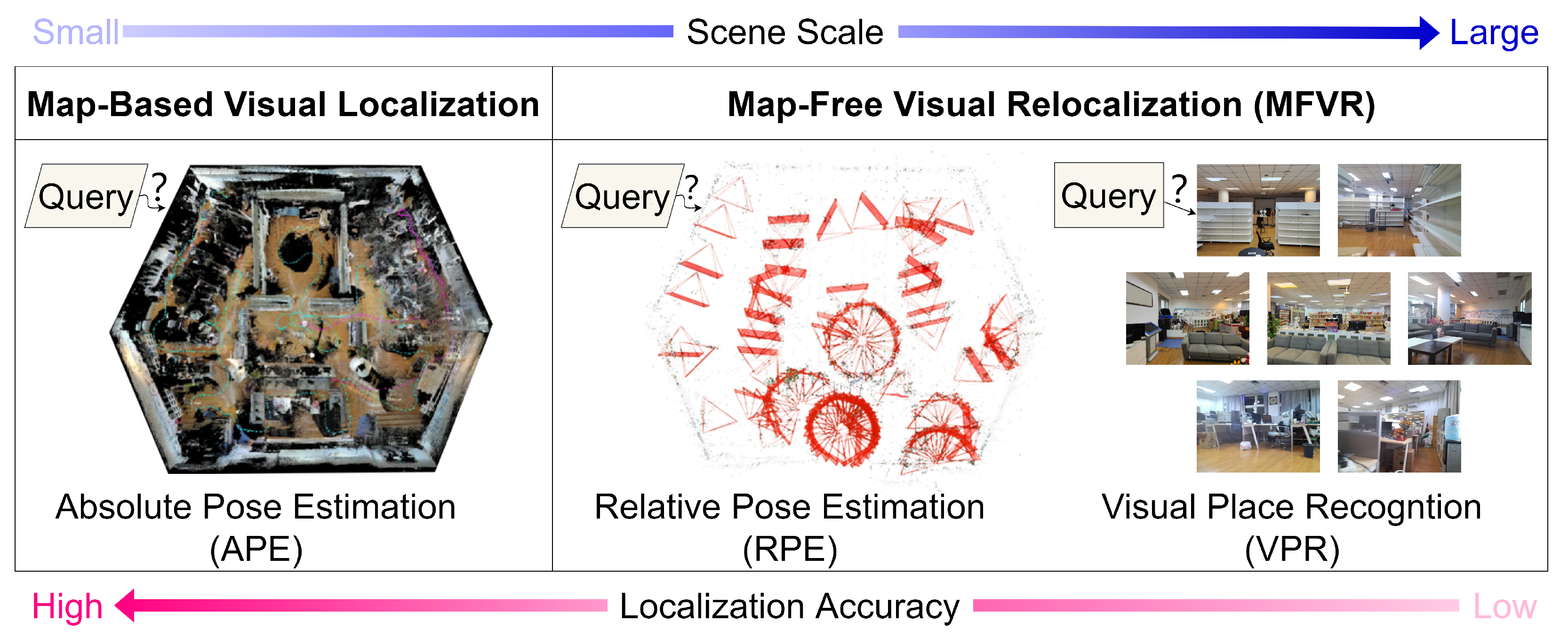
Main paradigms of visual localization. For a query image, absolute pose estimation (APE) matches it directly to the 3D scene map, while relative pose estimation (RPE) and visual place recognition (VPR) need to retrieve the reference dataset. Moreover, RPE is supposed to make a better trade-off between scene scale and position accuracy.
Figure 1.
Main paradigms of visual localization. For a query image, absolute pose estimation (APE) matches it directly to the 3D scene map, while relative pose estimation (RPE) and visual place recognition (VPR) need to retrieve the reference dataset. Moreover, RPE is supposed to make a better trade-off between scene scale and position accuracy.
Figure 2.
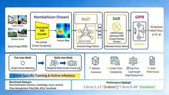
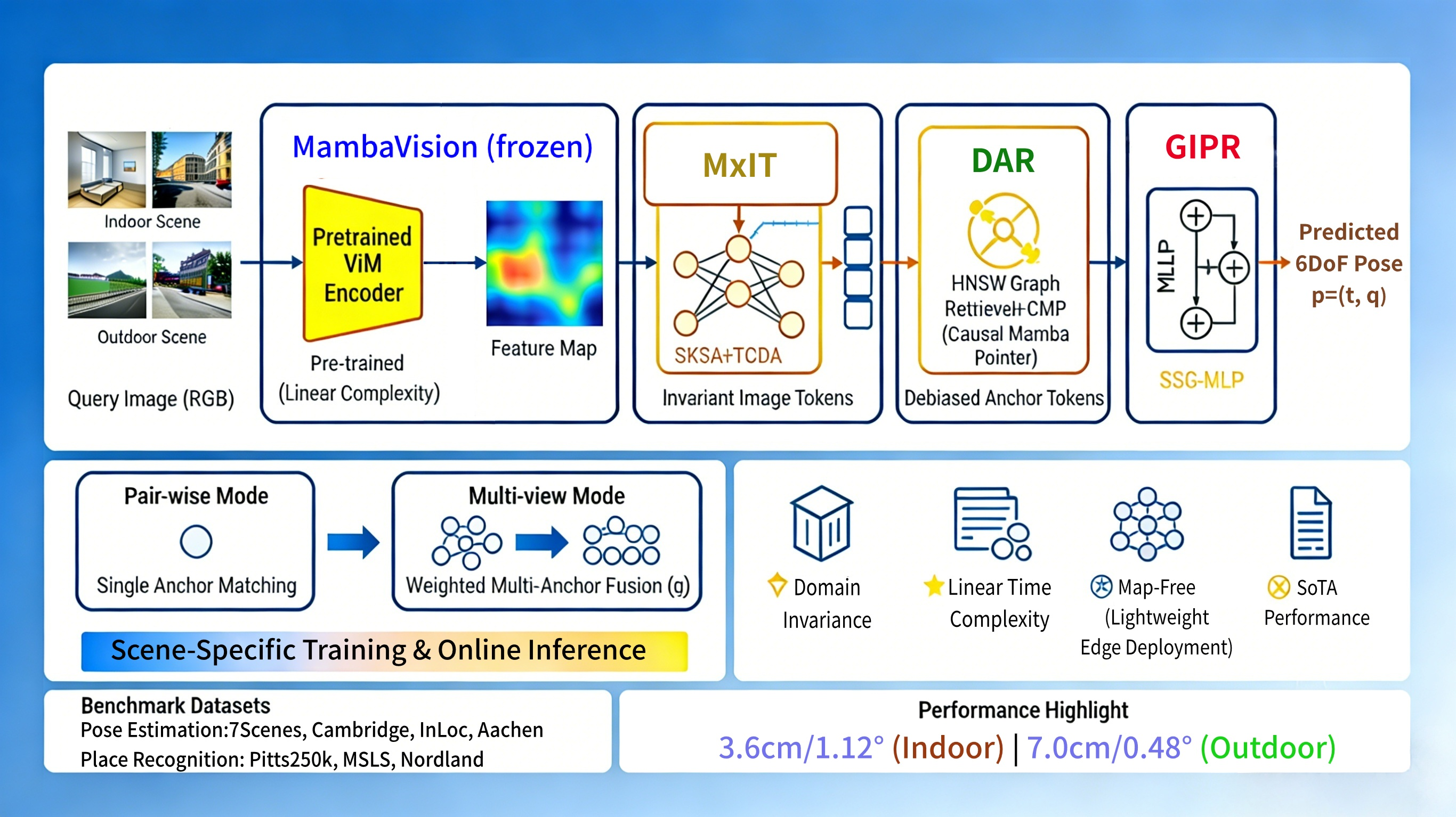
The pipeline of our proposed method. Four modules are designed and cascaded for relative pose regression (RPR): fronzen Pretrained ViM Encoder, Multiplex Interactive Tokenization (MxIT), Debiased Anchor Registration (DAR), and learnable Geometry-Informed Pose Regression (GIPR).
Figure 2.
The pipeline of our proposed method. Four modules are designed and cascaded for relative pose regression (RPR): fronzen Pretrained ViM Encoder, Multiplex Interactive Tokenization (MxIT), Debiased Anchor Registration (DAR), and learnable Geometry-Informed Pose Regression (GIPR).
Figure 3.
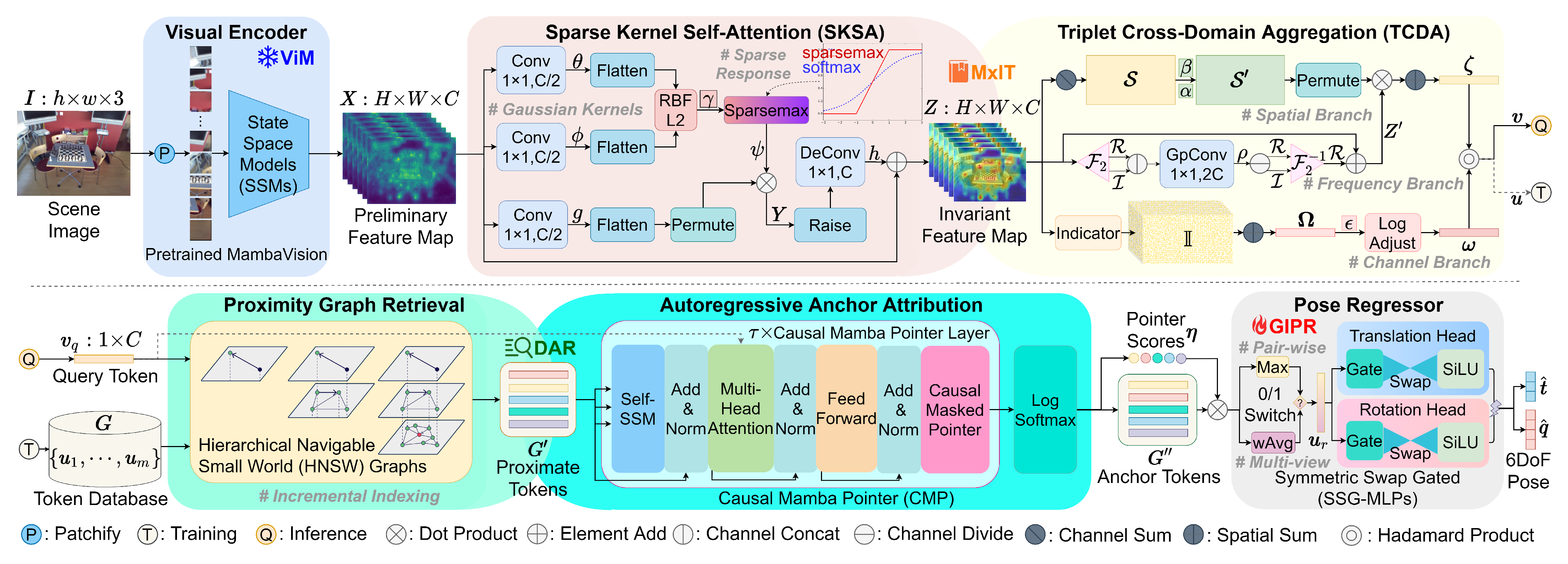
Overview of the DMT-Loc framework. It sequentially performs self-attentive mapping from images to tokens and causal attentive regressing to poses. RBF, DeConv, and GpConv stand for radial basis function, deconvolution, and grouped convolution, respectively.
Figure 3.
Overview of the DMT-Loc framework. It sequentially performs self-attentive mapping from images to tokens and causal attentive regressing to poses. RBF, DeConv, and GpConv stand for radial basis function, deconvolution, and grouped convolution, respectively.
Figure 4.
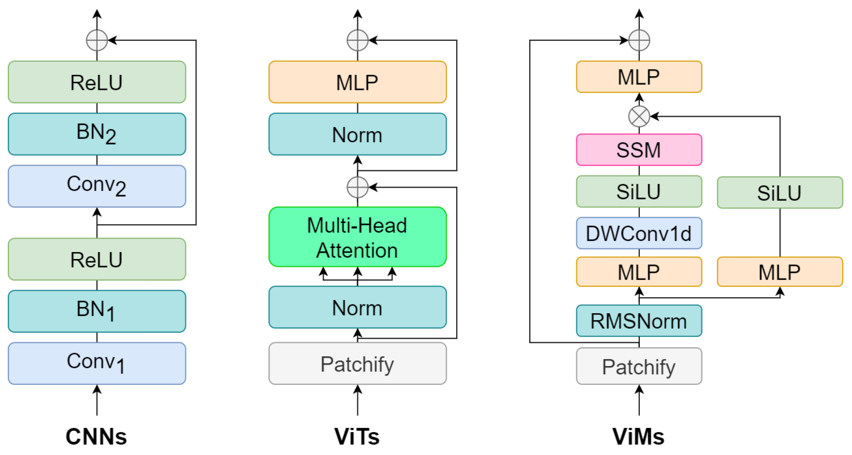
Structural comparison of CNN, ViT, and ViM. ViM offers the global receptive fields of ViT while maintaining linear computational complexity via state-space models (SSMs).
Figure 4.
Structural comparison of CNN, ViT, and ViM. ViM offers the global receptive fields of ViT while maintaining linear computational complexity via state-space models (SSMs).
Figure 5.
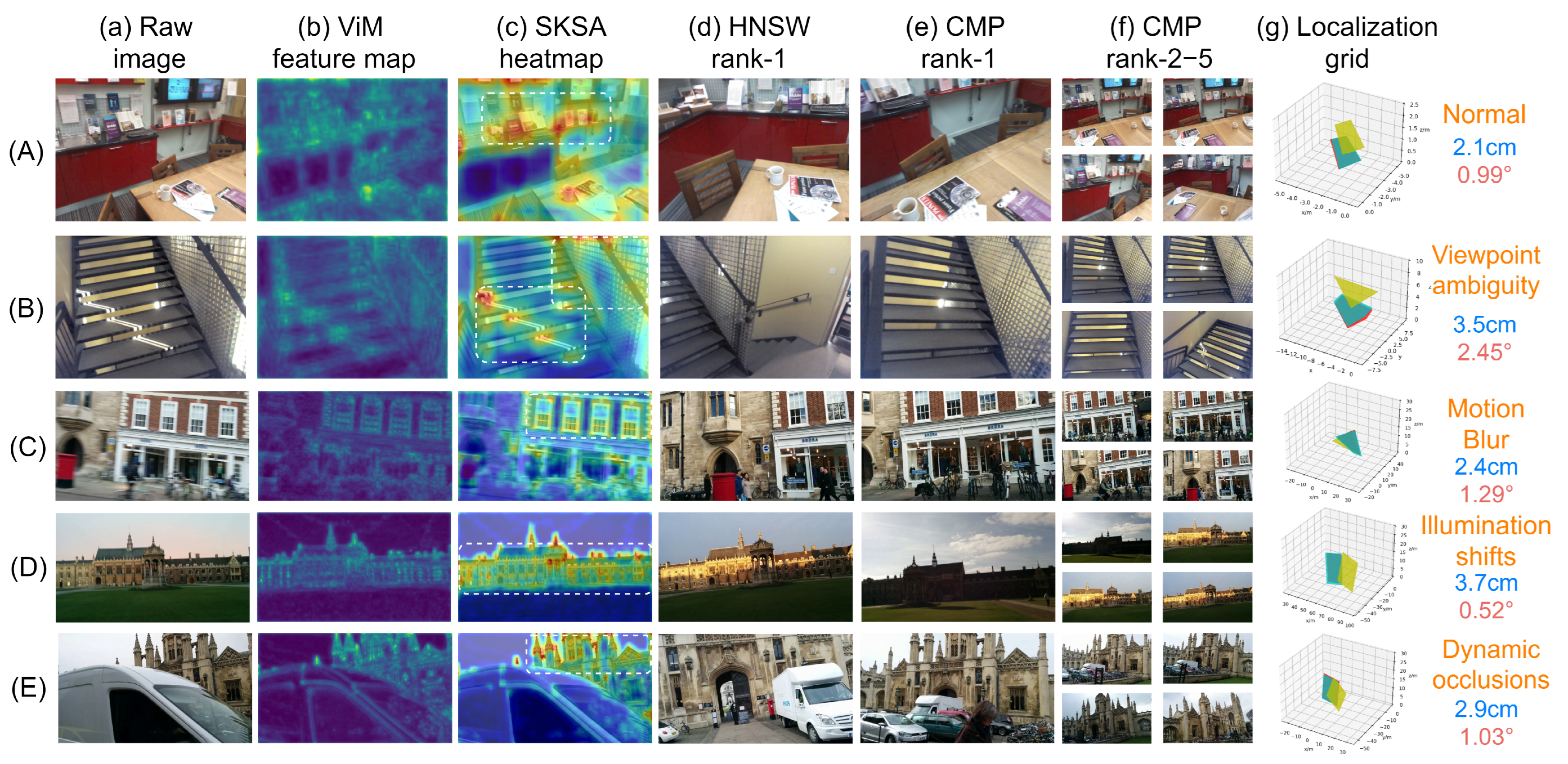
An illustration of DMT-Loc’s pipeline on representative queries from 7Scenes dataset (rows A,B) and Cambridge Landmarks dataset (rows C–E). From left to right: (a) raw image; (b) feature map from the ViM encoder; (c) attention heatmap from the SKSA module, with key regions highlighted by white dashed boxes; (d–f) retrieval results showing the top-1 match from HNSW (d), the re-ranked top-1 (e), and top-2–5 (f) matches from the CMP module; (g) 3D localization grid, with camera frustums indicating ground truth (red), nearest reference (yellow), and predicted pose (cyan). The main challenges and localization errors are indicated at the far right.
Figure 5.
An illustration of DMT-Loc’s pipeline on representative queries from 7Scenes dataset (rows A,B) and Cambridge Landmarks dataset (rows C–E). From left to right: (a) raw image; (b) feature map from the ViM encoder; (c) attention heatmap from the SKSA module, with key regions highlighted by white dashed boxes; (d–f) retrieval results showing the top-1 match from HNSW (d), the re-ranked top-1 (e), and top-2–5 (f) matches from the CMP module; (g) 3D localization grid, with camera frustums indicating ground truth (red), nearest reference (yellow), and predicted pose (cyan). The main challenges and localization errors are indicated at the far right.
Figure 6.
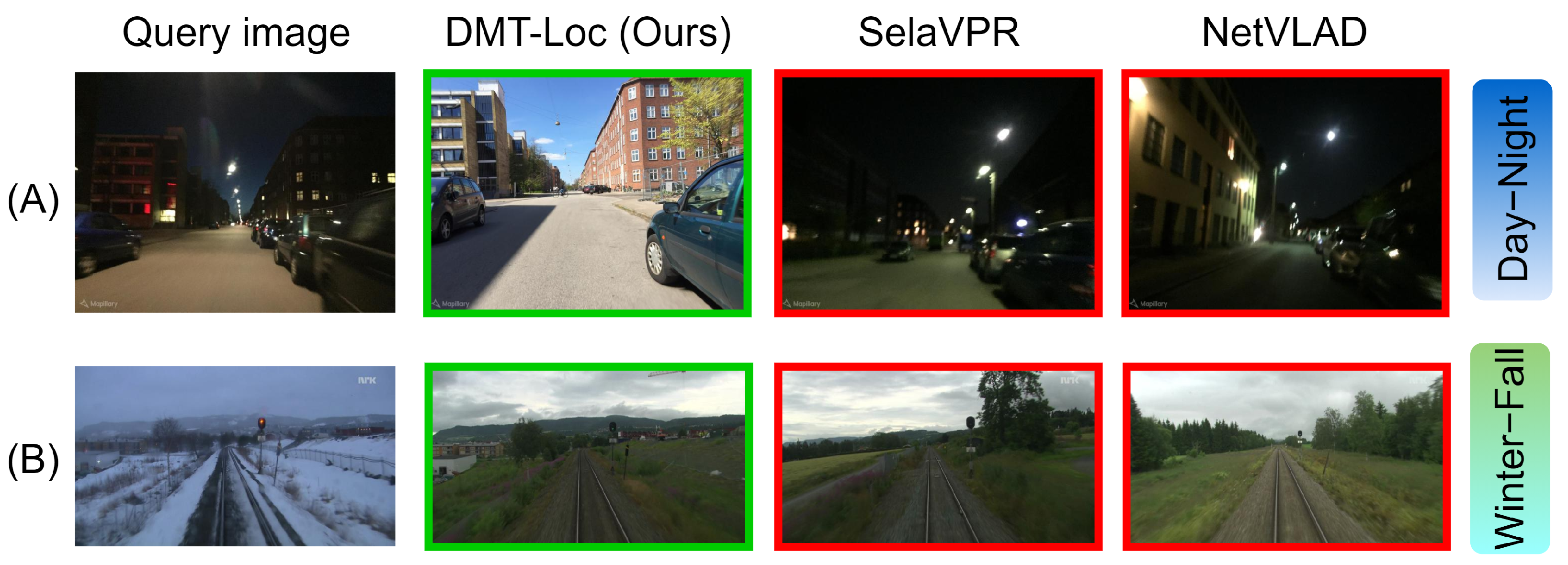
Rank-1 examples of VPR methods under challenging condition changes. (A) Query image from MSLS-challenge dataset with day–night transformation. (B) Query image from Nordland-test dataset with winter–fall transformation. Each method returns its most similar database image, with correct matches framed in green and incorrect matches in red.
Figure 6.
Rank-1 examples of VPR methods under challenging condition changes. (A) Query image from MSLS-challenge dataset with day–night transformation. (B) Query image from Nordland-test dataset with winter–fall transformation. Each method returns its most similar database image, with correct matches framed in green and incorrect matches in red.
Figure 7.
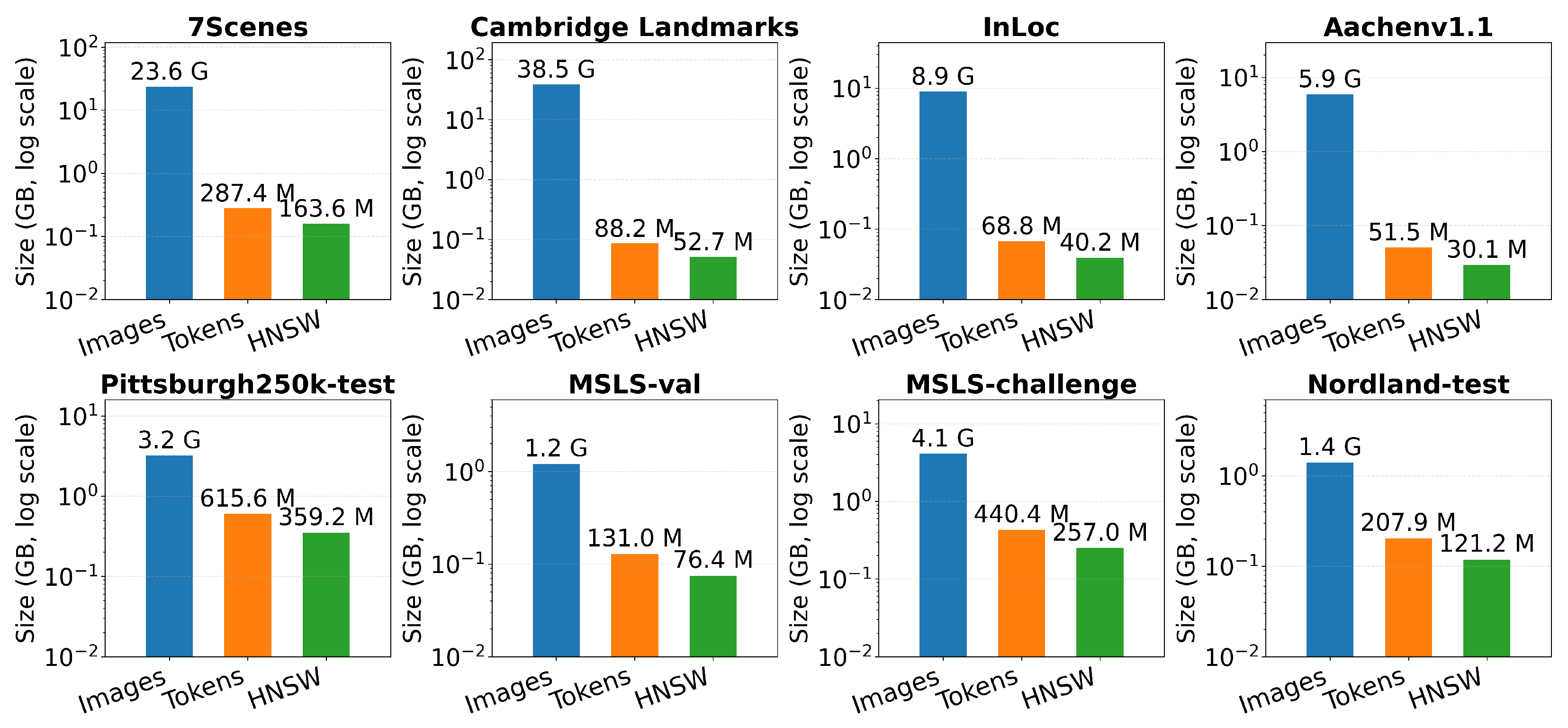
Storage efficiency of image tokenization across VL benchmarks with feature dimension 1536. The logarithmic y-axis scale intuitively reflects that the proposed method compresses raw datasets by orders of magnitude into compact tokens and HNSW graphs for efficient MFVR.
Figure 7.
Storage efficiency of image tokenization across VL benchmarks with feature dimension 1536. The logarithmic y-axis scale intuitively reflects that the proposed method compresses raw datasets by orders of magnitude into compact tokens and HNSW graphs for efficient MFVR.
Figure 8.
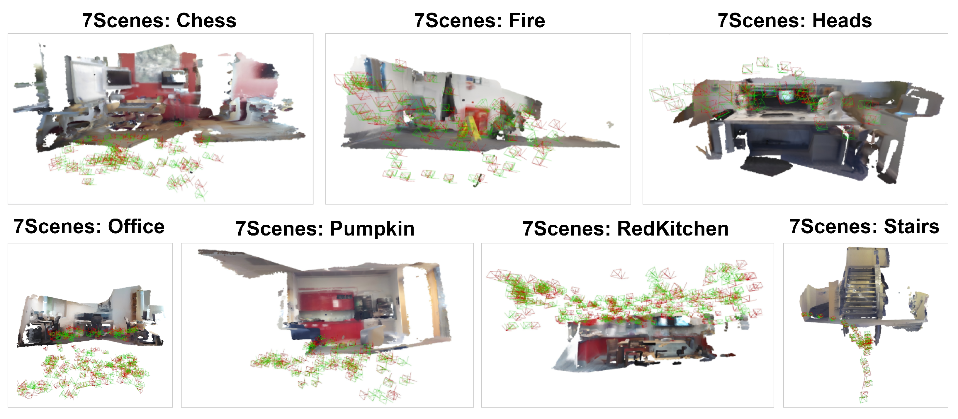
Qualitative results of camera calibration by DMT-Loc on the 7Scenes dataset. Each voxel map is reconstructed with 1000 frames per scene. Ground-truth and predicted 6DoF poses are visualized as red and green camera frustums, respectively.
Figure 8.
Qualitative results of camera calibration by DMT-Loc on the 7Scenes dataset. Each voxel map is reconstructed with 1000 frames per scene. Ground-truth and predicted 6DoF poses are visualized as red and green camera frustums, respectively.
Figure 9.
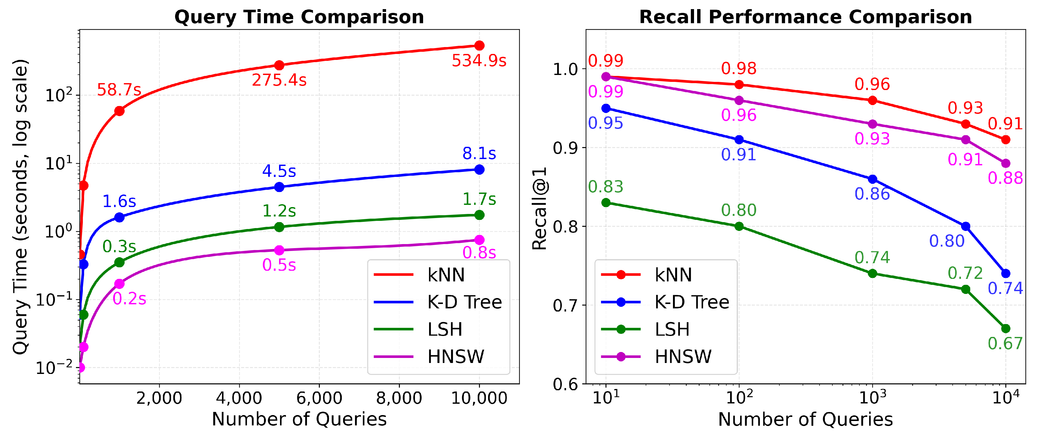
Performance comparison of IR algorithms on MSLS-challenge dataset. HNSW achieves the best trade-off between speed and accuracy.
Figure 9.
Performance comparison of IR algorithms on MSLS-challenge dataset. HNSW achieves the best trade-off between speed and accuracy.
Figure 10.
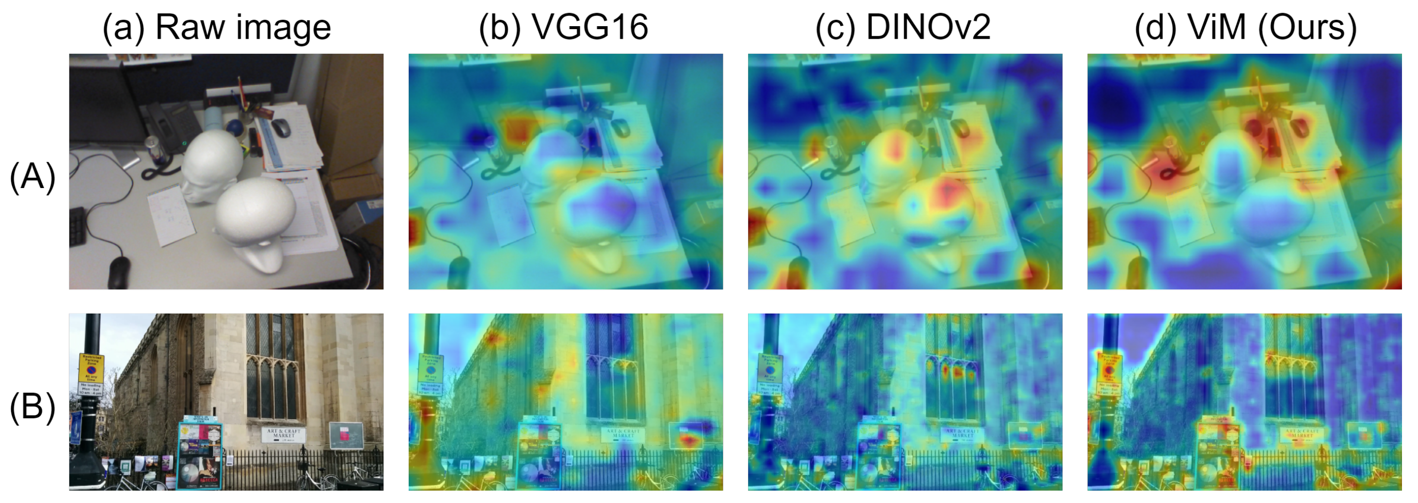
Attention heatmaps of visual encoders on indoor (A) and outdoor (B) scenes. (a–d) correspond to the raw images and heatmaps of VGG16, DINOv2, and ViM (ours), respectively. Warmer (cooler) colors correspond to higher (lower) attention.
Figure 10.
Attention heatmaps of visual encoders on indoor (A) and outdoor (B) scenes. (a–d) correspond to the raw images and heatmaps of VGG16, DINOv2, and ViM (ours), respectively. Warmer (cooler) colors correspond to higher (lower) attention.
Figure 11.
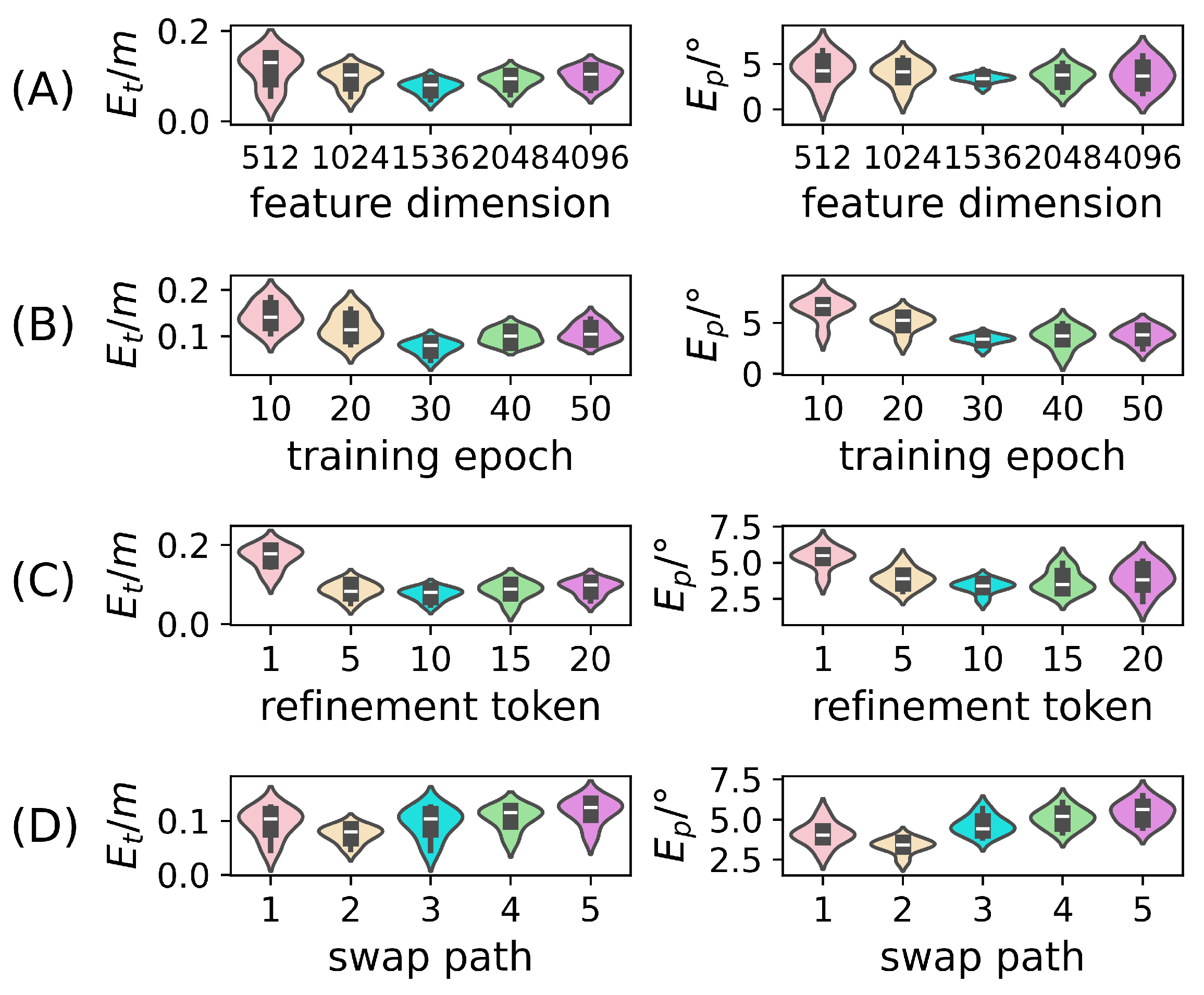
Systematic hyperparameter analysis of DMT-Loc: (A) feature dimension; (B) training epochs; (C) reference tokens; and (D) swap paths. The left and right columns reflect translation errors (m) and rotation errors (°), respectively. Optimal settings are highlighted: 1536 dimension, 30 epochs, 10 tokens, and 2 swap paths.
Figure 11.
Systematic hyperparameter analysis of DMT-Loc: (A) feature dimension; (B) training epochs; (C) reference tokens; and (D) swap paths. The left and right columns reflect translation errors (m) and rotation errors (°), respectively. Optimal settings are highlighted: 1536 dimension, 30 epochs, 10 tokens, and 2 swap paths.
Table 1.
Details of the adopted VL datasets. “★” and “✩” indicate presence and absence, respectively. Note that the MSLS dataset provides two distinct splits (i.e., MSLS-val and MSLS-challenge).
Table 1.
Details of the adopted VL datasets. “★” and “✩” indicate presence and absence, respectively. Note that the MSLS dataset provides two distinct splits (i.e., MSLS-val and MSLS-challenge).
| | Dataset | # Refer. | # Query | Motion | Light | Season | Occlusion |
|---|
| APE/RPE | 7Scenes [9] | 26.0k | 17.0k | ★★✩ | ★✩✩ | ✩✩✩ | ✩✩✩ |
| Cambridge [10] | 8.4k | 4.8k | ★★★ | ★★✩ | ✩✩✩ | ★★✩ |
| InLoc [41] | 10.0k | 329 | ★★✩ | ★★✩ | ✩✩✩ | ★★★ |
| Aachenv1.1 [42] | 6.7k | 1.0k | ★★✩ | ★★★ | ✩✩✩ | ★★★ |
| VPR | Pitts250k-test [12] | 83.9k | 8.2k | ★★✩ | ★★✩ | ★✩✩ | ★★✩ |
| MSLS-val [43] | 18.9k | 740 | ★★★ | ★✩✩ | ★★✩ | ★✩✩ |
| MSLS-challenge [43] | 38.8k | 27.1k | ★★✩ | ★★★ | ★★★ | ★★★ |
| Nordland-test [44] | 27.6k | 3.5k | ✩✩✩ | ★✩✩ | ★★★ | ✩✩✩ |
Table 2.
Median errors (cm/°) of baseline methods on benchmark VL datasets. “↓” indicates that lower values are better. Best RPR results are highlighted in bold and second best are underlined. Overall best results are marked in blue and second best are in green. “pw” and “mv” represent pair-wise and multi-view modes respectively. “–” means the value is unconverged or unobtainable. “†” means the method is unreproducible to our effort.
Table 2.
Median errors (cm/°) of baseline methods on benchmark VL datasets. “↓” indicates that lower values are better. Best RPR results are highlighted in bold and second best are underlined. Overall best results are marked in blue and second best are in green. “pw” and “mv” represent pair-wise and multi-view modes respectively. “–” means the value is unconverged or unobtainable. “†” means the method is unreproducible to our effort.
| | | 7Scenes (Indoor, Normal) ↓ | Cambridge Landmarks (Outdoor, Normal) ↓ |
|---|
| |
Method
|
Chess
|
Fire
|
Heads
|
Office
|
Pumpkin
|
Kitchen
|
Stairs
|
Average
|
College
|
Hospital
|
Shop
|
Church
|
Average-4
|
Court
|
|---|
| SbP | AS [23] | 4/2.00 | 3/1.50 | 2/1.50 | 9/3.60 | 8/3.10 | 7/3.40 | 3/2.20 | 5.1/2.47 | 42/0.60 | 44/1.00 | 12/0.40 | 19/0.50 | 29.3/0.63 | –/– |
| PixLoc [48] | 2/0.80 | 2/0.73 | 1/0.82 | 3/0.82 | 4/1.21 | 3/1.20 | 5/1.30 | 2.9/0.98 | 14/0.24 | 16/0.32 | 5/0.23 | 10/0.34 | 11.3/0.28 | 30/0.14 |
| DeViLoc [24] | 2/0.78 | 2/0.74 | 1/0.65 | 3/0.82 | 4/1.02 | 3/1.19 | 4/1.12 | 2.7/0.90 | 12/0.21 | 13/0.28 | 4/0.18 | 7/0.23 | 9.0/0.23 | 18/0.11 |
| FaVoR [49] | 1/0.20 | 1/0.40 | 1/0.60 | 2/0.40 | 1/0.30 | 1/0.30 | 6/1.60 | 1.9/0.50 | 18/0.30 | 27/0.50 | 5/0.30 | 11/0.40 | 15.3/0.38 | 29/0.20 |
| SCR | DSAC-star [25] | 2/1.10 | 2/1.24 | 1/1.82 | 3/1.15 | 4/1.34 | 4/1.68 | 3/1.16 | 2.7/1.36 | 18/0.30 | 21/0.40 | 5/0.30 | 15/0.60 | 14.8/0.40 | 49/0.30 |
| ACE [26] | 2/1.10 | 2/1.80 | 2/1.10 | 3/1.40 | 3/1.30 | 3/1.30 | 3/1.20 | 2.7/1.31 | 28/0.40 | 31/0.60 | 5/0.30 | 18/0.60 | 20.5/0.48 | 43/0.20 |
| NeuMap [50] | 2/0.81 | 3/1.11 | 2/1.17 | 3/0.98 | 4/1.11 | 4/1.33 | 4/1.12 | 3.1/1.09 | 19/0.14 | 36/0.19 | 25/0.06 | 53/0.17 | 33.3/0.14 | 10/0.06 |
| HSCNet++ [51] | 2/0.70 | 2/0.72 | 1/0.80 | 2/0.69 | 4/1.00 | 4/1.15 | 3/1.02 | 2.6/1.36 | 19/0.34 | 20/0.31 | 6/0.24 | 9/0.30 | 13.5/0.30 | 39/0.23 |
| D2S [52] | 2/0.57 | 2/0.74 | 1/0.75 | 2/0.62 | 3/0.83 | 3/1.04 | 13/2.02 | 3.7/0.94 | 7/0.12 | 15/0.29 | 3/0.17 | 8/0.25 | 8.3/0.21 | 23/0.11 |
| SACNet † [27] | 2/0.53 | 2/0.71 | 1/0.59 | 3/0.65 | 2/0.65 | 3/0.93 | 2/0.40 | 2.1/0.64 | 17/0.30 | 18/0.30 | 6/0.30 | 12/0.30 | 13.3/0.31 | 47/0.32 |
| APR | PoseNet [10] | 32/8.12 | 47/14.4 | 29/12.0 | 48/7.68 | 47/8.42 | 59/8.64 | 47/13.8 | 44.1/10.4 | 192/5.40 | 231/5.40 | 146/8.10 | 266/8.50 | 208.8/6.80 | –/– |
| PAE [53] | 12/4.95 | 24/9.31 | 14/12.5 | 19/5.79 | 18/4.89 | 18/6.19 | 25/8.74 | 18.6/7.48 | 90/1.49 | 207/2.58 | 99/3.88 | 164/4.16 | 140.0/3.03 | –/– |
| DFNet [54] | 5/1.88 | 17/6.45 | 6/3.63 | 8/2.48 | 10/2.78 | 22/5.45 | 16/3.29 | 12.0/3.71 | 73/2.37 | 200/2.98 | 67/2.21 | 137/4.03 | 119.3/2.90 | –/– |
| LENS † [28] | 3/1.30 | 10/3.70 | 7/5.80 | 7/1.90 | 8/2.20 | 9/2.20 | 14/3.60 | 8.3/2.96 | 33/0.50 | 44/0.90 | 27/1.60 | 53/1.60 | 39.3/1.15 | –/– |
| PMNet † [55] | 4/1.70 | 10/4.51 | 7/4.23 | 7/1.96 | 14/3.33 | 14/3.36 | 16/3.62 | 10.3/3.24 | –/– | –/– | –/– | –/– | –/– | –/– |
| Marepo [29] | 2/1.24 | 2/1.39 | 2/2.03 | 3/1.26 | 4/1.48 | 4/1.71 | 6/1.67 | 3.3/1.54 | –/– | –/– | –/– | –/– | –/– | –/– |
| RPR-pw | NN-Net [32] | 13/6.50 | 26/12.7 | 14/12.3 | 21/7.40 | 24/6.40 | 24/8.00 | 27/11.8 | 21.3/9.30 | –/– | –/– | –/– | –/– | –/– | –/– |
| ReLocNet [33] | 12/4.10 | 26/10.4 | 14/10.5 | 18/5.30 | 26/4.20 | 23/5.10 | 28/7.50 | 21.0/6.73 | –/– | –/– | –/– | –/– | –/– | –/– |
| AnchorNet [31] | 8/4.12 | 16/11.1 | 9/11.2 | 11/5.38 | 14/3.55 | 13/5.29 | 21/11.9 | 13.1/7.51 | 79/0.95 | 211/3.05 | 77/3.25 | 122/3.02 | 122.3/2.57 | 589/3.53 |
| NC-EssNet [34] | 12/5.60 | 26/9.60 | 14/10.7 | 20/6.70 | 22/5.70 | 22/6.30 | 31/7.90 | 21.0/7.50 | 61/1.60 | 95/2.70 | 71/3.40 | 112/3.60 | 84.8/2.80 | –/– |
| Map-free [56] | 9/2.66 | 13/4.54 | 11/4.81 | 11/2.77 | 16/3.11 | 14/3.48 | 18/4.70 | 13.1/3.72 | 244/2.54 | 373/5.23 | 97/3.17 | 291/5.10 | 251.3/4.01 | 840/4.56 |
| RelFormer [35] | 11/4.01 | 23/8.57 | 17/10.9 | 16/4.92 | 15/4.15 | 19/4.89 | 24/6.46 | 17.8/6.27 | 83/2.90 | 184/3.80 | 86/3.70 | 117/4.10 | 117.5/3.63 | 367/3.80 |
| DMT-Loc (Ours) | 8/3.59 | 7/3.53 | 4/2.60 | 9/3.81 | 8/3.55 | 9/3.51 | 6/2.19 | 7.3/3.25 | 23/1.19 | 18/1.02 | 9/0.87 | 12/0.98 | 15.5/1.02 | 24/0.94 |
| RPR-mv | CamNet † [57] | 4/1.73 | 3/1.74 | 5/1.98 | 4/1.62 | 4/1.64 | 4/1.63 | 4/1.51 | 4.0/1.69 | –/– | –/– | –/– | –/– | –/– | –/– |
| RelPoseGNN [36] | 8/2.70 | 21/7.50 | 13/8.70 | 15/4.10 | 15/3.50 | 19/3.70 | 22/6.50 | 16.1/5.24 | 48/1.00 | 114/2.50 | 48/2.50 | 152/3.20 | 90.5/2.30 | 320/2.20 |
| ReLoc3r [37] | 3/0.99 | 4/1.13 | 2/1.23 | 5/0.88 | 7/1.14 | 5/1.23 | 12/2.25 | 5.4/1.26 | 47/0.41 | 87/0.66 | 18/0.53 | 41/0.73 | 48.3/0.58 | 171/0.94 |
| DMT-Loc (Ours) | 2/0.74 | 3/0.95 | 2/1.18 | 4/0.72 | 5/0.97 | 4/1.16 | 4/1.80 | 3.6/1.12 | 9/0.54 | 8/0.56 | 5/0.37 | 6/0.44 | 7.0/0.48 | 11/0.39 |
Table 3.
Average accuracies (%) and training overheads of competitive methods on challenging VL datasets. “↑” indicates that higher values are better, and vice versa for “↓”. Overall best/second best results are marked in blue/green. Best/second best overheads are highlighted in bold/underlined.
Table 3.
Average accuracies (%) and training overheads of competitive methods on challenging VL datasets. “↑” indicates that higher values are better, and vice versa for “↓”. Overall best/second best results are marked in blue/green. Best/second best overheads are highlighted in bold/underlined.
| | | InLoc (Indoor, Difficult) | Aachenv1.1 (Outdoor, Difficult) | Training | Storage |
|---|
| | | Acc.@(0.25/0.5/1.0 m, 10°)↑ | Acc.@(0.25/0.5/5.0 m, 2/5/10°)↑ | Time↓ | Size↓ |
|---|
| |
Method
|
DUC1
|
DUC2
|
Day
|
Night
|
(Hours)
|
(GB)
|
|---|
| VPR | VLAD [13] | 0.20/12.5/18.7 | 0.30/13.8/19.1 | 0.00/0.10/22.8 | 0.00/1.00/19.4 | 18 | 5.2 |
| NetVLAD [12] | 8.20/24.7/48.9 | 6.40/26.3/54.9 | 0.00/0.20/18.9 | 0.00/0.00/14.3 | 30 | 4.8 |
| VLAD+In. [58] | 6.40/26.3/50.9 | 10.3/32.3/61.5 | 0.00/0.20/22.1 | 0.00/1.00/22.4 | 34 | 7.1 |
| APE | AS [23] | –/–/– | –/–/– | 85.3/92.2/97.9 | 39.8/49.0/64.3 | 60 | 3.2 |
| D2Net [59] | 44.4/58.6/71.2 | 31.3/49.6/67.9 | 84.8/92.6/97.5 | 84.7/90.8/96.9 | ≥72 | 22.3 |
| PixLoc [48] | 25.5/47.3/68.8 | 32.4/54.7/79.5 | 74.3/79.3/87.4 | 61.0/65.8/79.3 | ≥72 | 48.5 |
| HSCNet++ [51] | –/–/– | –/–/– | 72.7/81.6/91.4 | 43.9/57.1/76.5 | ≥72 | 27.4 |
| DeViLoc [24] | 55.8/63.8/88.9 | 61.0/72.5/89.4 | 87.4/94.8/98.2 | 87.8/93.9/100.0 | ≥72 | 15.9 |
| RPE | HLoc (SP+SG) [30] | 49.0/68.7/80.8 | 53.4/77.1/82.4 | 89.6/95.4/98.8 | 86.7/93.9/100.0 | – | 35.7 |
| RelFormer [35] | 51.5/73.7/86.4 | 55.0/74.0/81.7 | 60.2/67.1/78.5 | 51.4/62.5/73.5 | 27 | 8.5 |
| ReLoc3r [37] | 59.6/79.3/90.9 | 71.2/87.0/91.6 | 61.5/77.0/89.6 | 53.8/63.7/75.8 | 85 | 4.9 |
| DMT-Loc (Ours) | 64.9/84.8/91.3 | 75.6/88.3/92.8 | 88.7/95.0/98.3 | 86.2/91.8/99.5 | ≤2.5 | 0.2 |
Table 4.
Recall@1/5/10 (%) comparisons on VPR datasets. “↑” indicates that higher values are better. Best results are in bold and second best are underlined.
Table 4.
Recall@1/5/10 (%) comparisons on VPR datasets. “↑” indicates that higher values are better. Best results are in bold and second best are underlined.
| Method | Pitts250k-Test ↑ | MSLS-Val ↑ | MSLS-Challenge ↑ | Nordland-Test ↑ |
|---|
| NetVLAD [12] | 81.9/91.2/93.7 | 52.4/64.7/69.4 | 31.5/42.1/46.2 | 10.9/19.2/24.5 |
| DOLG [14] | 89.9/95.4/96.7 | 82.0/88.9/91.4 | 75.6/87.1/90.8 | 51.3/66.8/69.8 |
| CosPlace [17] | 88.4/94.5/95.7 | 82.8/89.7/92.0 | 61.4/72.0/76.6 | 54.4/69.8/75.9 |
| Patch-NetVLAD [15] | 87.5/94.5/96.0 | 79.5/86.2/87.7 | 48.1/57.6/60.5 | 44.9/50.2/52.2 |
| TransVPR [16] | 89.0/94.9/96.2 | 86.8/91.2/92.4 | 63.9/74.0/77.5 | 61.3/71.7/75.6 |
| MixVPR [18] | 91.5/95.5/96.3 | 88.0/92.7/94.6 | 64.0/75.9/80.6 | 58.4/74.6/80.0 |
| SelaVPR [20] | 92.7/98.0/98.9 | 87.7/95.8/96.6 | 69.6/86.9/90.1 | 47.2/66.6/74.1 |
| DMT-Loc (Ours) | 93.5/98.3/99.2 | 88.3/96.6/97.0 | 76.4/87.7/91.6 | 63.7/79.3/84.8 |
Table 5.
Median errors (cm/°) of different descriptors (transfered with GIPR) on 7Scenes and Cambridge Landmarks datasets. “↓” indicates that lower values are better. Best results are highlighted in bold and second best are underlined.
Table 5.
Median errors (cm/°) of different descriptors (transfered with GIPR) on 7Scenes and Cambridge Landmarks datasets. “↓” indicates that lower values are better. Best results are highlighted in bold and second best are underlined.
| | 7Scenes (Indoor, Normal) ↓ |
| Method | Chess | Fire | Heads | Office | Pumpkin | Kitchen | Stairs | Average |
| NetVLAD [12] | 17/8.47 | 19/10.3 | 14/11.2 | 23/10.1 | 24/10.8 | 21/10.0 | 18/6.27 | 19.4/9.58 |
| DOLG [14] | 43/11.5 | 43/13.2 | 25/14.6 | 40/17.5 | 35/11.1 | 54/15.0 | 30/7.79 | 38.6/12.9 |
| CosPlace [17] | 28/14.3 | 23/11.2 | 17/14.9 | 27/11.1 | 25/13.4 | 26/10.9 | 24/9.44 | 24.3/12.2 |
| Patch-NV [15] | 21/10.9 | 29/11.5 | 15/11.7 | 29/12.2 | 25/9.19 | 24/13.1 | 18/7.11 | 23.0/10.8 |
| MixVPR [18] | 24/14.3 | 17/10.6 | 16/12.4 | 33/16.9 | 23/10.7 | 27/9.64 | 19/7.03 | 22.7/11.6 |
| SelaVPR [20] | 26/15.1 | 22/16.8 | 15/14.7 | 32/19.5 | 21/13.6 | 37/21.4 | 16/8.90 | 24.1/15.7 |
| DMT-Loc (Ours) | 8/3.59 | 7/3.53 | 4/2.60 | 9/3.81 | 8/3.55 | 9/3.51 | 6/2.19 | 7.3/3.25 |
| | Cambridge Landmarks (Outdoor, Normal)↓ |
| Method | College | Hospital | Shop | Church | Average-4 | Court | Average-5 | Street |
| NetVLAD [12] | 182/5.40 | 109/5.12 | 66/8.28 | 150/10.3 | 127/7.28 | 621/15.9 | 226/9.00 | –/– |
| DOLG [14] | 392/6.73 | 218/6.01 | 291/10.4 | 416/10.7 | 329/8.46 | 969/17.3 | 457/10.2 | –/– |
| CosPlace [17] | 96/4.50 | 119/6.05 | 71/6.77 | 111/6.72 | 99/6.01 | 157/4.92 | 111/5.79 | –/– |
| Patch-NV [15] | 228/5.48 | 119/5.96 | 139/8.91 | 237/12.2 | 181/8.14 | 840/16.2 | 313/9.74 | 955/24.8 |
| MixVPR [18] | 61/4.52 | 46/4.27 | 32/4.77 | 48/9.43 | 47/5.75 | 56/5.88 | 49/5.77 | 356/24.3 |
| SelaVPR [20] | 59/5.95 | 48/5.09 | 37/5.83 | 51/7.52 | 49/6.10 | 64/6.17 | 52/6.11 | –/– |
| DMT-Loc (Ours) | 23/1.19 | 18/1.02 | 9/0.87 | 12/0.98 | 15.5/1.02 | 24/0.94 | 17/1.00 | 33/2.68 |
Table 6.
Average errors of scene-specific/agnostic RPR on 7Scenes and Cambridge Landmarks datasets. “↓” indicates that lower values are better. Best results are highlighted in bold and second best are underlined. “–” means the value is unconverged or unobtainable.
Table 6.
Average errors of scene-specific/agnostic RPR on 7Scenes and Cambridge Landmarks datasets. “↓” indicates that lower values are better. Best results are highlighted in bold and second best are underlined. “–” means the value is unconverged or unobtainable.
| | 7Scenes (m/°) ↓ | Cambridge (m/°) ↓ |
|---|
|
Method
|
Scene-Specific
|
Scene-Agnostic
|
Scene-Specific
|
Scene-Agnostic
|
|---|
| NN-Net [32] | 0.21/9.30 | 0.36/18.4 | –/– | –/– |
| ReLocNet [33] | 0.21/6.73 | 0.29/11.3 | –/– | –/– |
| EssNet [34] | 0.22/8.03 | 0.89/40.2 | 1.08/3.42 | 10.4/85.8 |
| NC-EssNet [34] | 0.21/7.50 | 0.82/26.2 | 0.85/2.83 | 7.98/24.4 |
| RelPoseGNN [36] | 0.16/5.24 | 0.36/13.6 | 1.68/3.60 | –/– |
| Relformer [35] | 0.18/6.27 | 0.30/8.53 | 1.37/2.30 | 3.35/10.7 |
| DMT-Loc-pw (Ours) | 0.07/3.25 | 0.16/6.09 | 0.17/1.00 | 1.59/4.36 |
| DMT-Loc-mv (Ours) | 0.03/1.12 | 0.22/7.65 | 0.08/0.46 | 0.59/0.72 |
Table 7.
Average errors ± standard deviations of DMT-Loc’s model components for ablation study on 7Scenes and Cambridge Landmarks datasets. “↓” indicates that lower values are better. Best results are highlighted in bold and second best are underlined. “✓” denotes module presence.
Table 7.
Average errors ± standard deviations of DMT-Loc’s model components for ablation study on 7Scenes and Cambridge Landmarks datasets. “↓” indicates that lower values are better. Best results are highlighted in bold and second best are underlined. “✓” denotes module presence.
| SKSA | TCDA | CMP | SSG | 7Scenes (m/°) ↓ | Cambridge (m/°) ↓ |
|---|
| ✓ | ✓ | ✓ | ✓ | 0.073 ± 0.017/3.25 ± 0.56 | 0.173 ± 0.061/1.00 ± 0.11 |
| | ✓ | ✓ | ✓ | 0.118 ± 0.032/5.53 ± 0.85 | 0.196 ± 0.096/1.99 ± 0.64 |
| ✓ | | ✓ | ✓ | 0.129 ± 0.045/4.96 ± 0.97 | 0.203 ± 0.112/2.12 ± 0.77 |
| ✓ | ✓ | | ✓ | 0.153 ± 0.086/7.82 ± 1.65 | 0.281 ± 0.177/3.47 ± 1.08 |
| ✓ | ✓ | ✓ | | 0.095 ± 0.028/4.18 ± 0.73 | 0.183 ± 0.079/1.75 ± 0.39 |
Table 8.
Average errors ± standard deviations of DMT-Loc’s design strategies for ablation study on 7Scenes and Cambridge Landmarks datasets. “↓” indicates that lower values are better. Best results are highlighted in bold and second best are underlined.
Table 8.
Average errors ± standard deviations of DMT-Loc’s design strategies for ablation study on 7Scenes and Cambridge Landmarks datasets. “↓” indicates that lower values are better. Best results are highlighted in bold and second best are underlined.
| Module | Technique | 7Scenes (m/°) ↓ | Cambridge (m/°) ↓ |
|---|
| Encoder | ViM | VGG16 | 0.129 ± 0.026/5.96 ± 0.89 | 0.396 ± 0.102/3.12 ± 0.77 |
| ResNet50 | 0.119 ± 0.023/5.42 ± 0.81 | 0.331 ± 0.094/2.75 ± 0.52 |
| DINOv2-ViT | 0.101 ± 0.022/4.66 ± 0.75 | 0.273 ± 0.083/2.45 ± 0.23 |
| DUSt3R | 0.096 ± 0.020/4.57 ± 0.72 | 0.315 ± 0.086/2.59 ± 0.44 |
| MxIT | SKSA | NLSA | 0.103 ± 0.028/4.74 ± 0.71 | 0.212 ± 0.085/1.82 ± 0.60 |
| w/o RBFConv | 0.097 ± 0.021/4.15 ± 0.66 | 0.195 ± 0.071/1.46 ± 0.29 |
| w/o Sparsemax | 0.085 ± 0.019/3.93 ± 0.61 | 0.188 ± 0.069/1.37 ± 0.43 |
| TCDA | VLAD | 0.144 ± 0.033/7.49 ± 1.15 | 0.744 ± 0.781/4.69 ± 1.72 |
| GeM | 0.156 ± 0.029/7.84 ± 0.91 | 0.971 ± 0.265/4.64 ± 1.09 |
| w/o Spatial | 0.142 ± 0.026/6.62 ± 1.03 | 0.251 ± 0.108/2.58 ± 0.82 |
| w/o Frequency | 0.096 ± 0.041/4.59 ± 1.15 | 0.207 ± 0.086/1.74 ± 0.93 |
| w/o Channel | 0.129 ± 0.025/5.13 ± 0.77 | 0.235 ± 0.097/2.05 ± 0.59 |
| DAR | HNSW | kNN | 0.076 ± 0.018/3.14 ± 0.58 | 0.174 ± 0.057/1.21 ± 0.16 |
| K-D Tree | 0.083 ± 0.024/3.82 ± 0.65 | 0.192 ± 0.074/1.48 ± 0.23 |
| LSH | 0.095 ± 0.029/4.37 ± 0.78 | 0.236 ± 0.092/1.86 ± 0.31 |
| CMP | Transformer Decoder | 0.183 ± 0.070/5.05 ± 1.34 | 0.238 ± 0.172/2.19 ± 0.85 |
| Mamba Decoder | 0.257 ± 0.182/7.49 ± 2.16 | 0.744 ± 0.781/4.69 ± 1.72 |
| Mamba Pointer | 0.092 ± 0.027/3.65 ± 0.61 | 0.194 ± 0.083/1.33 ± 0.26 |
| GIPR | SSG | w/o Gate | 0.121 ± 0.031/4.60 ± 0.79 | 0.214 ± 0.096/2.91 ± 0.68 |
| w/o Swap | 0.096 ± 0.027/3.97 ± 0.67 | 0.192 ± 0.084/1.73 ± 0.35 |
| w/o SiLU | 0.083 ± 0.023/3.49 ± 0.62 | 0.187 ± 0.082/1.65 ± 0.28 |
| | | DMT-Loc (Ours) | 0.073 ± 0.017/3.25 ± 0.56 | 0.173 ± 0.061/1.00 ± 0.11 |
Table 9.
Sensitivity analysis of modular hyperparameters. Sensitivity is reported as the maximum relative change in median pose errors (averaged over translation/rotation and both 7Scenes and Cambridge Landmarks datasets), varying each parameter within the tested range while keeping others at default. † Performance plateaus after 6 CMP layers.
Table 9.
Sensitivity analysis of modular hyperparameters. Sensitivity is reported as the maximum relative change in median pose errors (averaged over translation/rotation and both 7Scenes and Cambridge Landmarks datasets), varying each parameter within the tested range while keeping others at default. † Performance plateaus after 6 CMP layers.
| Symbol | Description | Equation | Default Value | Tested Range | Sensitivity |
|---|
| Gaussian kernel scale | Equation (2) | 1.0 | [0.5, 2.0] | <8% |
| Spatial scaling factor 1 | Equation (4) | 0.5 | [0.3, 0.7] | <5% |
| Spatial scaling factor 2 | Equation (4) | 2.0 | [1.5, 2.5] | <5% |
| Stability constant | Equation (7) | | {, } | <1% |
| k | Number of HNSW candidates | Equation (8) | 10 | [5, 20] | <6% |
| Number of CMP layers † | Equation (9) | 6 | [2, 10] | <10% |
| Loss balance coefficient 1 | Equation (12) | 1 | [0.5, 1.5] | <2% |
| Loss balance coefficient 2 | Equation (12) | 1 | [0.5, 1.5] | <4% |
Table 10.
Latency and memory for online RPR inference on a single image within 640 × 480 resolution. “↓” indicates that lower values are better. (FLOPs: floating point operations). Best results are highlighted in bold and second best are underlined.
Table 10.
Latency and memory for online RPR inference on a single image within 640 × 480 resolution. “↓” indicates that lower values are better. (FLOPs: floating point operations). Best results are highlighted in bold and second best are underlined.
| Method | Extraction | Regression | Params | FLOPs |
|---|
|
Latency (ms) ↓
|
Latency (ms) ↓
|
(MB) ↓
| (GB)↓ |
|---|
| NN-Net [32] | 40.19 | 8.41 | 47.32 | 87.6 |
| ReLocNet [33] | 41.80 | 9.32 | 75.30 | 116.4 |
| Relformer [35] | 106.47 | 18.92 | 291.45 | 359.8 |
| Map-free [56] | 31.71 | 11.20 | 87.26 | 107.1 |
| RelPoseGNN [36] | 72.63 | 28.28 | 204.41 | 284.2 |
| ReLoc3r [37] | 83.09 | 135.36 | 353.89 | 419.8 |
| DMT-Loc-pw (Ours) | 10.18 | 6.09 | 269.17 | 274.5 |
| DMT-Loc-mv (Ours) | 10.18 | 8.27 | 269.17 | 274.5 |



 ,
,