Tabular Data Distillation: An Extensive Comparison

Abstract

In this paper, we present an extensive evaluation of tabular data distillation methods for downstream classification and regression tasks. Our analysis considers multiple distillation approaches that are problem-type independent (i.e., unsupervised). For downstream learners, we focus on non-neural models such as Random Forest, XGBoost, and Support Vector Machines, as our goal is to evaluate the quality of the distilled data independently of the learner. The evaluation is conducted on 17 classification and nine regression problems. Our findings can be summarized as follows: (1) in all cases, applying a distillation method leads to a decrease in performance compared to the baseline; (2) overall, coreset-based methods are the most effective, with performance losses that are minimal—ranging from around 3% in classification accuracy or regression correlation to, in some cases, being negligible; (3) performance loss is moderately correlated with dataset tailness, measured as the proportion of outliers; (4) all distillation methods alter dataset consistency, narrowing the range of hyperparameter values that yield good performance; and (5) the Coreset Leverage Score remains fast, regardless of the size of the original set and of the distilled set.

1. Introduction

Dataset distillation, also known as dataset condensation, refers to the process of generating a small, highly informative subset from a large dataset such that a model trained on this subset achieves predictive performance comparable to that of a model trained on the original, full dataset [1,2,3]. Based on the traditional taxonomy [2], the distilled examples are synthetically generated to better capture the characteristics of the full dataset. A similar setup, but where the resulting instances were selected from the original dataset as key representatives, has been named instance selection [4,5] or instance reduction [6,7]. Recent studies [3,8] use distillation as an umbrella for all these methods, which reduces the original set size while preserving as much as possible of the performance, and we follow the same framework.

In terms of objectives and applications, dataset distillation helps reduce data storage requirements and can alleviate privacy and copyright concerns associated with maintaining and repeatedly using large volumes of raw data. Additionally, the smaller dataset size reduces the computational cost of model training, both in terms of runtime and memory usage, which is particularly beneficial when multiple models must be trained on the same dataset. These advantages enable a range of practical applications.

For example, in continual learning—where new tasks are learned sequentially while preserving knowledge of previous tasks—a “replay buffer” containing data from older tasks is often used to prevent catastrophic forgetting [9]. Dataset distillation can significantly reduce the memory requirements of such replay buffers, allowing models to learn a larger number of tasks without forgetting [10,11].

While dataset distillation has been extensively studied for image and prompt datasets [3,12], its application to other data modalities remains limited. In particular, tabular data distillation has received less attention, despite the fact that many real-world machine learning problems and applications rely on tabular data. This paper aims to fill this gap.

This paper makes the following contributions: (1) Presents an extensive comparison, with respect to downstream prediction, among unsupervised distillation methods for tabular data. (2) Identifies, surprisingly, the coreset methods as the strongest competitor, no matter the problem type (classification or regression) or learner or database used. (3) Identifies the Coreset Leverage Score method as offering the best compromise between performance, duration, and numerical robustness and G-Coreset (i.e., based on the Gonzales algorithm) as a tight competitor. (4) We identify a moderate correlation between distillation expected performance and a database tailness measure. (5) We emphasize the fact that distillation changes the database consistency, narrowing the range of hyperparameter values that yield good performance.

The remainder of the paper is organized as follows: Section 2 identifies previous studies on data distillation in general and on tabular data distillation in particular. In Section 3, we present the experimental chain; there, we present the learners, but most of it is dedicated to the distillation methods used. The datasets used are detailed in Section 5. Since the experimentation produced large amounts of raw results, we present those extensively in the Supplementary Materials and only integrative summaries in Section 6. We discuss the limitations of the proposed method in Section 8. The paper ends with a conclusion Section 9.

2. Related Work

The term ”dataset distillation” was coined by Wang et al. [2] and defines algorithms that “take as input a large real dataset to be distilled (training set), and outputs a small synthetic distilled dataset”. At the same time, a concurrent term, “dataset condensation”, was introduced by Zhao et al. [13] and it defines a method for ”training set synthesis for data-efficient learning, that learns to condense large dataset into a small set of informative synthetic samples”. Thus, the two techniques overlap in purpose and procedure.

The concept of making the training set smaller while keeping the same or most of the performance is older. As mentioned in the Introduction Section, instance selection [4,5] or instance reduction [6,7] were introduced as early as 2015. Yet in this paper, we refer to an even older algorithm, by Gonzales [14], which was introduced for clustering in 1985.

However, significant interest was garnered for compressing the training set by the very large data collection associated in modern times with deep learning. Methods in that direction work with an image database and a survey on the contributions may be followed in the work of Yu et al. [3] or for more general datasets (i.e., that include text data) in [15]. However, these studies approach trends and concepts in general without any focus on tabular data distillation.

Tabular data distillation has been examined in specific studies. For instance, Xu et al. [16] proposed a technique based on generative adversarial networks and one based on Variational Autoencoders. Zhao et al. [8] developed a method based on distribution matching where the distribution is estimated via representation in neural networks. Kang et al. [17] worked on the same idea, namely column embedding-based representation learning, but made the explicit assumption of an encoder’s existence. While these studies promote the proposed solution and include comparison against baseline, these comparisons are restricted to a few datasets and a few distillation methods.

In this work, we identify an existing gap in broad comparisons of distillation methods for tabular datasets and aim to fill it. To this end, we compare seven distillation techniques across 17 classification datasets and nine regression datasets, using three off-the-shelf learners and four different reduction ratios for the distilled datasets.

3. Methodology and Learners

3.1. Overview of Approach

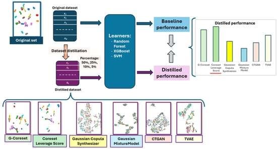
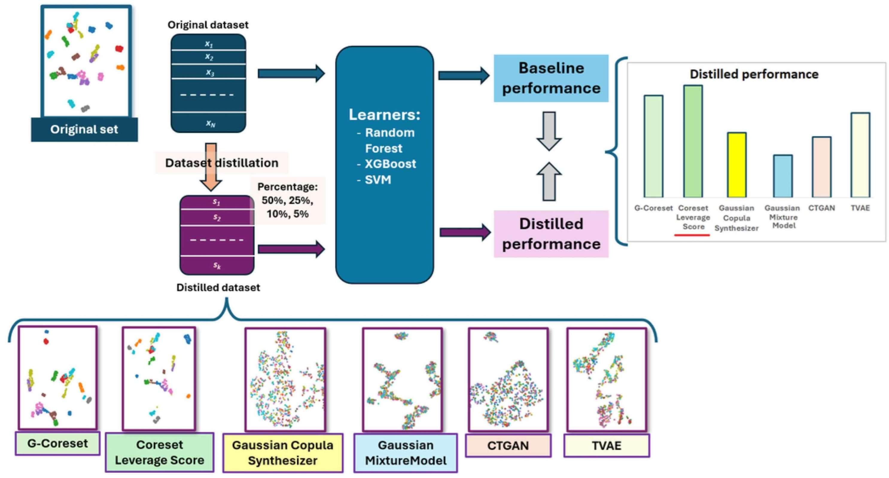
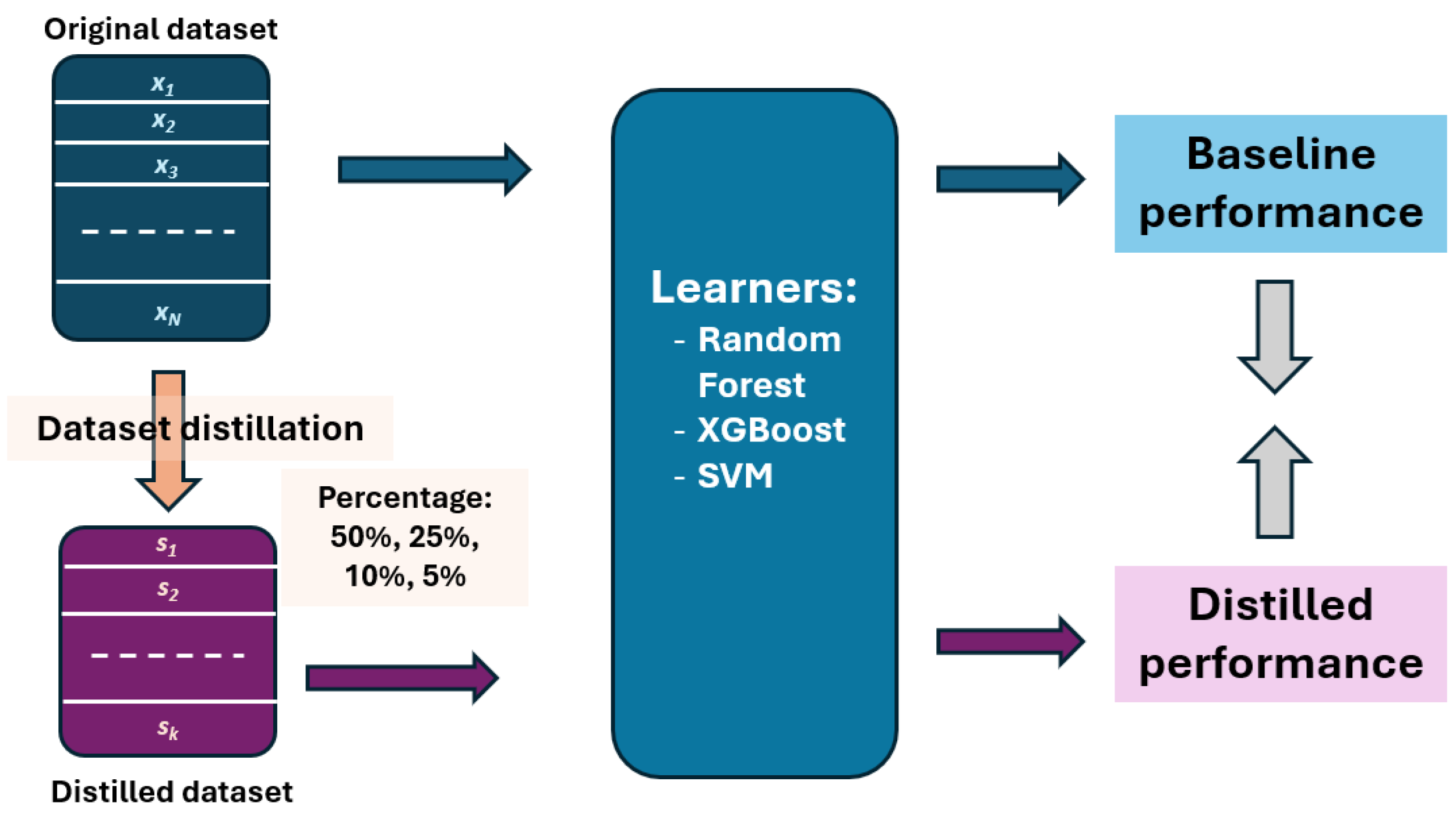
The general methodology (also shown in Figure 1) comprises the following key steps:

1.

Select a set of relevant tabular sets.

2.

Learner training and hyperparameter search.

3.

Select the distillation methods. Apply them on the tabular sets.

4.

Run the learners over the distilled/condensed datasets. Do hyperparameter search.

5.

Compare the performance on the distilled set with performance on the original set (baseline).

For the learning models, in all cases (distilled and original sets), training represents a single step within a broader exhaustive hyperparameter search. Each investigated hyperparameter configuration defines one complete training–testing cycle. In this study, we focus on Support Vector Machines (SVMs), Random Forests (RFs), and Gradient Boosting Machines, implemented using XGBoost. Details are presented below.

3.2. Formulation

Let the original dataset be represented by $\mathcal{X}$, containing n instances in a d-dimensional space: $\mathcal{X}=\{{\mathbf{x}}_1,{\mathbf{x}}_2,\dots ,{\mathbf{x}}_n\}$, where ${\mathbf{x}}_i\in {\mathbb{R}}^d$. An instance ${\mathbf{x}}_i$ has a label $y_i$ that can be either categorial for classification or continuous for regression problems. The learning problem is to find a model $f(·)$ that, when applied to the instance ${\mathbf{x}}_i$, will produce the prediction ${\hat{y}}_i$, which should be as close as possible to $y_i$.

The goal of a distillation method is to find a distilled set $\mathcal{S}$ consisting of k instances, where $k\ll n$: $\mathcal{S}=\{{\mathbf{s}}_1,{\mathbf{s}}_2,\dots {\mathbf{s}}_k\}$ with ${\mathbf{s}}_j\in {\mathbb{R}}^d$. In this context, each ${\mathbf{s}}_j$ acts as a “prototype” or distilled representative of a subset of the original data.

3.3. Learners

This study evaluates three widely used supervised learning algorithms: Random Forest (RF), Support Vector Machine (SVM), and Gradient Boosting Machine (GBM). These models are consistently reported as strong baselines for tabular learning. Earlier large-scale comparisons across many datasets identified RF and SVM among the most competitive methods [18]. More recent studies further show that gradient boosting approaches, particularly implementations such as XGBoost, achieve state-of-the-art performance on tabular data [19].

Recent broad empirical analyses confirm that tree-based methods remain highly competitive for tabular learning. For example, Grinsztajn et al. [20] demonstrate that classical tree ensembles often outperform deep learning approaches on typical tabular datasets, while more recent work [21] provides both empirical and theoretical insights supporting the robustness of non-deep models in this domain. Based on these findings, we focus on RF, SVM, and XGBoost as representative and competitive learners for tabular tasks.

Although ensemble methods such as RF and GBM are naturally robust due to averaging and randomized feature selection [22], careful hyperparameter tuning remains necessary to obtain strong performance. Because optimal hyperparameters are dataset-dependent and cannot be determined a priori [23,24], we employ a grid search to explore combinations of candidate values and select configurations that maximize predictive performance.

3.3.1. Random Forest

Random Forest(RF) [25] is a learner that operates on the principle of Bagging and Feature Randomness. As an ensemble method, Random Forest aggregates predictions from multiple decision trees trained on different bootstrap samples.

Each tree in the forest is a tree grown using the CART (Classification and Regression Trees) algorithm. A tree partitions the feature space into disjoint regions. For a given node, the algorithm seeks the best split by minimizing an impurity measure (for classification) or variance (for regression).

For a region $R_m$, the prediction is typically the average or majority value of the training observations ${\mathbf{x}}_i\in R_m$:

$${\hat{y}}_{R_m}=\mathrm{aggregate}\left(\{y_i:{\mathbf{x}}_i\in R_m\}\right)$$

(1)

Random Forest introduces two layers of randomness to create a diverse “forest”. The first layer is Bootstrap Sampling: for each tree, a random sample $\mathbf{X}$ of size ”in-bag percentage” is drawn with replacement from the original training data. The second layer is Feature Subspacing: at each node of every tree, the algorithm selects a random subset of $p<d$ features and chooses the best split only from this subset.

The forest model F is a collection of B trees. The final prediction in the case of classification is determined by a majority vote. For regression problems, the final prediction is the average of the numerical outputs of all trees.

The key hyperparameters we tuned were the in-bag percentage and the number of features, p, considered at each split; performance is not convex with respect to these two parameters. Although the number of trees can also influence performance, accuracy generally increases monotonically (though not strictly) with the number of trees until saturation.

3.3.2. Gradient Boosting Machine

The Gradient Boosting Machine is implemented using eXtreme Gradient Boosting (XGBoost) [26], an optimized variant of the original Gradient Boosting framework [27]. XGBoost is an ensemble learning method that combines multiple weak learners—typically trees—into a strong predictive model. Each tree is trained to correct the residual errors of the preceding ensemble, a process known as boosting.

Mathematically, XGBoost is an iterative procedure that begins with an initial prediction (commonly zero) and incrementally adds trees to minimize prediction error. This process can be formalized as:

$$\widehat{y_i}=\sum _{m=1}^M{f}_m\left({\mathbf{x}}_i\right)$$

(2)

where $\widehat{y_i}$ is the final predicted value for the i-th instance, ${\mathbf{x}}_i$, M is the total number of trees in the ensemble, and $f_m\left({\mathbf{x}}_i\right)$ is the prediction of the m-th tree.

The objective function in XGBoost consists of two components: a loss function, which measures how well the model fits the training data, and a regularization term, which penalizes model complexity to prevent overfitting. Its general form is:

$$\mathcal{L}\left(\theta \right)=\sum _{i=1}^{n}l(y_i,\widehat{y_i})+\sum _{m=1}^M\mathsf{\Omega }\left(f_m\right)$$

(3)

where $l(y_i,\widehat{y_i})$ quantifies the error between the true value $y_i$ and the prediction $\widehat{y_i}$, and $\mathsf{\Omega }\left(f_k\right)$ penalizes overly complex trees.

In our case, cross-entropy as $l(·)$ is used for classification and Mean Squared Error for the regression task. The hyperparameters tuned in our implementation were the learning rate, the minimum number of samples required to create a child node, and the subsampling ratio.

3.3.3. Support Vector Machine

Support Vector Machine (SVM) [28] performs strongly on tabular data, particularly on weak or noisy feature sets. They are among the most robust and mathematically grounded algorithms in machine learning.

Support Vector Machines (SVMs) aim to find the maximum-margin hyperplane separating two classes. Given the dataset $\mathcal{X}$ with labels $y_i\in \{-1,1\}$, the decision function is:

$$f\left(\mathbf{x}\right)={\mathbf{w}}^T\mathbf{x}+b\gtrless 0$$

(4)

The optimal hyperplane maximizes the margin between classes, which is equivalent to minimizing the norm of the weight vector:

$$\underset{\mathbf{w},b}{min}{\displaystyle \frac{1}{2}}{\parallel \mathbf{w}\parallel }^2,\mathrm{subject}\mathrm{to}\text{:}{y}_i({\mathbf{w}}^T{\mathbf{x}}_i+b)\ge 1$$

(5)

For non-separable data, slack variables ${\xi }_i$ are introduced and controlled by a regularization parameter C (named cost).

To handle non-linear boundaries, SVM employs the kernel trick, mapping data into a higher-dimensional space through a kernel function:

$$K({\mathbf{x}}_i,{\mathbf{x}}_j)=\varphi {\left({\mathbf{x}}_i\right)}^T\varphi \left({\mathbf{x}}_j\right)$$

(6)

Following the recommendations of LibSVM [29], we use the radial basis function (RBF) kernel: $K(\mathbf{x},\mathbf{z})=exp(-\gamma \parallel \mathbf{x}-\mathbf{z}{\parallel }^2)$. For multi-class classification, we adopt the One-vs-Rest strategy [29].

For the regression problem, Support Vector Regression (SVR) is used. Instead of keeping points out of a margin, SVR tries to fit as many points as possible within a margin (the $ϵ$-insensitive tube). The objective is to find a function $f\left(\mathbf{x}\right)={\mathbf{w}}^T\mathbf{x}+b$ that deviates from the actual targets $y_i$ by no more than $ϵ$. The optimization minimizes:

$${\displaystyle \frac{1}{2}}{\parallel \mathbf{w}\parallel }^2+C\sum _{i=1}^n({\xi }_i+{\xi }_i^{*})\mathrm{subject}\mathrm{to}\text{:}|y_i-({\mathbf{w}}^T\mathbf{x}+b)|\le ϵ+{\xi }_i$$

(7)

Errors smaller than $ϵ$ are ignored, making the model robust to noise and outliers that fall within the tube.

In our experiments, we used an aggregated one-vs-all formulation with a Gaussian (RBF) kernel. Following the recommendations in the LibSVM documentation [29], the hyperparameters we tuned were the cost parameter (which regulates the trade-off between margin width and classification errors) and the variance of the Gaussian kernel, $\gamma$, which controls the curvature of the decision boundary.

4. Distillation Methods

Fundamentally, distillation methods can be divided according to the following criteria:

• Realism

  –

  Instance selection [4]: Methods that select existing instances.

  –

  Generator: Methods that generate new, synthetic instances. They follow the standard distillation taxonomy [2].

• Objective

  –

  Distribution matching: The purpose is to produce examples that match the original population statistics. Statistics can be evaluated by:

  *

  Low order moments, such as mean, variance;

  *

  Low order moments and outliers.

  Actual methods, here, include:

  *

  Moments matching: Mean, covariance, skewness, kurtosis.

  *

  Gaussian Mixture Models (GMMs).

  *

  Copula-based synthetic data generators.

  *

  Probability distribution fitting.

  –

  Gradient matching: This create a small synthetic dataset whose gradients (with respect to a model) match those produced by the real dataset. However, they are dependent on the learning model and, thus, not used in this study.

  –

  Label-Preserving Condensation: It focuses on label distribution, $P\left(Y\right)$, preservation instead of data distribution, $P\left(X\right)$.

We aim to evaluate learner independent, label independent methods. Thus, we restricted our evaluation on a limited set that will be detailed in the next subsections.

4.1. K-Means

As a distillation method, K-means [30,31] may be seen as a distribution matching method where the distilled set fits the mean of clusters from the original set. Formally, the K-means algorithm seeks to partition the original n observations into k sets $C=\{C_1,C_2,\dots ,C_k\}$ so as to minimize the within-cluster sum of squares.

The distilled instances (centroids), ${\mathbf{s}}_j$ are defined by the following optimization:

$$\underset{C}{\mathrm{argmin}}\sum _{j=1}^k\sum _{{\mathbf{x}}_i\in C_j}{\parallel {\mathbf{x}}_i-{\mathbf{s}}_j\parallel }^2$$

(8)

The distilled instance ${\mathbf{s}}_j$ is calculated as the mean of the points assigned to that cluster:

$${\mathbf{s}}_j={\displaystyle \frac{1}{|C_j|}}\sum _{{\mathbf{x}}_i\in C_j}{\mathbf{x}}_i$$

(9)

Naturally, the mean is unlikely to be a point existing initially in the set, ${\mathbf{s}}_j\notin \mathcal{X}$. Thus, as an alternative to K-means, one might use K-Medoids [32]. While both aim to divide a dataset into k groups, the fundamental difference lies in how they define the “center” of a cluster. In K-Medoids, the center of a cluster, called a medoid, is an actual data point from the original dataset. Specifically, it is the point within a cluster that has the minimum total dissimilarity to all other points in that same cluster.

4.2. Coreset Methods

A coreset is defined [33,34] as small weighted or unweighted subset of the original dataset such that training (or evaluating) a model on the coreset approximates training on the full dataset. In general, coreset methods select real data points (as opposed to creating synthetic points), aim to preserve geometry/coverage/influence of the data set, and thus are especially natural for tabular data [34]. In contrast to K-means, distilled points are from the original dataset ${\mathbf{s}}_j\in \mathcal{X}$.

In this evaluation, we consider two alternatives: one based on the Gonzales algorithm [14], named G-Coresets, and one based on Leverage Score.

4.2.1. G-Coreset

The Gonzalez algorithm [14] is a greedy strategy designed to solve the K-Center problem. It distills data by iteratively picking the instance that is furthest from the currently selected set, ensuring the “maximum coverage” of the data space.

The objective is then formulated as the minimization of the maximum distance between any point in $\mathcal{X}$ and its nearest neighbor in the distilled set $\mathcal{S}$:

$$\underset{S\in \mathcal{X},\left[S\right]=k}{min}\underset{{\mathbf{x}}_i\in \mathcal{X}}{max}\mathrm{dist}({\mathbf{x}}_i,\mathcal{S})$$

(10)

where $\mathrm{dist}({\mathbf{x}}_i,\mathcal{S})={min}_{{\mathbf{s}}_j\in \mathcal{S}}\parallel {\mathbf{x}}_i-{\mathbf{s}}_j\parallel$

The distillation process, further named G-Coreset (Gonzales Coreset), is built with a greedy iterative algorithm:

• Initialize: Pick an arbitrary starting point ${\mathbf{s}}_1\in \mathcal{X}$. Set $S_1=\left\{s_1\right\}$.
• Iterate: For $t=2$ to k:

  –

  Find the instance ${\mathbf{x}}_i\in \mathcal{X}$ that is furthest from the current set $S_{t-1}$:

  $${\mathbf{s}}_t=\underset{{\mathbf{x}}_i\in \mathcal{X}}{\mathrm{argmax}}\left(\underset{\mathbf{s}\in S_{t-1}}{min}\parallel {\mathbf{x}}_i-\mathbf{s}\parallel \right)$$

  (11)

  –

  Update the distilled set: $S_t=S_{t-1}\cup \left\{{\mathbf{s}}_t\right\}$.

• Result: The final set $S_k$ is an approximate coreset for the K-Center objective.

Following this algorithm, $\mathcal{S}=S_k$. Equation (11) ensures that the set maximizes the coverage.

4.2.2. Coreset Leverage Score

An alternative to Gonzales’ method is Leverage Score sampling for the coreset. The method is built in the context of linear regression, where not all data points contribute equally to the final model; some points, known as high-leverage points, have a disproportionate influence on the position of the regression line. By identifying and prioritizing these points, we can distill a dataset that maintains the predictive power of the original, while significantly reducing the computational overhead.

The statistical core of this method lies in the projection (or “hat”) matrix. For a dataset $\mathcal{X}$ with N samples and d features, the Leverage Score ${\psi }_i$ for each observation ${\mathbf{x}}_i$ is defined as:

$${\psi }_i={\mathbf{x}}_i^T{\left({\mathcal{X}}^T\mathcal{X}\right)}^{-1}{\mathbf{x}}_i$$

(12)

These scores correspond to the diagonal elements of the hat matrix $H=\mathcal{X}{\left({\mathcal{X}}^T\mathcal{X}\right)}^{-1}{\mathcal{X}}^T$. Geometrically, ${\psi }_i$ measures how far an individual observation’s features are from the average of the features in the dataset. A high Leverage Score indicates that the point is an outlier in the feature space and, consequently, plays a critical role in defining the model’s parameters.

To perform the distillation, points are sampled with a probability proportional to their Leverage Scores. This process ensures that “important” points are preserved in the distilled coreset. This approach provides strong theoretical guaranties. Specifically, if we sample m points where $m\ll n$, the resulting model trained on the distilled data will be a $(1+ϵ)$ approximation of the model trained on the full dataset.

However, we emphasize that this theoretical justification is valid only in the context of linear least-squares problems and low-rank matrix approximation. The guarantees concern subspace preservation and approximation of linear objectives. Since the downstream learners are non-linear, the toretical guarantees do not transfer directly to RF, XGB, or RBF-SVM.

In practice, directly computing the hat matrix H is very computationally intensive since it requires multiplication over the entire dataset. Based on the work of Drineas et al. [35], we first compute a rank-k approximation of $\mathcal{X}$ using Principal Component Analysis (PCA). Based on the Singular Value Decomposition (SVD), fundamental result, $\mathcal{X}=U\Sigma V^T$, where $U\in {\mathbb{R}}^{N\times N}$, $\Sigma \in {\mathbb{R}}^{N\times d}$, $V\in {\mathbb{R}}^{d\times d}$.

Now let $U_m\in {\mathbb{R}}^{N\times m}$ to denote the matrix formed by the top-m left singular vectors corresponding to the largest singular values. The Leverage Score may be computed as:

$${\psi }_i={∥{\left(U_m\right)}_{i,:}∥}_2^2$$

(13)

where ${\left(U_m\right)}_{i,:}$ is the i-th row of $U_m$. We recall [35,36] that ${\psi }_i\ge 0$ and ${\sum }_{i=1}^N{\psi }_i=m$, while high Leverage Scores indicate influential or extreme samples, which are relevant in forming coresets.

We define a probability distribution over samples:

$$p_i={\displaystyle \frac{{\psi }_i}{{\sum }_{j=1}^N{\psi }_j}}={\displaystyle \frac{{\psi }_i}{m}}$$

(14)

Given a target reduced size $k\ll N$, we sample k rows without replacement according to:

$${\mathcal{X}}_S\sim \mathrm{Multinomial}(k,{\left\{p_i\right\}}_{i=1}^n)⟹\mathcal{S}=\{{\mathbf{s}}_i\mid i\in {\mathcal{X}}_S\}$$

(15)

From an intuitive point of view, we apply PCA-based Leverage Score sampling to select informative samples. Leverage Scores are computed from the top principal components and used to define a sampling distribution over data points.

4.3. Copula Based Distillation

We recall that a copula is a multivariate cumulative distribution function for which the marginal probability distribution of each variable is uniform on the interval $[0,1]$. The development of copulas in practical application is based on Sklar theorem [37], which states that every multivariate cumulative distribution function can be expressed in terms of its marginals and a copula $C(·)$.

To build an actual copula-based distillation method, we consider that each instance ${\mathbf{x}}_i$ is a vector of d random variables $(X^{\left(1\right)},X^{\left(2\right)},\dots ,X^{\left(d\right)})$. According to Sklar’s theorem, the joint cumulative distribution function (CDF) can be decomposed:

$$F\left(x^{\left(1\right)},\dots ,x^{\left(d\right)}\right)=C\left(F^1\left(x^{\left(1\right)}\right),\dots ,F^d\left(x^{(d)}\right)\right)$$

(16)

where $F^j$ is the marginal CDF on the j-th dimension and $C(·)$ is the Copula function describing the dependency structure.

While different models may be used, previous distillation and synthesis studies [38,39] used a Gaussian Copula model. It assumes that dependencies between features follow a multivariate normal structure:

$$C_{\Sigma }(u_1,\dots u_d)={\Phi }_{\Sigma }({\Phi }^{-1}\left(u_1\right)\dots {\Phi }^{-1}\left(u_d\right))$$

(17)

where ${\Phi }^{-1}$ is the inverse CDF (quantile function) of the standard normal distribution, and ${\Phi }_{\Sigma }$ is the joint CDF of a multivariate normal distribution with mean 0 and correlation matrix $\Sigma$.

The distillation (synthesis) process [40] works as follows:

• Marginal Estimation: For each dimension j, estimate the empirical CDF ${\hat{F}}^j\approx F^j$ from the original data $\mathcal{X}$.
• Correlation Inference: Transform the original data into a latent Gaussian space and calculate the correlation matrix $\Sigma$:

  $$z_{i,j}={\Phi }^{-1}\left({\hat{F}}^j\left(x_{i,j}\right)\right)⟹\Sigma =Cov\left(Z\right)$$

  (18)
• Sampling (Distillation): Generate k synthetic samples in the latent space:

  $${\psi }_k\sim \mathcal{N}(0,\Sigma ),k=1\dots ,k$$

  (19)
• Inverse Transformation: Map the samples back to the original data space:

  $$s_{k,j}={\hat{F}}_j^{-1}(\Phi \left({\psi }_{k,j}\right))$$

  (20)

While K-means distills data into “average” points, the coreset does it in border points and the Gaussian Copula distills the “rules” of the data (distribution and correlation). By sampling k times from this learned model, one obtains a distilled set S that mimics the original density and feature relationships.

The solution used in this study is based on the SDV library [40].

4.4. Gaussian Mixture Model

Data distillation via distribution matching aims to create a synthetic set $\mathcal{S}$ such that the statistical distribution of $\mathcal{S}$ is as close as possible to the distribution of the original dataset $\mathcal{X}$. By using Gaussian Mixture Models (GMMs), we can represent $\mathcal{X}$ as a combination of m probability densities and use the parameters of these densities to derive our k distilled instances.

In this framework, we assume $\mathcal{X}$ is generated by a probability density function $P\left(\mathcal{X}\right)$. We model this density using a GMM with m components:

$$P\left(\mathbf{x}\right|\theta )=\sum _{j=1}^m{\pi }_j\mathcal{N}\left(\mathbf{x}\right|{\mu }_j,{\Sigma }_j)$$

(21)

where $\theta =\{{\pi }_j,{\mu }_j,{\Sigma }_j\}$ are the parameters of the mixture model, ${\pi }_j$ is the mixing coefficient for the j-th component (${\sum }_{j=1}^m{\pi }_j=1$), and $\mathcal{N}\left(\mathbf{x}\right|{\mu }_j,{\Sigma }_j)$ is the multivariate Gaussian distribution with mean ${\mu }_j$ and covariance ${\Sigma }_j$.

The distribution is iteratively found using an Expectation-Maximization algorithm. First, one needs to find the parameters $\theta =\{{\pi }_j,{\mu }_j,{\Sigma }_j\}$, $j=1\dots m$ that maximize the likelihood of the original data $\mathcal{X}$:

$$logP\left(\mathbf{x}\right|\theta )=\sum _{i=1}^{N}log\left(\sum _{j=1}^m{\pi }_j\mathcal{N}\left(\mathbf{x}\right|{\mu }_j,{\Sigma }_j)\right)$$

(22)

Once the modes are found, they are sampled k times to retrieve the distilled set $\mathcal{S}$:

$${\mathbf{s}}_j\sim \mathcal{N}\left(\mathbf{x}\right|{\mu }_j,{\Sigma }_j),j=1,\dots ,k$$

(23)

4.5. Conditional Tabular GAN

More recent and elaborated models have used deep architectures to synthesize data that should match a given set. In this work, we focus on the Conditional Tabular GAN (CTGAN) solution by Xu et al. [16]. The solution is a modified generative adversarial network specifically designed to produce high-quality synthetic tabular data.

In more detail, the CTGAN is designed to adapt to modeling tabular data, which often contain mixed-type columns, non-Gaussian distributions, and imbalanced categorical values. Off-the-shelf deep learning models often fall short because tabular data does not share the local structures found in images or text. To address these challenges, CTGAN implements three primary changes:

1.

Mode-Specific Normalization for Continuous Columns. It starts from the observation that continuous columns in tabular data are often non-Gaussian and multimodal, meaning they have multiple “peaks” or modes in their distribution, which CTGAN addresses through mode-specific normalization. It uses a Variational Gaussian Mixture (VGM) model to estimate the number of modes and fit a Gaussian mixture to each continuous column. Each value is transformed into a representation consisting of a one-hot vector (indicating which mode the value belongs to) and a scalar (representing the value’s normalized position within that specific mode). This allows the model to focus on learning the distribution within each mode independently.

2.

Conditional Generator and Training-by-Sampling. It starts from the observation that categorical columns are frequently highly imbalanced, where a single category might appear in over 90% of the rows. In the standard GAN training, the generator may never learn to produce rare “minority” classes because they do not appear enough to influence the discriminator. CTGAN solves this using a conditional generator and a “training-by-Sampling” approach: The generator is given a conditional vector that specifies a particular category from a discrete column that it must produce; then, during training, CTGAN samples categories based on the logarithm of their frequency rather than their raw frequency. This forces the model to “evenly explore” and learn from minority categories that would otherwise be ignored. Next, a cross-entropy loss is added to the generator to penalize it, if the generated row does not match the requested condition.

3.

Specialized Network Architecture for Mixed Types. Because tabular data lacks local structure, CTGAN uses fully connected networks for both the generator and the discriminator. To handle the mixed-type nature of the output, the model employs different activation functions in the final layer, such as Tanh, which is used for the scalar values of continuous columns, and Gumbel softmax. The latter is used for both the discrete column values and the mode indicators for continuous columns, allowing the model to differentiate between continuous and categorical outputs, while remaining end-to-end differentiable. Also CTGAN incorporates the PacGAN framework [41] (using 10 samples per “pac”) to further prevent mode collapse, a common issue where the generator produces limited varieties of data.

4.6. Tabular Variational Autoencoder

The solution used in this evaluation is a secondary proposal from the same work that introduced CTGAN [16].

The TVAE solutions consider a table T (which, here, represents the input data space $\mathcal{X}$) with $N_c$ continuous columns $C_1,\dots ,C_{N_c}$ and $N_d$ discrete columns $D_1,\dots ,D_{N_d}$, each treated as a random variable. Together, they follow an unknown joint distribution $P(C_{1:N_c},D_{1:N_d})$.

The implementation adapts Variational Autoencoders (VAEs) for tabular data, calling the model Tabular VAE (TVAE), using similar preprocessing, but modifying the loss. TVAE uses two networks for $p_{\theta }\left(r_j\right|z_j)$ and $q_{\varphi }\left(z_j\right|r_j)$, trained with the ELBO loss. The design of $p_{\theta }\left(r_j\right|z_j)$ differs to model probabilities accurately: it outputs a joint distribution over $2N_c+N_d$ variables $r_j$.

The encoder $p_{\theta }\left(r_j\right|z_j)$ uses two fully connected layers with ReLU and Gaussian generation, then two fully connected layers with softmax. The decoder $q_{\varphi }\left(z_j\right|r_j)$ also uses two ReLU fully connected layers, followed by a fully connected layer and exponentiation. Parameters are trained via gradient descent.

In our case, we used the implementation of both CTGAN and TVAE as offered by authors and included in the SDV library [40].

5. Databases

In this paper, a collection of tabular databases was used. They have been collected while aiming to have more than 2000 instances, but lower than 100,000. Also some popular databases, such as those about “Diabetes” and “Heart” problems, were added. The databases define both classification and regression problems. Unless provided with training and testing, data was divided into 80% training set and 20% testing set. The division was done once and kept for the entire experiment. Distillation methods analyze and reduce only the training data. If the labels were multidimensional, only the first value was retained.

Databases were retrieved from three main sources: UC Irvine Machine Learning Repository, available online at https://archive.ics.uci.edu/ (accessed on 31 December 2025), Kaggle, found at https://www.kaggle.com/ (accessed on 31 December 2025), and OpenML, available online at https://www.openml.org/ (accessed on 31 December 2025). The databases have been made public for academic research and often can be found in other locations. A summary of them, the introductory paper, and some details are provided in

Table 1. Classification databases used in this study.

Benchmark	Features	Instances	Observations
Adult [42]	14	48,842	Predict if individual year income exceeds 50 K. Also known as “Census Income”.
Bank Marketing [43]	16	45,211	Marketing campaigns (phone calls) of a Portuguese banking institution and prediction of a deposit.
Connect-4 [44,45]	42	67,557	Connect-4 positions.
Credit card fraud [46]	28	284,807	Transactions by credit cards in 2013 by Europeans. Highly unbalanced: 0.172% is the positive class
Crop Recommendation [47]	7	2201	Build a predictive model to recommend the most suitable crops to grow in a particular farm based on various parameters.
Diabetes [48]	6	769	Binary Classif. that predicts Pima Indians Diabetes Database.
Heart	11	919	A merge of 4 datasets: Cleveland, Hungary, Switzerland, and Long Beach V.
Heart failure [49]	13	299	Medical records of 299 patients who had heart failure, collected during their follow-up period
Mobile Price [50]	21	3001	Data for the prediction of a mobile phone price based on HW.
Mushrooms [51]	23	8124	Hypothetical mushroom samples.
NATICUSdroid [52]	16	29,000	Contains permissions extracted benign and malware Android apps
Phishing Websites [53]	30	11,055	Characterize phishing webpages.
Pima Indians Diabetes [48]	8	768	Objective is to predict whether or not a patient has diabetes, based on certain diagnostic measurements; patients are females at least 21 years old of Pima Indian heritage.
Red Wine [54]	11	4898	Red and white vinho verde wine samples.
Stroke Prediction [55]	12	5110	Based on the medical data, predict the stroke.
Telco Churm [56]	21	7043	Predict behavior to retain customers.
Titanic [57]	28	1310	Popular toy data to predict survival on the Titanic.

for classification and, respectively, in

Table 2. Regression databases used in this study.

Benchmark	Features	Instances	Observations
Apartment for Rent [58]	11	99,825	Set with apartments for rent in USA. Cleaned features and used for regression.
Appliances Energy [59]	28	19,735	Regression models of appliances energy use in a low energy building.
Beijing PM2.5 [60]	11	43,824	PM2.5 data of US Embassy in Beijing.
Bike Sharing [61]	13	17,389	Hourly and daily count of rental bikes between years 2011 and 2012 in Capital bikeshare system.
Hotel Bookings [62]	31	11,391	Both subsets, H1 and H2.
Insurance cost [63]	7	1338	Predicting insurance cost basen on biographical data.
Online News Popularity [64]	58	39,797	Predict the number of shares of Mashable articles in social networks
Parkinsons Telemonitoring [65]	13	17,389	Oxford Parkinson’s Disease Telemonitoring Dataset. Label is Total UPDRS score.
Power Consumption Tetouan [66]	6	52,417	Power consumption of a distribution networks of Tetouan city.

for regression.

6. Experiments

Overall, this work contains a very large volume of results. Consequently, the following strategy is adopted: we present the bulk of the raw results in the Supplementary Materials, while in the main paper, we report only the conclusive, integrative results. However, in each case, we refer to the specific results in the Supplementary Materials that were used to generate the reported findings.

6.1. Implementation

The code was implemented in Python and is publicly available, together with the input data, at: https://github.com/corneliuflorea/Tabular-Data-Distillation (accessed on 31 December 2025).

The hyperparameters were optimized independently for the baseline and for each distilled set. The grid search was also performed independently for each learner.

To reduce the duration of the experiments, we relied on CPU parallelism. Since SVM, which is based on LibSVM, does not support parallel processing, whereas XGBoost does, we concluded that it is more efficient to run different experiments in parallel threads. The simplest approach is to run experiments on two different datasets simultaneously, each on a separate thread. Another case where parallelism is applied is during the learner grid search: training and testing for different hyperparameter values are independent and can therefore be executed in parallel.

No GPU acceleration was used. The CTGAN and TVAE methods are computationally more intensive and, being based on neural network architectures, could in principle benefit from GPU computation. However, the creators of SDV, after extensive testing, concluded that GPU usage does not provide significant benefits and advised against it.

6.2. Geometry Preservation

Distillation transforms the original set of points into a new set. To determine how the geometry changes, we computed the Wasserstein distance (WD) [67]. The WD represents the minimum “cost” required to transport one distribution into another. Mathematically, for two distributions assumed to be Gaussian, $\mathcal{N}({\mu }_1,{\Sigma }_1)$ and $\mathcal{N}({\mu }_2,{\Sigma }_2)$, the distance $W_D$ is approximated as:

$$W_D={\parallel {\mu }_1-{\mu }_2\parallel }_2^2+\mathrm{Tr}\left({\Sigma }_1+{\Sigma }_2-2{\left({\Sigma }_1^{1/2}{\Sigma }_2{\Sigma }_1^{1/2}\right)}^{1/2}\right)$$

(24)

The intuition is to view the dataset as a “cloud of mass”; the Wasserstein distance then measures the geometric work required to transform the original distribution into the new one. Unlike standard statistical tests, it accounts for the underlying metric structure of the space.

The data are first normalized so that each feature has zero mean and unit variance.

In general, WD is not normalized, and interpreting numerical results requires a baseline. In our case, the baseline was computed by measuring the distance between the original dataset and a subset obtained by randomly sampling 50% of the data. The final baseline value is obtained by averaging five such trials. The interpretation of the values is as follows:

• If $W{D}_{distil}\approx W{D}_{baseline}$, the distilled set captures the geometry about as well as randomly sampled subsets of the raw data.
• If $W{D}_{distil}\gg W{D}_{baseline}$, the distillation process has likely suffered from mode collapse or outlier bias. This means that the distilled points have migrated to a different region of the feature space, or that the distillation failed to capture the spread (variance) of the original data.
• If $W{D}_{distil}<W{D}_{baseline}$, this suggests that the k distilled points are strategically placed and represent the global mass better than a random subset would.

6.3. Prediction Metrics

To measure the efficiency of the learning and, respectively, of the distillation, we use the following metrics:

1.

For classification problems:

• Accuracy is the most intuitive metric for classification. It represents the proportion of total predictions that the model got exactly right. If $y_i$ is the true label and ${\hat{y}}_i$ is the predicted label for n samples, accuracy is defined as:

  $$Acc={\displaystyle \frac{1}{N}}\sum _{i=1}\mathbf{1}\left({\hat{y}}_i==y_i\right)$$

  (25)

  where $\mathbf{1}(\dot{)}$ is the indicator function. While simple, accuracy can be misleading in highly imbalanced datasets.
• Average (balanced) Accuracy is useful for evaluating imbalanced datasets. While standard accuracy rewards a model for simply predicting the majority class, Average Accuracy treats every class as equally important regardless of its size. If a classifier ignores a minority class as a lazy way to achieve high standard accuracy, the Balanced Accuracy score will drop sharply, providing a more truthful reflection of model utility. For a dataset with C classes, it is defined as:

  $$\mathrm{AvgAcc}={\displaystyle \frac{1}{C}}\sum _{i=1}^C{\displaystyle \frac{\mathbf{1}\left({\hat{y}}_i==y_i\cap i==y_i\right)}{\mathbf{1}\left(y_i==i\right)}}$$

  (26)

2.

For regression problems:

• Mean Squared Error (MSE) measures how far predictions deviate from the truth. It is defined as:

  $$MSE={\displaystyle \frac{1}{N}}\sum _{i=1}^N{\left({\hat{y}}_i-y_i\right)}^2$$

  (27)
  A low MSE indicates that the model’s predictions are, on average, very close to the actual values. However, MSE is scale-dependent; a “good” MSE in one problem might be a “bad” one in another, depending on the units of measurement. Thus, we complement with another measure:
• Pearson Correlation Coefficient, $\rho$: While MSE measures the magnitude of error, the Pearson Correlation Coefficient measures the strength and direction of the linear relationship between the actual values $y_i$ and predicted values ${\hat{y}}_i$. It is defined as:

  $$\rho ={\displaystyle \frac{\sum (y_i-\overline{y_i})({\hat{y}}_i-\overline{{\hat{y}}_i})}{\sqrt{\sum {(y_i-\overline{y_i})}^2\sum {({\hat{y}}_i-\overline{{\hat{y}}_i})}^2}}}$$

  (28)

  where $\overline{y}$ is the mean of the labels. The result ranges from $-1$ to $+1$. A value of $+1$ indicates a perfect linear trend, meaning the model has captured the general “shape” or movement of the data perfectly, even if the absolute values are scaled or shifted. A value of 0 means that prediction is not related to actual labels.

6.4. Database Analysis and Baseline Performance

Different problems (encapsulated in different databases) may bring different levels of difficulty. While there is no universal metric that quantifies difficulty or the perspective of a problem, there are some indications that can be used. In this work, we refer to two categories: dataset tailness and stability in hyperparameter grid search.

6.4.1. Tailness

“Tailness” for a tabular dataset is not a single number with a universally accepted definition, but in practice, it refers to how heavy-tailed, skewed, or rare event-dominated the feature and label distributions are. In a recent impactful work, McElfresh et al. [68] compared the performance of the tree-based classifiers and neural networks on tabular data and concluded that determining the better performer is related to the “tailness” of the dataset. This is relevant for our experiments as the distillation methods also span the neural processing–thresholding range.

For tabular datasets, tailness usually captures one or more of (i) heavy-tailed feature distributions (e.g., log-normal, Pareto-like, extreme outliers); (ii) skewness/asymmetry—refers to being long right or left tails; (iii) rare events/extreme quantiles—a small fraction of samples carrying disproportionate mass; (iv) conditional tails—rare combinations of feature values (multivariate tails). No single metric captures all of this—so usually a tailness profile is computed.

In this work, we measure tailness by the following metrics:

1.

Skewness is a third order statistical moment that measures asymmetry of the distribution. It is defined as:

$$\begin{array}{c}{\mathrm{Skew}}_j={\displaystyle \frac{1}{N}}\sum _{i=1}^N{\left({\displaystyle \frac{x_{ij}-{\mu }_j}{{\sigma }_j}}\right)}^3;\mathrm{where}{\mu }_j={\displaystyle \frac{1}{N}}\sum _{i=1}^N{x}_{ij};{\sigma }_j^2={\displaystyle \frac{1}{N}}\sum _{i=1}^N{(x_{ij}-{\mu }_j)}^2\\ \mathrm{MeanAbsSkew}\left(\mathcal{X}\right)={\displaystyle \frac{1}{d}}\sum _{j=1}^d\left|{\mathrm{Skew}}_j\right|\end{array}$$

(29)

The practical interpretation for skewness is as follows: (i) $\mathrm{Skew}\approx 0\to \mathrm{symmetric}$; (ii) $\mathrm{Skew}>0\to \mathrm{right}\mathrm{tail}$; (iii) $\mathrm{Skew}<0\to \mathrm{left}\mathrm{tail}$; $\left|\mathrm{Skew}\right|>2\to \mathrm{strong}\mathrm{tail}$.

2.

Kurtosis measures tail heaviness relative to Gaussian. It is computed as:

$$\begin{array}{c}{\mathrm{Kurt}}_j={\displaystyle \frac{1}{N}}\sum _{i=1}^N{\left({\displaystyle \frac{x_{ij}-{\mu }_j}{{\sigma }_j}}\right)}^4\\ {\mathrm{Kurt}}_j^{excess}={\mathrm{Kurt}}_j-3\\ \mathrm{MeanExcessKurt}\left(\mathcal{X}\right)={\displaystyle \frac{1}{d}}\sum _{j=1}^{d}max(0,{\mathrm{Kurt}}_j^{excess})\end{array}$$

(30)

W.r.t interpretation, if the value is around 0 than it is Gaussian-like, while values larger than 3 indicate very-heavy-tailed.

3.

The quantile tail ratio is a non-parametric measure. To control the range, we consider the logarithmic version. First we compute the feature-wise empirical quantiles:

$$Q_p^{\left(j\right)}=inf\left\{t:{\displaystyle \frac{1}{N}}\sum _{i=1}^N\mathbf{1}(x_{ij}\le t)\ge p\right\}$$

meaning “the smallest value of t for which the further condition becomes true”. This is used to determine $Q_{0.01}^{\left(j\right)}$, $Q_{0.50}^{\left(j\right)}$, $Q_{0.99}^{\left(j\right)}$. These are developed to determine the feature-wise tail ratio and respectively the dataset-level mean tail ratio:

$${\mathrm{TR}}_j={\displaystyle \frac{Q_{0.99}^{\left(j\right)}-Q_{0.50}^{\left(j\right)}}{Q_{0.50}^{\left(j\right)}-Q_{0.01}^{\left(j\right)}+\epsilon }};\mathrm{MeanTailRatio}\left(X\right)={\displaystyle \frac{1}{d}}\sum _{j=1}^{d}log\left(1+{\mathrm{TR}}_j\right)$$

(31)

For this metric (in the original, non-logarithmic form), the values are theoretically in the $(0,+\infty )$ range. When a database has extreme outliers, the numerator explodes and becomes very large (values larger than ${10}^{10}$). Thus, in the logarithmic form, values larger than 5 indicate heavy tailness (many outliers).

4.

Multivariate tailness (joint rarity) is computed by the Mahalanobis tail score, which counts how many samples lie in the extreme multivariate tail. To compute, first the means and the covariance matrix are found:

$$\mu ={\displaystyle \frac{1}{N}}\sum _{i=1}^N{\mathbf{x}}_i;\Sigma ={\displaystyle \frac{1}{N-1}}\sum _{i=1}^N(x_i-\mu ){(x_i-\mu )}^{\top }$$

Next, the Mahalanobis distance per sample is determined:

$$D_i=\sqrt{{(x_i-\mu )}^{\top }{\Sigma }^{-1}(x_i-\mu )}$$

which is further used to find the empirical tail threshold, which is further accumulated for the entire dataset

$${\tau }_q={\mathrm{Quantile}}_q\left({\left\{D_i\right\}}_{i=1}^N\right)⟹{\mathrm{TailFrac}}_q\left(X\right)={\displaystyle \frac{1}{N}}\sum _{i=1}^N\mathbf{1}(D_i>{\tau }_q)$$

(32)

For this measure, if the data were truly Gaussian and the covariance known, the expected value is 0.01. Thus, values larger than 0.05 indicate heavy multivariate tails, while values larger than 0.1 indicate a strong rare event structure. Since we represent them as percentage (i.e., $100·TailFrac$) and the relevant thresholds become 1 and 5.

For the databases used in this study, the measures are provided in

Table 3. Tailness measures on classification datasets. Recall that the MultivTailFrac is represented as percentage.

Dataset	MeanAbsSkew	MeanExKurt	MeanTailRat99-01	MultivTailFrac
Adult	1.444	5.066	13.033	1.002
Bank Marketing	1.343	4.701	13.568	1.001
Connect-4	6.565	125.696	12.125	1.001
Credit card fraud	2.809	151.284	0.402	1.000
Crop recommendation	0.921	1.269	0.380	1.023
Diabetes	1.049	2.611	0.533	1.140
Heart	0.584	0.000	11.658	1.090
Heart Failure	1.197	4.236	11.523	1.255
Mobile Price	0.220	0.011	11.000	1.000
Mushroom	1.337	4.552	11.260	1.000
NATICUSdroid	6.241	55.887	11.878	1.001
Phishing Eebsites	1.470	1.840	11.564	1.006
Pima Indians Diabetes	1.098	3.137	0.544	1.140
Red wine	1.676	8.185	0.510	1.016
Stroke Prediction	1.001	2.312	11.436	1.003
Telco Churn	0.413	0.325	11.398	1.012
Titanic	0.553	2.646	11.548	1.051

and

Table 4. Tailness measures on regression datasets. Recall that the MultivTailFrac is represented as percentage.

Dataset	MeanAbsSkew	MeanExKurt	MeanTailRat99-01	MultivTailFrac
Apartment for Rent	13.489	1611.902	2.434	1.001
Appliances Energy	0.420	0.258	1.808	1.001
Beijing PM25	2.085	23.452	3.431	1.001
Bike Sharing	0.681	2.403	4.809	1.007
Hotel Bookings	4.936	177.401	13.378	0.998
Insurance Cost	0.461	0.050	5.206	1.028
Online News Popularity	13.492	1742.383	9.423	1.003
Parkinsons Telemonitoring	3.108	23.813	3.058	1.000
Power Consumption Tetouan	0.820	0.491	1.695	1.002

. The main observation is that our study includes datasets that neither measure identifies as having strong tails such as Crop Recommendation and Diabetes, nor datasets that have strong tails according to one metric, such as Connect-4, where the Kurtosis points to a value in excess of 150, meaning that variance is dominated by very few extreme observations, which suggests that most samples are tightly clustered, but a tiny fraction are orders of magnitude larger.

In general, no database is “heavy” according to the Mahalanobis tail score, but there is a clear distinction based on other metrics. According to the quantile tail ratio, most databases for classification have heavy tails, while most used in regression do not.

6.4.2. Impact of Learners’ Hyperparameters

In machine learning, the robustness of a dataset is often revealed not by the peak accuracy achieved, but by how much that accuracy fluctuates during hyperparameter tuning. When performing a grid search on a tabular dataset using Random Forest (RF) and Radial Basis Function SVM (RBF SVM), the “spread” between the maximum and minimum accuracies may serve as a diagnostic tool for dataset consistency. As short rule of thumb: high performance variation is the sign of an “unstable” dataset, while low performance variation is the sign of a “resilient” dataset.

High variation—where slight changes in RBF Gamma or RF Feature Sampling lead to massive swings in accuracy—typically indicates a dataset with low consistency or a high degree of noise. In an RBF SVM, $\gamma$ controls the “reach” of a single training example; if performance drops sharply when $\gamma$ increases, it suggests that the decision boundary is being forced to “wiggle” around outliers rather than capturing a global pattern. Similarly, if a Random Forest’s accuracy collapses when you reduce the “In-bag” percentage or feature count, the dataset likely contains redundant or weak features that only provide signal when specific, lucky subsets are sampled. In this scenario, the model is not learning the data; it is “memorizing” specific coincidences in the feature space.

Conversely, little variation between the minimum and maximum accuracies suggests a highly consistent dataset. When an RBF SVM maintains stable performance across a wide range of Cost (C) and Gamma ($\gamma$) values, it implies that the classes are well-separated by a “thick” margin that is not easily disrupted by small boundary shifts. For a Random Forest, low sensitivity to the number of features or sampling rates indicates feature synergy—the underlying patterns are so prevalent that almost any random subset of features or data points is sufficient to reconstruct the logic of the target variable. This “flat” optimization landscape is a hallmark of a dataset that will generalize well to unseen production data. XGBoost does optimization in the data space and changing the topology of the space has a dramatic effect over the performance.

Thus, a secondary goal of grid search, beyond maximizing the performance, is to analyze the “stability window.” A consistent dataset produces a wide “plateau” of high performance in the hyperparameter grid, whereas an inconsistent one produces “sharp peaks.”

Furthermore, looking at where the maximum performance has been achieved between the original set and the distilled set, we get an intuition of how well the distillation preserves the structure of the original data.

To combine these intuitive ideas in a single metric, we have computed the standard deviation of the learner performance w.r.t. hyperparameters change. This metric is consistent over the same learner since the number of hyperparameter changes is the same. The larger the deviation value is, the more unstable the dataset is. The values for the classification datasets are shown in

Table 5. Standard deviation of the accuracy when we varied the hyperparameters of the learner. The larger the value, the more unstable the dataset is.

Dataset	RF	SVM	XGB
Adult	0.009	0.010	0.009
Bank Marketing	0.001	0.003	0.004
Connect-4	0.011	0.064	0.050
Credit Card Fraud	0.000	0.000	0.025
Crop Recommendation	0.005	0.372	0.005
Diabetes	0.020	0.028	0.016
Heart	0.012	0.099	0.018
Heart Failure	0.023	0.007	0.025
Mobile Price	0.029	0.040	0.027
Mushroom	0.000	0.195	0.002
NATICUSdroid	0.002	0.200	0.005
Phishing Websites	0.004	0.205	0.007
Pima Indians Diabetes	0.018	0.042	0.025
Red Wine	0.034	0.069	0.034
Stroke Prediction	0.001	0.011	0.004
Telco Churn	0.011	0.020	0.016
Titanic	0.016	0.005	0.017

. Such a measure is an alternative to the tailness description. Since the correlation between any tailness measure and the deviation is below 0.35, such a measure is a different view.

Analysis of the variation of the performance reveals that the three learners, more often than not, identify the same databases as unstable. There are certain differences such as Crop Recommendation where SVM is more variable.

6.4.3. Visualization

To gain better insight, we visualize the data both in its original form and after the distillation process. Because tabular datasets contain many features, it is impossible to interpret their global structure through direct inspection. For practical visualization, the data must be mapped into a two-dimensional embedding. The goal is to compress the multidimensional structure while preserving key relationships, such as clusters or gradients, so they can be displayed on a standard coordinate system. We use three methods:

• Principal Component Analysis (PCA) is a linear technique that projects the data onto directions of maximum variance. It is mathematically transparent and preserves global structure, meaning that points far apart in the plot are also far apart in the original space. However, due to its linear nature, it often fails to capture non-linear relationships, and local structures such as small sub-clusters may be blurred or lost. When applied, the projection matrix is computed on the original dataset and reused for the distilled sets.
• T-Distributed Stochastic Neighbor Embedding (t-SNE) [69] is a non-linear method that emphasizes local structure and excels at revealing distinct clusters that linear techniques may miss. Its main drawback is that it distorts global structure: distances between clusters in the plot do not necessarily reflect their true relationships. The results are also stochastic and sensitive to the perplexity hyperparameter. It is run separately for each dataset.
• Uniform Manifold Approximation and Projection (UMAP) [70] is a more recent non-linear method that aims to balance local and global structure. It is significantly faster than t-SNE and often preserves inter-cluster distances more faithfully. However, if not carefully tuned, it can introduce artificial structures, such as elongated “strings” or spurious clusters. It is run separately for each dataset.

6.5. Baseline and Comparison with Other Works

The best performance for the classification benchmarks are provided in

Table 6. The best baseline accuracy obtained by us, compared to other findings, across classification datasets. “n/a” stands for “not available” as the learner did not converged.

Dataset	Us-Best	Other Work
Adult	84.09	86.06 [71]
Bank Marketing	89.57	91.01 [71]
Connect-4	84.29	80.70 [72]
Credit Card Fraud	99.96	n/a
Crop Recommendation	98.86	98.86 [47]
Diabetes	78.57	45.18 [71]
Heart	86.41	n/a
Heart Failure	80.00	74.0 [49]
Mobile Price	57.00	n/a
Mushroom	100.00	100.00 [71]
NATICUSdroid	97.14	97.10 [52]
Phishing Websites	96.70	88.82 [73]
Pima Indians Diabetes	79.22	n/a
Red Wine	68.75	68.75 [54]
Stroke Prediction	93.93	94.81 [55]
Telco Churn	78.92	80.53 [56]
Titanic	89.31	74.80 [57]

, while those for regression are in

Table 7. Baseline best regression performance, reported as Mean Square Error (MSE) and Pearson Correlation Coefficient.

Dataset	MSE	$\mathit{\rho }$
Apartment for Rent	181,518	0.890
Appliances Energy	4303	0.759
Beijing PM25	1801	0.881
Bike Sharing	1564	0.975
Hotel Bookings	292	0.997
Insurance Cost	$19·{10}^6$	0.939
Online News Popularity	$117.2·{10}^6$
Parkinsons Telemonitoring	2	0.988
Power Consumption Tetouan	$8.3·{10}^6$

. In both cases, the full results are in the Supplementary Material; one may notice that among the three learners, performance is similar between XGBoost and Random Forest and slightly worse for SVM, in most cases. These findings are consistent with previous experiments [68,71].

On regression datasets, it is harder to find comparable results. The problem is not the lack of results on specific databases, but rather the broad variety or metrics used to report performance. In general, each work used a slightly different metric.

A recent work [71] tested and improved many classifiers across multiple datasets, but there is no perfect overlap with our study. We present the corresponding results in Table 6. In addition, we recall baseline results reported in the original studies that introduced these datasets or in the public code accompanying it. While in some cases, our baseline performance is slightly better and in others slightly worse, it is never substantially worse. We therefore argue that our learners are highly competitive, which makes our findings meaningful.

6.6. Distillation—Geometry Preservation

The full results with Wasserstein distance are provided in the Supplementary Materials in Tables S62–S65 for classification datasets, and in Tables S66–S69 for regression datasets. These results are aggregated in

Table 8. Geometry preservation measured by Wasserstein distance on classification datasets. The performance of a distillation set should be compared to the baseline. The best values (smallest) are marked with bold letters.

Percentage	K-Means	G-Coreset	CoreLevSc	GaussCop	GMM	CTGAN	TVAE
50	313.348	1937.132	1945.816	3257.128	24.743	268.649	24.814	24.767
25	313.348	3823.538	3937.660	5527.051	24.785	746.481	24.846	24.808
10	313.348	6020.197	6979.326	9187.829	24.340	1911.153	24.387	24.367
5	313.348	8090.449	9770.627	6197.220	24.941	2531.855	24.950	24.970
Average	313.348	4967.829	5658.357	6042.307	24.702	1364.534	24.749	24.728

for classification and

Table 9. Geometry preservation measured by Wasserstein distance on regression datasets. The best values (smallest) are marked with bold letters.

Percentage	K-Means	G-Coreset	CoreLevSc	GaussCop	GMM	CTGAN	TVAE
50	0.284	0.933	0.736	0.604	262.407	0.356	266.792	260.987
25	0.284	1.283	1.294	0.848	263.132	0.438	267.072	261.646
10	0.284	1.703	2.058	1.235	260.998	0.483	264.917	259.475
5	0.284	1.663	2.806	1.468	260.752	0.621	264.981	259.204
Average	0.284	1.395	1.724	1.039	261.822	0.474	265.940	260.328

for regression. Examining the results—particularly the detailed results in the Supplementary Materials—reveals the following observations:

• The aggregated results capture general trends but hide many informative details. Overall, K-means and GaussCop appear to be the methods that best preserve the geometry of the datasets.
• Certain datasets, such as Mushroom or Diabetes, cause almost all methods to fall into mode collapse. The Diabetes dataset is relatively small, suggesting that strong reduction damages the fidelity of geometry preservation. However Mushroom is not, thus indicating that a specific geometry dataset is disturbing for all distillation methods.
• In general, the number of mode collapse cases is similar when comparing coreset-based methods with neural network-based methods.
• Overall, there is no major difference between the methods that would allow us to conclude that a specific approach is clearly superior for preserving dataset geometry.

6.7. Distillation—Downstream Prediction

Each distillation method was asked to reduce the training set to a percentage of the original training set. The percentages used are: 50%, 25%, 10%, and 5%. The testing set was kept intact in all cases. For each situation, the hyperparameter grid was searched.

6.7.1. Classification

The full, raw results for classification are in Tables S6–S29 in the Supplementary Materials. Here we present the aggregated results.

For aggregating the classification results, we used the following measures:

• Sum of differences (SD). This is computed as:

  $$SD={\displaystyle \frac{1}{N_{db}}}\sum _{i=1}^{N_{db}}(m_i-m_i^{\left(d\right)})$$

  (33)

  where $N_{db}$ is number of databases (17 for classification, nine for regression), $m_i$ is the baseline metric on database i, and $m_i^{\left(d\right)}$ is the equivalent metric, but on the distilled dataset. This measure accumulates the loss of metric compared to the baseline, for all databases. Smaller values are better; negative values means that there is an improvement.
• Sum of normalized differences (SND), which is computed as:

  $$SND={\displaystyle \frac{1}{N_{db}}}\sum _{i=1}^{N_{db}}{\displaystyle \frac{\left(m_i-m_i^{\left(d\right)}\right)}{m_i}}$$

  (34)
  Compared to previous measures, here, each accumulated factor is normalized to the baseline metric value. This is more relevant for MSE, in regression, where different databases have different ranges for the metric.

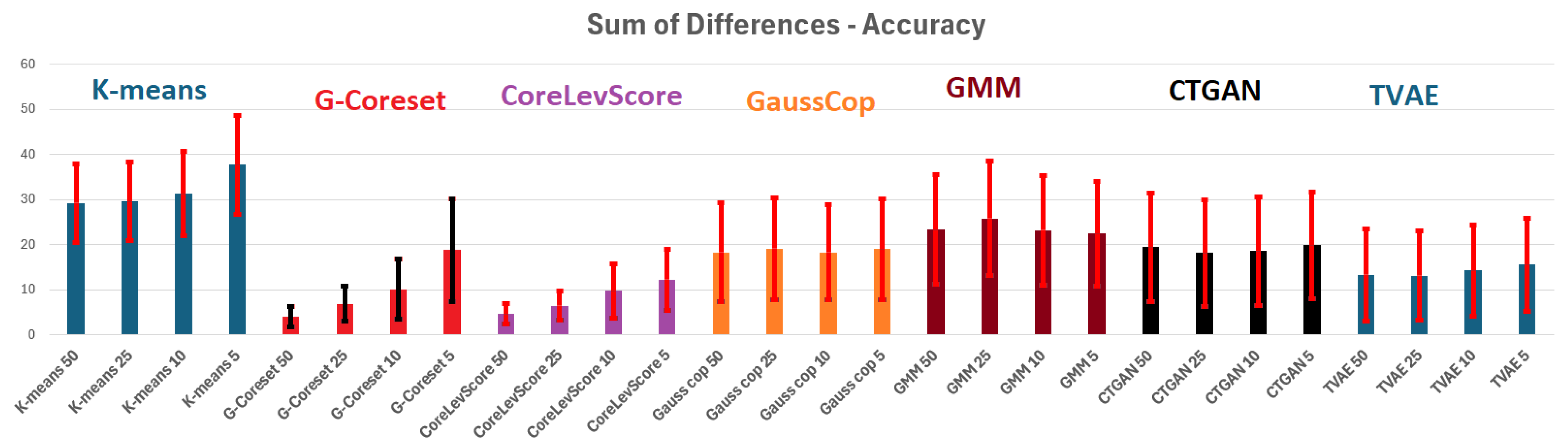
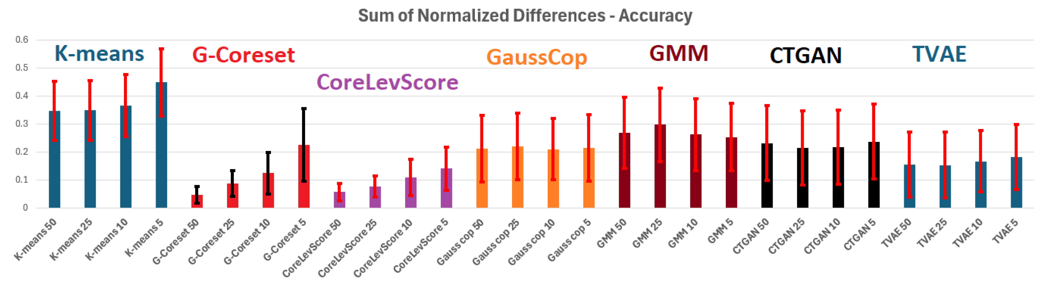
For classification, the aggregated SD and SND values, with respect to accuracy as a metric, are visually shown in Figure 2 and Figure 3 and followed numerically in

Table 10. Sum of differences (SD) between baseline and distilled accuracy (measured in [%]) with respect to the distillation method and percentage of cardinal of the distilled database w.r.t the original. Smaller values are better.

Percent.	K-Means	G-Coreset	CoreLevSc	GaussCop	GMM	CTGAN	TVAE
50	29.19	3.99	4.63	18.26	23.33	19.47	13.33
25	29.58	6.90	6.43	19.08	25.83	18.12	13.10
10	31.26	10.12	9.79	18.26	23.16	18.55	14.28
5	37.68	18.78	12.25	18.97	22.415	19.83	15.57
Average	31.92	9.95	8.28	18.64	23.69	18.99	14.07

and

Table 11. Sum of normalized differences (SND) between baseline and distilled accuracy with respect to the distillation method and percentage of cardinal of the distilled database w.r.t the original. Smaller values are better.

Percentage	K-Means	G-Coreset	CoreLevSc	GaussCop	GMM	CTGAN	TVAE
50	0.348	0.049	0.059	0.212	0.270	0.233	0.157
25	0.350	0.087	0.077	0.221	0.298	0.215	0.154
10	0.366	0.125	0.110	0.211	0.263	0.218	0.167
5	0.449	0.226	0.141	0.215	0.254	0.238	0.183
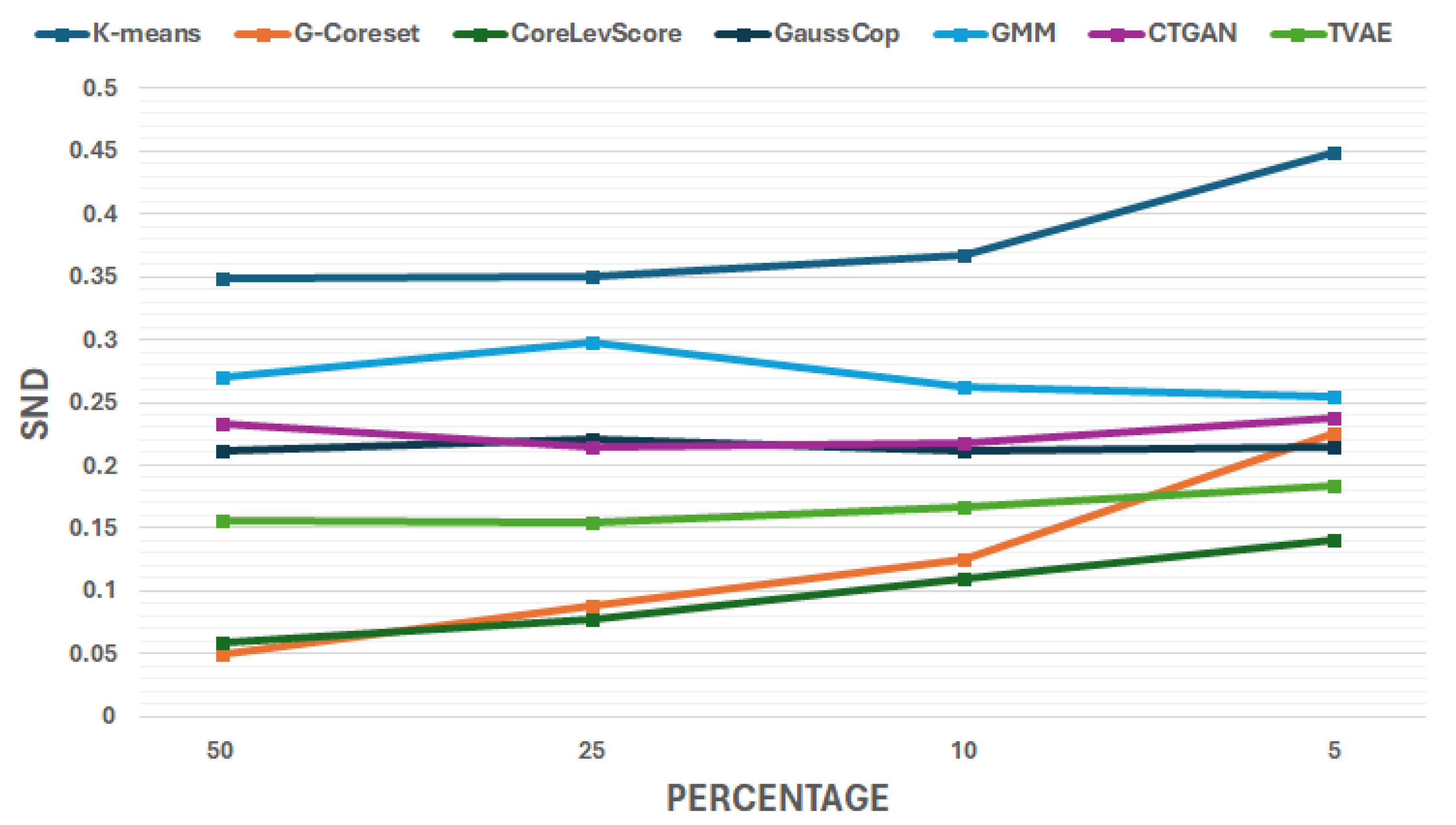
Average	0.378	0.122	0.097	0.215	0.271	0.226	0.165

. To better show the trends while doing distillation, we plot the SND variation with respect to the percentage in Figure 4.

For the Average Accuracy, the results are in

Table 12. Sum of differences (SD) between baseline and distilled Average Accuracy with respect to the distillation method and percentage of cardinal of the distilled database w.r.t the original. Smaller values are better.

Percentage	K-Means	G-Coreset	CoreLevSc	GaussCop	GMM	CTGAN	TVAE
50	18.19	7.42	8.54	24.45	30.68	22.16	20.31
25	18.46	10.33	11.32	24.92	32.04	22.13	18.47
10	20.72	14.82	17.24	24.91	30.32	23.45	21.51
5	24.41	23.71	20.23	26.81	30.62	21.92	23.42
Average	20.42	14.01	14.37	25.28	30.96	22.46	20.92

and

Table 13. Sum of normalized differences (SND) between baseline and distilled Average Accuracy with respect to the distillation method and percentage of cardinal of the distilled database w.r.t the original. Smaller values are better.

Percentage	K-Means	G-Coreset	CoreLevSc	GaussCop	GMM	CTGAN	TVAE
50	23.83	10.82	12.48	32.03	38.64	29.65	27.36
25	23.44	14.83	15.53	32.45	40.05	29.23	24.43
10	26.27	20.03	22.64	32.32	37.78	30.13	27.92
5	30.52	30.22	26.29	34.64	38.43	28.96	30.92
Average	26.03	19.06	19.22	32.84	38.73	29.45	27.66

.

When analyzing the results, several conclusions stand out:

• All distillation methods lose performance. The minimal loss starts at about 4% in accuracy when the dataset is reduced by half and increases to roughly 12.5% when the distilled dataset is only 5% of the full dataset. In some specific cases (i.e., particular datasets), there is a performance increase after distillation, but these cases are rare and likely incidental.
• The behavior of the distillation methods is consistent across variations, whether with respect to the dataset, the learner used, or the evaluation metric. This consistency refers both to the magnitude of performance loss and to the relative ranking with respect to classifiers; these aspects can be examined in more detail in the raw results provided in the Supplementary Materials.
• The best-performing methods are clearly the coreset-based approaches. While the method based on the Gonzalez algorithm performs better when the reduction is moderate (e.g., to 50%), the overall best performer is the Leverage Score-based coreset, which preserves much of the performance even under more aggressive reductions. When considering Average Accuracy, the G-coreset emerges as a clearer winner.
• On the opposite end, K-means is by far the worst performer. This is easily explained by the fact that the method is designed to capture cluster means rather than decision boundaries, which are critical for classification. Based on this finding, we do not further evaluate the K-means algorithm.
• The Gaussian-based generative methods (Gaussian Copula Synthesizer and Gaussian Mixture Models) generally perform poorly when compared to the coreset methods.
• Among the two modern neural network-based methods, TVAE surprisingly performs better. This is somewhat unexpected, since in the original work [16], the main proposal was CTGAN.
• When comparing results based on accuracy and Average Accuracy, the overall trends are consistent. The main difference is that the numerical values for Average Accuracy are lower and the performance loss due to distillation is larger. One may hope that supervised distillation, where class labels are used, may lead to more balanced results on Average Accuracy.
• When distilling moderately, all methods lead to decent results. Coreset methods produced good results no matter the problem.
• When distilling aggressively (to 5%), on specific databases, even the best method fails (i.e., performance is random change, or learner not converging). This suggests that success with aggressive distillation ratios is problem-dependent.
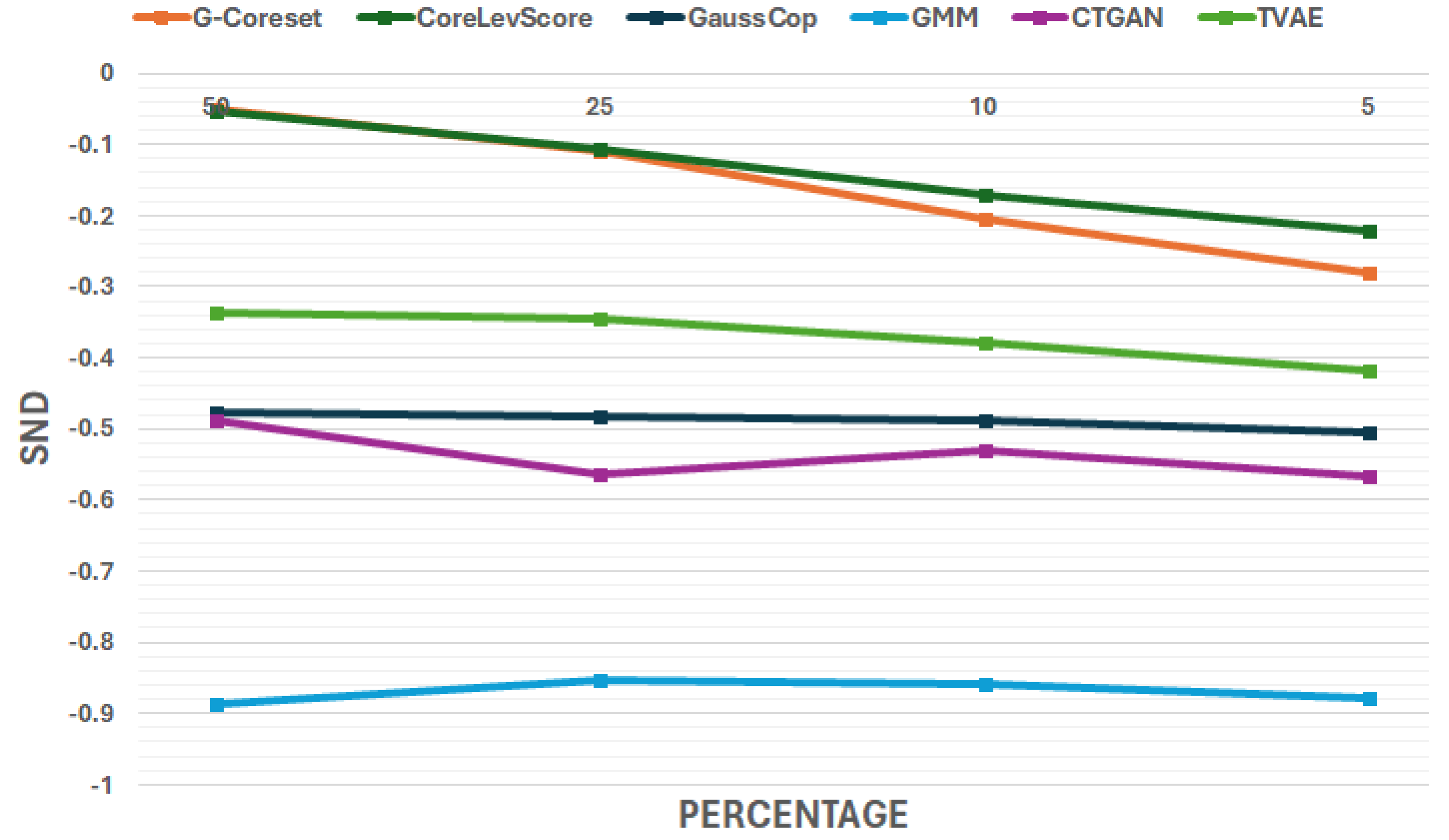
• While some distillation methods lose performance more rapidly (e.g., G-Coreset), others, such as CTGAN, maintain nearly constant performance. However, this observation is of limited relevance because the predicted crossing point occurs at a value below zero, which is not feasible.

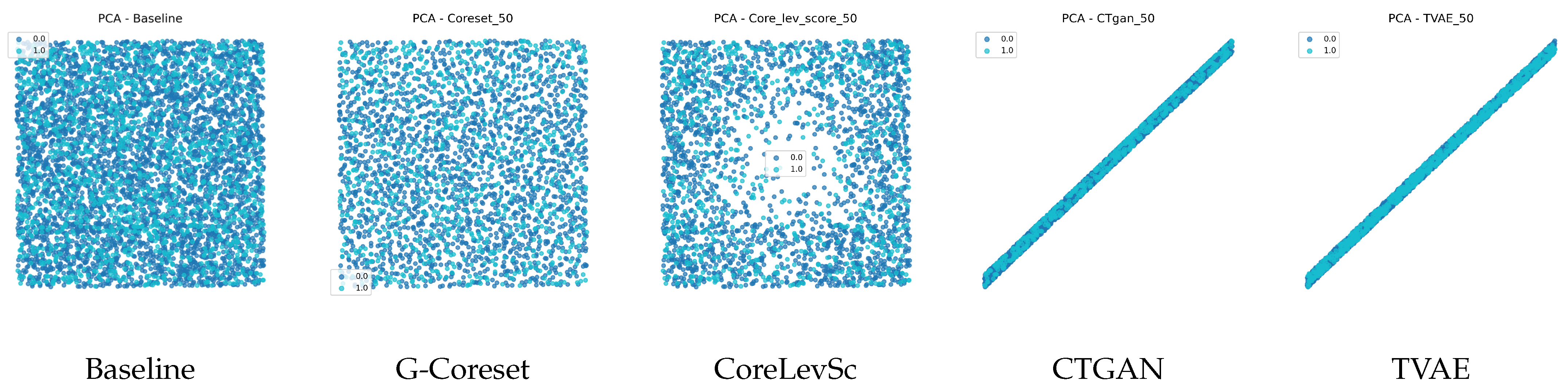
To further look into the behavior of the methods, we use visualization. While more plots are in provided in Figures S1–S4 from the Supplementary Materials, here we present some that are more informative. In Figure 5, we represent the original set and the distilled versions with G-Coreset ones CTGAN and TVAE. We recall that PCA ensures geometric comparability, but may miss non-linear complex structures. Note in the figure how coreset methods, especially CoreLeverageScore, preserve the space of the original dataset, while CTGAN and TVAE dramatically compress it.

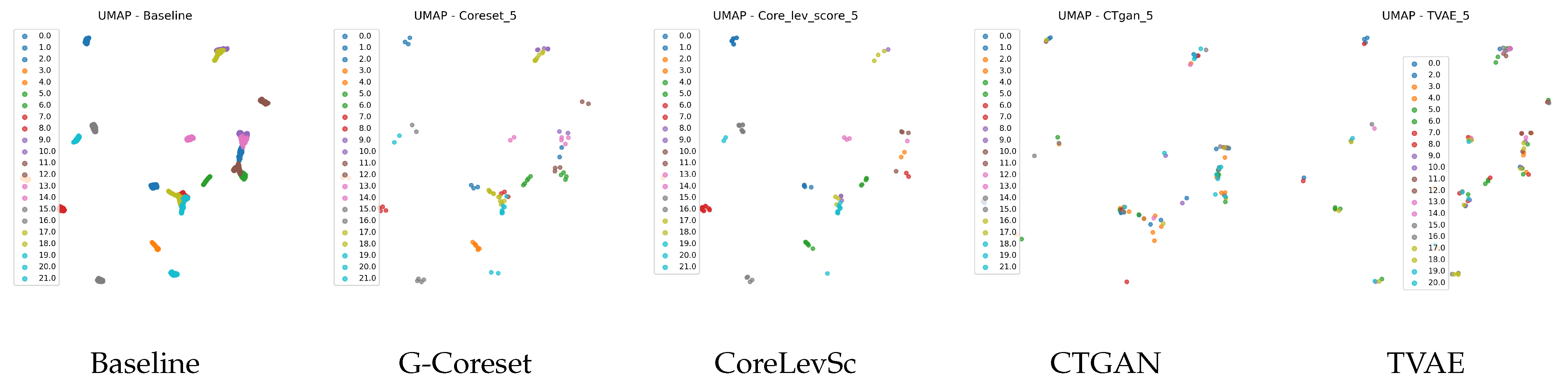
For a complementary view, we present in Figure 6 UMAP visualization of Crop Recommendation methods. We recall that UMAP is built to inspect non-linear manifold preservation. One may observe that the structures exiting in the original dataset, despite dramatic reduction, are clearly preserved by the coreset methods, while the neural methods lead to less clear separation.

Correlation with Tailness. Here we try to answer to the question: Can we use a taillness metric to predict the behavior of distillation methods?

To answer this question, we compute the correlation coefficient between the considered tailness measures and difference between the accuracy on the baseline and the accuracy on the distillation set, while varying the databases. An absolute value close to 1 would signal that a specific tailness measure is a very good indicator of the distillation method behavior, while values closer to zero mean that there is no indication.

The results are shown in

Table 14. Correlation between the loss in accuracy and four tailness measures while aggregated over all databases and over all percentages of distillation reductions. Absolute values closer to 1 are better.

Distillation	MeanAbsSkew	MeanExKurt	MeanTailRat99-01	MultivTail Frac
G-Coreset	−0.046	−0.148	−0.501	0.269
CoreLevSc	−0.054	−0.129	−0.437	0.323
CTGAN	−0.089	−0.158	−0.472	0.156
TVAE	−0.096	−0.149	−0.476	0.119

. As one may notice, the only relevant connection is with respect to MeanTailRatio99-01, where absolute values near 0.5 indicate a medium correlation. The negative values mean anti-correlation: the MeanTailRatio value is larger and the decrease (which is aimed) in accuracy of the distillation metrics is smaller. Thus, databases with larger tails are better summarized by distillation methods. Another point is a rather notable difference between the two coreset methods; here our finding is negative—the best performing method, Coreset Leverage Score, is poorly anticipated by the tailness metric.

We further investigate if the MeanTailRatio99-01 is better related to a specific distillation case (i.e., when the reduction is 50%, 25%, 10%, or 5%). The results are in

Table 15. Correlation between the loss in accuracy and the MeanTailRat99-01 tailness measure (aggregated over all databases) w.r.t percentages of distillation reductions. Absolute values closer to 1 are better.

Distillation	50%	25%	10%	5%
G-Coreset	0.169	−0.344	−0.358	−0.641
CoreLevSc	−0.204	−0.441	−0.438	−0.426
CTGAN	−0.479	−0.495	−0.338	−0.544
TVAE	−0.448	−0.490	−0.474	−0.469

. The results are rather uniform with the exception of the G-Coreset method, where the correlation significantly increases.

6.7.2. Regression

The full, raw results for the regression problems are in Tables S30–S53 in the Supplementary Materials. Here we present the aggregated results.

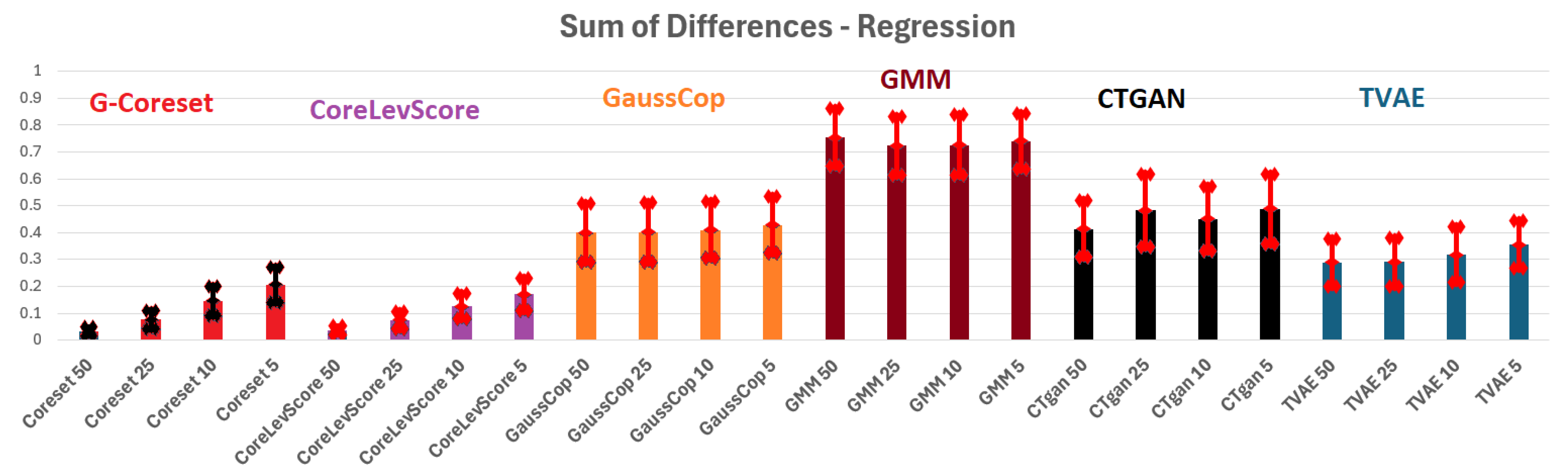
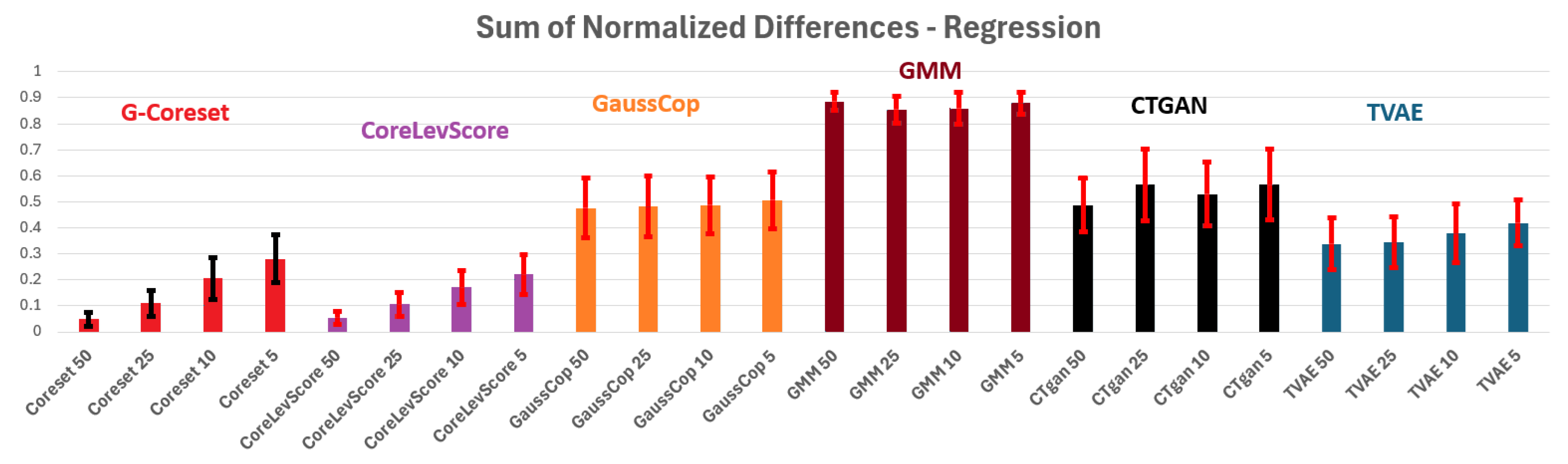
For aggregating the regression results, we used the same measures as in the case of classification, namely sum of differences (SD) and sum of normalized differences (SND). Compared to classification, this time, the measures are aggregating Mean Square Errors and, respectively, Pearson Correlation Coefficient. An additional change is that, due to poor results on classification, we have stopped evaluating K-means as a distillation method.

For regression, the aggregated SD and SND values, with respect to MSE as metric, are in

Table 16. Sum of differences (SD) (scaled with $\dot{1}{0}^5$) between baseline and distilled MSE with respect to the distillation method and percentage of cardinal of the distilled database w.r.t the original. Smaller values are better.

Distillation	G-Coreset	CoreLevSc	GaussCop	GMM	CTGAN	TVAE
50	5.733	9.774	99.597	210.169	165.598	77.586
25	16.223	19.305	103.557	187.739	204.299	61.127
10	31.487	26.378	120.256	194.128	215.105	82.606
5	59.436	40.704	131.681	209.649	211.956	160.287
Average	28.220	24.040	113.773	200.421	199.239	95.402

and

Table 17. Sum of normalized differences (SND) between baseline and distilled MSE with respect to the distillation method and percentage of cardinal of the distilled database w.r.t the original. Smaller values are better.

Distillation	G-Coreset	CoreLevSc	GaussCop	GMM	CTGAN	TVAE
50	0.352	0.420	10.799	28.205	10.170	6.834
25	1.058	1.181	10.477	27.888	9.638	7.243
10	3.018	2.429	11.039	28.003	9.764	8.567
5	4.424	3.496	10.803	26.858	10.531	9.052
Average	2.213	1.881	10.780	27.739	10.026	7.924

, while w.r.t Pearson Correlation are in

Table 18. Sum of differences (SD) between baseline and distilled Pearson Correlation Coefficient with respect to the distillation method and percentage of cardinal of the distilled database w.r.t the original. Smaller values are better.

Distillation	G-Coreset	CoreLevSc	GaussCop	GMM	CTGAN	TVAE
50	0.032	0.036	0.400	0.754	0.414	0.289
25	0.076	0.074	0.402	0.723	0.482	0.290
10	0.146	0.127	0.410	0.727	0.451	0.317
5	0.206	0.171	0.429	0.740	0.489	0.356
Average	0.115	0.102	0.410	0.736	0.459	0.313

and

Table 19. Sum of normalized differences (SND) between baseline and distilled Pearson Correlation Coefficient with respect to the distillation method and percentage of cardinal of the distilled database w.r.t the original. Smaller values are better.

Distillation	G-Coreset	CoreLevSc	GaussCop	GMM	CTGAN	TVAE
50	0.049	0.054	0.476	0.886	0.487	0.338
25	0.111	0.105	0.482	0.854	0.565	0.345
10	0.206	0.171	0.487	0.860	0.529	0.379
5	0.281	0.220	0.506	0.880	0.566	0.419
Average	0.162	0.138	0.488	0.870	0.537	0.370

. A graphical representation for the latter is shown in Figure 7 and Figure 8. The trends for each distillation method are provided in Figure 9.

Analyzing the results, similar conclusions to the experiments for classification can be drawn. Yet there are some particular notes:

• Distillation methods, in general, lose performance in the regression tasks too. This, in terms of correlation, ranges from $0.032$ when considering half the database to approximately $0.132$ when considering a set of only 5% of the original set size.
• The loss is more abrupt for G-Coreset than for CTGAN, but this does not compensate for possible (i.e., given by a positive number) reduction.
• Again the best performing methods are, clearly, the coreset methods, with a similar edge at large sets for G-Coreset; the overall best is the coreset based on Leverage Score.
• On the opposite side, with the K-means discounted, the worse are, again, Gaussian-based generative methods.
• Again, TVAE is better than CTGAN. Yet once more, it is not a tight competitor for coreset methods.
• A particularly interesting aspect in the regression setting is the difference between the findings when performance is measured using MSE versus correlation, as well as between non-normalized and normalized metrics. In terms of raw MSE, distillation significantly increases the loss in performance. However, after normalization, the loss appears relatively small. This suggests that distillation methods introduce a significant bias in the predictions; however, they still capture the overall trend well, as indicated by the correlation-based measures.

6.8. Do Distillation Methods Change the Nature of the Dataset?

To evaluate this aspect, we look at the performance variation while doing a hyperparameter search on the dataset, with the standard deviation as the metric. The raw results are in the Supplementary Materials in Tables S54–S57. The aggregated results for the XGBoost (best learner) classification are in

Table 20. Average overall standard deviation over accuracies obtained with XGBoost while doing hyperparameter search in classification. The baseline (without distillation) value is 0.0176. Better values are smaller.

Distillation	K-Means	G-Coreset	CoreLevSc	GaussCop	GMM	CTGAN	TVAE
50	0.090	0.134	0.133	0.112	0.104	0.107	0.122
25	0.089	0.129	0.129	0.112	0.100	0.109	0.121
10	0.086	0.126	0.126	0.114	0.105	0.116	0.117
5	0.075	0.110	0.127	0.119	0.114	0.113	0.121
Average	0.085	0.125	0.129	0.114	0.106	0.111	0.120

.

As one might see, with the exception of K-means, all other distillation methods dramatically increased the range of accuracies, signaling that the smaller dataset becomes less and less consistent. While this is expected, it also means that the same set of hyperparameters that lead to the best value is no longer automatically viable when learning a distilled set.

Another observation, this time more intriguing, is the deviation, while larger than the baseline, it is almost constant or even decreasing while reducing the training set. This means that the distillation method changes the structures of the points (in a way not captured by Wasserstein distance), but does it in a consistent way: the nature of the distillation matters more and not the percentage of reducing.

7. Duration

A key aspect of the distillation is the reduction of the training time. For this experiment, we used a single CPU (Intel(R) Core(TM) i5-13400F—10 cores, 16 threads, 4.60 Ghz) running Python 3.10.12. Full and detailed results are in the Supplementary Materials in Tables S58–S61. Averaged data (over all classification datasets) is shown in

Table 21. Averaged duration [s] over all classification datasets, with respect to percentage. The best values are marked with bold.

Distillation	K-Means	G-Coreset	CoreLevSc	GaussCop	GMM	CTGAN	TVAE
50	105.457	204.832	0.057	20.275	12.760	226.124	150.840
15	49.078	102.317	0.056	25.757	11.876	230.374	148.718
10	21.092	41.049	0.054	25.162	11.171	227.562	146.581
5	9.527	20.573	0.038	25.263	10.990	229.780	144.551
Average	46.288	92.193	0.051	24.114	11.699	228.460	147.673

.

We recall that while theoretically CTGAN and TVAE might use GPU, their creators advocate against it, so in this evaluation, they have not been used. All processing here is CPU-only, single thread (no parallelization).

The results presented here should be interpreted as relative indications rather than absolute evaluations. Parallelization and further optimization could reduce the reported runtimes. From the data, it can be observed that the most efficient method by far is the Coreset Leverage Score approach. K-means is faster in terms of runtime, but its poor performance outweighs this advantage. Neural network-based methods require significantly longer execution times.

The G-Coreset method in general require a short runtime. The average is pushed high by the duration on Credit Card Fraud, where to compute the 50% distillation set, an astounding 3061 s was needed, which questions the usability of the method, in this implementation, on large datasets. If the results on this database would be ignored, then G-Coreset would rank second behind Coreset Leverage Score.

In general, most methods exhibit relatively constant runtimes regardless of the distillation percentage. This is because they first construct a representation of the original dataset, which is the most computationally intensive step, and then perform sampling, which accounts for only a small fraction of the total runtime. A notable exception is G-Coreset, which computes each point in the distilled set independently and therefore scales linearly with the size of the distilled dataset; G-Coreset also scales upward with dimensionality; in contrast, Coreset Leverage Score uses PCA to set dimensionality at a fixed size, and thus is near-independent to the database dimensionality.

Regarding specific results, the runtime of all distillation methods on the Credit Card Fraud dataset is significantly higher, as this dataset is larger both in terms of the number of instances and feature dimensionality. Consequently, for all methods, the runtime on this dataset appears as an upper-end outlier.

8. Discussion and Limitations

8.1. Relation with Prior Findings

Two main paradigms have emerged for dataset compression: synthetic data generation and instance selection (coresets). Coreset selection predates modern dataset distillation and has long been studied as a principled method for approximating large datasets with representative subsets. Indeed, dataset distillation itself is often presented as a successor to earlier coreset approaches [74].

In contrast, much of the recent tabular synthesis literature focuses on generative approaches (e.g., GAN-based or diffusion-based models) [3,75], typically evaluated on a small number of datasets and often without including classical instance selection baselines [16,17]. At the same time, surveys of dataset compression still identify coreset selection as a fundamental technique for reducing training data while preserving predictive performance.

Our work aims precisely to bridge these two lines of research. By evaluating both generative methods and instance selection approaches across a large set of classification and regression tasks, we provide a broad empirical comparison that has been largely missing from prior work. Our results indicate that, for tabular data and the downstream predictive tasks considered, classical coreset methods remain highly competitive and outperform synthetic generators.

One possible explanation is that tabular datasets frequently involve heterogeneous feature types and non-differentiable learners such as tree ensembles [20], which complicates the optimization of synthetic datasets and may favor methods that directly preserve the empirical data geometry.

8.2. Theoretical Support

In short, the findings of this paper argue that coreset (instance-based selection) are more suitable for distillation if the ranking criteria is downstream prediction accuracy under supervised learning.

First let us note that instance selection approximates the original empirical distribution:

$${\hat{P}}_n={\displaystyle \frac{1}{n}}\sum _{\mathbf{x}\in \mathcal{X}}{\delta }_{{\mathbf{x}}_i}\approx {\displaystyle \frac{1}{k}}\sum _{\mathbf{x}\in \mathcal{S}\subset \mathcal{X}}{\delta }_{{\mathbf{x}}_i}$$

(35)

Generators approximate the true distribution $P\left(\mathcal{D}\right)$. This approximation assumes some underlying model by which the actual samples ${\mathbf{x}}_i$ are drawn from the true data $\mathcal{D}$. The generators aim to invert this model, which is an assumption. Since the test is based on real data, one might argue that instance selection is more suitable.

A similar rationale may be constructed for the downstream supervised evaluation. For supervised learning, coreset methods approximate the empirical sum (in the loss function) directly:

$${\displaystyle \frac{1}{N}}\sum _{\mathbf{x}\in \mathcal{X}}\ell (f\left({\mathbf{x}}_i\right),y_i)\approx {\displaystyle \frac{1}{k}}\sum _{\mathbf{x}\in \mathcal{S}\subset \mathcal{X}}\ell (f\left({\mathbf{x}}_i\right),y_i),$$

(36)

where $k\ll n$.

Generators approximate the expectation of the loss function ${\mathbb{E}}_{\mathbf{x}\sim P_{gen}}\ell (f\left(\mathbf{x}\right),y)$. However, if $P_{gen}\ne {\hat{P}}_{empirical}$, the risk landscape shifts. In finite-sample supervised settings, empirical-risk approximation may be superior, which matches the findings in this paper.

8.3. Limits of the Experiments

In this paper, we investigated seven distillation methods. All methods are unsupervised, in the sense that they do not use labels while condensing the dataset. The conclusions may differ if distillation explicitly takes labels into account. In other words, during distribution matching, we only match $P\left(\mathcal{X}\right)$ and subsequently obtain $P\left(\mathcal{Y}\right)$ from the data. A joint optimization over $P(\mathcal{X},\mathcal{Y})$ may, therefore, lead to different conclusions.

The self-imposed restriction of investigating distillation methods independently of the learner lead to the exclusion of popular methods such as those based on gradient matching [13] or Trajectory Matching [76]. They are powerful classes of methods, but inherently connect the distillation set to a learner trained by back-propagation.

Our conclusions primarily apply to tabular datasets of medium-to-large dimensionality and to classical machine learning learners (Random Forest, Support Vector Machine, XGBoost). Although the observed superiority of coreset methods holds consistently across all experiments and compression levels tested, we do not implicitly extend this conclusion to neural tabular models. Performance trends may differ for very-high-dimensional data or for end-to-end deep learning pipelines. We investigated both classification and regression tasks, but not clustering (explicitly), retrieval, or representation learning.

While we performed hyperparameter searches for each learner, the search ranges were limited and the learners were used largely in an off-the-shelf manner. We did not pursue extensive fine-tuning for each classifier. Nevertheless, we showed that our baseline performance is comparable to prior studies. More careful and intensive tuning may lead to slightly different results.

All methods presented in the main paper are feasible even for larger datasets. Most scale linearly with respect to the number of instances N. In the Supplementary Materials, we also discuss another method, namely Coreset Facility Location Submodular Optimization, which—despite being a strong performer—has quadratic memory requirements. This makes it impractical for large-scale datasets and conflicts with the core motivation of data distillation.

The relative ranking of distillation methods (for a specific dataset and reduction ratio) is influenced by the choice of the learner, suggesting that no single method is universally optimal. Nevertheless, coreset-based methods performed best in the vast majority of the cases studied.

Another limitation concerns the evaluation metrics. For classification, we used accuracy and Average (Balanced) Accuracy, while for regression, we used Mean Squared Error and the Pearson Correlation Coefficient. We did not consider task-specific metrics such as the F1-score, Area Under the Curve, or ranking-based metrics. Again, our evaluation focuses primarily on downstream predictive performance.

We also investigated some desirable properties, such as interpretability, by means of visualization and correlations with tailness metrics. Our findings are restricted to the techniques used, namely PCA, t-SNE, and UMAP for visualization, and the four tailness metrics considered. Other methods or metrics may lead to slightly different conclusions.

8.4. Stability

The reported results, being averaged over many datasets, are stable. Core experiments (best learner for each case) were repeated five times, and the aggregated results show virtually no change.

Variability appears when considering a specific learner (defined by the model and precise hyperparameter values) applied across consecutive runs of a distillation method. However, similar performance can typically be recovered through slight adjustments (i.e., tuning) of hyperparameters. Variability is somewhat larger for very aggressive distillation ratios, but even in these cases, the hyperparameter search is generally able to compensate. Overall, the aggregated results are very stable.

8.5. Efficiency Trade-Off

Distillation inevitably trades accuracy for efficiency. When averaged over multiple datasets, all distillation methods lead to some loss in performance.

In general, moderate reductions of the training dataset (e.g., to 50%) incur limited performance loss (approximately 3–5% in accuracy or about 0.03 in correlation). This can be partially attributed to the relatively large size of the original datasets, which makes moderate distillation less harmful.

In contrast, aggressive distillation leads, in an increasing number of cases, to a steeper degradation in performance, indicating a practical lower bound on dataset size for reliable learning. This bound is highly dataset-dependent. For example, when distilling to 5% of the data, accuracy losses for XGBoost with Leverage Score-based coresets ranged from minimal (e.g., a 3% accuracy loss) to nearly complete failure to learn (e.g., on the Crop Recommendation or Red Wine datasets).

Overall, halving the dataset size is reliable regardless of the method used, whereas stronger distillation ratios are both method- and dataset-dependent. Among the evaluated approaches, G-Coreset proved to be the most stable.

9. Conclusions

In this paper, we evaluated seven unsupervised distillation methods across 17 classification and nine regression tasks. Distillation was assessed in terms of downstream predictive performance using off-the-shelf learners such as Random Forest, Support Vector Machine, and XGBoost.

This work does not propose new distillation algorithms; instead, it provides a systematic empirical evaluation of existing methods within a unified experimental framework. The investigation was conducted in a structured and disciplined manner: dataset reductions were performed at fixed and meaningful percentages, and while the learners were moderately tuned, the tuning process was applied consistently across all experiments.

We found coreset-based methods to be the most reliable from multiple perspectives, including both predictive performance and computational efficiency. More recent neural network-based methods were, somewhat surprisingly, found to be inferior in this setting. Among the coreset approaches, the Leverage Score-based coreset emerged as a robust all-around solution, while G-Coreset was able to achieve better performance under low distillation ratios, albeit with occasionally high runtimes.

We also investigated the correlation between distillation performance and dataset tailness and found that the proportion of outliers is moderately anti-correlated with performance across all methods, with a stronger effect observed for coreset-based approaches. This suggests that precomputing the outlier ratio may help form expectations regarding distillation success.

Finally, we examined dataset-level learning consistency by measuring the variation in learner predictive performance with respect to hyperparameter changes. Distillation to smaller dataset sizes does introduce some variation, as the variance increases by, roughly, a factor of 10.

Lastly, we contribute to the community by making our code fully public, enabling others to reproduce and extend our experiments.