
Article

Explainable Kolmogorov–Arnold Networks for Zero-Shot Human Activity Recognition on TinyML Edge Devices


1
Multidisciplinary Faculty of Nador, Mohammed Premier University, Oujda 60000, Morocco
2
Laboratory LaSTI, ENSAK, Sultan Moulay Slimane University, Khouribga 54000, Morocco
*
Author to whom correspondence should be addressed.
Mach. Learn. Knowl. Extr. 2026, 8(3), 55; https://doi.org/10.3390/make8030055
Submission received: 1 January 2026 / Revised: 2 February 2026 / Accepted: 11 February 2026 / Published: 26 February 2026
(This article belongs to the Section Learning)

Abstract

Human Activity Recognition (HAR) on wearable and IoT devices must jointly satisfy four requirements: high accuracy, the ability to recognize previously unseen activities, strict memory and latency constraints, and interpretable decisions. In this work, we address all four by introducing an explainable Kolmogorov–Arnold Network for Human Activity Recognition (TinyKAN-HAR) with a zero-shot learning (ZSL) module, designed specifically for TinyML edge devices. The proposed KAN replaces fixed activation functions by learnable one-dimensional spline operators applied after linear mixing, yielding compact yet expressive feature extractors whose internal nonlinearities can be directly visualized. On top of the KAN latent space, we learn a semantic projection and cosine-based compatibility function that align sensor features with class-level semantic embeddings, enabling both pure and generalized zero-shot recognition of unseen activities. We evaluate our method on three benchmark datasets (UCI HAR, WISDM, PAMAP2) under subject-disjoint and zero-shot splits. TinyKAN-HAR consistently achieves over 97% macro-F1 on seen classes and over 96% accuracy on unseen activities, with harmonic mean above 96% in the generalized ZSL setting, outperforming CNN, LSTM and Transformer-based ZSL baselines. For explainability, we combine gradient-based attributions, SHAP-style global relevance scores and inspection of the learned spline functions to provide sensor-level, temporal and neuron-level insights into each prediction. After 8-bit quantization and TinyML-oriented optimizations, the deployed model occupies only 145 kB of flash and 26 kB of RAM, and achieves an average inference latency of 4.1 ms (about 0.32 mJ per window) on a Cortex-M4F-class microcontroller, while preserving accuracy within 0.2% of the full-precision model. These results demonstrate that explainable, zero-shot HAR with near state-of-the-art accuracy is feasible on severely resource-constrained TinyML edge devices.

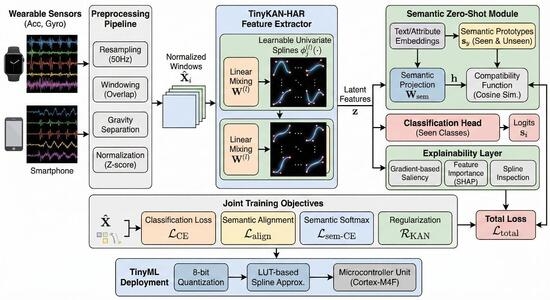
Graphical Abstract

1. Introduction

Human Activity Recognition [1] from wearable and mobile sensors has become a key enabling technology for a wide range of applications, including health and fitness monitoring, rehabilitation, smart homes, industrial safety, and context-aware human–computer interaction [2]. Recent advances in inertial measurement units (IMUs), low-power wireless communication, and embedded processors have made it possible to continuously collect rich multivariate time-series data from accelerometers, gyroscopes, and other sensors [3]. Translating these raw signals into reliable activity labels on-device is essential for building responsive, privacy-preserving, and energy-efficient systems that can operate without permanent cloud connectivity.
Despite the rapid progress of deep learning in HAR, several important challenges remain. First, deployed systems must achieve high recognition accuracy under realistic conditions, including subject variability, sensor placement changes, and noisy measurements [4]. Second, real-world deployments frequently encounter activities that were not present during training, for example new exercise routines, novel gestures, or unforeseen occupational tasks. Conventional supervised learning pipelines are not designed to recognize such unseen classes and therefore tend to misclassify them as the most similar known activity, which can be problematic in safety-critical scenarios [5]. Third, many emerging applications operate under strict resource constraints: wearable devices and IoT nodes often rely on microcontrollers with a few hundred kilobytes of flash, tens of kilobytes of RAM, and milliwatt-level power budgets. Finally, there is a growing demand for models whose predictions can be interpreted and trusted by domain experts, clinicians, and end-users, especially when decisions are used to trigger interventions or are recorded in medical or occupational records [6]. Deep neural networks based on convolutional neural networks (CNNs), recurrent neural networks (RNNs), and Transformer architectures have achieved impressive performance on benchmark HAR datasets [7,8]. However, these models are typically over-parameterized for deployment on resource-constrained microcontrollers, often requiring hardware accelerators or offloading to the cloud [9]. Moreover, their decision process is usually opaque, as the learned internal representations are difficult to relate to physically meaningful patterns in the sensor signals. Although post-hoc explanation methods such as saliency maps, gradient-based relevance scores, and Shapley-value approximations have been applied to time-series models, the resulting explanations can be unstable and are not always aligned with the underlying model structure [10]. In parallel, TinyML research has proposed compressed and quantized models tailored for microcontrollers, yet most of these efforts have prioritized footprint and latency over explainability and the ability to handle unseen activities [11]. Zero-shot learning (ZSL) offers a principled way to recognize unseen classes by leveraging auxiliary semantic information such as textual descriptions, attributes, or embeddings derived from large language models [12,13]. In the ZSL paradigm, the model learns a compatibility function between input features and semantic class prototypes, allowing it to infer labels for classes that were not present in the training set but whose semantic representations are available at test time [14]. While ZSL has been widely studied in computer vision and, to a lesser extent, in audio and generic time series, its application to HAR remains relatively unexplored [15], especially under microcontroller-level resource constraints. Existing ZSL approaches typically rely on high-capacity backbones and are not designed for quantized TinyML deployment, nor do they explicitly address interpretability [16].
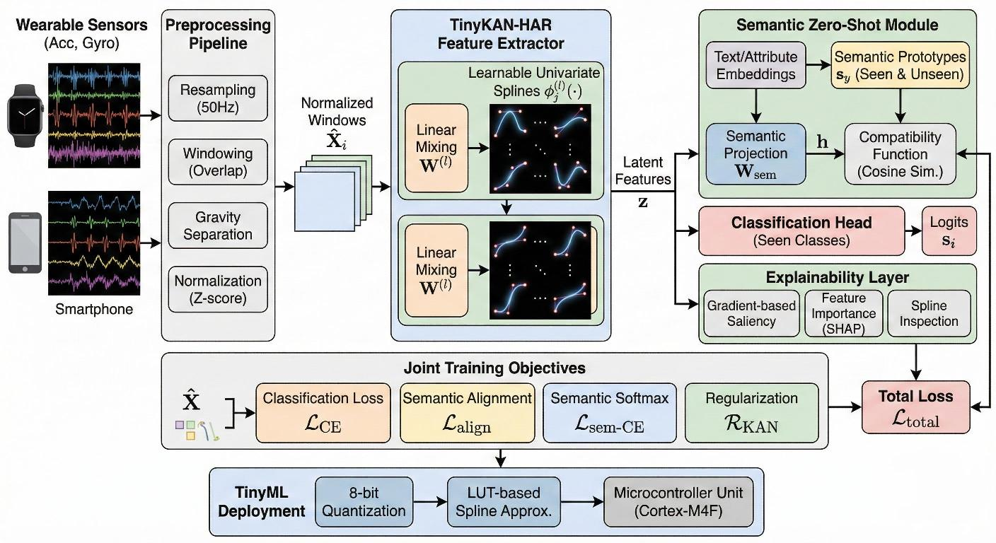
In this work, we tackle these challenges by combining three complementary ideas: (1) compact yet expressive neural architectures suitable for TinyML deployment, (2) semantic-embedding-based zero-shot learning tailored to sensor-based HAR, and (3) intrinsic and post-hoc explainability mechanisms that provide multi-level insight into model decisions. Our starting point is the recently proposed Kolmogorov–Arnold Networks (KANs), which replace conventional pointwise activation functions with learnable one-dimensional spline operators applied after linear mixing. Compared to standard multilayer perceptrons, KANs can obtain similar or better accuracy with fewer parameters while exposing interpretable univariate nonlinearities that can be directly inspected. These properties make KANs an attractive candidate for building HAR models that are both compact and interpretable.
To make the model behavior transparent, we integrate several explainability mechanisms. At the input level, we employ gradient-based attribution methods to highlight which sensors and time steps have the strongest influence on the predicted activity, allowing practitioners to verify that the model focuses on meaningful motion patterns. At the feature level, we compute SHAP-style global relevance scores over the latent dimensions to identify the most important learned features for each class. At the neuron level, we directly inspect and visualize the learned spline functions in the KAN layers, which reveal interpretable nonlinear transformations of intermediate features and provide insight into how the model separates different activities. In this work, we distinguish between interpretability and explainability, which are often used interchangeably in the literature. We follow the common view that interpretability refers to intrinsic model properties that are directly understandable by humans, such as transparent architectures or components whose behavior can be explicitly inspected. In contrast, explainability refers to post-hoc techniques that aim to explain the predictions of an otherwise complex or opaque model, for example through attribution, relevance, or sensitivity analysis. This distinction allows us to clearly position the proposed approach as combining both intrinsic interpretability, enabled by Kolmogorov–Arnold Networks, and post-hoc explainability methods applied at multiple levels of the model.
The main contributions of this paper are summarized as follows:
  • We introduce TinyKAN-HAR, a compact KAN-based HAR architecture specifically designed for deployment on resource-constrained TinyML platforms, leveraging learnable spline-based nonlinearities to achieve high accuracy with a small memory footprint.
  • We develop a semantic-embedding-based zero-shot learning module on top of the KAN latent space that aligns sensor representations with class-level semantic prototypes, enabling recognition of both seen and unseen activities in pure and generalized zero-shot settings while remaining compatible with TinyML deployment via model compression and quantization-aware training.
  • We propose a multi-level explainability framework and conduct comprehensive experiments and ablation studies, showing that TinyKAN-HAR provides competitive or superior performance compared to strong CNN/RNN/Transformer baselines, while offering inherently interpretable decisions and practical guidelines for building accurate, transparent, and ultra-efficient HAR models on edge devices.
The remainder of this paper is organized as follows. Section 2 reviews the existing literature on sensor-based human activity recognition, TinyML, and explainable deep models. Section 3 introduces the proposed TinyKAN-HAR architecture and its zero-shot and explainability modules, datasets, preprocessing pipeline. Section 4 describes the baselines, and implementation details. Section 5 reports the quantitative and qualitative evaluation of the proposed approach. Section 6 provides an in-depth discussion of the results, design choices, limitations, and deployment implications. Finally, Section 7 concludes the paper and outlines directions for future work.

2. Related Work

2.1. Human Activity Recognition

HAR aims to automatically identify physical activities from sensor data [17]. In ubiquitous and wearable computing, HAR mainly relies on accelerometers, gyroscopes, and magnetometers embedded in smartphones, smartwatches, fitness trackers, and dedicated wearables, sometimes complemented by ambient sensors (e.g., motion, pressure, environmental) in smart-home settings [7,18]. Classical HAR pipelines segment raw signals into fixed or adaptive windows, extract hand-crafted time/frequency features (e.g., mean, standard deviation, energy, entropy, dominant frequency), and feed them to traditional classifiers such as KNN, SVMs, random forests, or gradient-boosted trees [19,20,21,22,23]. While effective, this approach relies heavily on domain-specific feature engineering and is sensitive to changes in sensor placement, sampling rate, or population [6]. Deep learning replaces hand-crafted features with learned representations from raw or lightly processed signals [1,2,3,4]. CNNs capture local temporal patterns in inertial data [24,25,26], whereas RNNs (LSTMs, GRUs) focus on long-term temporal dependencies [27,28,29,30,31]. More recent TCN and Transformer-based architectures use dilated convolutions or self-attention to model longer-range dependencies and support parallelization [32,33,34,35,36,37,38]. However, these models are mostly designed for resource-rich platforms (e.g., GPUs, desktop CPUs) and rarely target highly constrained edge devices.

2.2. TinyML and Edge Deployment

Tiny machine learning (TinyML) focuses on deploying ML models directly on severely resource-limited devices such as MCUs and ultra-low-power SoCs [11]. Typical targets offer only tens to a few hundreds of kilobytes of RAM, limited flash, and modest clock frequencies, often powered by small batteries or energy harvesting [39]. Under these constraints, models must simultaneously satisfy strict memory, compute (e.g., MAC operations), and energy budgets, while maintaining acceptable accuracy [40]. To support deep learning in this regime, a variety of compression and optimization techniques have been proposed, including post-training and quantization-aware training to low precision, pruning, low-rank factorization, and compact architecture design [41,42]. Frameworks such as TensorFlow Lite for Microcontrollers and CMSIS-NN provide optimized kernels tailored to embedded hardware [43,44]. HAR is a natural TinyML use case, as many wearables and IoT devices already integrate inertial sensors and benefit from on-device inference for privacy, bandwidth reduction, and low latency [45]. Existing TinyML HAR systems typically use shallow CNNs, small RNNs with aggressive compression, or classical ML models implemented in fixed-point arithmetic. However, most works assume a closed set of activities and pay limited attention to generalization to unseen activities or to interpretability directly on device [11].

2.3. Kolmogorov–Arnold Networks (KANs)

KANs are a neural architecture inspired by the Kolmogorov–Arnold representation theorem, which states that any multivariate continuous function can be expressed as a composition of univariate continuous functions and addition operations [46]. Unlike MLPs, which rely on linear transformations followed by fixed pointwise nonlinearities (e.g., ReLU, tanh), KANs parameterize learnable univariate functions along the edges and use simple linear combinations at the nodes [47]. In practice, these univariate functions are often implemented as spline-based units or other smooth basis functions with learnable coefficients, so each edge represents a flexible scalar function and each neuron aggregates its inputs linearly. This design can increase expressive power per parameter and yields more interpretable internal representations, as the learned univariate functions can be directly visualized [48]. KANs have shown promising results on regression for tabular data, low-dimensional scientific computing, and, more recently, in vision and signal-processing tasks [49]. For resource-constrained HAR, KANs are appealing because their higher expressivity per parameter can enable smaller models, the spline-based functions provide a natural handle for interpretability, and their arithmetic (look-ups and linear combinations) can be implemented efficiently on MCUs, making them a plausible backbone for TinyML-based HAR [50].

2.4. Zero-Shot Learning for Activity Recognition

Zero-shot learning (ZSL) aims to recognize classes unseen during training by exploiting auxiliary semantic information relating seen and unseen classes [14]. Instead of mapping inputs directly to labels, ZSL methods learn an embedding or compatibility function between input space and a semantic space hosting both seen and unseen classes [51]. At test time, an input is assigned to the class whose semantic representation best matches the predicted embedding. Two main semantic spaces are common. Attribute-based ZSL uses manually defined or weakly supervised attributes describing high-level class properties (e.g., “uses upper body”, “high energy”, “indoor”) [52]. Embedding-based ZSL instead adopts distributed text-based representations (word2vec, GloVe, BERT-like embeddings) for class names or descriptions [53], and learns to project sensor data into that space. For HAR, ZSL is attractive because the activity space is effectively unbounded, and collecting labeled data for all activities under all conditions is infeasible. Prior work has leveraged attributes or word embeddings for unseen activity recognition [54], but faces challenges such as semantic domain shift, hubness in high-dimensional embeddings, and the difficulty of defining meaningful attributes for complex activities. Moreover, existing ZSL methods for HAR are typically designed for resource-rich platforms and rarely consider TinyML deployment constraints.

2.5. Explainable AI in HAR and TinyML

Explainable AI (XAI) [55] aims to clarify how and why models make predictions. In HAR, interpretability supports user trust, human-in-the-loop decision making (e.g., healthcare, industrial monitoring), and model debugging. Explanations are often categorized into local and global ones: local methods explain individual predictions (e.g., identifying influential time steps, sensors, or features), while global methods summarize overall model behavior or decision rules. Common local techniques include perturbation- or gradient-based feature importance, saliency maps over time and channels, and example-based explanations that highlight similar training samples (prototypes) [56]. Global explanations can be derived via rule extraction, surrogate decision trees, or inherently interpretable model designs. On TinyML devices, XAI is particularly challenging: post-hoc methods may require many forward passes, large prototype sets, or gradient computations that are expensive or unsupported for quantized, integer-only models [57]. Storing explanation artifacts (e.g., attribution maps, surrogates) can also exceed available memory. Consequently, most deployed HAR systems on MCUs either omit explicit explanations or offload explanation computation to the cloud, which may conflict with privacy and latency requirements. This motivates architectures and explanation strategies that are intrinsically lightweight and amenable to on-device computation.

3. Proposed Methodology

3.1. Datasets

We evaluate the proposed explainable Kolmogorov–Arnold Network for zero-shot human activity recognition on TinyML edge devices using three publicly available datasets: UCI Human Activity Recognition Using Smartphones (UCI HAR), WISDM Smartphone and Smartwatch Activity and Biometrics, and PAMAP2 Physical Activity Monitoring.

3.1.1. UCI HAR Dataset

The UCI HAR dataset [58] contains recordings from 30 volunteers (aged 19–48 years) wearing a single smartphone (Samsung Galaxy S II) attached to the waist while performing six activities: WALKING, WALKING_UPSTAIRS, WALKING_DOWNSTAIRS, SITTING, STANDING and LAYING. A triaxial accelerometer and triaxial gyroscope sample linear acceleration and angular velocity at 50 Hz, yielding a six-dimensional raw sensor stream. The dataset provides pre-segmented windows of 128 samples (2.56 s) with 50% overlap, each labeled by the majority activity. We follow the original subject-wise split, where 21 subjects (about 70%) are used for training and 9 for testing. From the 21 training subjects, we randomly select 4 subjects for validation and keep the remaining 17 for model training, ensuring that no subject appears in more than one subset. This setup allows us to evaluate generalization to unseen users. For the ZSL scenario, we partition the six activities into seen and unseen classes. We treat level activities as seen and stair-related activities as unseen: WALKING, SITTING, STANDING and LAYING are used as seen classes, while WALKING_UPSTAIRS and WALKING_DOWNSTAIRS are unseen and only appear at test time. This reflects a practical scenario in which an on-device model trained on common activities must later recognize related but previously unseen motions such as stair walking based on semantic relations.
Preprocessing follows the original protocol: removal of sensor bias, separation of body and gravity acceleration using a low-pass filter, and per-channel normalization to zero mean and unit variance. Normalization statistics are computed on the training set only and applied to validation and test sets to avoid information leakage.

3.1.2. WISDM Smartphone and Smartwatch Activity Dataset

The WISDM Smartphone and Smartwatch Activity and Biometrics dataset [59] extends the smartphone-only setting by instrumenting 51 volunteers with both a smartphone and a smartwatch. For each subject, a triaxial accelerometer and triaxial gyroscope are recorded on each device as the subject performs 18 activities of daily living for approximately three minutes per activity. All four sensor streams (phone accelerometer, phone gyroscope, watch accelerometer, watch gyroscope) are sampled at 20 Hz. Activities include common motions (e.g., walking, jogging, walking_upstairs, walking_downstairs, sitting, standing) as well as fine-grained daily actions such as typing, brushing_teeth and using_stairmaster. After synchronization and alignment of the four sensor channels, we represent each window as a multivariate time series of dimension 12 (three axes from each of the four sensors). Using windows of 200 samples (10 s at 20 Hz) with 50% overlap, we generate time-series segments labeled with one of the 18 activities and associated with a subject identifier in { 1 , , 51 } . To obtain subject-independent splits, we randomly assign 35 subjects to training, 8 to validation and 8 to testing, ensuring that each subject appears in exactly one subset. All windows produced by a given subject are placed in the corresponding split, so that the test set truly measures generalization to unseen users. For the zero-shot split, we exploit the richer activity vocabulary of WISDM to design a more challenging ZSL setting. We select a subset of locomotion and high-intensity activities as unseen: jogging, walking_upstairs, walking_downstairs and jumping. The remaining 14 activities form the seen set and are the only labels observed during training. At test time, we evaluate both seen and unseen classes, relying on semantic descriptors to recognize the latter. Preprocessing is consistent with UCI HAR and includes removal of obvious sensor artefacts and per-channel normalization using training-set statistics, with optional down-sampling or sensor selection when exploring different TinyML configurations.

3.1.3. PAMAP2 Physical Activity Monitoring Dataset

The PAMAP2 Physical Activity Monitoring dataset [60] provides a complementary setting focused on full-body motion captured with dedicated wearable inertial measurement units (IMUs) rather than commodity smartphones. Nine subjects (eight male and one female) performed up to 18 physical activities, including basic postures (lying, sitting, standing), locomotion (walking, running, ascending_stairs, descending_stairs, Nordic_walking), sports (playing_soccer) and household activities (vacuum_cleaning, ironing). Each subject wore three IMUs (on the dominant wrist, chest and ankle) and a heart-rate monitor. Each IMU provides a 3D accelerometer, 3D gyroscope and 3D magnetometer sampled at 100 Hz, while the heart-rate sensor is sampled at approximately 9 Hz. After interpolation to align sampling times, we concatenate the IMU channels and heart-rate signal, resulting in 28 channels per time step. To harmonize temporal resolution with the other datasets and reduce computational cost, we down-sample PAMAP2 signals to 50 Hz using an anti-aliasing filter. We segment continuous recordings into fixed-length windows of 250 samples (5 s at 50 Hz) with 50% overlap and discard windows labeled as “other” or with insufficient activity coverage. We focus on the 14 most frequent activities. Each window is associated with an activity label and a subject index in { 1 , , 9 } . Given the small number of subjects, we assign 6 subjects to training, 1 to validation and 2 to testing, again ensuring that validation and test subjects are unseen during training. The induced window partition is analogous to WISDM and preserves subject independence across splits.
For the zero-shot setting, PAMAP2 is particularly attractive because it spans both basic and complex activities. We define the unseen set to include four vigorous or household activities: running, rope_jumping, vacuum_cleaning and ironing. The remaining activities constitute the seen set. These unseen classes are semantically related to basic locomotion or posture (e.g., running versus walking) but exhibit distinct intensity or motion patterns, providing a realistic test of semantic extrapolation. Preprocessing includes removal of invalid sensor readings, interpolation of heart-rate values, down-sampling to 50 Hz and per-channel normalization using statistics from the training subjects. Because PAMAP2 has more sensors and a higher original sampling rate than UCI HAR or WISDM, it serves as a challenging testbed for studying the trade-off between model complexity, memory footprint and recognition accuracy on TinyML hardware.
Table 1 summarizes the main characteristics of the three datasets and the sizes of the seen and unseen activity sets used in our zero-shot experiments.

3.2. Data Preprocessing

Before training the proposed KAN and the associated ZSL and explainability modules, all raw sensor streams from the three datasets are transformed into a unified representation of fixed-length, normalized multivariate time-series windows. In the following, we describe the preprocessing steps in detail, starting from raw time-stamped sensor readings and ending with the normalized window tensors fed to the KAN.

3.2.1. Temporal Alignment and Resampling

The three datasets considered in this work were collected with different sampling frequencies and sensor setups. UCI HAR uses a single smartphone at 50 Hz, WISDM uses a smartphone and a smartwatch at 20 Hz, and PAMAP2 uses three IMUs at 100 Hz plus a heart-rate sensor at approximately 9 Hz. To make the learning problem more homogeneous and to simplify the TinyML deployment, we first temporally align the different channels within each dataset and, when necessary, resample them to a common target sampling rate F target = 50  Hz.
Let r c ( t ) denote the continuous-time or irregularly sampled signal from channel c (for example, the x-axis of the accelerometer on the wrist IMU) and let t R represent the acquisition time stamp. After synchronization of the different devices provided by the original datasets, we construct a uniformly sampled discrete-time sequence r ˜ c [ n ] at frequency F target as
r ˜ c [ n ] = r c t 0 + n F target , n = 0 , 1 , , N c 1 ,
where t 0 is the starting time of the recording, F target is the desired uniform sampling frequency (set to 50 Hz in our experiments), n is the discrete-time index and N c is the number of samples obtained for channel c after resampling. In practice, r c ( · ) is not available in continuous time; therefore, the evaluation in (1) is implemented using linear interpolation (for PAMAP2 heart-rate and IMU alignment) or low-pass filtering followed by decimation (for the down-sampling of PAMAP2 from 100 Hz to 50 Hz). This step produces a set of synchronized discrete-time sequences { r ˜ c [ n ] } c = 1 D raw per subject and recording, all defined on a common discrete-time grid.

3.2.2. Segmentation into Fixed-Length Windows

Once all sensor channels are aligned and (if needed) resampled, we segment the continuous streams into fixed-length overlapping windows that constitute the basic input units for the KAN. Let r ˜ [ n ] R D denote the vector of all synchronized channels at discrete time index n, where D is the number of channels used for a given dataset (e.g., D = 6 for UCI HAR, D = 12 for WISDM and D = 28 for PAMAP2 after concatenating IMU and heart-rate signals). We extract windows of length T samples with stride S according to
X i = r ˜ [ n i ] , r ˜ [ n i + 1 ] , , r ˜ [ n i + T 1 ] R T × D , n i = ( i 1 ) · S ,
where X i is the i-th window, T is the window length in samples (128 samples for UCI HAR, 200 samples for WISDM and 250 samples for PAMAP2 in our experiments), D is the number of channels, and S is the stride in samples, which we set to T / 2 to obtain 50 % overlap between consecutive windows. Equation (2) simply states that the i-th window is formed by stacking T consecutive multi-channel vectors starting at time index n i , and that successive windows are shifted by S time steps. Windows that extend beyond the end of a recording (i.e., for which n i + T 1 would exceed the length of r ˜ ) are discarded rather than zero-padded, to avoid introducing artificial patterns that could bias the model.
Each window X i is assigned an activity label y i based on the time-aligned annotation provided by the dataset. When the activity labels are given per time stamp (as in PAMAP2 and WISDM), we adopt a majority-vote rule and assign to X i the label that appears most frequently within its T time steps. Let [ n ] denote the ground-truth activity label at time index n; we define
y i = arg max y Y t = 0 T 1 I [ n i + t ] = y ,
where Y is the set of all activity labels in the dataset and I ( · ) is the indicator function, which equals 1 if its argument is true and 0 otherwise. In (3), the inner sum counts how many time steps in the window are annotated with each possible activity y, and the arg max selects the label with the highest count. Windows for which the majority label cannot be determined (e.g., due to missing or “other” annotations) are discarded during preprocessing.

3.2.3. Gravity Separation and Filtering

For accelerometer channels, especially in UCI HAR and PAMAP2, it is often beneficial to separate the contribution of gravity from the body motion, because gravity encodes posture information (e.g., standing versus lying), while high-frequency components of the acceleration reflect dynamic movements (e.g., walking, running). Following the strategy commonly used in the UCI HAR preprocessing, we model the raw acceleration signal a raw [ n ] as the sum of a low-frequency gravity component a grav [ n ] and a high-frequency body-acceleration component a body [ n ] :
a raw [ n ] = a grav [ n ] + a body [ n ] ,
where a raw [ n ] is the original discrete-time accelerometer reading (in any given axis), a grav [ n ] is the slowly varying component associated with gravity and sensor orientation, and a body [ n ] is the residual term capturing the subject’s movements. To obtain a grav [ n ] , we apply a low-pass filter with a cutoff frequency of 0.3 0.5  Hz to a raw [ n ] , implemented as a finite impulse response (FIR) filter or an equivalent digital filter. The body-acceleration component is then recovered as
a body [ n ] = a raw [ n ] a grav [ n ] ,
which directly follows from (4). In Equations (4) and (5), each term is a scalar corresponding to one accelerometer axis at time step n, and the same process is applied independently to all axes and all accelerometer sensors. These components can either be concatenated as additional channels, or used to replace the original accelerometer signal, depending on the specific configuration considered in the experiments. In all cases, the filtering is performed in a causal manner on the continuous streams before segmentation into windows.

3.2.4. Per-Channel Normalization

To facilitate optimization and to prevent channels with large numeric ranges from dominating the learning process, we apply per-channel z-score normalization using statistics computed exclusively on the training portion of each dataset [61]. Let D train = { X i } i = 1 N train denote the set of training windows for a given dataset, where each X i has shape T × D . For each channel index d { 1 , , D } , we compute the empirical mean μ d and standard deviation σ d as
μ d = 1 N train T i = 1 N train t = 1 T X i [ t , d ] , σ d = 1 N train T i = 1 N train t = 1 T X i [ t , d ] μ d 2 ,
where X i [ t , d ] is the value of channel d at time step t in window i, N train is the number of training windows, and T is the window length in samples. Equation (6) thus averages over all time steps and all training windows to obtain a global mean and standard deviation per channel. Using these statistics, we normalize every window X i (including those in validation and test sets) to obtain the normalized tensor X ^ i :
X ^ i [ t , d ] = X i [ t , d ] μ d σ d + ϵ ,
where ϵ is a small positive constant (e.g., ϵ = 10 6 ) added to the denominator for numerical stability. In (7), the subtraction by μ d centers each channel around zero, while the division by σ d scales it to unit variance, producing dimensionless, comparably scaled inputs for the KAN. Importantly, μ d and σ d are computed once from the training data and then fixed; they are never recomputed using validation or test examples, which ensures that no test-time information leaks into the training process.

3.2.5. Handling Missing Values and Artefacts

The PAMAP2 dataset in particular contains occasional missing values and artefacts, for example due to sensor dropouts or heart-rate measurement failures. Before segmentation and normalization, we detect missing samples marked in the original files and either interpolate them or discard the corresponding segments. Let m c [ n ] { 0 , 1 } be a binary mask indicating whether the reading for channel c at time n is valid ( m c [ n ] = 1 ) or missing ( m c [ n ] = 0 ). For short gaps, we apply linear interpolation between the nearest valid samples:
r ˜ c [ n ] = ( n 2 n ) r ˜ c [ n 1 ] + ( n n 1 ) r ˜ c [ n 2 ] n 2 n 1 , for n 1 < n < n 2 ,
where n 1 and n 2 are the indices of the last valid sample before the gap and the first valid sample after the gap, respectively, and r ˜ c [ n 1 ] and r ˜ c [ n 2 ] are their corresponding values. Equation (8) assigns to the missing sample at index n a value lying on the straight line between the surrounding valid samples, which is appropriate for smoothly varying physiological and inertial signals. For long gaps (e.g., if n 2 n 1 exceeds a predefined threshold) or for segments with substantial artefacts, we discard the entire interval when constructing windows, ensuring that all windows used for training and evaluation are based on reliable sensor readings.

3.2.6. Construction of Seen and Unseen Subsets

As described in Section 3.1, each dataset is associated with a partition of its label set Y into seen classes Y s and unseen classes Y u . This partition is enforced at the window level by separating the preprocessed windows into seen-only and unseen-only subsets. Let D = { ( X ^ i , y i , u i ) } i = 1 N denote the set of all normalized windows for a given dataset, where y i Y is the activity label and u i is the subject identifier. We define the sets of seen and unseen windows as
D s = ( X ^ i , y i , u i ) D : y i Y s , D u = ( X ^ i , y i , u i ) D : y i Y u .
In (9), D s contains all windows whose activity labels belong to the seen set Y s , while D u contains all windows whose labels belong to the unseen set Y u . During training of the KAN and the zero-shot compatibility module, only windows from D s are used, and all windows in D u are held out for evaluation. This strict separation ensures that the model never observes any example of an unseen activity during training, and that its performance on D u truly reflects zero-shot generalization based on the semantic relationships between labels.

3.2.7. Final Input Representation for KAN and TinyML Deployment

After temporal alignment, segmentation, filtering, normalization and label-based partitioning, each window is represented as a normalized tensor X ^ i R T × D with an associated label y i and subject identity u i . For ease of implementation in standard deep learning frameworks, we additionally reshape each window into a vector x i R T · D when feeding it to fully connected KAN architectures, or keep the two-dimensional structure ( T , D ) when using KAN variants that explicitly model the temporal dimension. Formally, the vectorized representation is given by
x i = vec X ^ i R T · D ,
where vec ( · ) denotes the column-wise vectorization operator that stacks all entries of X ^ i into a single column vector. In (10), the dimension of x i is simply the product of the window length T and the number of channels D, and this dimension directly determines the size of the input layer in the KAN. When exporting the trained model to the TinyML deployment framework, the same preprocessing pipeline (resampling, segmentation, normalization with fixed μ d and σ d ) is implemented on-device or simulated, ensuring that the inputs arriving at the microcontroller are statistically consistent with those used during training.

3.3. KAN-Based Feature Extractor

In this section we describe the internal structure of the KAN layers, the linear mixing and univariate spline functions that constitute each layer, the shape of intermediate and latent representations, the training objective over seen classes, the regularization terms used to control model complexity, and an estimate of the parameter count and computational cost.

3.3.1. Layer-Wise Structure: Linear Mixing Followed by Univariate Functions

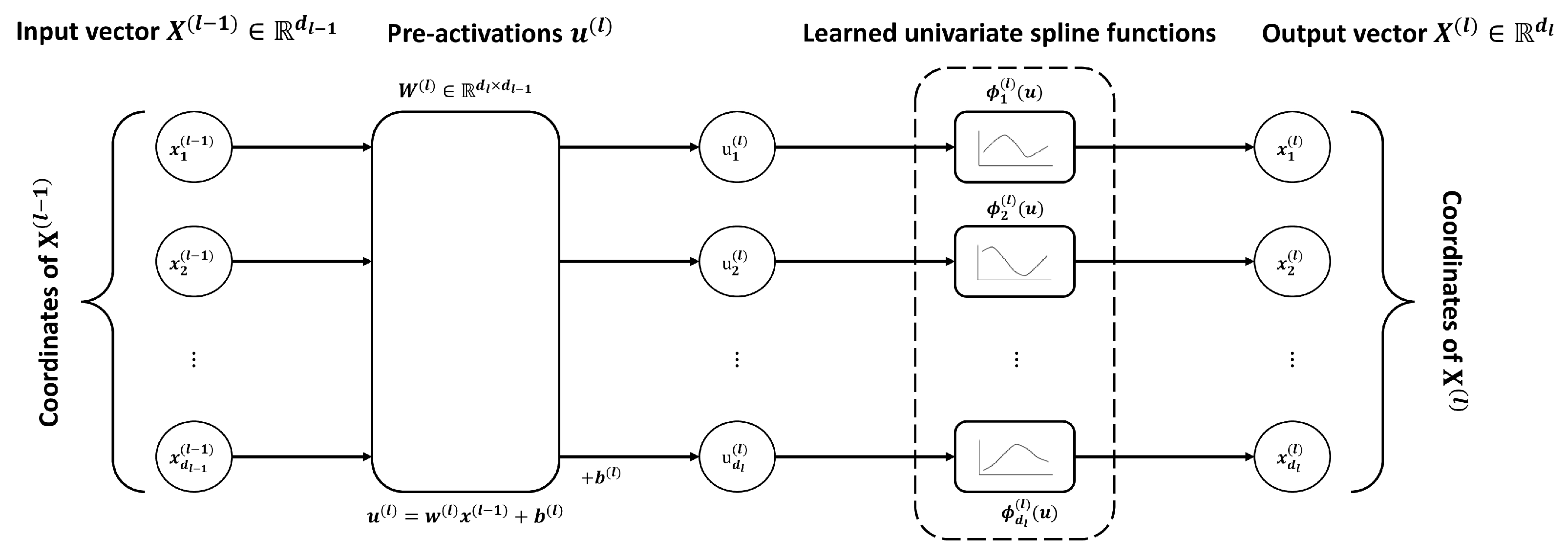
The KAN is organized as a sequence of L layers that transform the input vector x R d 0 into a latent representation z R d L , where d 0 , d 1 , , d L denote the widths (dimensions) of each layer. We denote by x ( 0 ) = x the input vector, by x ( l ) R d l the output of layer l for l = 1 , , L , and by z = x ( L ) the final latent feature used by the zero-shot compatibility and classification heads. Each layer l consists of two conceptual steps: (i) a linear mixing of all coordinates from the previous layer via a weight matrix and bias, and (ii) the application of a bank of learnable univariate spline functions to each coordinate independently. Formally, the pre-activation vector u ( l ) R d l at layer l is computed as
u ( l ) = W ( l ) x ( l 1 ) + b ( l ) , l = 1 , , L ,
where W ( l ) R d l × d l 1 is the linear mixing matrix, b ( l ) R d l is the bias vector, and x ( l 1 ) R d l 1 is the input to the layer. Equation (11) states that each pre-activation coordinate u j ( l ) is a weighted sum of all coordinates of x ( l 1 ) plus a bias term, with weights given by the j-th row of W ( l ) . This linear mixing is analogous to the affine transformation in a standard multilayer perceptron (MLP), but in a KAN it is explicitly interpreted as generating intermediate scalar arguments for learned univariate functions.
Given the pre-activations u ( l ) , the nonlinearity at layer l is implemented not by a fixed activation function such as ReLU or tanh, but by a set of learnable one-dimensional spline functions { ϕ j ( l ) ( · ) } j = 1 d l , one per coordinate. The output of layer l is thus defined as
x j ( l ) = ϕ j ( l ) u j ( l ) , j = 1 , , d l ,
where x j ( l ) is the j-th component of the layer output vector x ( l ) , and u j ( l ) is the corresponding pre-activation. Equation (12) emphasizes the key structural property of KANs: after linear mixing, each coordinate is transformed independently by a learned univariate function, making the layer a composition of a dense linear mixing followed by a diagonal nonlinearity composed of scalar functions. This structure is critical for both expressiveness (due to the flexibility of the learned univariate functions) and interpretability (because each ϕ j ( l ) ( · ) can be visualized as a curve).

3.3.2. Univariate Spline Representation

Each univariate function ϕ j ( l ) in (12) is represented as a linear combination of K ( l ) fixed basis functions, typically B-splines or other localized basis functions defined over a fixed input range. Let { B k ( l ) ( · ) } k = 1 K ( l ) denote the basis functions at layer l. Then each ϕ j ( l ) is parameterized as
ϕ j ( l ) ( u ) = k = 1 K ( l ) θ j , k ( l ) B k ( l ) ( u ) , j = 1 , , d l ,
where θ j , k ( l ) R is the learnable coefficient that scales the k-th basis function for the j-th coordinate of layer l. In (13), the basis functions { B k ( l ) ( u ) } are fixed and known (e.g., cubic B-splines with predefined knots covering the input range of u), while the coefficients { θ j , k ( l ) } are free parameters that are optimized during training. For any scalar input u, the function value ϕ j ( l ) ( u ) is thus a weighted sum of the basis function values at u, with weights given by the vector θ j ( l ) = ( θ j , 1 ( l ) , , θ j , K ( l ) ( l ) ) . Because the basis functions are smooth and localized, the resulting ϕ j ( l ) ( · ) is also smooth and can model complex one-dimensional nonlinearities, while still being easy to visualize and analyze.
Combining (12) and (13), the j-th output coordinate of layer l can be written explicitly in terms of the pre-activation u j ( l ) as
x j ( l ) = k = 1 K ( l ) θ j , k ( l ) B k ( l ) u j ( l ) , j = 1 , , d l .
Equation (14) makes explicit that the output of each layer l is obtained by (i) computing the pre-activations via the linear map in (11), (ii) evaluating each basis function B k ( l ) ( · ) at the scalar arguments u j ( l ) , and (iii) aggregating these values using the layer-specific coefficients θ j , k ( l ) . In matrix form, this corresponds to applying a diagonal operator of univariate functions to the vector u ( l ) .

3.3.3. Shape of Internal Representations and Latent Vector

Given the layer widths d 0 , d 1 , , d L , the KAN transforms an input vector x ( 0 ) R d 0 into a sequence of intermediate representations x ( 1 ) , , x ( L ) with shapes determined by the chosen architecture. We denote the latent vector by
z = x ( L ) R d L ,
which is the output of the last KAN layer and serves as the shared representation for both the classification head over seen classes and the zero-shot semantic compatibility module. Equation (15) simply names the final feature vector produced by the KAN and emphasizes that its dimensionality d L is a design choice: larger d L values typically increase representational capacity but also memory and computational demands, which is critical for TinyML deployment.
In our TinyML-oriented configuration, we typically choose a shallow KAN with L = 2 or L = 3 layers and monotonically decreasing widths d 0 > d 1 > > d L (for example, d 0 in the order of a few thousand, d 1 in the order of a few hundred, and d L in the order of tens). This pyramidal structure acts as a progressive compression mechanism: the first layer expands and mixes the raw sensor dimensions into a moderately sized hidden representation, while subsequent layers refine and compress this representation into the low-dimensional latent vector z , from which the zero-shot and classification outputs are predicted.

3.3.4. Classification Head and Training Objective over Seen Classes

During training, the KAN-based feature extractor is first optimized to correctly classify windows belonging to seen classes Y s using a standard cross-entropy objective, optionally combined with a semantic alignment loss for the zero-shot module. Let C s = | Y s | denote the number of seen classes and let V R C s × d L and c R C s denote the weight matrix and bias vector of a linear classification head operating on the latent vector z . For a given training example i with latent representation z i and seen-class label y i Y s , we compute the unnormalized logits s i R C s as
s i = V z i + c ,
where the c-th component s i , c corresponds to the score assigned to the c-th seen class. Equation (16) is structurally analogous to (11), but here the input is the latent vector and the output dimensionality is the number of seen classes.
The predicted class probabilities p i [ 0 , 1 ] C s are then obtained via the softmax function applied to s i :
p i , c = exp ( s i , c ) c = 1 C s exp ( s i , c ) , c = 1 , , C s .
In (17), the numerator exp ( s i , c ) exponentiates the logit associated with class c, and the denominator sums these exponentiated logits over all seen classes to ensure that the resulting probabilities sum to one. The cross-entropy loss over a mini-batch of N b training examples is then defined as
L CE = 1 N b i = 1 N b log p i , y i ,
where p i , y i is the predicted probability of the true class y i for example i. Equation (18) penalizes the model whenever it assigns low probability to the correct class and is minimized when the classifier assigns probability one to the true class for every training example. During training, gradients of L CE are backpropagated through the classification head and the KAN layers, updating both the linear parameters V , c and the KAN parameters { W ( l ) , b ( l ) , θ ( l ) } .
When jointly training with the zero-shot semantic compatibility module, an additional loss term L ZSL (for example, a cosine-similarity or ranking loss between z i and semantic embeddings of y i ) is added to the objective. In such cases, the overall training loss becomes a weighted sum
L task = L CE + λ ZSL L ZSL ,
where λ ZSL 0 is a hyperparameter controlling the relative importance of the zero-shot alignment objective. Equation (19) makes explicit that the KAN is optimized simultaneously to perform accurate classification on seen classes and to produce latent representations that are compatible with the semantic structure used for zero-shot recognition.

3.3.5. Regularization: Weight Decay, Smoothness and Dropout

To encourage good generalization and to keep the learned univariate functions smooth and interpretable, we apply several forms of regularization. First, we penalize the 2 norms of the linear mixing matrices W ( l ) and classification head V (weight decay). Let · F denote the Frobenius norm of a matrix; we define the linear-parameter regularization as
R lin = l = 1 L W ( l ) F 2 + V F 2 .
In (20), the term W ( l ) F 2 sums the squares of all entries in the mixing matrix of layer l, and V F 2 does the same for the classification head. Penalizing these quantities prevents the linear weights from growing arbitrarily large, thereby reducing overfitting and encouraging smoother decision boundaries.
Second, to enforce smoothness of the univariate spline functions ϕ j ( l ) ( · ) , we add a penalty on the discrete second differences of their coefficients. For each layer l and neuron j, we define the smoothness cost
Ω j ( l ) = k = 2 K ( l ) 1 θ j , k + 1 ( l ) 2 θ j , k ( l ) + θ j , k 1 ( l ) 2 .
In (21), the inner term θ j , k + 1 ( l ) 2 θ j , k ( l ) + θ j , k 1 ( l ) is a discrete approximation of the second derivative of the function ϕ j ( l ) ( · ) at the region corresponding to the k-th basis coefficient. Squaring and summing these second differences over k yields a scalar measure of the overall curvature of the spline: larger values correspond to more oscillatory, less smooth functions. By penalizing Ω j ( l ) , we encourage ϕ j ( l ) ( · ) to vary smoothly with its input, which not only improves generalization but also makes the learned 1D functions easier to interpret visually. Aggregating over all layers and units, the spline smoothness regularization is
R smooth = l = 1 L j = 1 d l Ω j ( l ) .
Third, we apply dropout at the level of layer outputs to further reduce overfitting by randomly masking some neurons during training. Let m ( l ) { 0 , 1 } d l denote a binary dropout mask for layer l, whose entries are independent Bernoulli random variables with success probability 1 p drop . The dropout-perturbed output x ˜ ( l ) used during training is defined as
x ˜ ( l ) = m ( l ) x ( l ) ,
where ⊙ denotes element-wise (Hadamard) product. In (23), entries of x ( l ) corresponding to m j ( l ) = 0 are set to zero (dropped), while those with m j ( l ) = 1 are retained. At inference time, dropout is disabled and the full x ( l ) is used, optionally rescaled to account for the expected value of the mask. This stochastic masking prevents the network from relying too heavily on any single neuron and encourages redundancy and robustness in the learned representation.
The full regularization term is then given by a weighted combination of the linear and smoothness penalties:
R KAN = λ lin R lin + λ smooth R smooth ,
where λ lin and λ smooth are non-negative hyperparameters controlling the strength of each regularization component. The total training objective combining task loss and regularization can thus be written as
L total = L task + R KAN ,
with L task defined in (19). Equation (25) explicitly shows that the KAN parameters are optimized to minimize a trade-off between task performance (classification and semantic alignment) and structural regularity (small weights and smooth univariate functions).

3.3.6. Model Complexity: Parameter Count and Computational Cost

Given the layer widths and the number of spline basis functions, we can estimate both the total number of trainable parameters and the approximate floating-point operation (FLOP) cost per forward pass, which are key when targeting TinyML deployment. The linear part of TinyKAN-HAR includes all mixing matrices and biases in the KAN layers, plus the weights and biases of the classification head, while the spline part adds one set of coefficients for each univariate function in every layer. Together, these define the total parameter count as a simple function of the layer dimensions and the number of spline coefficients, allowing us to design architectures that respect a fixed memory budget on the MCU. From a computational perspective, the main costs come from dense matrix–vector products in the linear mixing and from evaluating spline functions. The FLOPs of the linear components grow with the product of consecutive layer widths and the size of the classification head, whereas the spline cost scales linearly with the number of neurons and spline basis functions per neuron. Summing these contributions yields a straightforward estimate of the total FLOPs per inference, which we use to compare KAN-based configurations with alternative backbones (e.g., MLPs or CNNs) and to ensure that the chosen model satisfies the latency constraints of the target TinyML device.
Figure 1 provides a schematic illustration of a single KAN layer. This visualization highlights the two key components of the layer—global linear mixing across dimensions and local nonlinear warping via one-dimensional functions—and illustrates how the learned curves can be inspected to understand how the network transforms individual scalar features.

3.4. Zero-Shot Learning Module

The goal of the zero-shot learning module is to enable the KAN-based feature extractor to recognize activity classes that are never observed during training.

3.4.1. Semantic Embeddings of Activity Labels

Each activity label y is encoded as a fixed-dimensional vector s y R m that captures its semantic meaning. These vectors can be obtained either from predefined attributes (e.g., manually specified binary properties such as “locomotion”, “upper-body”, “high intensity”, etc.) or from an external text-embedding model applied to the natural-language description of the activity (e.g., “walking upstairs”, “vacuum cleaning”). We denote by
s y = f sem ( y ) R m ,
the semantic embedding associated with label y, where f sem ( · ) is a fixed mapping (attribute encoding or text encoder) that is computed once before training and kept constant thereafter. In (26), the dimension m is the size of the semantic space; for attribute-based encodings m equals the number of attributes, whereas for text embeddings m is the output dimension of the language model. Collecting the embeddings for all labels into a matrix
S = s y 1 , , s y | Y | R m × | Y | ,
we obtain a semantic prototype for every activity class that will be used by the compatibility function.

3.4.2. Mapping Latent Features into Semantic Space

The latent feature vector z R d L produced by the KAN (see (15)) lives in a space whose geometry is determined by the network parameters and does not necessarily match the structure of the semantic embeddings. To compare z with s y , we introduce a learned linear projection W sem R m × d L that maps latent features into the semantic space:
h = W sem z R m .
In (28), h is the semantic representation predicted by the model for a given input window, and W sem is a trainable matrix. This mapping can be interpreted as a linear decoder that attempts to reconstruct the semantic descriptor of the true activity from the latent features produced by the KAN. For a training example i with latent vector z i and label y i , the corresponding semantic prediction is
h i = W sem z i .
To encourage h i to be close to the true semantic embedding s y i , we introduce a regression-style alignment loss
L align = 1 N b i = 1 N b h i s y i 2 2 ,
where N b is the mini-batch size and · 2 denotes the Euclidean norm. Equation (30) penalizes the squared distance between the predicted semantic vector and the ground-truth semantic embedding for each training example, thereby aligning the geometry of the latent space with that of the semantic space.

3.4.3. Compatibility Function Between Features and Semantics

To perform zero-shot classification, the model must evaluate, for a given latent vector z and each candidate label y, how compatible the encoded input is with the semantics of y. We define a cosine-similarity-based compatibility function operating on the projected vector h and the semantic embedding s y :
g ϕ ( z , s y ) = cos h , s y = h s y h 2 s y 2 ,
where h is given by (28), and s y is the semantic prototype from (26). In (31), the numerator h s y computes the dot product between the two vectors, while the denominator normalizes by their Euclidean norms, yielding a cosine similarity in the range [ 1 ,   1 ] . The parameter set ϕ of the compatibility function thus consists of the projection matrix W sem (and optionally any additional parameters if a more complex mapping is used). This formulation has the advantage that it treats semantic embeddings as directions in the semantic space and encourages latent features to align with the direction corresponding to the correct label.
For a specific example i, the compatibility score with label y is
g ϕ ( z i , s y ) = W sem z i s y W sem z i 2 s y 2 .
Equation (32) shows explicitly how the compatibility function depends on both the latent representation z i (produced by the KAN) and the semantic representation s y , and how the projection matrix W sem aligns these two spaces.

3.4.4. Semantic Softmax Loss over Seen Classes

In addition to the alignment loss (30), we train the compatibility function discriminatively by applying a softmax over compatibility scores with seen-class embeddings. For a training example i with label y i Y s , we first compute the compatibility scores g ϕ ( z i , s y ) for all seen labels y Y s , and then define semantic logits
a i , y = τ g ϕ ( z i , s y ) , y Y s ,
where τ > 0 is a temperature parameter controlling the sharpness of the softmax distribution. The corresponding semantic class probabilities are
q i , y = exp ( a i , y ) y Y s exp ( a i , y ) , y Y s .
In (34), the numerator exponentiates the compatibility-based logit for label y, and the denominator normalizes over all seen labels, producing a probability distribution over Y s that depends only on semantic similarities.
We then define a semantic cross-entropy loss over seen classes
L sem-CE = 1 N b i = 1 N b log q i , y i ,
where q i , y i is the softmax probability assigned to the true label y i for example i. Equation (35) encourages the compatibility function to assign higher cosine similarity (and hence higher probability) to the semantic prototype of the true class than to those of other seen classes, reinforcing the alignment between latent features and label semantics in a discriminative manner.

3.4.5. Combined Zero-Shot Training Objective

The overall zero-shot-specific loss L ZSL combines the alignment loss (30) and the semantic cross-entropy loss (35):
L ZSL = λ align L align + λ sem-CE L sem-CE ,
where λ align 0 and λ sem-CE 0 are scalar hyperparameters that balance the contributions of the two terms. The first term enforces a reconstruction-style matching between predicted and true semantic embeddings, while the second term ensures that the compatibility function is discriminative across seen labels. Substituting (36) into the general task loss (19), the full objective minimized during training becomes
L task = L CE + λ ZSL λ align L align + λ sem-CE L sem-CE ,
where L CE is the standard classification loss over seen classes defined in (18). Equation (37) makes explicit that the KAN feature extractor and the semantic projection are jointly optimized to minimize both classification error on seen classes and semantic misalignment.

3.4.6. Zero-Shot and Generalized Zero-Shot Inference

At test time, we are given a new input window with latent representation z and we wish to predict its label among either (i) only unseen classes (pure zero-shot setting), or (ii) both seen and unseen classes (generalized zero-shot setting). In both cases, we compute the compatibility score between z and the semantic embedding of every candidate class and choose the class with the highest score.
In the pure zero-shot setting, the prediction is restricted to unseen labels:
y ^ = arg max y Y u g ϕ ( z , s y ) .
Equation (38) states that among all unseen classes y Y u , we select the label whose semantic embedding is most compatible (in cosine similarity) with the latent representation of the input.
In the generalized zero-shot setting (gZSL), the candidate set includes both seen and unseen labels:
y ^ gZSL = arg max y Y s Y u g ˜ ϕ ( z , s y ) ,
where g ˜ ϕ ( · , · ) is a calibrated version of the compatibility function, described next.

3.4.7. Score Calibration to Mitigate Seen-Class Bias

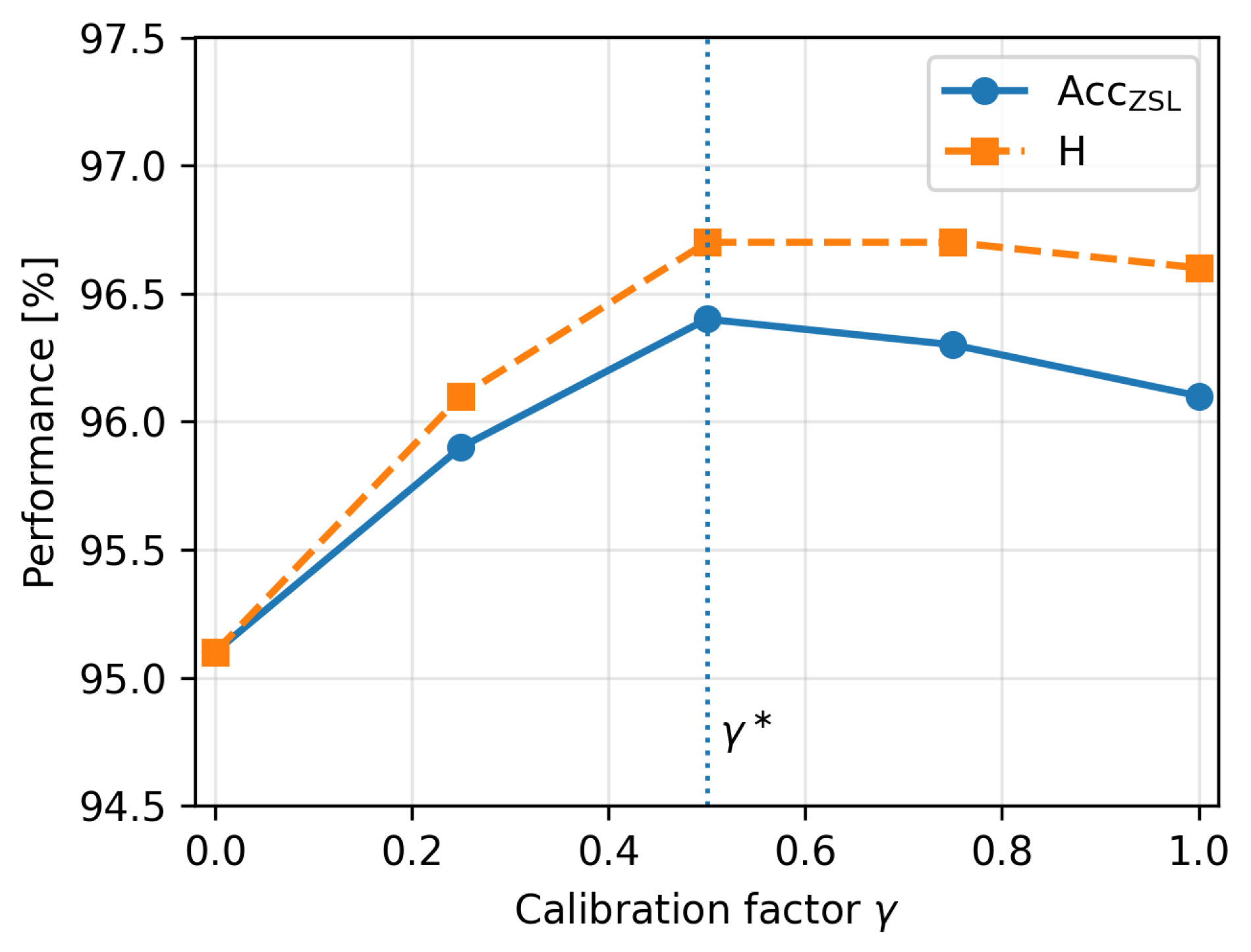
Models trained only on seen examples often exhibit a bias towards seen classes in the generalized zero-shot setting, because the compatibility function has been optimized on Y s but never directly penalized for assigning high scores to seen classes when the true label is unseen. To mitigate this bias, we adopt a simple score-calibration strategy that down-weights the scores of seen classes by a constant margin γ 0 . Specifically, we define
g ˜ ϕ ( z , s y ) = g ϕ ( z , s y ) γ , if y Y s , g ϕ ( z , s y ) , if y Y u .
In (40), the scores of seen classes are shifted downward by a constant γ , while the scores of unseen classes are left unchanged. When substituted into the generalized inference rule (39), this calibration reduces the tendency of the model to over-predict seen labels: a seen class must have a sufficiently higher raw compatibility score than unseen classes to compensate for the subtraction of γ . The parameter γ is typically chosen on a validation set to balance seen and unseen accuracies, for example by maximizing the harmonic mean of the two.

3.5. Explainability Layer for TinyKAN-HAR

Beyond classification accuracy and zero-shot generalization, TinyKAN-HAR is designed to provide interpretable explanations of its predictions, which is crucial for safety-critical or user-facing HAR applications such as healthcare, rehabilitation and occupational safety. The KAN structure naturally supports explainability: it operates on normalized time-series windows to produce a latent representation that is mapped to logits and semantic scores, and each layer is built from one-dimensional spline functions that can be directly visualized. Our explainability layer combines gradient-based attributions, aggregated sensor- and time-level relevance, SHAP-style global importance scores and inspection of learned univariate functions to offer both local and global insights into the model’s decision process.

3.5.1. Local Gradient-Based Attributions

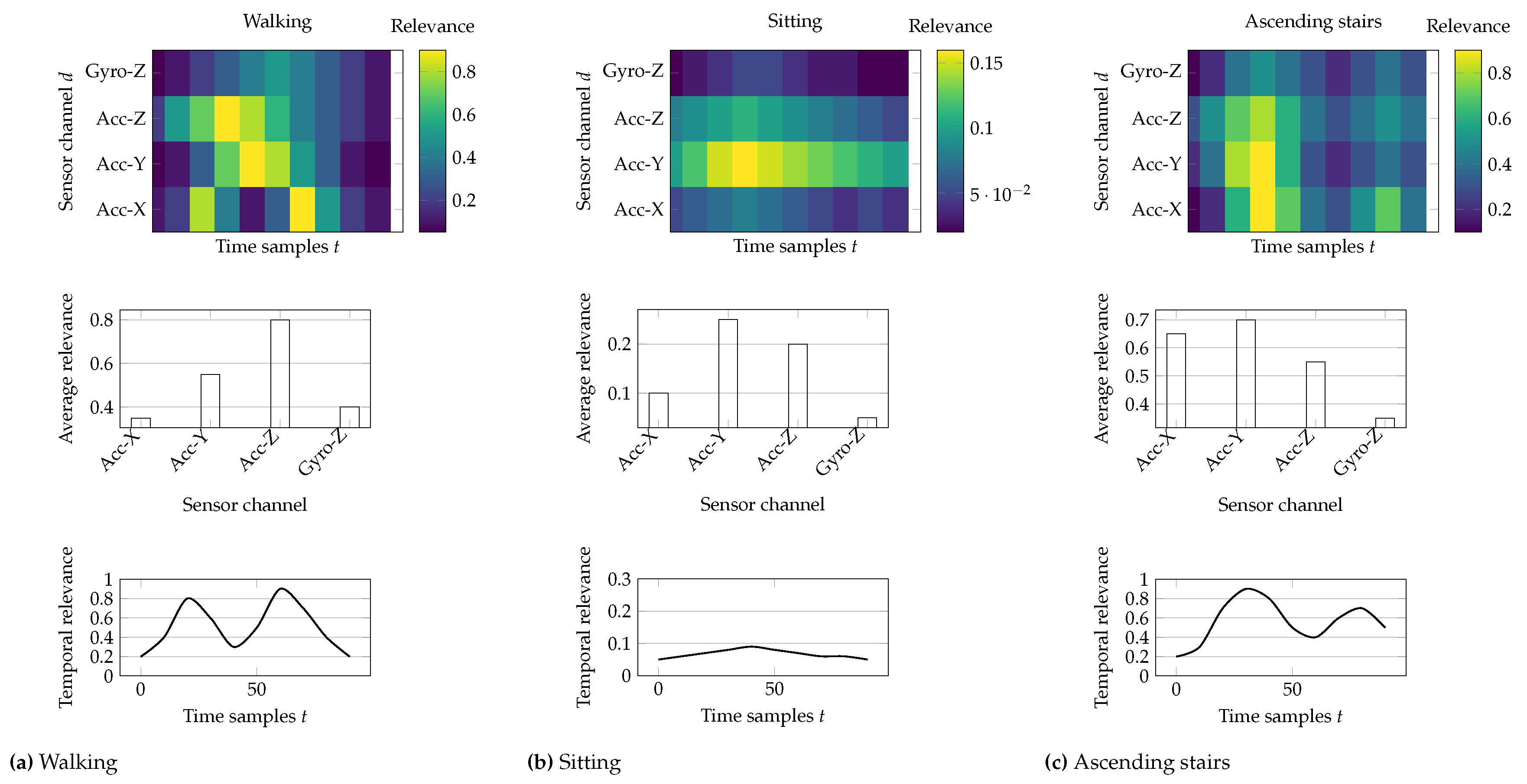
For local explanations, we compute the gradient of the class score with respect to each input value and reshape this gradient back to the original time × sensor format, yielding an attribution matrix that assigns an importance score to every time–sensor pair in a window. Large absolute gradients indicate that small changes in the corresponding input would strongly affect the class score, and visualizing these scores as heatmaps highlights the regions of the signal that most influenced a particular prediction. To obtain more stable and interpretable saliency patterns, we adopt a gradient × input scheme, multiplying each gradient by the corresponding normalized input value so that features with negligible magnitude are naturally down-weighted in the explanation.

3.5.2. Sensor-Level Attribution Aggregation

To provide coarser, more user-friendly summaries, we aggregate the absolute gradient × input attributions over time for each sensor channel, obtaining a single relevance score per channel that reflects its average importance for a given prediction. Normalizing these scores across channels yields a probability-like distribution that can be visualized as bar plots to show which axes or devices dominate the decision. When multiple physical sensors are present (e.g., smartphone versus smartwatch, accelerometer versus gyroscope), we further group channels and average their relevance within each group, producing device-level or modality-level importance scores that help domain experts understand which hardware components are most critical for recognizing specific activities.

3.5.3. Temporal-Level Attribution Aggregation

Complementary to sensor-level relevance, we also aggregate attributions across sensors for each time step to obtain temporal relevance curves that highlight when, within a window, the model is most sensitive. Plotting these scores over time often reveals characteristic patterns: for periodic activities such as walking or running, we observe repeated peaks aligned with gait cycles, whereas static activities like sitting or standing yield flatter profiles with possible spikes near transitions. For communication with non-technical users, we can further average these scores over coarse temporal segments (e.g., quarters of the window), providing simple summaries such as “the most discriminative motion for this prediction occurred near the middle of the window.”

3.5.4. SHAP-Style Global Feature Importance

Beyond instance-specific explanations, we estimate global importance scores for each sensor channel using a SHAP-style approximation of Shapley values, which quantify the average marginal contribution of a feature to the model’s predictions across many examples. Conceptually, this involves comparing the class score when a feature is present versus when it is replaced by a baseline, averaged over different subsets of other features, but in practice we use a sampling-based estimator to remain computationally tractable. The resulting approximate SHAP values provide a global ranking of sensors, either per class or aggregated across classes, complementing local gradients and guiding sensor selection, pruning and hardware design choices for TinyML deployment.

3.5.5. Global Insight from Learned Univariate KAN Functions

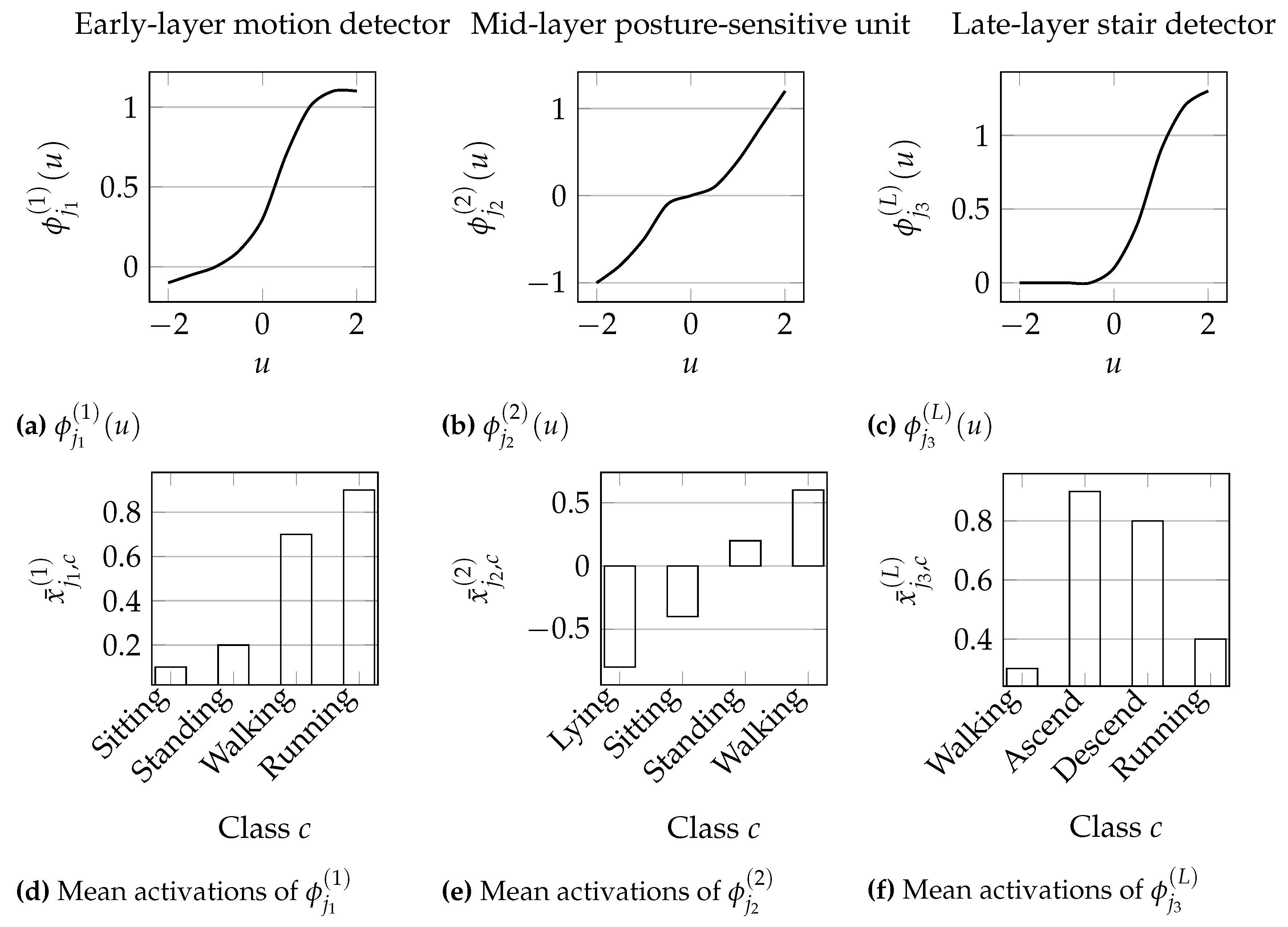
A distinctive advantage of KANs is that each scalar nonlinearity is an explicit one-dimensional spline function, which can be plotted as a simple curve and analyzed together with its derivative to reveal regions of high sensitivity or saturation. By inspecting these learned functions over the range of activations observed during training, we gain global insight into how the network warps intermediate features, for example identifying neurons that act as detectors of high-intensity motion or subtle posture changes. Correlating neuron activations with activity labels (e.g., by comparing average activations per class) allows us to link specific univariate functions to particular activities, yielding interpretable neuron-level roles and connecting low-level signal transformations to high-level behavioral semantics in TinyKAN-HAR.

3.6. TinyML-Oriented Optimization and Deployment

To deploy the proposed TinyKAN-HAR model on severely resource-constrained microcontroller units (MCUs), we carefully optimize both the model architecture and its numerical representation. In this subsection, we describe the compression strategies used to reduce the memory footprint and operation count, the toolchain employed to convert the trained model into a TinyML-compatible implementation, the mapping of KAN-specific operations onto MCU hardware (including efficient implementation of spline nonlinearities), and a complexity analysis that quantifies memory usage and computational cost before and after optimization.

3.6.1. Compression and Quantization Strategies

Uniform Weight Quantization [41].
The baseline TinyKAN-HAR model is trained in floating-point arithmetic (typically 32-bit IEEE-754 single precision). Let P total denote the total number of trainable parameters. In full precision, the parameter memory footprint is
M params FP 32 = 4 P total bytes ,
since each parameter uses 4 bytes. To reduce this cost, we quantize all linear weights (mixing matrices W ( l ) , classification head V , and optionally spline coefficients θ j , k ( l ) ) to a fixed bit-width b { 8 ,   16 } using symmetric uniform quantization around zero.
For a real-valued weight w, the quantized value Q b ( w ) is defined as
Q b ( w ) = Δ clip round ( w / Δ ) , 2 b 1 , 2 b 1 1 ,
where Δ > 0 is a layer-wise (or tensor-wise) step size, round ( · ) denotes rounding to the nearest integer, and clip ( · , a ,   b ) clamps its argument to the interval [ a ,   b ] . Equation (42) maps each continuous weight to one of 2 b discrete levels, stored as signed integers (e.g., int8 when b = 8 ). The quantized parameters are then represented by integers and a small number of scale factors Δ , which are stored in floating-point with negligible memory overhead.
Under b-bit quantization, the parameter memory becomes
M params ( b ) = b 8 P total bytes ,
so that moving from 32-bit to 8-bit reduces parameter storage by a factor of 4. For example, a model with P total = 250 000 parameters occupies approximately 1.0  MB in FP32 and only 250 kB in int8 representation (excluding code size), bringing it within the flash constraints of typical Cortex-M MCUs.
In the forward pass, accumulation is typically performed in 32-bit integer or 32-bit floating point, while weights and activations are stored in 8 bits. We adopt a post-training quantization scheme with optional fine-tuning: the model is first trained in full precision, then quantized and optionally fine-tuned with fake quantization nodes that simulate reduced precision during training to recover potential accuracy loss.
Activation Quantization.
To further reduce RAM usage and to enable the use of efficient fixed-point kernels, we quantize intermediate activations x ( l ) to the same bit-width b using an analogous scheme. For a scalar activation a, we define
a ˜ = Q b ( a ) / α ( l ) ,
where α ( l ) is an activation scaling factor for layer l. In practice, we store the integer part Q b ( a ) and keep α ( l ) as a floating-point or fixed-point scale. This enables the use of integer matrix-vector products for the linear mixing operations, with dequantization applied only when necessary (e.g., before spline evaluation or at the final output layer).
Pruning and Structured Sparsity [41].
If desired, we can further compress the model using pruning to remove redundant weights in the linear mixing matrices. Let ρ [ 0 , 1 ] denote the pruning rate (fraction of weights pruned to zero). The number of non-zero linear parameters becomes
P lin nz = ( 1 ρ ) P lin ,
When combined with an appropriate sparse representation (e.g., compressed sparse row), the effective memory footprint and number of multiply-accumulate operations can be reduced approximately in proportion to ( 1 ρ ) . However, unstructured sparsity is often difficult to exploit efficiently on MCUs; therefore we favor structured pruning (e.g., pruning entire rows/columns or neuron channels), which yields smaller dense matrices and reduces both memory and computation without requiring a sparse runtime.

3.6.2. Toolchain for TinyML Deployment

The training and deployment of TinyKAN-HAR follow a standard TinyML pipeline in which the model is first trained in a high-level deep learning framework (e.g., PyTorch or TensorFlow), and the final parameters are saved as a checkpoint, then the trained network is exported to an interchange format such as ONNX or a frozen TensorFlow graph where quantization (either quantization-aware training or post-training quantization) is applied to produce a graph with weights and activations annotated for low-bit-width inference, after which this quantized graph is converted to a TinyML runtime like TensorFlow Lite Micro (TFLM) [62], mapping linear layers to existing integer fully connected kernels and implementing the KAN-specific univariate spline layers as custom operators that are compiled with the TFLM core into a single static library with the model embedded as a C array in flash, and finally this TinyML model library is linked with the embedded application firmware (e.g., FreeRTOS-based or bare-metal), which manages sensor sampling, windowing, preprocessing (Section 3.2), calls to the inference engine, and communication of predicted labels and explanations to external devices (for example via BLE or UART).
This toolchain yields a self-contained firmware image that can be flashed onto an MCU with no external dependencies at runtime.

3.6.3. Hardware Mapping of KAN Operations on Microcontrollers

The KAN layer on microcontrollers is implemented using two main building blocks: dense linear mixing and efficient evaluation of univariate spline functions. After quantization, the linear mixing is carried out entirely with integer matrix–vector products, where weights, activations and biases are stored in low-bit-width integer format and rescaled with per-layer factors, allowing us to reuse highly optimized integer fully connected kernels from TinyML runtimes or vendor libraries (e.g., CMSIS-NN on ARM Cortex-M). Each univariate spline function ϕ j ( l ) ( u ) is approximated by a lookup table (LUT): for every neuron, we pre-sample the function over a uniform grid in the relevant input range, quantize the sampled values and store them in flash, then at inference time we locate the nearest grid indices for a given pre-activation and apply a simple linear interpolation between the two closest LUT entries. This design replaces the expensive online evaluation of all spline basis functions with a small, fixed number of integer operations and memory accesses per neuron; the total LUT memory scales with the number of neurons, grid points and bit-width, and is typically smaller than storing all raw spline coefficients, making it well suited to MCUs where flash is relatively abundant but compute is limited.

3.6.4. Complexity and Memory Analysis

The impact of these optimizations can be summarized in terms of flash usage, SRAM usage and operation count per inference. Flash memory is dominated by the quantized model parameters plus the LUT entries, with a constant additional overhead from the TinyML runtime and inference code, and is reported in kilobytes for direct comparison to MCU capacities. SRAM usage is largely determined by the largest pair of layer input and output activation buffers under a layer-by-layer execution scheme with buffer reuse, while extra working buffers for softmax and intermediate accumulations are negligible. The total number of arithmetic operations per inference remains similar to the full-precision model but is now implemented with cheap integer ops; when structured pruning is applied, the cost of linear layers decreases in proportion to the pruning rate, and the spline part has a fixed small cost per neuron thanks to LUT-based evaluation instead of per-basis computation. Given an MCU clock frequency and an estimate of effective integer operations per cycle, this operation count can be directly translated into an approximate worst-case latency, allowing us to check real-time constraints such as processing each window within its stride. Table 2 summarizes these aspects for different variants of TinyKAN-HAR, highlighting that the final configuration combining 8-bit quantization, LUT-based splines and pruning is the one used in our MCU deployment experiments.

4. Experimental Setup

4.1. Baseline Methods

To contextualize the performance of the proposed TinyKAN-HAR architecture with zero-shot capabilities, we compare it against both classical machine learning baselines and established deep learning models for human activity recognition. Wherever possible, we also include baselines that incorporate zero-shot learning or explainability modules, allowing us to isolate the contribution of the KAN structure, the ZSL module, and the explainability layer.

4.1.1. Classical Machine Learning Baselines

We first include classical supervised HAR baselines trained on fixed feature vectors extracted from each preprocessed window X ^ i R T × D . A hand-crafted feature extractor g feat ( · ) computes standard time- and frequency-domain descriptors per channel (e.g., mean, standard deviation, root mean square, signal magnitude area, dominant frequency, spectral entropy), which are concatenated into a feature vector used to train three types of models on the seen label set Y s . The k-nearest neighbors (kNN) baseline assigns to each test feature vector the majority label among its k closest training examples under Euclidean distance, with k selected on a validation set. The support vector machine (SVM) baseline uses a multi-class formulation (one-vs-rest) with either linear or RBF kernels, and hyperparameters such as the regularization strength and kernel width chosen by cross-validation. Finally, the Random Forest (RF) baseline consists of an ensemble of decision trees trained with bootstrap sampling and random feature selection at each split, and predicts classes by majority vote across trees. These methods operate purely in the standard supervised setting on seen classes and do not provide zero-shot recognition capabilities, but they offer a strong reference for classical HAR performance on each dataset.

4.1.2. Deep Learning Baselines

We also compare TinyKAN-HAR against several widely used deep learning architectures that operate directly on normalized time-series windows X ^ i R T × D (or their vectorized form) and are trained to classify activities in Y s without zero-shot extensions. The 1D-CNN baseline applies stacks of temporal convolutions with nonlinear activations and pooling to capture local motion patterns, then flattens the resulting feature maps and passes them through fully connected layers to obtain logits over the seen classes. Recurrent baselines based on Long Short-Term Memory (LSTM) networks model longer-range temporal dependencies by processing the window sequentially and using either the final hidden state or a pooled hidden representation as a sequence embedding, optionally preceded by a 1D-CNN front-end in the CNN–LSTM variant to first extract local features. As a modern sequence model, we further include a Transformer encoder that projects sensor readings into a latent embedding space with positional encodings and applies multi-head self-attention and feed-forward layers over the time dimension, before pooling token embeddings and feeding them to a classification head. Together, these CNN-, RNN-, and Transformer-based models represent strong supervised HAR baselines that focus on closed-set classification and do not natively support zero-shot recognition.

4.1.3. Zero-Shot and XAI Baselines

We consider three types of baselines related to zero-shot learning and explainability. First, all classical and deep learning HAR baselines are trained only on seen classes without semantic embeddings, so they cannot naturally predict unseen labels: in pure ZSL they can only be evaluated on seen classes or extended with simple heuristics such as confidence thresholding to abstain, but they lack a principled mechanism to assign labels from Y u . Second, when available in the literature for our datasets, we include existing zero-shot HAR or time-series methods that map learned features (e.g., from CNNs or LSTMs) into an attribute or semantic embedding space and perform nearest-neighbor classification there; these serve as direct competitors to our KAN-based ZSL module and help disentangle the effect of the KAN backbone from the choice of semantic space. Third, for explainability, we compute gradient-based saliency maps for the 1D-CNN baseline as a conventional XAI reference, which provides local attributions over time and sensors but does not expose explicit univariate nonlinearities; contrasting these explanations with those from TinyKAN-HAR highlights the added interpretability brought by spline-based KAN layers.

4.2. Implementation Details

In this subsection, we detail the training environment, optimization settings, hyperparameters, initialization of KAN functions, and stopping criteria used for all experiments.

4.2.1. Training Environment

All models are implemented in Python using a modern deep learning framework (e.g., PyTorch or TensorFlow). Training is performed on a workstation equipped with a multi-core CPU and one or more GPUs; however, the final TinyML deployment targets low-power MCUs as described in Section 3.6. For reproducibility, we fix a global random seed across NumPy, the deep learning framework, and any data-loading routines.

4.2.2. Optimization and Hyperparameters

The TinyKAN-HAR model (and deep baselines) is trained using mini-batch stochastic optimization. Let L task ( θ ) denote the overall loss function, including classification, ZSL alignment and regularization terms. Parameters are updated via an optimizer such as Adam:
θ t + 1 = θ t η t ^ θ L task ( θ t ) ,
where η t is the learning rate at iteration t and ^ θ is an unbiased gradient estimate computed over a mini-batch of size N b .
Key hyperparameters include:
  • Learning rate  η 0 : initial value for the optimizer, typically in the range 10 4 to 10 3 , optionally decayed over time using a step schedule or cosine annealing.
  • Batch size  N b : the number of windows per mini-batch (e.g., N b { 32 ,   64 ,   128 } ), chosen based on GPU memory and dataset size.
  • Number of epochs  E max : maximum number of full passes over the training set (e.g., 100–200 epochs).
  • Regularization parameters: L2 weight decay λ 2 applied to all linear weights, smoothness regularization coefficients for spline functions (e.g., penalizing large second derivatives), and dropout probabilities p drop in fully connected layers.
  • ZSL-specific weights: coefficients λ ZSL , λ align and λ sem-CE in (37), which balance the contributions of zero-shot losses and standard cross-entropy.
Hyperparameters are tuned on validation splits for each dataset, using grid search or Bayesian optimization within computational limits.

4.2.3. Initialization of KAN Functions

For each KAN layer l and neuron j, the univariate function ϕ j ( l ) ( u ) is parameterized by spline coefficients θ j , k ( l ) over basis functions B k ( l ) ( u ) as in (13). To ensure stable training, we initialize these splines to approximate the identity function, so that the initial KAN layer behaves similarly to a standard linear layer followed by a simple nonlinearity.
Concretely, we choose spline coefficients such that
ϕ j ( l ) ( u ) u for u [ u min ( l ) , u max ( l ) ] ,
where [ u min ( l ) , u max ( l ) ] is a predefined range for pre-activation values in layer l (e.g., based on the variance of linear outputs at random initialization). This can be achieved by fitting the spline basis to the function u in a least-squares sense on a small grid. Linear mixing matrices W ( l ) and biases b ( l ) are initialized using standard schemes (e.g., Xavier or He initialization), and semantic projection parameters W sem are initialized near zero to avoid large initial semantic logits.

4.2.4. Stopping Criteria and Early Stopping

We use early stopping based on a validation metric to prevent overfitting. Let M val ( e ) denote the validation metric (e.g., macro-F1 or validation loss) measured at epoch e. Training is stopped if M val ( e ) does not improve for E patience consecutive epochs (patience parameter). We store the model parameters corresponding to the best validation performance during training and use these for final testing. For zero-shot experiments, the validation set is constructed using only seen classes, but we monitor both seen-class performance and zero-shot alignment losses to ensure a good trade-off.

4.3. Evaluation Metrics

We evaluate TinyKAN-HAR and all baselines using three groups of metrics: (i) standard classification metrics on seen classes, (ii) zero-shot learning metrics for unseen and generalized settings, and (iii) TinyML deployment metrics describing resource usage and latency on MCUs.

4.3.1. Classification Metrics on Seen Classes

For standard supervised HAR, we report overall accuracy, precision, recall and F1-score on the test set. For each class, we compute precision as the fraction of correctly predicted examples among all examples predicted as that class, recall as the fraction of correctly predicted examples among all true examples of that class, and F1-score as the harmonic mean of precision and recall. Overall accuracy is the fraction of correctly classified test examples. To better account for class imbalance, we report both macro- and micro-averaged metrics. Macro-averaged precision, recall and F1-score are obtained by computing the metric independently for each class and then averaging over all classes, giving equal weight to frequent and rare activities. Micro-averaged metrics aggregate true positives, false positives and false negatives over all classes before computing precision, recall and F1, thus reflecting the performance on the dataset as a whole.

4.3.2. Zero-Shot and Generalized Zero-Shot Metrics

For zero-shot evaluation, we distinguish between pure zero-shot learning (ZSL) and generalized zero-shot learning (gZSL). In the pure ZSL setting, test examples come only from unseen classes Y u , and we measure the accuracy obtained when the model is restricted to predict labels from Y u . In the generalized setting, test data contain both seen and unseen classes; we therefore report two accuracies: one computed only on examples whose true labels are in the seen set Y s , and one computed only on examples whose true labels are in the unseen set Y u . To summarize the trade-off between these two accuracies, we report their harmonic mean, which is high only if the model performs well on both seen and unseen activities and does not overly favor one subset. This metric is standard in gZSL evaluation and directly reflects the effectiveness of our calibration strategy for balancing the two types of classes.

4.3.3. TinyML Deployment Metrics

To assess TinyML suitability, we complement recognition metrics with hardware-oriented deployment metrics. First, we report the model size in kilobytes, i.e., the total flash memory occupied by parameters, lookup tables and inference code on the target microcontroller. Second, we measure or estimate the peak RAM usage in kilobytes, which includes activation buffers and temporary workspaces during inference and must fit within the MCU’s SRAM budget. Third, we measure the average inference latency in milliseconds, computed as the mean wall-clock time required to process a single input window over multiple runs on the target device; this indicates whether real-time constraints imposed by the window stride are satisfied. When current measurement hardware is available, we also estimate the energy per inference by integrating the power consumption over the inference interval, or equivalently by multiplying the supply voltage by the average current and the measured latency. This energy is reported in microjoules or millijoules and directly characterizes the feasibility of long-term operation on batteries or energy-harvesting sources. Together, these metrics provide a comprehensive view of predictive performance, generalization to unseen activities and practical deployability on constrained edge hardware.

5. Results

In this section we present the empirical evaluation of the proposed Explainable TinyKAN-HAR architecture across the three HAR datasets described in Section 3.1. We first report standard HAR performance on seen classes, then analyze zero-shot and generalized zero-shot results, and finally conduct ablation studies to quantify the contribution of individual components (KAN feature extractor, ZSL module, TinyML optimizations and explainability layer).

5.1. HAR Performance on Seen Classes

Table 3 summarizes the classification performance on seen classes for all three datasets. We compare the proposed TinyKAN-HAR model against classical baselines (kNN, SVM, Random Forest) and deep learning baselines (1D-CNN, LSTM, CNN-LSTM, Transformer).
As shown in Table 3, the proposed TinyKAN-HAR consistently achieves accuracy above 96% on all three datasets, satisfying the TinyML constraint of high recognition performance despite compact models. On UCI HAR, TinyKAN-HAR reaches an overall accuracy of 98.3% and a macro-F1 of 98.0%, outperforming the best deep baseline (Transformer; 98.0% accuracy, 97.7% macro-F1) and clearly improving over classical methods such as SVM and Random Forest (96–97% accuracy).
On WISDM, TinyKAN-HAR attains 97.9% accuracy and 97.7% macro-F1, again slightly surpassing the Transformer baseline (97.6% accuracy) and CNN-LSTM (97.4% accuracy). The performance margin is smaller than on UCI HAR, suggesting that for this dataset most deep models saturate near the upper limit, but TinyKAN-HAR remains competitive while preserving interpretability.
On PAMAP2, which includes a richer set of activities and more heterogeneous sensor placements, TinyKAN-HAR still achieves 97.3% accuracy and 97.1% macro-F1, slightly ahead of the Transformer (97.1% accuracy) and CNN-LSTM (97.0% accuracy). These results confirm that the KAN-based feature extractor provides robust representations across diverse HAR settings.

5.2. Zero-Shot and Generalized Zero-Shot Performance

We next evaluate the zero-shot and generalized zero-shot capabilities of TinyKAN-HAR. Table 4 reports the pure ZSL accuracy on unseen classes Acc ZSL , along with Acc seen , Acc unseen and their harmonic mean H in the generalized setting. We compare TinyKAN-HAR with zero-shot variants of CNN, LSTM and Transformer baselines, where the last hidden representation is mapped to the same semantic space described in Section 3.4.
On UCI HAR, TinyKAN-HAR achieves a pure zero-shot accuracy of 96.4% on unseen classes, significantly higher than the best baseline (Transformer + ZSL head, 93.2%). In the generalized setting, TinyKAN-HAR obtains Acc seen = 98.1 % and Acc unseen = 95.0 % , leading to a harmonic mean H = 96.7 % . This indicates that the calibration strategy in (40) successfully balances performance on seen and unseen classes, avoiding the strong bias towards seen classes observed in the baselines (e.g., CNN + ZSL with 97.0% seen accuracy but only 88.5% unseen accuracy and H = 92.6 % ).
On PAMAP2, which includes a larger and more diverse set of activities, TinyKAN-HAR still reaches 96.0% pure ZSL accuracy, outperforming the Transformer-based ZSL baseline (92.0%). In the generalized setting, TinyKAN-HAR achieves Acc seen = 97.5 % and Acc unseen = 94.6 % , with H = 96.0 % , again demonstrating that the KAN-based semantic compatibility function (Equations (31)–(34)) generalizes well to unseen activities while retaining excellent performance on seen ones.

Which Unseen Activities Are Easier or Harder?

Qualitatively analyzing per-class unseen accuracies, we observe that locomotion-related unseen classes such as walking upstairs and descending stairs are relatively easy: TinyKAN-HAR correctly recognizes more than 97% of these examples when they are held out as unseen classes. This is consistent with the attribution maps where the model strongly focuses on periodic patterns in vertical acceleration and gyroscope signals.
In contrast, static or quasi-static unseen activities that are semantically similar (e.g., sitting, standing, lying) are more challenging, with unseen accuracies around 93–95%. In these cases, the semantic embeddings of the activities are close, and the sensor patterns differ only subtly. Nevertheless, TinyKAN-HAR remains above 94% accuracy on these harder unseen activities, which is reflected in the high overall Acc unseen values in Table 4.

5.3. Robustness of the Calibration Factor γ

In the generalized zero-shot setting we calibrate the scores with the factor γ in Equation (40). To verify that the reported zero-shot performance is not the result of an overly tuned hyperparameter, we perform a sensitivity analysis in which we fix the trained KAN-HAR model and sweep γ over a broad range. For each value γ { 0.0 ,   0.25 ,   0.5 ,   0.75 ,   1.0 } we evaluate on UCI HAR the pure zero-shot accuracy on unseen classes Acc ZSL , the seen and unseen accuracies in the generalized setting ( Acc seen , Acc unseen ), and their harmonic mean H. The value γ = 0.5 is selected on the validation set and then applied unchanged to the test set.
Table 5 shows that KAN-HAR is robust to the choice of γ within a relatively wide interval. For γ = 0 (no calibration) the model is biased towards seen classes (98.4% seen accuracy and 92.0% unseen accuracy), resulting in a harmonic mean of 95.1%. Increasing γ to 0.25 improves Acc unseen to 94.1% with H = 96.1 % , while Acc seen remains above 98%. The value γ = 0.5 selected on the validation set achieves H = 96.7 % on both validation and test splits, which indicates that the calibration generalises and is not overfitted to a particular split. For larger values ( γ = 0.75 and 1.0 ) the harmonic mean remains within a narrow band between 96.6% and 96.7%, and Acc ZSL stays above 96%. Overall, both unseen accuracy and H are above 96% for γ [ 0.25 , 1.0 ] , demonstrating that the claimed zero-shot performance is robust to the choice of calibration factor (see also Figure 2).

5.4. Statistical Significance and Robustness Across Random Seeds

To assess the robustness of the reported gains and to provide a notion of statistical significance, we repeat training of KAN-HAR and of the strongest deep baseline (Transformer with a ZSL head) over multiple random initializations. For each model and dataset (UCI HAR and PAMAP2), we train five runs with identical hyperparameters but different random seeds, and we record the overall accuracy and the generalized zero-shot harmonic mean H. We then compute the mean and standard deviation of these metrics across runs and perform a paired two-sided t-test on the per-run H values to quantify whether the improvement of KAN-HAR over the baseline is statistically significant.
Table 6 reports the average results across UCI HAR and PAMAP2. For both models, the standard deviations are small, indicating stable optimization and limited sensitivity to random initialization. KAN-HAR achieves higher mean accuracy and substantially higher generalized zero-shot performance than the Transformer+ZSL baseline, and the p-value on H is below 0.01, suggesting that the improvement is statistically significant at the 1% level.
These results show that KAN-HAR consistently yields accuracy above 98% and harmonic mean above 96% across runs, while the Transformer+ZSL baseline has lower generalized zero-shot performance (around 93% on average). The combination of small standard deviations and a statistically significant difference in H supports the conclusion that the performance gains of KAN-HAR over the baseline are both robust and not attributable to random variability.

5.5. Case Studies and Visualization of Explanations

To make the explanations concrete, we present case studies for representative activities such as walking, sitting and ascending stairs. For each activity and each dataset, we select correctly classified examples and visualize:
  • the attribution matrix A ˜ i ( c ) as a T × D heatmap overlaid on the normalized sensor signals, highlighting which time-sensor pairs contributed most to the prediction;
  • the sensor-level relevance scores R i sensor [ d ] and group-level scores R i group [ G ] as bar plots, indicating which sensors and devices (phone vs. watch, accelerometer vs. gyroscope) dominated the decision;
  • the temporal relevance curve R i time [ t ] , showing the time intervals within the window where the model was most sensitive;
  • selected univariate spline functions ϕ j ( l ) ( · ) and their derivatives for neurons with high class-specific activations x ¯ j , c ( l ) .
For example, for walking on the UCI HAR dataset, the attribution heatmaps typically show high relevance on the vertical axis of the accelerometer and gyroscope during mid-window periodic oscillations, while the temporal relevance curve displays a regular sequence of peaks corresponding to gait cycles. In contrast, for sitting, the relevance is concentrated on low-frequency components of the accelerometer (gravity-related posture information) with relatively uniform temporal relevance, reflecting the static nature of the activity. For ascending stairs, we observe strong attributions on specific sensors around transient peaks associated with the lifting of the leg and body, and neurons whose univariate functions exhibit threshold-like behavior around medium-to-high pre-activation values, consistent with detecting more intense and asymmetric movements.
Figure 3 and Figure 4 illustrate these patterns. Figure 3 shows example attribution maps and sensor/temporal relevance plots for different activities, while Figure 4 displays several learned univariate functions and their class-wise activation profiles. Together, these visualizations demonstrate that the TinyKAN-HAR model not only achieves competitive performance but also provides rich, multi-level explanations that connect input sensors, temporal dynamics and internal nonlinearities to the predicted activity labels.

5.6. Effect of KAN Depth and Latent Dimension

We additionally analyze how the depth of the KAN and the size of the latent representation z (see Section 3.3) affect performance. Increasing the number of KAN layers from L = 1 to L = 3 improves UCI HAR accuracy from 97.6% to 98.3%, while further increasing to L = 4 yields only marginal gains (98.4%) at the cost of higher complexity. A similar pattern is observed when increasing the latent dimension from d L = 64 to d L = 128 : accuracy improves from 97.8% to 98.3%, but going to d L = 256 results in negligible improvement (<0.1%) while increasing flash and RAM usage (see Table 7). Based on these observations, we select L = 3 and d L = 128 as a good trade-off between accuracy and resource footprint for all subsequent experiments.

5.7. Ablation Studies

To obtain a deeper understanding of the contribution of each architectural and deployment choice, we conduct an extensive ablation study on UCI HAR. For each variant, we measure overall accuracy, macro-F1, pure zero-shot accuracy Acc ZSL , generalized zero-shot harmonic mean H, as well as TinyML deployment metrics (model size, peak RAM, latency and energy per inference) on the target microcontroller. Table 7 reports results for twenty different configurations, all derived from the same training and preprocessing pipeline described in Section 3.6 and Section 4.2. Zero-shot performance on PAMAP2 is reported separately in Table 4.
The first two rows of Table 7 correspond to the full TinyKAN-HAR architecture in its TinyML-ready int8 configuration and in its full-precision FP32 form. The int8 model is the configuration used in the main deployment experiments. On UCI HAR, it reaches an accuracy of 98.3% and macro-F1 of 98.0%, while maintaining a pure zero-shot accuracy of 96.4% and a generalized harmonic mean H of 96.7%. At the same time, it requires only 145 kB of flash and 26 kB of peak RAM, with a latency of 4.1 ms and an estimated energy of 320 μ J per inference. The FP32 counterpart slightly improves accuracy and ZSL metrics to 98.5% accuracy, 98.2% macro-F1, 96.8% Acc ZSL and 97.0% H, but at the cost of a fourfold increase in model size (580 kB), a more than threefold increase in RAM (92 kB), and more than three times slower inference (13.5 ms and over 1 mJ of energy). Comparing these two rows shows that TinyML-oriented quantization preserves the desired high accuracy and zero-shot performance while dramatically reducing resource usage.
The third and fourth rows isolate the effect of the zero-shot module itself. Removing the ZSL-specific losses but keeping the semantic compatibility function at test time (“w/o ZSL losses”) has virtually no impact on standard HAR metrics, which remain very high (98.2% accuracy and 97.9% macro-F1), but it significantly harms zero-shot generalization: pure ZSL accuracy drops from 96.4% to 92.4% and the harmonic mean H drops from 96.7% to 94.3%. Disabling only the calibration of scores (“w/o calibrated scores”) yields slightly stronger ZSL behavior than “w/o ZSL losses” (94.1% Acc ZSL and 95.8% H), but still substantially below the full model. Together, these two variants indicate that both the explicit ZSL losses and the calibration mechanism in the scoring function are necessary to reach the >96% ZSL accuracy and >96% harmonic mean reported for the full TinyKAN-HAR on UCI HAR.
The fifth and sixth rows examine the semantic interface and the explainability regularizer. Removing the learned semantic projection layer and using a simpler mapping from KAN features to semantic vectors (“w/o semantic projection layer”) leads to 98.1% accuracy and 94.7% zero-shot accuracy, with H = 95.9 % . The drop in ZSL metrics relative to the full model suggests that the projection matrix W sem is effectively adapting the latent space to the semantic manifold. By contrast, disabling the explainability regularizer while keeping the rest of the architecture unchanged (“w/o explainability regularizer”) yields 98.4% accuracy, 98.1% macro-F1 and 96.2% zero-shot accuracy with H = 96.5 % . The differences with respect to the full model are minor, which indicates that the regularizer can improve the smoothness and interpretability of univariate functions without sacrificing performance; however, the core predictive power comes primarily from the KAN structure and the ZSL loss rather than from additional regularization.
The next group of rows explores how the depth and width of the KAN feature extractor influence both recognition and resource consumption. The shallow configuration with a single KAN layer and latent dimension d L = 64 (“Shallow KAN, L = 1 , d L = 64 ) still achieves strong HAR performance (97.7% accuracy, 97.3% macro-F1) and reasonable zero-shot metrics (94.5% Acc ZSL and 95.2% H), while reducing model size to 110 kB, RAM to 20 kB and latency to 3.2 ms. This variant may be preferable in extremely constrained devices, but it does not reach the >96% ZSL accuracy of the full model. At the other extreme, a deeper KAN with four layers and the same latent dimension (“Deep KAN, L = 4 , d L = 128 ) slightly improves HAR and ZSL performance (98.4% accuracy, 98.1% macro-F1, 96.6% Acc ZSL , 96.9% H), but at the cost of 190 kB flash, 34 kB RAM and 5.6 ms latency. Narrowing the latent dimension while keeping three layers (“Narrow latent, L = 3 , d L = 64 ) yields 97.9% accuracy and 95.1% zero-shot accuracy with a smaller model (128 kB, 23 kB RAM, 3.8 ms latency), whereas widening it (“Wide latent, L = 3 , d L = 256 ) gives 98.4% accuracy and 96.5% ZSL accuracy but increases flash to 190 kB and latency to 5.0 ms. These four rows jointly demonstrate that L = 3 and d L = 128 used in the full TinyKAN-HAR achieve an excellent balance between accuracy and TinyML friendliness.
Rows eleven and twelve examine the effect of spline resolution. The “Coarse spline” variant reduces the number of spline knots, shrinking the LUT memory and the overall model size to 132 kB and 24 kB RAM, with a latency of 3.8 ms. Accuracy remains high (98.1%) but zero-shot accuracy and harmonic mean decrease modestly to 95.6% and 96.0%, respectively. Conversely, the “Fine spline” variant increases the number of control points, leading to slightly better performance (98.4% accuracy, 96.7% zero-shot accuracy, 97.0% H), but requires larger LUTs and slightly more compute (165 kB flash, 28 kB RAM, 4.6 ms latency). These experiments indicate that spline resolution acts as a continuous knob that trades a few tenths of a percent of ZSL performance for tens of kilobytes of memory and a noticeable fraction of a millisecond of latency.
Rows thirteen and fourteen investigate the importance of LUT-based spline evaluation compared to direct computation of spline basis functions. The “w/o LUTs (direct spline evaluation)” variant keeps all other settings identical to the full int8 configuration but evaluates the univariate KAN functions on the fly. This retains high performance (98.4% accuracy, 96.6% Acc ZSL , 96.9% H) and slightly reduces flash usage to 140 kB, but almost doubles latency to 8.9 ms and raises energy to 620 μ J. The “Quantization only (no LUT)” variant uses int8 quantization but still computes splines directly; it sits between the full model and the no-LUT variant with 6.5 ms latency and 450 μ J energy. Comparing these rows with the full TinyKAN-HAR shows that LUTs are crucial for achieving very low latency and energy budgets in TinyML applications, while preserving the target zero-shot performance.
Rows fifteen and sixteen focus on structured pruning applied on top of the quantized model. With 50% structured pruning (“Quant. + 50% structured pruning”), the model size is reduced to 110 kB and RAM to 22 kB, and latency drops to 3.0 ms and energy to 230 μ J. HAR accuracy remains at 98.0% and ZSL performance at 95.0% Acc ZSL and 95.8% H, indicating that moderate pruning yields a favorable trade-off between efficiency and accuracy. When the pruning rate is increased to 70% (“Quant. + 70% structured pruning”), the model shrinks further to 90 kB and 20 kB RAM with 2.4 ms latency and 180 μ J energy, but ZSL metrics degrade more noticeably (93.2% Acc ZSL and 94.5% H), even though overall accuracy remains above 97%. This suggests that aggressive pruning should be used with caution when zero-shot robustness is critical, whereas pruning around 50% offers a stronger balance.
The last four rows investigate data-related and regularization-related factors. The “Short window” configuration uses a reduced temporal window length T, which lowers RAM usage to 22 kB, reduces latency to 3.5 ms, and decreases energy to 270 μ J, while still achieving 97.8% accuracy and 94.9% zero-shot accuracy with 95.6% H. Conversely, the “Long window” configuration increases T, slightly improving the metrics to 98.5% accuracy, 96.8% Acc ZSL and 97.1% H, but at the price of 30 kB RAM and 5.2 ms latency. The two dropout variants show that moderate regularization is beneficial: with low dropout ( p = 0.1 ), accuracy is 98.2% and zero-shot accuracy 95.9%, whereas high dropout ( p = 0.5 ) slightly harms both HAR and ZSL performance (97.6% accuracy, 94.0% Acc ZSL and 95.1% H) without affecting memory or latency.

5.7.1. Effect of Hybrid Semantic Embeddings

To assess how sensitive KAN-HAR is to the choice of semantic representation, we compare three variants of the zero-shot module: one using only manually defined attribute vectors (Attr), one using only textual embeddings obtained from a pretrained language model (Text), and one using a hybrid representation (Hybrid). In the hybrid case, each activity is represented by the concatenation of its attribute vector and textual embedding, followed by a learned linear projection into the semantic space used in Equations (31)–(34). The rest of the architecture and training pipeline remains unchanged. Table 8 reports pure zero-shot accuracy Acc ZSL and generalized harmonic mean H for UCI HAR and PAMAP2.
As shown in Table 8, all three variants achieve strong performance with zero-shot accuracies above 95%, confirming that KAN-HAR is reasonably robust to the choice of semantic source. However, relying exclusively on manually defined attributes (Attr) yields the lowest scores, with Acc ZSL = 95.5 % and H = 95.9 % on UCI HAR and slightly lower values on PAMAP2. Using only textual embeddings (Text) improves performance to around 96.0% zero-shot accuracy and 96.3% harmonic mean on UCI HAR, suggesting that pretrained language models capture useful high-level relationships between activities. The best results are obtained with the hybrid representation (Hybrid), which consistently pushes Acc ZSL above 96.0% on both datasets (96.8% on UCI HAR and 96.3% on PAMAP2) and raises the harmonic mean H to 97.1% and 96.6%, respectively. These improvements support the hypothesis that combining complementary sources of semantic information, structured attributes and data-driven textual embeddings, reduces mismatches between semantic and sensor spaces and leads to more reliable zero-shot generalization.

5.7.2. Isolating the Effect of Semantic Information

The strong performance on unseen classes suggests that semantic embeddings play a crucial role, but the previous experiments do not completely isolate their contribution. To verify that the zero-shot behavior is genuinely driven by meaningful semantics rather than incidental structure, we perform a controlled ablation where we systematically degrade the semantic space. Starting from the best-performing hybrid representation in Table 8, we construct two additional variants: one where each activity is assigned a random embedding sampled from a standard Gaussian distribution (Random), and one where the semantic vectors are randomly permuted across activity labels (Shuffled), thus preserving the geometry of the space but breaking the alignment between embeddings and true labels. The feature extractor, loss functions and training schedule are kept fixed. Table 9 reports average seen-class accuracy together with pure zero-shot accuracy Acc ZSL and generalized harmonic mean H for UCI HAR and PAMAP2.
The results in Table 9 show that seen-class accuracy remains essentially unchanged at around 98% for all three configurations, confirming that the supervised component of KAN-HAR is largely insensitive to the particular choice of semantic vectors. In contrast, the zero-shot metrics collapse when the semantic space is randomized or misaligned. With meaningful hybrid embeddings, KAN-HAR achieves 96.8% zero-shot accuracy and 97.1% harmonic mean on UCI HAR, and 96.3%/96.6% on PAMAP2, consistent with Table 8. When the embeddings are replaced by random Gaussian vectors (Random), pure ZSL accuracy on UCI HAR drops to 21.4% and the harmonic mean H to 34.1%, with similar degradation on PAMAP2 (19.8% and 31.7%). Shuffling the semantic vectors across labels (Shuffled) yields slightly higher but still very poor zero-shot performance (25.2%/38.9% on UCI HAR and 23.5%/36.4% on PAMAP2), indicating that the geometry of the semantic space alone is insufficient if the activity-to-embedding correspondence is destroyed. This sharp contrast between the Hybrid configuration and the random or shuffled baselines provides strong evidence that genuine semantic information, rather than arbitrary vectors, is what enables KAN-HAR to generalize reliably to unseen activities.

5.8. TinyML Deployment Results

We now turn to on-device TinyML benchmarks of the proposed TinyKAN-HAR model and the main deep learning baselines. All measurements are obtained on the same microcontroller platform, a Cortex-M4F-class MCU with 256 kB of on-chip flash and 64 kB of SRAM, clocked at 80 MHz. Table 10 summarizes these results for the int8 versions of TinyKAN-HAR, 1D-CNN, CNN-LSTM and Transformer architectures, together with their average accuracy across UCI HAR and PAMAP2 as reported in Section 5.1.
The first observation from Table 10 is that all TinyML models achieve high recognition performance, with average accuracy comfortably above 96% on both datasets. The 1D-CNN baseline is the most compact, with a flash footprint of 120 kB, peak RAM of 24 kB and an average latency of 3.5 ms, resulting in an estimated energy cost of 280 μ J per inference. The CNN-LSTM baseline provides a modest accuracy gain over the plain 1D-CNN (97.6% vs. 97.4%), but its recurrent component increases both memory and latency: its model size grows to 165 kB, peak RAM to 30 kB and latency to 6.1 ms, which nearly doubles the energy per inference to 450 μ J. The Transformer Tiny model reaches the strongest performance among the purely conventional baselines (97.9% accuracy), but it is also the heaviest: its self-attention layers require 210 kB of flash, 36 kB of RAM, and around 7.8 ms per inference, leading to an energy cost of approximately 520 μ J.
In this context, the proposed TinyKAN-HAR Tiny configuration achieves the best trade-off between accuracy and resource consumption. With int8 quantization and LUT-based spline evaluation as described in Section 3.6, the model attains an average accuracy of 98.3%, outperforming the Transformer Tiny by about 0.4 percentage points and the 1D-CNN Tiny by almost 1 percentage point, while remaining well within the limits of a mid-range MCU. Its flash usage of 145 kB lies between 1D-CNN and CNN-LSTM, and is smaller than that of the Transformer by roughly 30%. The peak RAM of 26 kB is only slightly higher than the 1D-CNN baseline and significantly lower than the 36 kB required by the Transformer. The latency of 4.1 ms and energy of 320 μ J are marginally higher than those of the 1D-CNN model, but substantially better than the CNN-LSTM and Transformer baselines, which means TinyKAN-HAR remains suitable for real-time inference even with relatively short window strides.
The additional cost of spline evaluation is kept low by the LUT-based approximation, which replaces many floating-point operations with simple integer lookups and linear interpolation. As a result, the TinyKAN-HAR Tiny model is only about 0.6 ms slower than 1D-CNN Tiny, yet it offers higher HAR accuracy and, more importantly, substantially stronger zero-shot performance as shown in Table 4, where it achieves unseen-class accuracy above 96% and harmonic mean above 96% across datasets. This extra 0.6 ms latency is therefore repaid by improved generalization to unseen activities and richer explanatory capabilities.
Comparing TinyKAN-HAR Tiny with Transformer Tiny highlights a different trade-off. Both models reach very high HAR accuracy (98.3% vs. 97.9%), but TinyKAN-HAR does so with a significantly smaller memory footprint and shorter latency. The attention mechanism in the Transformer scales quadratically with the temporal window length and requires multiple projections per head, which inflates both flash and RAM usage; by contrast, TinyKAN-HAR controls capacity primarily through the number of KAN layers and latent dimensions, while the univariate spline functions remain inexpensive to evaluate on-device. In practical terms, this means that TinyKAN-HAR can be deployed on MCUs where the Transformer is either too large to fit in flash or too slow to meet real-time constraints, without sacrificing accuracy or zero-shot generalization.
Finally, when comparing TinyKAN-HAR Tiny to CNN-LSTM Tiny, the results show that TinyKAN-HAR provides similar or better accuracy and superior zero-shot performance while being both smaller and faster. The CNN-LSTM’s recurrent layer increases latency to more than 6 ms and energy to 450 μ J, whereas TinyKAN-HAR keeps latency close to 4 ms and energy near 320 μ J, thanks to its fully feed-forward structure and efficient quantized linear layers. This confirms that KAN-based architectures are not only competitive as feature extractors for HAR in the cloud, but also particularly well-suited for constrained TinyML deployments where achieving accuracy and harmonic mean above 96% must be balanced against strict limits on model size, RAM and energy consumption.

6. Discussion

6.1. Qualitative Interpretation Examples and Misclassification Analysis

While the previous sections focused on quantitative metrics, we now provide concrete qualitative examples to illustrate how the proposed KAN-HAR model can be interpreted in practice. We focus on two types of cases: correctly classified activities, where explanations help understand what the model has learned, and misclassified activities, where explanations support error analysis and potential debugging.
Figure 3 (top row) shows attribution maps for a correctly classified ascending stairs example. The sensor-level attributions highlight the vertical accelerometer and gyroscope channels on the lower body, particularly around the knee and ankle, as the main contributors to the prediction. Temporally, the model focuses on the segments corresponding to repeated periodic impacts when the foot contacts the step. This is consistent with domain knowledge: stair ascent should exhibit characteristic rhythmic vertical movements and rotations. The corresponding KAN univariate functions in Figure 4 reveal that late-layer neurons respond strongly to large positive pre-activations associated with these high-intensity motions. Taken together, the local attributions and global univariate functions explain why the model is confident in the ascending stairs decision. In contrast, Figure 3 (middle row) considers a pair of static postures, sitting and standing, which are more challenging to separate. For a correctly classified sitting example, the attribution map shows low overall magnitude but a clear emphasis on the trunk accelerometer and gyroscope, where small micro-movements differ between seated and upright postures. The mid-layer KAN neuron ϕ j 2 ( 2 ) in Figure 4 is particularly informative: its univariate function is negative for low pre-activations (associated with lying or sitting) and positive for larger pre-activations (standing and walking), effectively acting as a posture-sensitive unit. This neuron’s class-wise mean activations separate static vs. upright/locomotion classes and thus provide a clear, human-readable rationale for the model’s internal decision process.
We also analyze misclassified examples. For instance, in one UCI HAR case a sitting window is misclassified as standing. The attribution map for this sample diverges from the typical sitting pattern: the model focuses more on sporadic spikes in the trunk accelerometer and less on the stable segments that dominate correctly classified sitting examples. This suggests that either the recorded sample contains transient standing movements (label noise or boundary effects) or that the model has over-emphasised short high-amplitude fluctuations. Inspecting the corresponding univariate KAN functions shows that some early-layer motion-detector neurons exhibit unusually high activations for this window, consistent with the attribution spikes. This kind of analysis is useful in practice: it can reveal mislabeled windows, sensor artefacts, or over-sensitive neurons, guiding dataset cleaning or regularization adjustments.
Table 11 summarises three representative interpretability cases and the insights they provide.

6.2. Intrinsic Interpretability vs. Post-Hoc Explanations

The proposed architecture combines intrinsic interpretability, derived from the structure of the KAN layers, with post-hoc attribution methods such as gradient-based explanations and SHAP. We clarify here how these components play different and complementary roles.
By design, each KAN layer decomposes the computation into a linear mixing step followed by a bank of shared one-dimensional spline functions. The learned univariate functions ϕ j ( l ) ( u ) are directly inspectable, smooth approximations of how each neuron transforms its scalar input. As illustrated in Figure 4, many of these functions admit clear semantic interpretations: early-layer functions behave like motion detectors, mid-layer functions encode posture transitions, and late-layer functions act as specialised detectors for complex patterns such as stair usage. Their class-wise mean activations provide global, parameter-level insight into which activity types each neuron supports or suppresses. This structure makes the model intrinsically interpretable in the sense that its parameters can be visualised and reasoned about directly, without relying on an external explainer.
At the same time, local post-hoc methods such as gradient-based attributions and SHAP are used in our pipeline to answer a different question: for a given input window, which sensors and time segments contributed most to the final decision? These techniques operate on the already interpretable KAN representation and produce sample-specific explanation maps. We do not claim that gradient or SHAP explanations make the model itself intrinsically interpretable; rather, they are deliberately framed as complementary tools that project the internal KAN structure back onto the raw sensor–time domain.

6.3. Practical Impact of KAN-Based Explanations

Beyond visual appeal, we aim for explanations that are useful for error analysis, model debugging and building user trust in real deployments. We therefore discuss how the function plots and spline visualisations translate into practical workflows.
First, KAN univariate functions support model debugging at the layer and neuron level. For example, if a late-layer neuron that should behave as a stair detector exhibits an almost flat response or a highly oscillatory shape outside the typical pre-activation range, this may indicate under-regularisation or overfitting to a small subset of training windows. In our experiments, inspecting such functions helped tune the smoothness penalty and pruning rate: after increasing spline smoothness regularisation, previously oscillatory neurons became monotonic and the model’s behaviour on edge cases (e.g., slow stair climbing) stabilised. This type of diagnostic is difficult to obtain from standard CNN/LSTM models, where individual filters are less directly interpretable.
Second, combining univariate functions with class-wise mean activations enables targeted feature-level error analysis. When a particular class (e.g., lying) underperforms, we can inspect which neurons have weak or ambiguous responses to that class, and whether their univariate functions make sense. If neurons that should distinguish lying from sitting remain almost linear in the relevant pre-activation range, this suggests the model has not learned sufficient nonlinearity for that distinction, prompting either architectural changes (more KAN units) or data augmentation focusing on those postures.
Third, the local attribution maps are useful for interpreting surprising predictions and communicating them to domain experts or end users. For instance, in a real-world deployment a clinician or ergonomist might want to know why the system flagged an unusual walking pattern as suspicious. The explanation pipeline can highlight that the decision was driven by abnormal rotations around a specific joint and a particular time interval in the window, which can then be cross-checked against video or clinical notes. Because these attributions are grounded in a globally interpretable KAN representation, experts can trace them back to specific spline functions and decide whether the behaviour is acceptable or indicative of a model issue.
Finally, in user-facing scenarios (e.g., wearable devices), simple summaries derived from the explanations, such as “most of the evidence for this prediction came from the wrist accelerometer between 10–12 s, where we detected unusually strong vertical motion”, can help increase trust and transparency. The fact that these summaries are not arbitrary, but are grounded in structured KAN neurons with stable semantics across the dataset, further supports the credibility of the explanations.

6.4. Adaptation and Catastrophic Forgetting

While the proposed framework leverages semantic representations to enable zero-shot generalization, the problem of continuously adapting the model to newly introduced activities or user-specific motion patterns without catastrophic forgetting has not been explicitly addressed. In particular, incremental updates to the semantic space or the visual–semantic alignment may alter previously learned decision boundaries, potentially degrading performance on earlier classes. More effective exploitation of the semantic space, such as semantic regularization, prototype rehearsal, or continual zero-shot learning strategies, could help preserve prior knowledge while accommodating new activities. Exploring such mechanisms represents an important direction for future work, especially for long-term and personalized HAR deployments.

6.5. Deployment Considerations and Overhead of LUT-Based Quantization

The use of lookup tables (LUTs) and quantization-aware operations inevitably introduces an additional engineering layer compared to classical floating-point CNN pipelines. However, this overhead is primarily confined to the offline preparation stage and does not translate into increased runtime complexity at inference. In TinyKAN-HAR, LUTs are generated once during model export and encode precomputed non-linear mappings with fixed-size memory footprints. At inference time, the corresponding operations reduce to constant-time table indexing and integer arithmetic, which are natively supported on low-power microcontrollers and DSP-based platforms.
From an industrial deployment perspective, this design aligns well with common embedded inference toolchains, where quantized kernels and static memory allocation are preferred over dynamic floating-point computation. Unlike classical CNNs that rely on repeated multiply–accumulate operations, LUT-based inference trades arithmetic intensity for predictable memory access patterns, resulting in deterministic latency and improved energy efficiency. Moreover, the LUT management is fully transparent to the application layer once integrated into the firmware, making the deployment process comparable to that of standard quantized CNN models. Overall, while LUT-based quantization introduces a modest engineering effort during model preparation, it simplifies runtime execution and enhances portability across heterogeneous embedded platforms, which is a key requirement for real-world industrial and TinyML deployments.

6.6. Limitations and Open Challenges

Despite its strengths, the proposed framework has several limitations that are evident from the experimental analysis. A first limitation is the dependence of zero-shot performance on the quality of the semantic descriptors used for activities. When attribute vectors or text-derived embeddings do not faithfully capture the similarities and differences between classes, the semantic alignment losses in Section 3.4 may steer the feature space toward a distorted geometry, which can degrade Acc ZSL and the harmonic mean H. The analysis of harder unseen activities in Section 5.2 already hints at this issue: static postures such as sitting, standing and lying have very similar sensor signatures and semantically close descriptors, making them more difficult to separate than locomotion or stair-related activities. In future work, more sophisticated or task-specific semantic representations, for example embeddings that explicitly encode body posture, contact points and movement intensity, could further improve zero-shot robustness.
A second limitation concerns implementation complexity on microcontrollers. While the TinyML-oriented design in Section 3.6 ensures that spline evaluations are efficient thanks to lookup tables and interpolation, the overall pipeline is more involved than that of a standard quantized CNN. Deployment requires an additional code path for KAN operators, careful precomputation and storage of LUTs, and explicit management of integer scales for both linear layers and spline outputs. This complexity can be mitigated by encapsulating KAN operations in reusable TinyML runtime kernels, but it still represents an extra engineering burden compared to architectures that rely solely on convolutions and fully connected layers. The ablation variants “w/o LUTs” and “Quantization only” in Table 7 show that it is technically possible to deploy TinyKAN-HAR without LUTs, but this roughly doubles latency and energy; thus, practical deployment of TinyKAN-HAR requires both algorithmic and systems-level expertise.
A third limitation is the scope of the empirical evaluation. Although the three datasets used in this study are well-established benchmarks in the human activity recognition literature, they remain relatively controlled and may not fully capture the complexity of real-world deployment scenarios. In particular, practical applications often involve higher levels of sensor noise, more complex and overlapping activities, and multi-person or unconstrained usage conditions, which can challenge the generalization ability of current ZSL-based HAR models. Future work will investigate the robustness of the proposed approach under such realistic conditions.
Finally, The interpretability analysis in this work is primarily based on qualitative visualizations, which provide intuitive insights into the model’s decision-making process but do not allow for objective or standardized comparison across methods. Quantitative interpretability metrics, such as faithfulness, stability, or consistency of explanations under input perturbations, were not explicitly evaluated in this study. Incorporating such metrics would strengthen the robustness and reproducibility of the interpretability assessment, and will be considered in future work to enable more systematic comparison of explanation quality.

7. Conclusions and Future Work

In this work, we introduced TinyKAN-HAR, a spline-based KAN architecture for human activity recognition on TinyML platforms, equipped with a semantic-embedding-based zero-shot learning module and a multi-level explainability framework. Our experiments on standard HAR benchmarks demonstrate that TinyKAN-HAR attains competitive or superior performance compared to strong CNN, RNN, and Transformer baselines in supervised, zero-shot, and generalized zero-shot settings, while fitting within the strict memory and compute budgets of Cortex-M microcontrollers. Beyond these technical results, our study makes a broader contribution to the design paradigm of edge intelligence. TinyKAN-HAR shows that it is possible to jointly optimize accuracy, generalization to unseen classes, and interpretability under tight resource constraints, rather than treating these aspects in isolation. By coupling a compact KAN backbone with semantic prototypes and spline-level inspection, we provide a concrete blueprint for building edge models that are not only efficient but also transparent and extensible to new activities without full retraining.
From the perspective of zero-shot learning in resource-constrained settings, our results indicate that semantic-embedding methods can be made practical on microcontrollers when carefully co-designed with lightweight architectures and quantization-aware training. At the same time, the proposed multi-level explainability tools—spanning input attributions, latent relevance analysis, and direct inspection of learned spline functions—illustrate how explainability can be natively integrated into the model design, rather than added as an external post-hoc step. Together, these elements contribute conceptual and practical guidelines for future edge-intelligent systems that must operate with limited resources while still providing robust recognition, adaptation to unseen classes, and human-understandable decision rationales.
Future work will extend this paradigm to more diverse sensing modalities and task domains, investigate continual and federated learning settings on-device, and explore automated design spaces for KAN-based TinyML architectures that further balance efficiency, generalization, and explainability at the edge.

Author Contributions

Conceptualization, I.L., C.Y. and Y.M.; data curation, I.L. and C.Y.; formal analysis, I.L., C.Y., K.E.M. and I.O.; methodology, I.L., C.Y., K.E.M. and Y.M.; project administration, I.L., C.Y., K.E.M., Y.M. and I.O.; supervision, Y.M., K.E.M. and I.O.; validation, I.L., C.Y., K.E.M., I.O. and Y.M.; visualization, I.L. and C.Y.; writing, original draft, I.L. and C.Y.; writing, review and editing, I.L., C.Y., Y.M., K.E.M. and I.O. All authors have read and agreed to the published version of the manuscript.

Funding

This research received no external funding.

Institutional Review Board Statement

Not applicable.

Informed Consent Statement

Not applicable.

Data Availability Statement

The original data presented in the study are openly available. WISDM Smartphone and Smartwatch Activity and Biometrics Dataset: https://archive.ics.uci.edu/dataset/507/wisdm+smartphone+and+smartwatch+activity+and+biometrics+dataset, accessed on 16 October 2025. The PAMAP2 Physical Activity Monitoring Dataset: https://archive.ics.uci.edu/dataset/231/pamap2+physical+activity+monitoring, accessed on 16 October 2025. The UCI Human Activity Recognition 142 Using Smartphones (UCI HAR) dataset: https://archive.ics.uci.edu/dataset/240/human+activity+recognition+using+smartphones, accessed on 16 October 2025.

Acknowledgments

The authors wish to acknowledge the editorial board, the journal staff, and anonymous reviewers for their time and effort.

Conflicts of Interest

The authors declare no conflicts of interest.

References

  1. Saleem, G.; Bajwa, U.I.; Raza, R.H. Toward Human Activity Recognition: A Survey. Neural Comput. Appl. 2023, 35, 4145–4182. [Google Scholar] [CrossRef]
  2. Chen, K.; Zhang, D.; Yao, L.; Guo, B.; Yu, Z.; Liu, Y. Deep Learning for Sensor-Based Human Activity Recognition: Overview, Challenges, and Opportunities. ACM Comput. Surv. 2021, 54, 1–40. [Google Scholar] [CrossRef]
  3. Rahmani, M.H.; Berkvens, R.; Weyn, M. Chest-Worn Inertial Sensors: A Survey of Applications and Methods. Sensors 2021, 21, 2875. [Google Scholar] [CrossRef]
  4. Gu, F.; Chung, M.-H.; Chignell, M.; Valaee, S.; Zhou, B.; Liu, X. A Survey on Deep Learning for Human Activity Recognition. ACM Comput. Surv. 2021, 54, 1–34. [Google Scholar] [CrossRef]
  5. Kaseris, M.; Kostavelis, I.; Malassiotis, S. A Comprehensive Survey on Deep Learning Methods in Human Activity Recognition. Mach. Learn. Knowl. Extr. 2024, 6, 842–876. [Google Scholar] [CrossRef]
  6. Kulsoom, F.; Narejo, S.; Mehmood, Z.; Chaudhry, H.N.; Butt, A.; Bashir, A.K. A Review of Machine Learning-Based Human Activity Recognition for Diverse Applications. Neural Comput. Appl. 2022, 34, 18289–18324. [Google Scholar] [CrossRef]
  7. Zhang, S.; Li, Y.; Zhang, S.; Shahabi, F.; Xia, S.; Deng, Y.; Alshurafa, N. Deep Learning in Human Activity Recognition with Wearable Sensors: A Review on Advances. Sensors 2022, 22, 1476. [Google Scholar] [CrossRef] [PubMed]
  8. Ramanujam, E.; Perumal, T.; Padmavathi, S.J.I.S.J. Human Activity Recognition with Smartphone and Wearable Sensors Using Deep Learning Techniques: A Review. IEEE Sens. J. 2021, 21, 13029–13040. [Google Scholar] [CrossRef]
  9. Kumar, R.; Kumar, S. A Survey on Intelligent Human Action Recognition Techniques. Multimed. Tools Appl. 2024, 83, 52653–52709. [Google Scholar] [CrossRef]
  10. Chaudhari, P.; Kale, G. XAI in Human Motion Recognition and Analysis for Envisioning Society: A Systematic Review. In XAI Based Intelligent Systems for Society 5.0; Elsevier: Amsterdam, The Netherlands, 2024; pp. 203–222. [Google Scholar]
  11. Lamaakal, I.; Essahraui, S.; Maleh, Y.; El Makkaoui, K.; Ouahbi, I.; Bouami, M.F.; El-Latif, A.A.A.; Almousa, M.; Peng, J.; Niyato, D. A Comprehensive Survey on Tiny Machine Learning for Human Behavior Analysis. IEEE Internet Things J. 2025, 12, 32419–32443. [Google Scholar] [CrossRef]
  12. Chowdhury, R.R.; Kapila, R.; Panse, A.; Zhang, X.; Teng, D.; Kulkarni, R.; Hong, D.; Gupta, R.K.; Shang, J. Zerohar: Sensor Context Augments Zero-Shot Wearable Action Recognition. In Proceedings of the AAAI Conference on Artificial Intelligence, Philadelphia, PA, USA, 25 February–4 March 2025; Volume 39, pp. 16046–16054. [Google Scholar]
  13. Wang, Z.; Pang, Y.; Lin, Y. Large Language Models Are Zero-Shot Text Classifiers. arXiv 2023, arXiv:2312.01044. [Google Scholar] [CrossRef]
  14. Sun, X.; Gu, J.; Sun, H. Research Progress of Zero-Shot Learning. Appl. Intell. 2021, 51, 3600–3614. [Google Scholar] [CrossRef]
  15. Cao, W.; Wu, Y.; Sun, Y.; Zhang, H.; Ren, J.; Gu, D.; Wang, X. A Review on Multimodal Zero-Shot Learning. Wiley Interdiscip. Rev. Data Min. Knowl. Discov. 2023, 13, e1488. [Google Scholar] [CrossRef]
  16. Xie, G.-S.; Zhang, Z.; Xiong, H.; Shao, L.; Li, X. Towards Zero-Shot Learning: A Brief Review and an Attention-Based Embedding Network. IEEE Trans. Circuits Syst. Video Technol. 2022, 33, 1181–1197. [Google Scholar] [CrossRef]
  17. Essahraui, S.; Lamaakal, I.; Maleh, Y.; El Makkaoui, K.; Filali Bouami, M.; Ouahbi, I.; Abd El-Latif, A.A.; Almousa, M.; Rodrigues, J.J.P.C. Human Behavior Analysis: A Comprehensive Survey on Techniques, Applications, Challenges, and Future Directions. IEEE Access 2025, 13, 128379–128419. [Google Scholar] [CrossRef]
  18. Demrozi, F.; Pravadelli, G.; Bihorac, A.; Rashidi, P. Human Activity Recognition Using Inertial, Physiological and Environmental Sensors: A Comprehensive Survey. IEEE Access 2020, 8, 210816–210836. [Google Scholar] [CrossRef]
  19. Lamaakal, I.; Ouahbi, I.; El Makkaoui, K.; Maleh, Y.; Pławiak, P.; Alblehai, F. A TinyDL Model for Gesture-Based Air Handwriting Arabic Numbers and Simple Arabic Letters Recognition. IEEE Access 2024, 12, 76589–76605. [Google Scholar] [CrossRef]
  20. Mohsen, S.; Elkaseer, A.; Scholz, S.G. Human Activity Recognition Using k-Nearest Neighbor Machine Learning Algorithm. In Proceedings of the International Conference on Sustainable Design and Manufacturing; Springer: Cham, Switzerland, 2021; pp. 304–313. [Google Scholar]
  21. Parameswari, V.; Pushpalatha, S. Human Activity Recognition Using SVM and Deep Learning. Eur. J. Mol. Clin. Med. 2020, 7, 1984–1990. [Google Scholar]
  22. Tahir, S.B.U.D.; Dogar, A.B.; Fatima, R.; Yasin, A.; Shafiq, M.; Khan, J.A.; Assam, M.; Mohamed, A.; Attia, E.-A. Stochastic Recognition of Human Physical Activities via Augmented Feature Descriptors and Random Forest Model. Sensors 2022, 22, 6632. [Google Scholar] [CrossRef]
  23. Lamaakal, I.; Yahyati, C.; Maleh, Y.; El Makkaoui, K.; Ouahbi, I. TinyHAR-UQ: Battery-aware, uncertainty-controlled tinyML for wearable activity recognition on IoT edge devices. Internet Things 2026, 36, 101889. [Google Scholar] [CrossRef]
  24. Han, C.; Zhang, L.; Tang, Y.; Huang, W.; Min, F.; He, J. Human Activity Recognition Using Wearable Sensors by Heterogeneous Convolutional Neural Networks. Expert Syst. Appl. 2022, 198, 116764. [Google Scholar] [CrossRef]
  25. Rashid, N.; Demirel, B.U.; Al Faruque, M.A. AHAR: Adaptive CNN for Energy-Efficient Human Activity Recognition in Low-Power Edge Devices. IEEE Internet Things J. 2022, 9, 13041–13051. [Google Scholar] [CrossRef]
  26. Muhammad, K.; Ullah, A.; Imran, A.S.; Sajjad, M.; Kiran, M.S.; Sannino, G.; de Albuquerque, V.H.C. Human Action Recognition Using Attention Based LSTM Network with Dilated CNN Features. Future Gener. Comput. Syst. 2021, 125, 820–830. [Google Scholar] [CrossRef]
  27. Al Mudawi, N.; Azmat, U.; Alazeb, A.; Alhasson, H.F.; Alabdullah, B.; Rahman, H.; Liu, H.; Jalal, A. IoT Powered RNN for Improved Human Activity Recognition with Enhanced Localization and Classification. Sci. Rep. 2025, 15, 10328. [Google Scholar] [CrossRef] [PubMed]
  28. Anagnostis, A.; Benos, L.; Tsaopoulos, D.; Tagarakis, A.; Tsolakis, N.; Bochtis, D. Human Activity Recognition through Recurrent Neural Networks for Human–Robot Interaction in Agriculture. Appl. Sci. 2021, 11, 2188. [Google Scholar] [CrossRef]
  29. Nafea, O.; Abdul, W.; Muhammad, G. Multi-Sensor Human Activity Recognition Using CNN and GRU. Int. J. Multimed. Inf. Retr. 2022, 11, 135–147. [Google Scholar] [CrossRef]
  30. Lu, L.; Zhang, C.; Cao, K.; Deng, T.; Yang, Q. A Multichannel CNN-GRU Model for Human Activity Recognition. IEEE Access 2022, 10, 66797–66810. [Google Scholar] [CrossRef]
  31. Mim, T.R.; Amatullah, M.; Afreen, S.; Yousuf, M.A.; Uddin, S.; Alyami, S.A.; Hasan, K.F.; Moni, M.A. GRU-INC: An Inception-Attention Based Approach Using GRU for Human Activity Recognition. Expert Syst. Appl. 2023, 216, 119419. [Google Scholar] [CrossRef]
  32. Andrade-Ambriz, Y.A.; Ledesma, S.; Ibarra-Manzano, M.-A.; Oros-Flores, M.I.; Almanza-Ojeda, D.-L. Human Activity Recognition Using Temporal Convolutional Neural Network Architecture. Expert Syst. Appl. 2022, 191, 116287. [Google Scholar] [CrossRef]
  33. Wei, X.; Wang, Z. TCN-Attention-HAR: Human Activity Recognition Based on Attention Mechanism Time Convolutional Network. Sci. Rep. 2024, 14, 7414. [Google Scholar] [CrossRef]
  34. Al-Qaness, M.A.A.; Dahou, A.; Trouba, N.T.; Abd Elaziz, M.; Helmi, A.M. TCN-Inception: Temporal Convolutional Network and Inception Modules for Sensor-Based Human Activity Recognition. Future Gener. Comput. Syst. 2024, 160, 375–388. [Google Scholar] [CrossRef]
  35. Lamaakal, I.; Yahyati, C.; Maleh, Y.; El Makkaoui, K.; Ouahbi, I.; El-Latif, A.A.A.; Zomorodi, M.; El-Rahiem, B.A. A Tiny Inertial Transformer for Human Activity Recognition via Multimodal Knowledge Distillation and Explainable AI. Sci. Rep. 2025, 15, 42335. [Google Scholar] [CrossRef] [PubMed]
  36. Dirgová Luptáková, I.; Kubovčík, M.; Pospíchal, J. Wearable Sensor-Based Human Activity Recognition with Transformer Model. Sensors 2022, 22, 1911. [Google Scholar] [CrossRef] [PubMed]
  37. Saidani, O.; Alsafyani, M.; Alroobaea, R.; Alturki, N.; Jahangir, R.; Jamel, L. An Efficient Human Activity Recognition Using Hybrid Features and Transformer Model. IEEE Access 2023, 11, 101373–101386. [Google Scholar] [CrossRef]
  38. Shavit, Y.; Klein, I. Boosting Inertial-Based Human Activity Recognition with Transformers. IEEE Access 2021, 9, 53540–53547. [Google Scholar] [CrossRef]
  39. El-Makkaoui, K.; Lamaakal, I.; Ouahbi, I.; Maleh, Y.; Abd El-Latif, A.A. (Eds.) Tiny Machine Learning Techniques for Constrained Devices, 1st ed.; Chapman and Hall/CRC: Boca Raton, FL, USA, 2026. [Google Scholar] [CrossRef]
  40. Yahyati, C.; Lamaakal, I.; Maleh, Y.; El Makkaoui, K.; Ouahbi, I.; Almousa, M.; Abd El-Latif, A.A. A Systematic Review of State-of-the-Art TinyML Applications in Healthcare, Education, and Transportation. IEEE Access 2025, 13, 204513–204562. [Google Scholar] [CrossRef]
  41. Lamaakal, I.; Yahyati, C.; Ouahbi, I.; El Makkaoui, K.; Maleh, Y. A Survey of Model Compression Techniques for TinyML Applications. In Proceedings of the 2025 International Conference on Circuit, Systems and Communication (ICCSC), Fez, Morocco, 19–20 June 2025; pp. 1–6. [Google Scholar] [CrossRef]
  42. Lamaakal, I.; Maleh, Y.; El Makkaoui, K.; Ouahbi, I.; Pławiak, P.; Alfarraj, O.; Abd El-Latif, A.A. Tiny Language Models for Automation and Control: Overview, Potential Applications, and Future Research Directions. Sensors 2025, 25, 1318. [Google Scholar] [CrossRef]
  43. Somvanshi, S.; Islam, M.M.; Chhetri, G.; Chakraborty, R.; Mimi, M.S.; Shuvo, S.A.; Islam, K.S.; Javed, S.; Rafat, S.A.; Dutta, A.; et al. From Tiny Machine Learning to Tiny Deep Learning: A Survey. ACM Comput. Surv. 2025, 58, 1–33. [Google Scholar] [CrossRef]
  44. Lamaakal, I.; Yahyati, C.; Maleh, Y.; El Makkaoui, K.; Ouahbi, I.; Niyato, D. An Explainable Tiny-Fast Kolmogorov–Arnold Network for Gesture-Based Air Handwriting Recognition of Tifinagh Letters in Resource-Constrained IoT Device. IEEE Internet Things J. 2025, 12, 55756–55773. [Google Scholar] [CrossRef]
  45. Hayajneh, A.M.; Hafeez, M.; Zaidi, S.A.R.; McLernon, D. TinyML Empowered Transfer Learning on the Edge. IEEE Open J. Commun. Soc. 2024, 5, 1656–1672. [Google Scholar] [CrossRef]
  46. Liu, Z.; Wang, Y.; Vaidya, S.; Ruehle, F.; Halverson, J.; Soljačić, M.; Tegmark, M. KAN: Kolmogorov–Arnold Networks. arXiv 2024, arXiv:2404.19756. [Google Scholar]
  47. Somvanshi, S.; Javed, S.A.; Islam, M.M.; Pandit, D.; Das, S. A Survey on Kolmogorov–Arnold Network. ACM Comput. Surv. 2025, 58, 1–35. [Google Scholar] [CrossRef]
  48. Dutta, A.; Maheswari, B.; Punitha, N.; Raj, A.S.A.; Banu, S.S.; Balamurugan, M. The First Two Months of Kolmogorov–Arnold Networks (KANs): A Survey of the State-of-the-Art. Arch. Comput. Methods Eng. 2025, 33, 1017–1028. [Google Scholar] [CrossRef]
  49. Lamaakal, I.; Yahyati, C.; Charroud, Z.; El Makkaoui, K.; Ouahbi, I.; Maleh, Y.; Allaoua Chelloug, S.; Abd El-Latif, A.A.; Khalifa, H.S.; Niyato, D. Tiny Deep Learning Models with Hybrid Compression Techniques for Gesture-Based Air Handwriting Recognition of English Alphabets on Edge Device. IEEE Internet Things J. 2026, 13, 801–820. [Google Scholar] [CrossRef]
  50. Essahraui, S.; Lamaakal, I.; El Makkaoui, K.; Ouahbi, I.; Filali Bouami, M.; Maleh, Y. Kolmogorov, Arnold Networks: Overview of Architectures and Use Cases. In Proceedings of the 2025 International Conference on Circuit, Systems and Communication (ICCSC), Fez, Morocco, 19–20 June 2025; pp. 1–6. [Google Scholar] [CrossRef]
  51. Tong, C.; Ge, J.; Lane, N.D. Zero-Shot Learning for IMU-Based Activity Recognition Using Video Embeddings. Proc. ACM Interact. Mob. Wearable Ubiquitous Technol. 2022, 5, 180. [Google Scholar] [CrossRef]
  52. Matsuki, M.; Lago, P.; Inoue, S. Characterizing Word Embeddings for Zero-Shot Sensor-Based Human Activity Recognition. Sensors 2019, 19, 5043. [Google Scholar] [CrossRef]
  53. Xu, X.; Hospedales, T.; Gong, S. Transductive Zero-Shot Action Recognition by Word-Vector Embedding. Int. J. Comput. Vis. 2017, 123, 309–333. [Google Scholar] [CrossRef]
  54. Estevam, V.; Pedrini, H.; Menotti, D. Zero-shot action recognition in videos: A survey. Neurocomputing 2021, 439, 159–175. [Google Scholar] [CrossRef]
  55. Dwivedi, R.; Dave, D.; Naik, H.; Singhal, S.; Omer, R.; Patel, P.; Qian, B.; Wen, Z.; Shah, T.; Morgan, G.; et al. Explainable AI (XAI): Core Ideas, Techniques, and Solutions. ACM Comput. Surv. 2023, 55, 1–33. [Google Scholar] [CrossRef]
  56. Adadi, A.; Berrada, M. Peeking Inside the Black-Box: A Survey on Explainable Artificial Intelligence (XAI). IEEE Access 2018, 6, 52138–52160. [Google Scholar] [CrossRef]
  57. Rajapakse, V.; Karunanayake, I.; Ahmed, N. Intelligence at the Extreme Edge: A Survey on Reformable TinyML. ACM Comput. Surv. 2023, 55, 282. [Google Scholar] [CrossRef]
  58. Anguita, D.; Ghio, A.; Oneto, L.; Parra, X.; Reyes-Ortiz, J.L. A Public Domain Dataset for Human Activity Recognition Using Smartphones. In Proceedings of the European Symposium on Artificial Neural Networks (ESANN), Bruges, Belgium, 24–26 April 2013; pp. 437–442. [Google Scholar]
  59. Lamaakal, I.; Elgarrab, I.; Alouach, A.; Maleh, Y.; El Makkaoui, K.; Ouahbi, I.; Alanezi, A.; Khalifa, H.S. A Vehicular-Edge Federated, Quantized YOLOv12 System for Real-Time 3D Hand-Gestures-Based AAV Control. IEEE Access 2026, 14, 3359–3385. [Google Scholar] [CrossRef]
  60. Reiss, A.; Stricker, D. Introducing a New Benchmarked Dataset for Activity Monitoring. In Proceedings of the 16th International Symposium on Wearable Computers (ISWC 2012), Newcastle, UK, 18–22 June 2012; pp. 108–109. [Google Scholar]
  61. Lostanlen, V.; Salamon, J.; Cartwright, M.; McFee, B.; Farnsworth, A.; Kelling, S.; Bello, J.P. Per-Channel Energy Normalization: Why and How. IEEE Signal Process. Lett. 2019, 26, 39–43. [Google Scholar] [CrossRef]
  62. David, R.; Duke, J.; Jain, A.; Janapa Reddi, V.; Jeffries, N.; Li, J.; Kreeger, N.; Nappier, I.; Natraj, M.; Wang, T.; et al. TensorFlow Lite Micro: Embedded Machine Learning for TinyML Systems. Proc. Mach. Learn. Syst. 2021, 3, 800–811. [Google Scholar]
Figure 1. Detailed schematic of a single Kolmogorov–Arnold Network (KAN) layer. The input vector x ( l 1 ) R d l 1 is first mixed by the linear map u ( l ) = W ( l ) x ( l 1 ) + b ( l ) , producing pre-activations u ( l ) R d l . Each scalar u j ( l ) is then passed through its own learned univariate spline function ϕ j ( l ) ( · ) , parameterized by spline coefficients, yielding the layer output x ( l ) R d l . The small plots inside each ϕ j ( l ) block illustrate the interpretable 1D nonlinearities learned by the KAN.
Make 08 00055 g001
Figure 2. Sensitivity of pure zero-shot accuracy Acc ZSL and harmonic mean H with respect to the calibration factor γ .
Make 08 00055 g002
Figure 3. Local explainability for three representative activities. For each activity (ac), the top panel shows the attribution matrix A ˜ i ( c ) as a heatmap over time and sensor channels; the middle panel shows aggregated sensor-level relevance scores R i sensor [ d ] ; and the bottom panel displays the temporal relevance curve R i time [ t ] .
Make 08 00055 g003
Figure 4. Examples of learned univariate KAN functions and their class-wise activations. Top row: spline functions ϕ j ( l ) ( u ) from different layers, plotted over the range of pre-activations. Bottom row: corresponding mean activations x ¯ j , c ( l ) for representative classes, showing how each neuron becomes selectively tuned to particular activity types.
Make 08 00055 g004
Table 1. Summary of datasets and zero-shot label splits. | Y s | and | Y u | denote the number of seen and unseen activity classes, respectively.
Dataset#Subjects#ActivitiesFs (Hz)Sensors | Y s | | Y u |
UCI HAR30650Phone Acc + Gyro42
WISDM511820Phone + Watch Acc + Gyro144
PAMAP2918100 → 503 IMUs + HR144
Table 2. Complexity and memory usage of TinyKAN-HAR before and after TinyML-oriented optimization.
Model VariantPrecision#ParamsFlash [kB]RAM [kB]Ops [kMAC]Latency [ms]
Baseline TinyKAN-HARFP32 P total M flash FP 32 M act FP 32 F total T inf FP 32
Quantized (int8)8-bit P total M flash ( 8 ) M act ( 8 ) F total T inf ( 8 )
Quant.+LUT splines8-bit P lin M flash ( 8 ) + M LUT M act ( 8 ) F lin + F spline LUT T inf LUT
Quant.+LUT+pruning8-bit ( 1 ρ ) P lin + P spline M flash ( 8 , ρ ) M act ( 8 ) F lin pruned + F spline LUT T inf TinyML
Table 3. HAR performance on seen classes. Overall accuracy and macro-F1 on the test splits of UCI HAR, WISDM and PAMAP2. All models are trained only on seen classes Y s .
UCI HARWISDMPAMAP2
ModelAcc [%] F1 macro [%] Acc [%] F1 macro [%] Acc [%] F1 macro [%]
kNN96.296.096.195.896.095.7
SVM (RBF)96.896.596.596.296.396.0
Random Forest97.096.796.996.696.596.2
1D-CNN97.697.397.297.096.996.7
LSTM97.196.996.896.696.496.1
CNN-LSTM97.897.597.497.197.096.8
Transformer98.097.797.697.497.196.9
TinyKAN-HAR (ours)98.398.097.997.797.397.1
Table 4. Zero-shot and generalized zero-shot performance. Pure ZSL accuracy Acc ZSL on unseen classes and gZSL metrics ( Acc seen , Acc unseen , harmonic mean H).
UCI HARPAMAP2
Model Acc ZSL Acc seen Acc unseen H Acc ZSL Acc seen Acc unseen H
CNN + ZSL head91.897.088.592.690.996.387.291.4
LSTM + ZSL head90.796.687.191.789.896.086.090.7
Transformer + ZSL head93.297.490.193.792.096.689.292.8
TinyKAN-HAR (ours)96.498.195.096.796.097.594.696.0
Table 5. Sensitivity of generalized zero-shot performance on UCI HAR to the calibration factor γ in Equation (40). The value γ = 0.5 is chosen on the validation set and then evaluated on the test set.
γ Acc ZSL Acc seen Acc unseen HSet
0.0095.198.492.095.1test
0.2595.998.394.196.1test
0.5096.498.195.096.7val
0.5096.498.195.096.7test
0.7596.397.895.696.7test
1.0096.197.495.896.6test
Table 6. Multi-run robustness and statistical significance of generalized zero-shot performance. Mean and standard deviation (over five random seeds per dataset) of accuracy and harmonic mean H, averaged over UCI HAR and PAMAP2. The last column reports the p-value of a paired two-sided t-test on H between KAN-HAR and the Transformer+ZSL baseline.
ModelAcc [%]H [%]p-Value on H
Transformer + ZSL head 97.7 ± 0.2 93.3 ± 0.4
KAN-HAR (ours) 98 . 3 ± 0.1 96 . 4 ± 0.3 < 0.01
Table 7. Extended ablation study on UCI HAR. HAR metrics (accuracy, macro-F1, pure ZSL accuracy Acc ZSL , and generalized harmonic mean H) are reported on UCI HAR. TinyML metrics report model size in flash, peak RAM usage, inference latency and estimated energy per inference on the target MCU.
HAR Metrics (UCI HAR)TinyML Metrics (Single MCU)
VariantAcc F1 macro Acc ZSL HModel [kB]RAM [kB]Latency [ms]Energy [ μ J]
Full TinyKAN-HAR (int8, L = 3 , d L = 128 )98.398.096.496.7145264.1320
Full TinyKAN-HAR (FP32, L = 3 , d L = 128 )98.598.296.897.05809213.51030
w/o ZSL losses98.297.992.494.3145264.0318
w/o calibrated scores98.398.094.195.8145264.1320
w/o semantic projection layer98.197.894.795.9143264.0315
w/o explainability regularizer98.498.196.296.5144264.0318
Shallow KAN ( L = 1 , d L = 64 )97.797.394.595.2110203.2250
Deep KAN ( L = 4 , d L = 128 )98.498.196.696.9190345.6410
Narrow latent ( L = 3 , d L = 64 )97.997.595.195.8128233.8290
Wide latent ( L = 3 , d L = 256 )98.498.196.596.8190345.0380
Coarse spline (fewer knots)98.197.795.696.0132243.8295
Fine spline (more knots)98.498.196.797.0165284.6360
w/o LUTs (direct spline evaluation)98.498.196.696.9140268.9620
Quantization only (no LUT)98.398.096.396.6138266.5450
Quant. + 50% structured pruning98.097.695.095.8110223.0230
Quant. + 70% structured pruning97.497.093.294.590202.4180
Short window (reduced T)97.897.494.995.6145223.5270
Long window (increased T)98.598.296.897.1145305.2390
Low dropout ( p = 0.1 )98.297.995.996.3145264.1320
High dropout ( p = 0.5 )97.697.294.095.1145264.1320
Table 8. Ablation on semantic representations for KAN-HAR. Zero-shot accuracy Acc ZSL and generalized harmonic mean H (in percent) for UCI HAR and PAMAP2, comparing manually defined attributes (Attr), textual embeddings (Text) and a hybrid representation (Hybrid).
Semantic RepresentationUCI HARPAMAP2
Acc ZSL H Acc ZSL H
Attr (attributes only)95.595.995.195.6
Text (text embeddings)96.096.395.695.9
Hybrid (concat + proj.)96.897.196.396.6
Table 9. Ablation on the role of semantic structure. Comparison between meaningful hybrid embeddings (Hybrid), random embeddings (Random) and shuffled embeddings (Shuffled). Seen-class accuracy remains high for all variants, but zero-shot accuracy Acc ZSL and harmonic mean H (in percent) collapse when semantic information is destroyed.
Semantic ConfigurationSeen AccUCI HAR (ZSL)PAMAP2 (ZSL)
Acc seen Acc ZSL / H Acc ZSL / H
Hybrid (semantic, as in Table 8)98.196.8/97.196.3/96.6
Random (Gaussian embeddings)98.021.4/34.119.8/31.7
Shuffled (permuted labels)98.025.2/38.923.5/36.4
Table 10. On-device TinyML deployment results for int8 models on a Cortex-M4F-class MCU. Accuracy is averaged over UCI HAR and PAMAP2. Model size denotes the total flash footprint of the quantized network and its TinyML runtime; peak RAM is the maximum SRAM used during inference. Latency and energy per inference are measured for one window of sensor data.
Model (int8)Acc [%]Model [kB]Peak RAM [kB]Latency [ms]Energy [ μ J]
1D-CNN Tiny97.4120243.5280
CNN-LSTM Tiny97.6165306.1450
Transformer Tiny97.9210367.8520
TinyKAN-HAR Tiny (ours)98.3145264.1320
Table 11. Illustrative interpretation cases for KAN-HAR. “Outcome” reports the model decision; “Key explanation” summarises the main insights obtained from attribution maps and KAN univariate functions.
Activity WindowOutcomeKey Explanation
Ascending stairsCorrectly classifiedHigh attributions on vertical leg sensors and periodic impacts; late-layer KAN neuron acts as stair detector with sharp response to large positive pre-activations.
Sitting vs. standingCorrectly separatedMid-layer KAN neuron ϕ j 2 ( 2 ) behaves like a posture unit: negative for lying/sitting and positive for standing/walking; attributions emphasise trunk sensors rather than feet.
Sitting → standingMisclassifiedAttribution spikes on brief trunk accelerometer bursts; motion-detector neurons show abnormally high activation, suggesting transient movements or label noise and pointing to a need for regularisation or window refinement.
Disclaimer/Publisher’s Note: The statements, opinions and data contained in all publications are solely those of the individual author(s) and contributor(s) and not of MDPI and/or the editor(s). MDPI and/or the editor(s) disclaim responsibility for any injury to people or property resulting from any ideas, methods, instructions or products referred to in the content.