Appendix A. Training Procedures and Hyperparameters
This section details the training procedures and hyperparameter configurations used for the GNN models, which were the primary focus of experiments.
Appendix A.1. GNN Training Procedure
The GNN uses an AdamW optimizer with cosine annealing learning rate scheduling. The scheduler operates in 15-epoch cycles where each cycle’s peak learning rate decreases by a factor of 0.9 from the previous cycle. Learning rate restarts cause temporary 0.5–6% accuracy (larger in initial stages of training) drops but enable continued optimization, with models regaining and exceeding previous performance within few epochs.
Exponential Moving Average (EMA) weights with a decay of 0.99 provide stable evaluation metrics. EMA weights are used exclusively for validation and testing while training continues with primary parameters. Cross-entropy loss applies only to unknown points, with the known points remaining fixed.
The model supports training with both a fixed and changing number of iterations (where the number of message-passing repetitions is different for each batch). Iteration training samples are changed from a diminishing probability distribution centered at 15 iterations (±10 range), where 15 iterations occur 40% of the time, 16–17 iterations occur ∼15% combined, and extreme values like 25 iterations occur <1%. This technique improves test-time scaling robustness. Iteration count does not affect trainable parameters since the same layers are applied recurrently.
Dropout (0.1) applies to both point and constraint embeddings during training.
Appendix A.2. Hyperparameter Selection for GNN
The hyperparameter search determined that 15 training iterations outperform higher values like 20 for convergence speed and final accuracy. Smaller batch sizes (32) consistently outperform larger ones, trading GPU utilization for model accuracy. With random initialization, larger batch sizes prevent 99%+ convergence, plateauing around 90% after 200 epochs.
Grid-structured initialization enables broader hyperparameter ranges while maintaining performance, though the final configuration uses conservative settings reliable across initialization methods.
All hyperparameters were optimized for geometric constraint problems on 20 × 20 grids. A summary of the GNN and the Transformer architecture used in the initial comparison reported in
Section 4.1 are visible in
Table A1.
Table A1.
Model hyperparameters and training settings for both architectures.
Table A1.
Model hyperparameters and training settings for both architectures.
| Parameter | GNN | Transformer |
|---|
| Model Architecture |
| Embedding dimension | 128 | 256 |
| Model iterations/layers | 15 ± 10 (diminishing) | 6 |
| Number of heads | – | 6 |
| Dropout rate | 0.1 | – |
| Positional embeddings | – | RoPE |
| Training Configuration |
| Optimizer | AdamW | AdamW |
| Learning rate |
|
|
| Weight decay |
| – |
| Batch size | 32 | 512 |
| Epochs | 200 | 200 |
| Warmup steps | – | 200 |
| Learning Rate Schedule |
| Scheduler | Cosine annealing | Linear |
| Cycle length | 15 epochs | – |
| Peak decay factor | 0.9 | – |
| Min LR factor | 0.1 | – |
| Regularization |
| EMA decay | 0.99 | – |
| Gradient clipping | 0.65 | 1.0 |
| Special Configuration |
| Special tokens | – | [SEP], [UNK], [PAD], [MASK] |
Appendix A.3. Model Complexity
For 20 × 20 grids with an embedding dimension of 128, the GNN contains 1,498,112 trainable parameters. Each constraint type contributes 328,704 parameters to the variable–constraint () message-passing layers. The shared embedding and classifier layers account for 51,200 parameters (400 grid positions × 128 dimensions), counted once since they share the same weight matrix. The constraint–variable () message-passing layer contributes 132,096 parameters. In comparison, the Transformer model for the same grid size contains 5,081,088 parameters, approximately 3.4 times larger than the GNN architecture.
Appendix A.4. LSTM vs. RNN Constraint Update Ablation
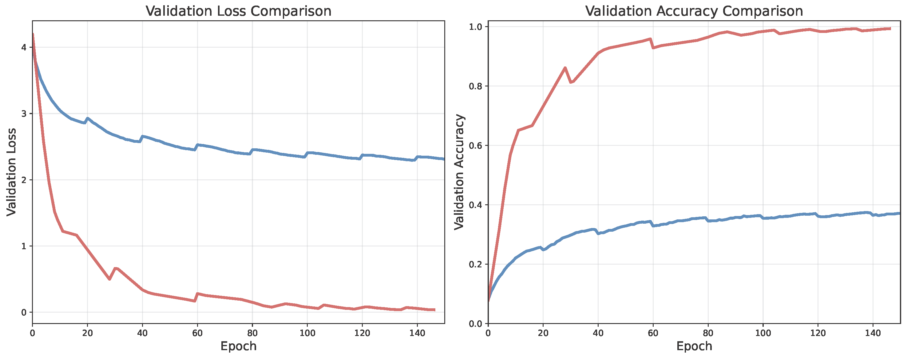
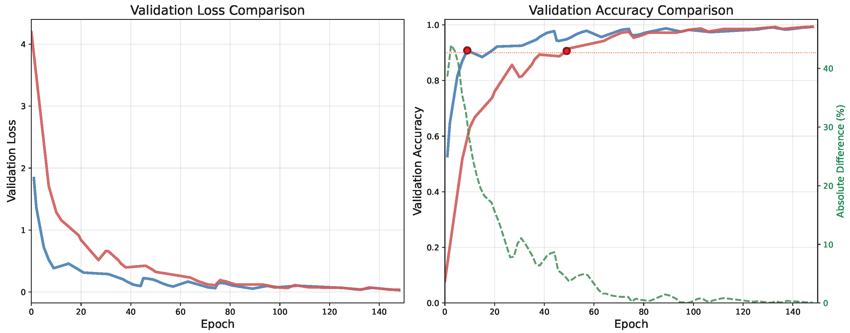
We conducted an ablation experiment to evaluate whether our constraint update mechanism benefits from using an LSTM cell over a simpler RNN cell. While the main experiments use LSTM-based updates, we performed a basic hyperparameter search for the RNN variant, adjusting learning rate, embedding dimension, batch size, and number of iterations. Across all runs, the RNN remained unstable and failed to exceed 40% validation accuracy. When using the same hyperparameters as the LSTM model (for a direct comparison), the RNN plateaued at 38.4% and exhibited higher validation loss.
Figure A1 shows the validation accuracy and loss during training for both variants. These results confirm the advantage of using more expressive update mechanisms (such as LSTM) for modeling our geometric constraints.
Figure A1.
Comparison of LSTM- and RNN-based constraint update mechanisms. The LSTM achieves higher validation accuracy and lower loss (red). The RNN variant achieves only 38.4% accuracy and performs worse in terms of loss (blue).
Figure A1.
Comparison of LSTM- and RNN-based constraint update mechanisms. The LSTM achieves higher validation accuracy and lower loss (red). The RNN variant achieves only 38.4% accuracy and performs worse in terms of loss (blue).
Appendix B. Embedding Visualization for the GNN in 3D
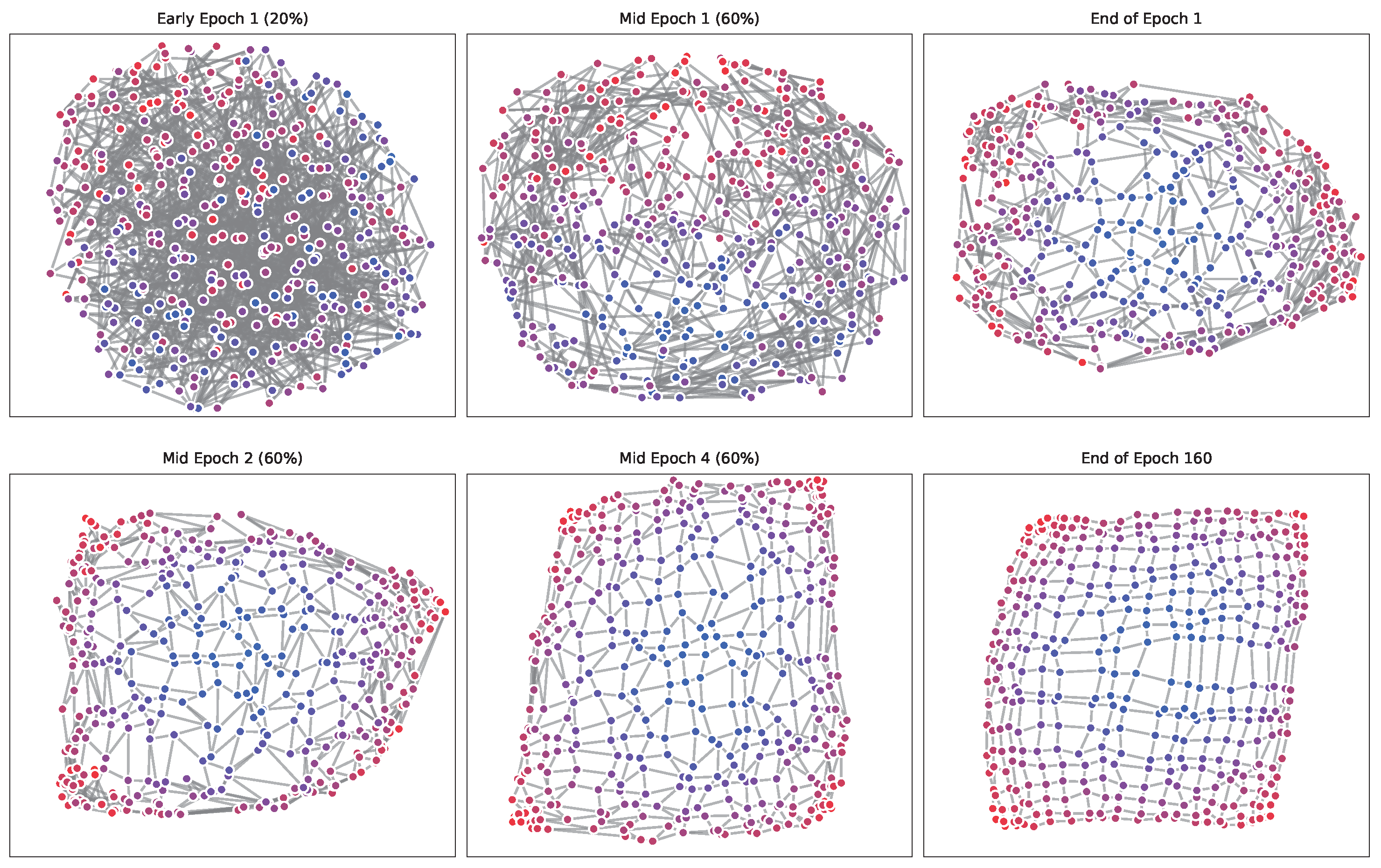
As mentioned in
Section 4.3, the static embeddings of individual points self-organize into a grid structure representing their spatial relationships. This section provides 3D visualizations to complement the 2D projections shown in the main text.
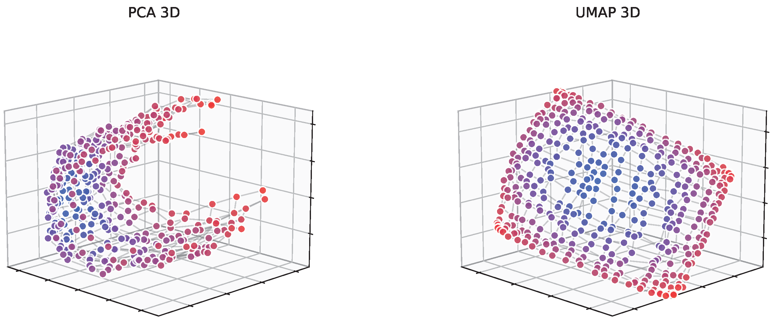
Figure A2 shows 3D projections of the learned embeddings using both UMAP and PCA methods. From the UMAP projections, we observed that during training, randomly initialized embeddings evolve from a single spherical cluster, which later unfolds into a U-shaped surface and finally converges to a flat 2D surface.
In contrast, the PCA 3D visualization remains a curved “cup” or “bell” shape rather than the flat plane observed with UMAP even after full training. Thus the embeddings lie on a curved surface in the high-dimensional space rather than in a flat plane.
Figure A2.
Three-dimensional projections of static point embeddings from 128-dimensional space using PCA (left) and UMAP (right). PCA reveals a curved “cup”- or “bell”-shaped structure, while UMAP projects them onto a flatter surface that more clearly shows the 2D grid organization. Colors indicate distance from grid center.
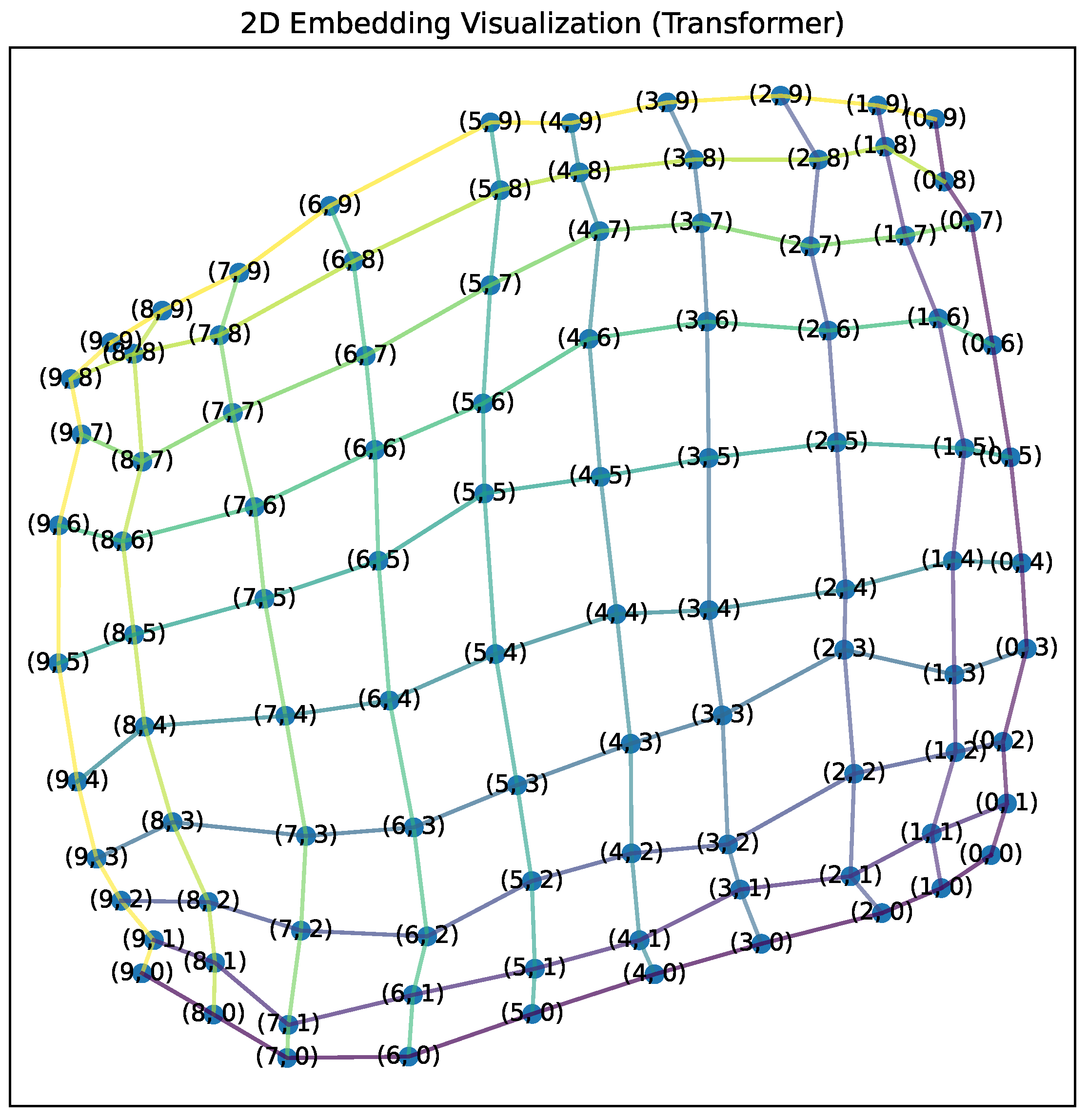
Figure A3.
Two-dimensional projections of static point embeddings from 128-dimensional space using PCA (left) and UMAP (right). PCA shows a curved, warped structure while UMAP better preserves the regular grid connectivity. Lines show spatial adjacency relationships from the original 20 × 20 grid. Colors indicate distance from grid center.
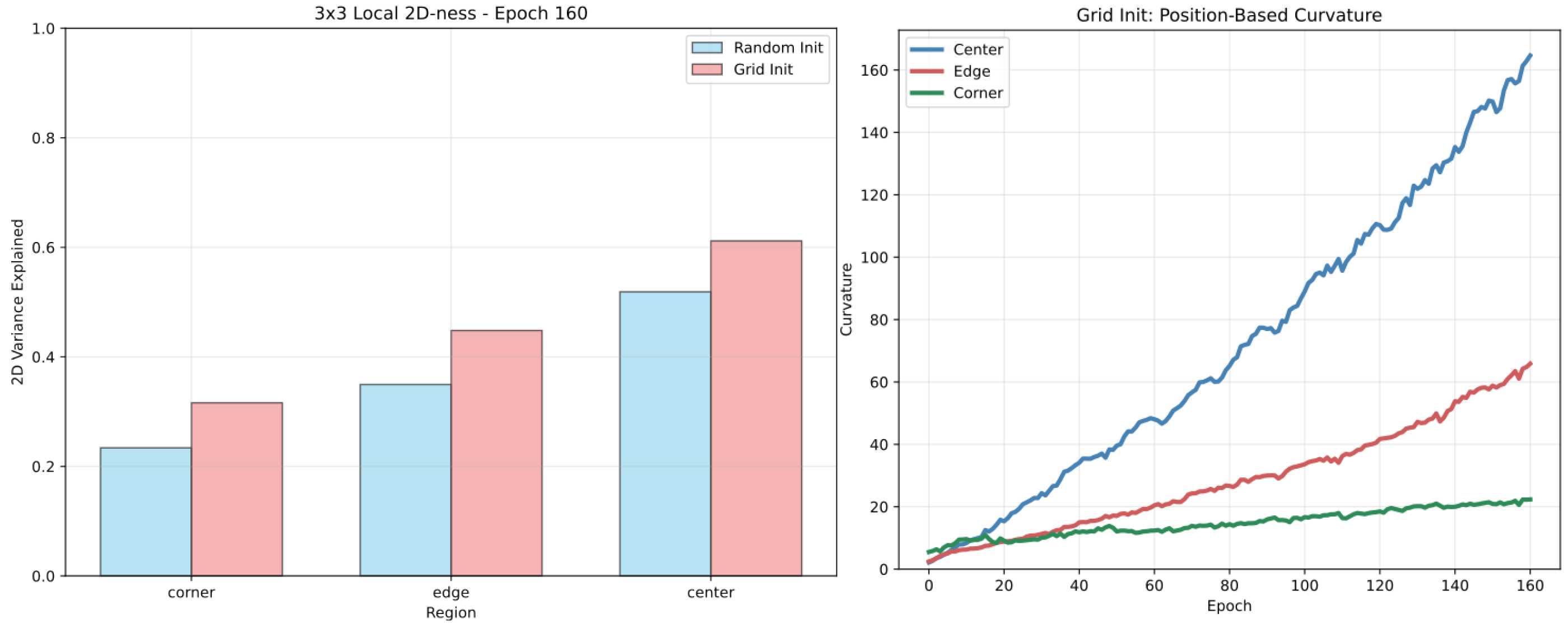
To further characterize the geometric evolution of the embedding space, we measure local curvature and local dimensionality throughout training (
Figure A4).
Curvature is computed in the 3D PCA projection using an eigenvalue-based method that quantifies deviation from local planarity within small neighborhoods. Specifically, we compute the local covariance matrix
of each neighborhood and define curvature as the ratio between the smallest and largest eigenvalues:
where
and
are the smallest and largest eigenvalues of
C, and
is a small constant added for numerical stability.
In the case of random initialization, curvature starts relatively high and fluctuates. In contrast, curvature under grid initialization starts near zero but increases steadily over time, eventually reaching levels similar to the random case. This indicates that even when training begins from a perfectly planar manifold, the resulting structure develops nontrivial curvature as training progresses. In parallel, we evaluate local 2D-ness, defined as the variance explained by the top two principal components in spatial subgrids. This captures how locally planar the embedding remains. Together, these metrics provide complementary views on how spatial structure and geometric complexity evolve, and how these differ across initialization strategies.
Figure A4.
Curvature and local 2D-ness during training for random vs. grid initialization. Right: Mean curvature over training time and by spatial region. Curvature is computed in the 3D PCA projection using a local neighborhood eigenvalue method, and it reflects how much local patches deviate from planarity. The rising curvature over time corresponds to the emergent cup-like shape seen in 3D PCA plots. Left: 2D-ness, measured as the fraction of variance explained by the top 2 PCA components in spatial subgrids.
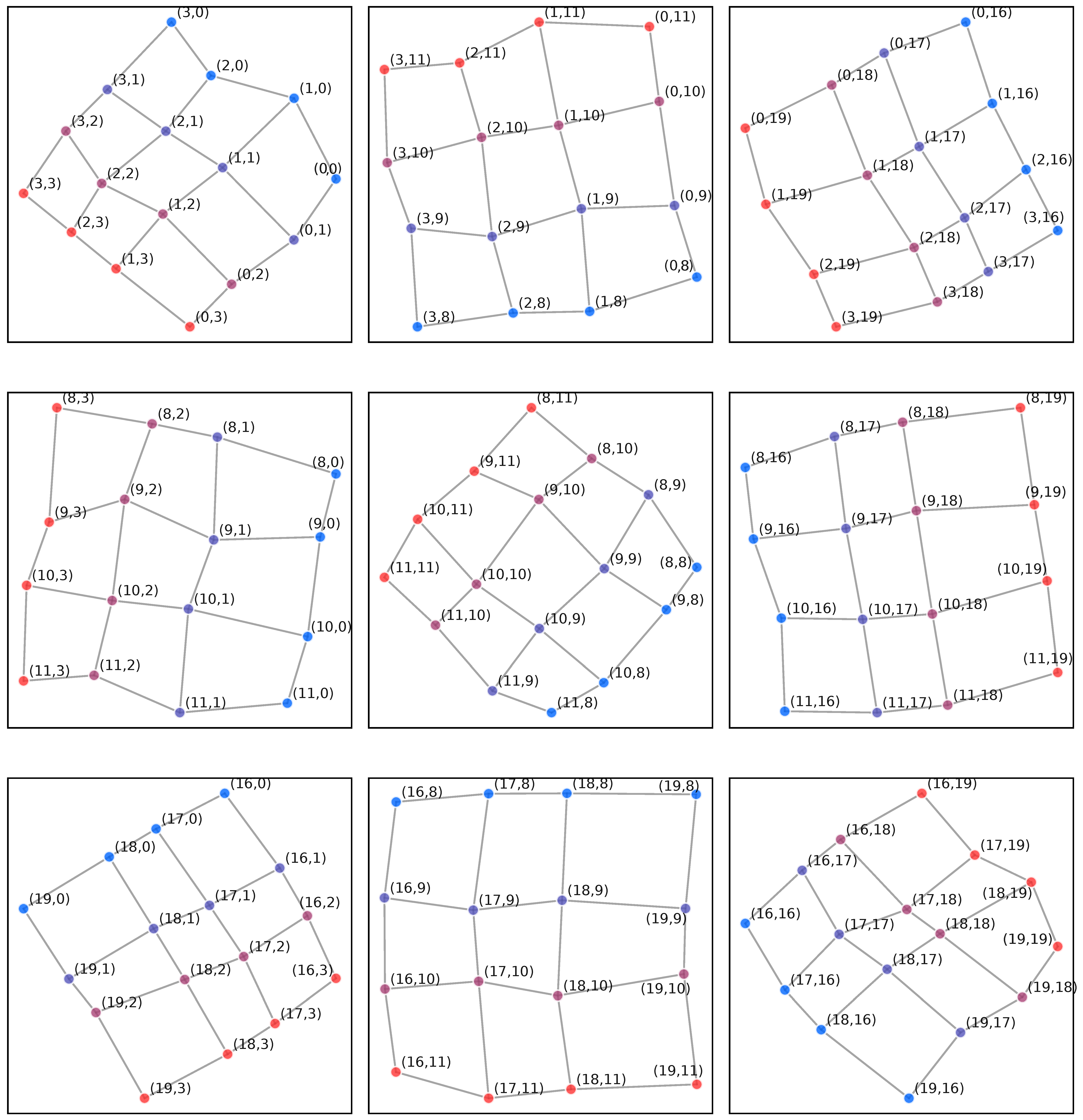
Figure A5 demonstrates that when examining 4 × 4 subregions of the 20 × 20 grid, PCA projections reveal well-organized local grid structures. This visualization technique shows that the embeddings maintain locally linear relationships within smaller regions, even though the global structure exhibits curvature.
Figure A5.
PCA projections of representative 4 × 4 subregions from the 20 × 20 grid embeddings, selected from corners and center areas for complete coverage. Local grid structure is well-preserved across all regions. While global embedding organization exhibits curvature (
Figure A2), these local neighborhoods maintain linear spatial relationships.
These visualizations confirm that the model successfully learns to embed spatial relationships in its high-dimensional representation, with the embeddings organized on a curved surface that preserves local neighborhood structure.
Figure A6 shows the distribution of variance across PCA components at different training stages and initialization methods. When training from random initialization, the first two components are most prominent at early stages (10 epochs). After full training (200 epochs), the variance spreads across approximately the first five components.
Training from precise grid initialization shows a different pattern. After 200 epochs, the first two components remain most prominent while the model utilizes additional dimensions, contrasting with the pure grid initialization baseline which concentrates variance primarily in two dimensions.
This analysis reveals how the usage of the embedding dimensions evolves during training and how initialization strategy affects the final embedding structure.
It also highlights the advantage of UMAP for our setup. UMAP offers a more accurate visualization of the learned grid structure than PCA. PCA is a global linear method and can distort local relationships when the embedding manifold becomes curved or non-planar, often placing distant points close together in projection. UMAP, by contrast, is a locally nonlinear method that better preserves neighborhood structure. This makes it more effective at representing the underlying grid organization when it becomes embedded in a non-planar, high-dimensional space.
Figure A6.
PCA component variance distribution across training conditions. (Top left) random initialization baseline. (Top right) after 200 epochs from random initialization, most variance spreads across approximately 5 components. (Bottom left) early training (10 epochs from random) shows the first 2 components are more prominent. (Bottom right) after 200 epochs from precise grid initialization, variance utilizes more dimensions than baseline but less prominently than random initialization training.
Appendix E. Chain-of-Thought Training
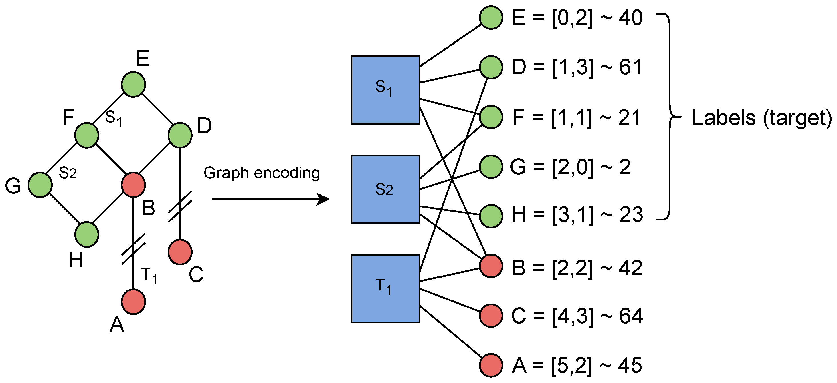
In order to train the Transformer to produce a chain-of-thought which assigns the variables incrementally, we implemented a simple solver which logs its steps and the resulting logs are used for imitation. The solver first orders the constraints according to a DAG mentioned in
Section 3.1 and then resolves the constraints one by one, starting from the root constraints. As the solver traverses the DAG, it logs the constraint of a given node, the values of already assigned variables within the constraint, and lastly the computed values for the remaining variables. We also include few keywords into the log which delimit the provided information. An example of the log for a random problem is shown below:
TRANSLATION ( 1 0 2 3 ) , TRANSLATION ( 5 4 7 6 ) , SQUARE ( 8 7 9 3 ) , SQUARE ( 11 8 10 3 ) , TRANSLATION ( 8 7 12 3 ) ; fixed 0 = #696 , 1 = #617 , 2 = #978 , 4 = #577 , 5 = #498 , 6 = #731 ; Solution begins ; Con TRANSLATION ( 5 4 7 6 ) ; Known 5 = #498 , 4 = #577 , 6 = #731 ; Impl 7 = #652 ; Con TRANSLATION ( 1 0 2 3 ) ; Known 1 = #617 , 0 = #696 , 2 = #978 ; Impl 3 = #1057 ; Con SQUARE ( 8 7 9 3 ) ; Known 7 = #652 , 3 = #1057 ; Impl 8 = #462 , 9 = #867 ; Con SQUARE ( 11 8 10 3 ) ; Known 8 = #462 , 3 = #1057 ; Impl 11 = #247 , 10 = #842 ; Con TRANSLATION ( 8 7 12 3 ) ; Known 8 = #462 , 7 = #652 , 3 = #1057 ; Impl 12 = #867 ; Solution ends
Variables are expressed by a number (1, 2, 3, etc.) and individual points are expressed with point ID with a # symbol in front (#696, #617, etc.). The input has two parts: a problem statement and a solution. We train on the whole input, but exclude the problem statement from the computation of the loss. For validation, we include only the problem statement. The keyword Con marks the selected constraint, Known marks the known variables which appear in the selected constraint with their values, and Impl marks the newly deduced variables with their values.
Appendix F. Test-Time Scaling and Iteration Analysis
This section analyzes model behavior across different iteration counts and resampling strategies, supporting the test-time scaling results presented in
Table 1.
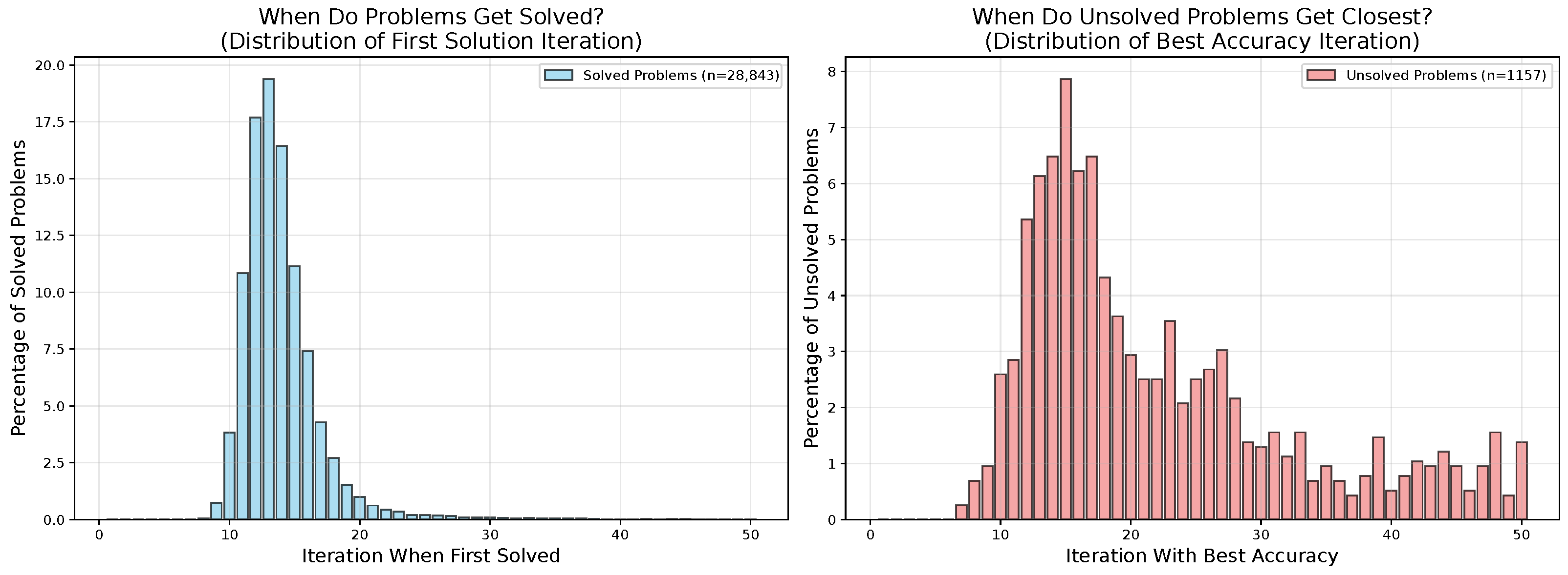
Figure A9 shows the distribution of iterations when variables are correctly assigned for the first time (left) and when unsolved problems achieve their best point accuracy (right) using single resampling. Most problems that can be solved are resolved within the first 15 iterations, with a long tail extending to 50 iterations. For unsolved problems, the peak occurs around iterations 10–15, though substantial numbers of problems achieve their best accuracy at later iterations, indicating that additional computation can still provide benefits.
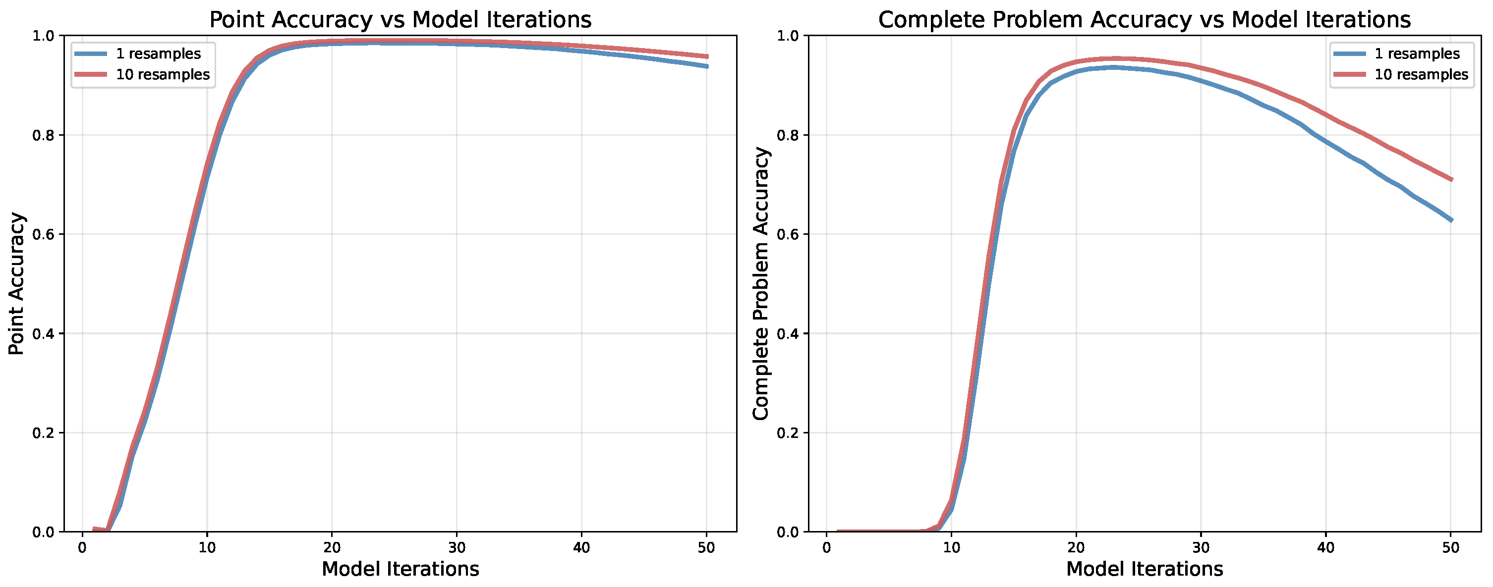
Figure A10 demonstrates how accuracy evolves with iteration count for both single and multiple resampling strategies. Both point and complete problem accuracy peak around iterations 23–25, then decline with further iterations. This indicates that while some individual problems benefit from extended computation (as shown in
Figure A9), increasing iterations beyond 25 breaks more already-solved instances than it helps, resulting in net performance degradation.
Multiple resamples provide consistent benefits across all iteration counts, with optimal performance occurring in the 23–25 iteration range for both strategies.
These results explain why increasing iterations from 15 to 23 improves complete accuracy and why the “Best” oracle configuration achieves higher performance by selecting optimal iteration counts per problem.
Figure A9.
When problems reach solution during inference. Left: distribution of first solution iteration for successfully solved problems. Right: iteration when unsolved problems achieve their highest point accuracy.
Figure A9.
When problems reach solution during inference. Left: distribution of first solution iteration for successfully solved problems. Right: iteration when unsolved problems achieve their highest point accuracy.
Figure A10.
Model performance across iteration counts with single resampling (blue) and 10 resamples (red). Both point accuracy and complete problem accuracy peak around iterations 23–25, then decline. Multiple resampling provides consistent benefits across all iteration counts.
Figure A10.
Model performance across iteration counts with single resampling (blue) and 10 resamples (red). Both point accuracy and complete problem accuracy peak around iterations 23–25, then decline. Multiple resampling provides consistent benefits across all iteration counts.
Appendix G. Scaling the Size of the Grid
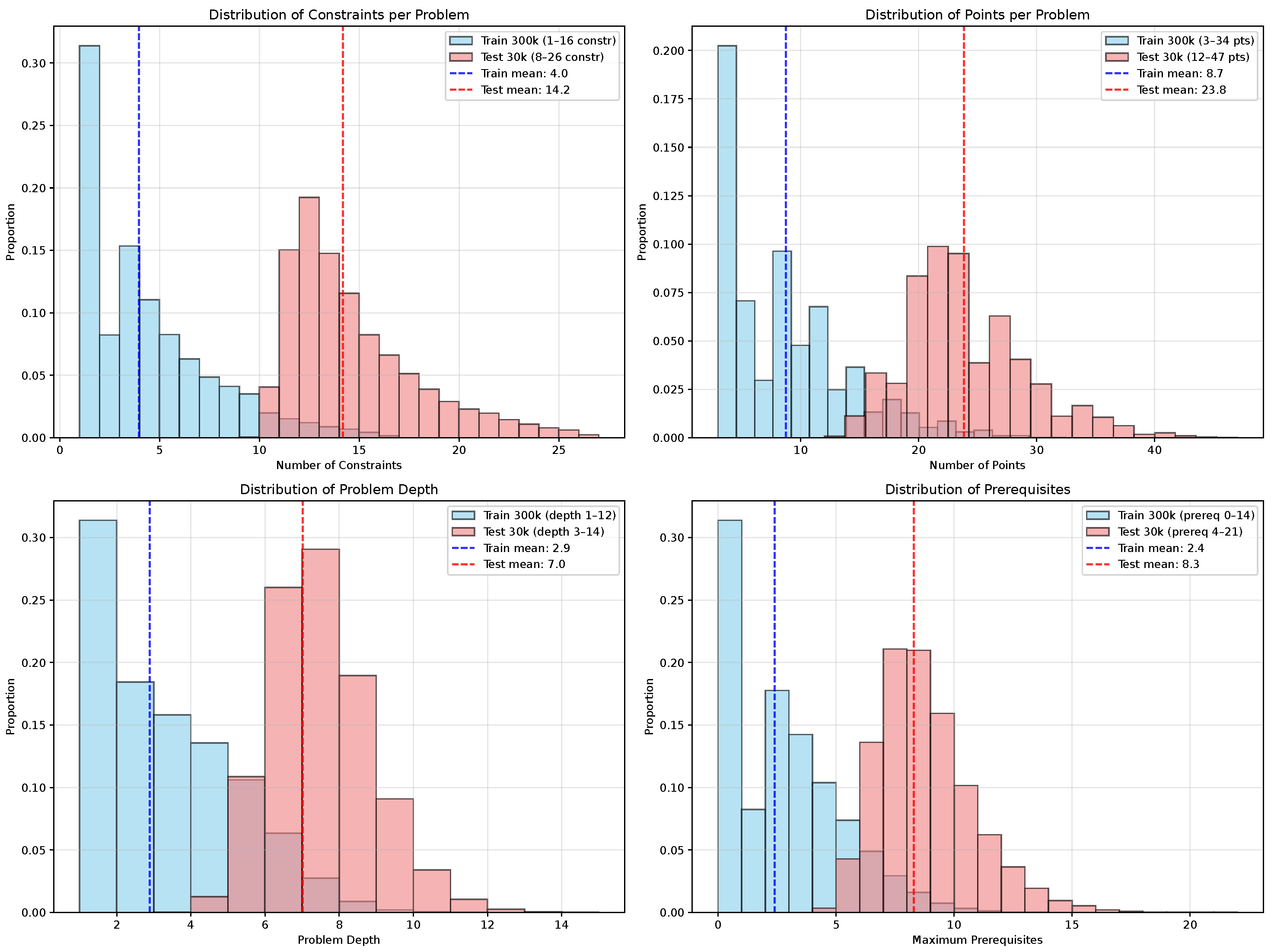
To get a sense of how the sample complexity depends on the size of the grid, we trained several models on different sizes of the grid and different amount of training samples. To achieve faster training, we conducted these experiments with problems which contained only two types of constraints (S and T).
The problem generator mentioned in
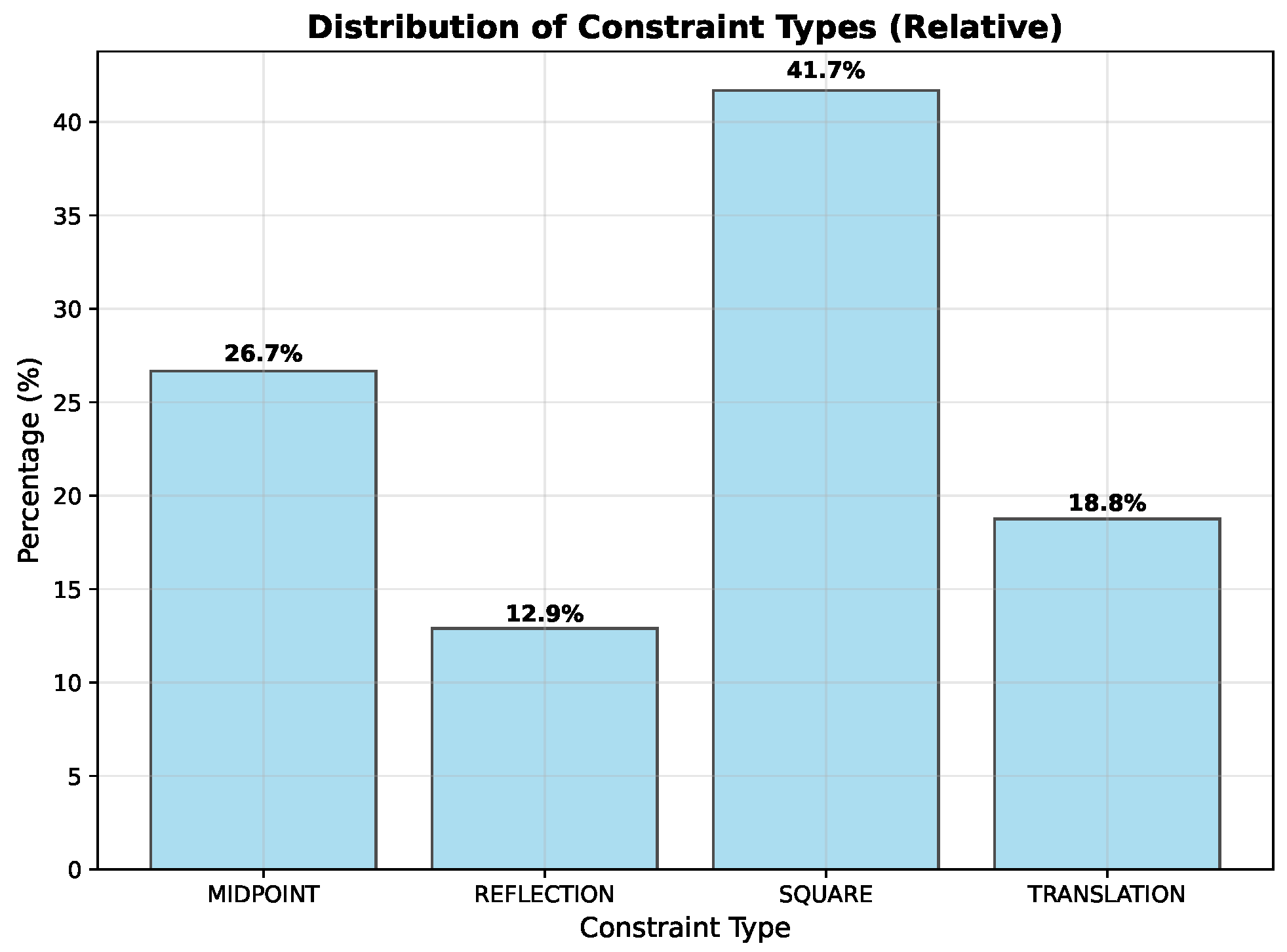
Section 3.1 produces problems which have, on average, around four constraints. Both types of constraints (
S and
T) are sampled with equal probability. Therefore, we can assume that an average problem has two constraints of type
S (which are determined by two points) and two constraints of type
T (which are determined by three points). If we denote the number of points on the side of the grid by
n, then we can estimate the number of unique problems in an
-size grid to be
. There are
possible point positions and we independently sample six points for two constraints of type
T and four points for two constraints of type
S, together yielding
possibilities, each of which determines one instance. This number should be viewed as an upper bound because it ignores the fact that constraints can share variables.
To test the dependence of the validation accuracy on the grid size and number of training samples, we use the following values of n: 10, 20, 30, 40, 50, 60, 70, and 80. This results in the following number (after rounding the exponent to the nearest integer) of possible problems for each n, respectively: , , , , , , , and .
The sizes of the training set for each grid size are in the range from 5k to 800k. The relationship between the validation accuracy, the grid size, and the size of the training set can be seen in
Figure A11. In the same Figure (right), we plot the relationship between the grid size and sizes of the training set for which the validation accuracy exceeded
.
Figure A11.
Scaling analysis for different grid sizes using simplified problems with only Square and Translation constraints. Left: validation accuracy versus training set size for grids from 10 × 10 to 80 × 80 points. Right: sample complexity required to achieve 90% accuracy across different grid sizes.
Appendix H. More Examples of the Solution Process
This section provides additional examples of the iterative solution process to support the findings presented in
Section 4.5. While the main text focused on a single detailed example, these three instances demonstrate that the observed iterative refinement behavior is consistent across different problem configurations and constraint combinations.
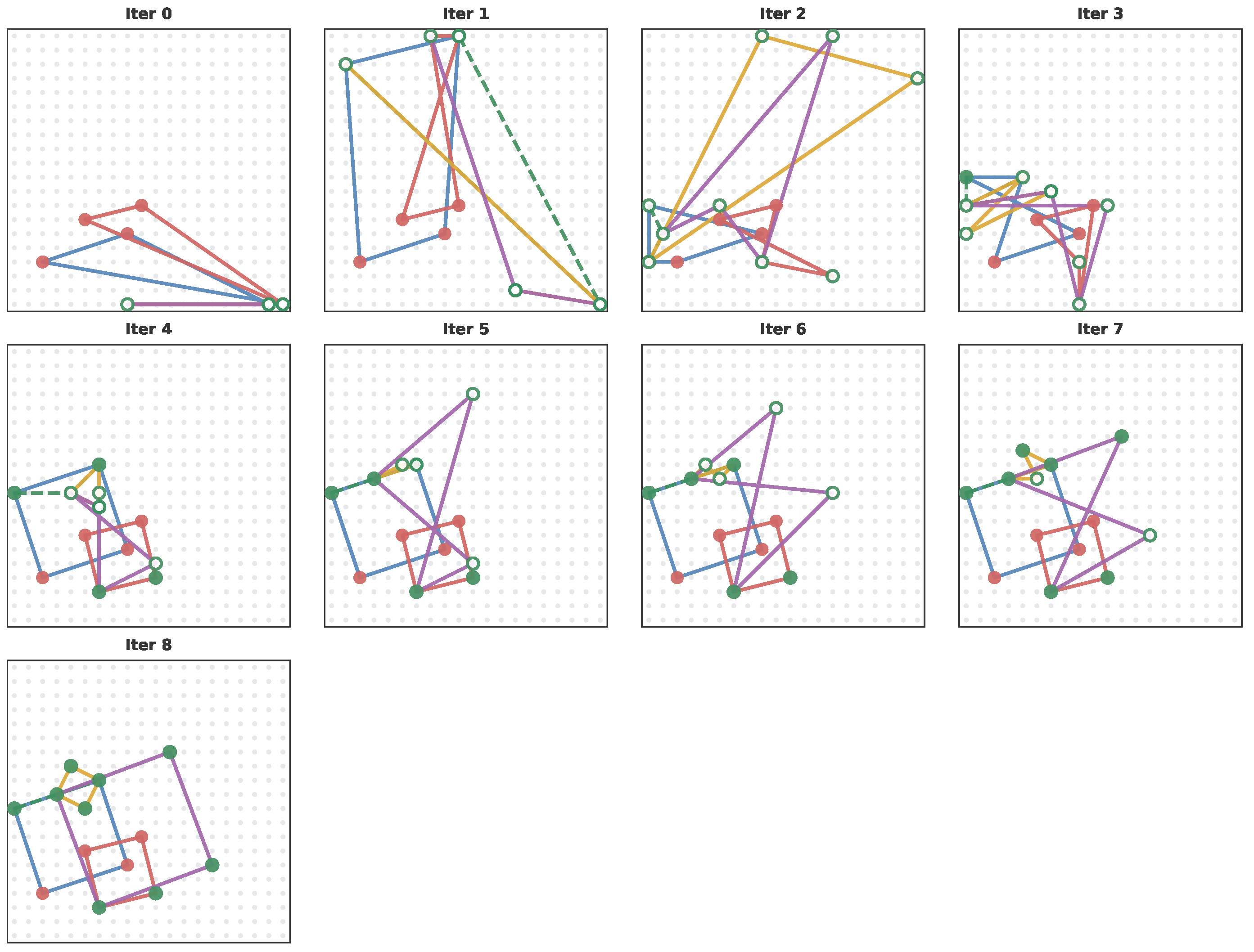
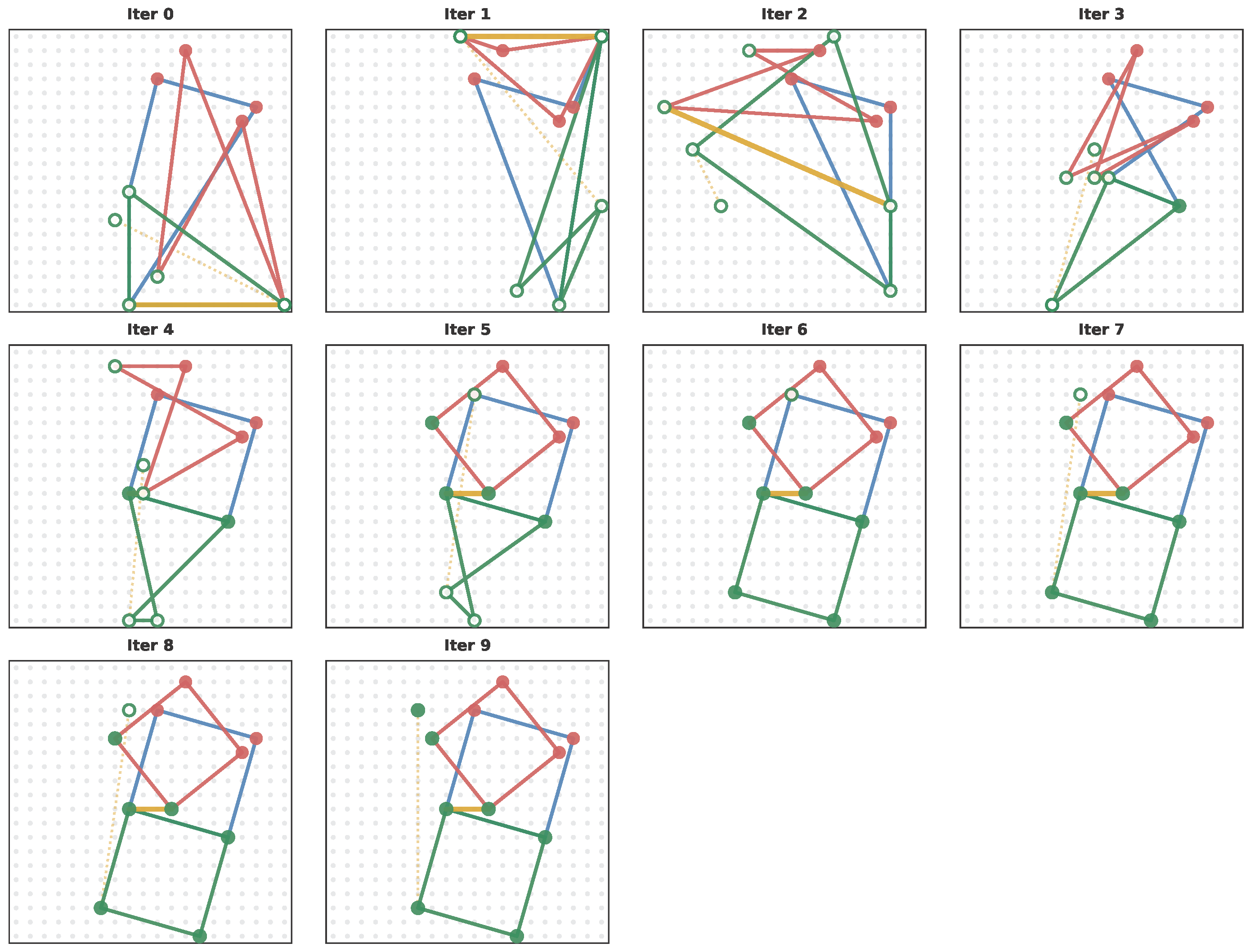
These examples cover three of the four constraint types in our CSP language, Midpoint (
M), Reflection (
R), and Square (
S), providing broader evidence for the model’s geometric reasoning capabilities. The instances shown in
Figure A12,
Figure A13 and
Figure A14 were selected primarily for visual clarity. Some generated problems place points in close proximity, obscuring the iterative dynamics when visualized.
Unlike the prominent example in the main text, we omit point labels to avoid visual clutter while still clearly showing the constraint relationships through colored lines (for the same reason, only problems with low constraint amount and depth are presented). Each figure shows how the model progressively constructs the hidden geometric configuration, with constraint satisfaction improving over iterations until convergence to the correct solution. These examples reinforce our core finding that the GNN employs a continuous optimization-like process to solve geometric constraint problems, moving point embeddings iteratively toward configurations that satisfy the given constraints.
In these visualizations, known points appear as fixed red markers throughout all iterations, while unknown points are shown as green markers that move as the model iterates. Unknown points appear as empty circles when incorrectly positioned and filled circles when they reach their correct locations. We display all iterations until final resolution. Different constraint types use distinct visual representations: Square constraints appear as full lines connecting all four vertices, Midpoint constraints use dashed lines forming a three-point chain, and Reflection constraints show full lines connecting the axis points with less visible dotted lines connecting the reflected point pairs.
Figure A12.
Problem with five constraints: four Squares and one Midpoint. The Midpoint constraint (dashed green line) coincides with the top side of the blue Square (two vertices of the smallest Square). Point colors denote known (red) and unknown (green) variables. Line colors are used to differentiate between the constraints in the problem. If a green point is empty, it is not in the right position yet.
Figure A13.
Problem with four constraints: three Squares and one Reflection. The two leftmost points are reflected across the axis formed by the yellow line segment. Point colors denote known (red) and unknown (green) variables. Line colors are used to differentiate between the constraints in the problem. If a green point is empty, it is not in the right position yet.
Figure A14.
Problem with six constraints: two Squares, three Midpoints, and one Reflection. One Midpoint is less visible in the final solution because it is both a common vertex of both Squares and simultaneously the midpoint of two different Midpoint constraints. The orange line segment provides the Reflection axis. Point colors denote known (red) and unknown (green) variables. Line colors are used to differentiate between the constraints in the problem. If a green point is empty, it is not in the right position yet.
Appendix I. Constraint Embedding Analysis
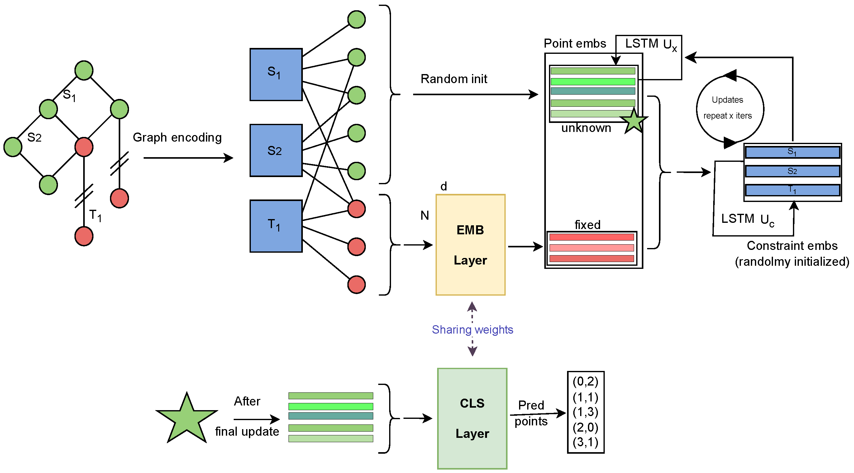
We analyze the information encoded in constraint embeddings produced by the GNN during its iterative process. These embeddings are updated using information from both fixed and unknown points.
Appendix I.1. Constraint Type Classification
We tested whether constraint embeddings encode their constraint type by training a simple MLP classifier (two linear layers with ReLU) on the embeddings. The classifier achieved over
accuracy predicting constraint types.
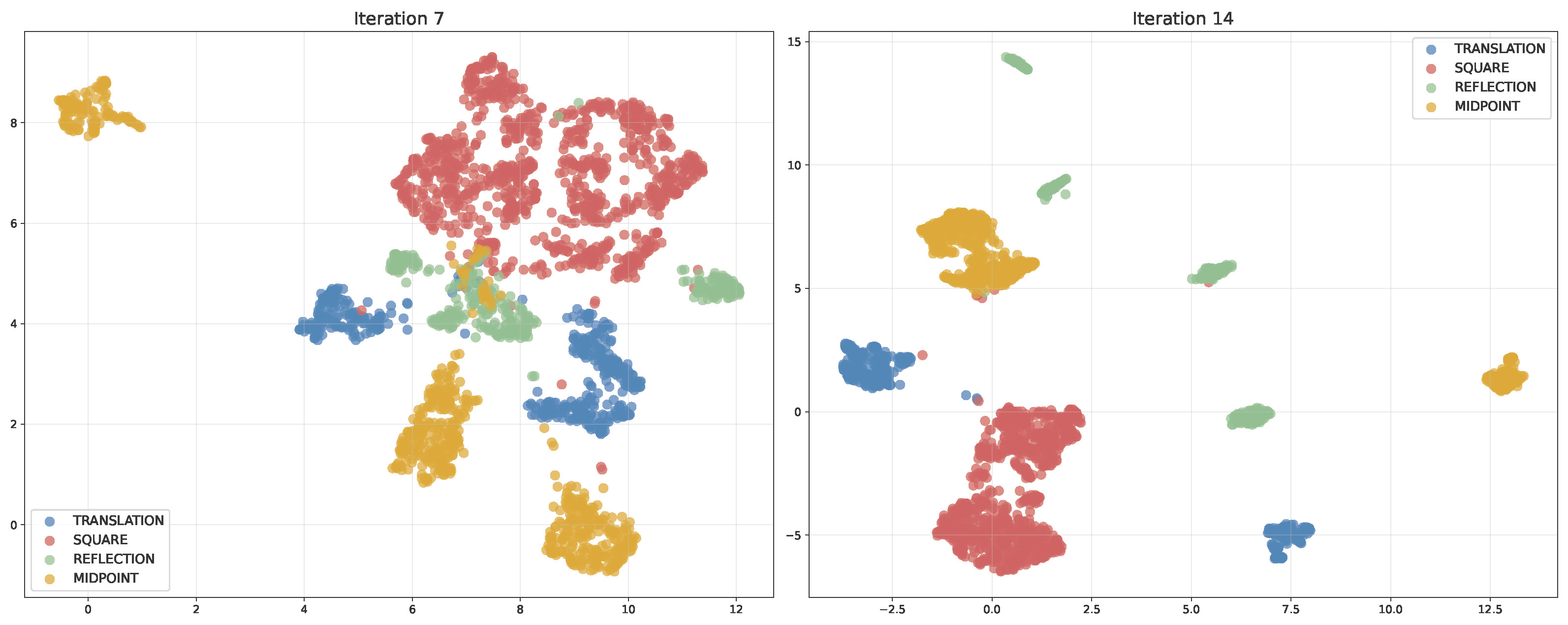
Figure A15 shows the clear separation between constraint types in the projected embedding space using UMAP.
Figure A15.
Constraint embedding clusters after 8 and 15 iterations, projected using UMAP. Different constraint types form distinct clusters, with subclusters reflecting geometric properties and network biases.
Figure A15.
Constraint embedding clusters after 8 and 15 iterations, projected using UMAP. Different constraint types form distinct clusters, with subclusters reflecting geometric properties and network biases.
Each constraint type exhibits subclustering patterns that reflect geometric properties, network processing biases, and some generator design choices. Square constraints form subclusters based on side orientation relative to the grid (parallel versus diagonal orientations). Midpoint constraints cluster according to which variable is unknown: the Midpoint itself or one of the endpoint variables. Reflection constraints show four subclusters corresponding to reflection axis orientation: two for axes parallel to grid edges and two for diagonal axes. Translation constraints exhibit order-dependent clustering based on which variables in the constraint are unknown—specifically whether variables or are unknown—revealing network bias toward variable ordering. Note that we identified fewer distinct subclusters than the maximum possible number, as some potential subclusters appeared very close in the embedding space.
These patterns indicate that constraint embeddings encode both geometric properties and structural biases from the network’s processing order. As discussed in
Section 3.1, our generator creates problems requiring unique solutions through specific dependency structures, which may contribute to these ordering biases. Future work could explore making constraints invariant to variable permutations.
Appendix I.2. Constraint Satisfaction Prediction
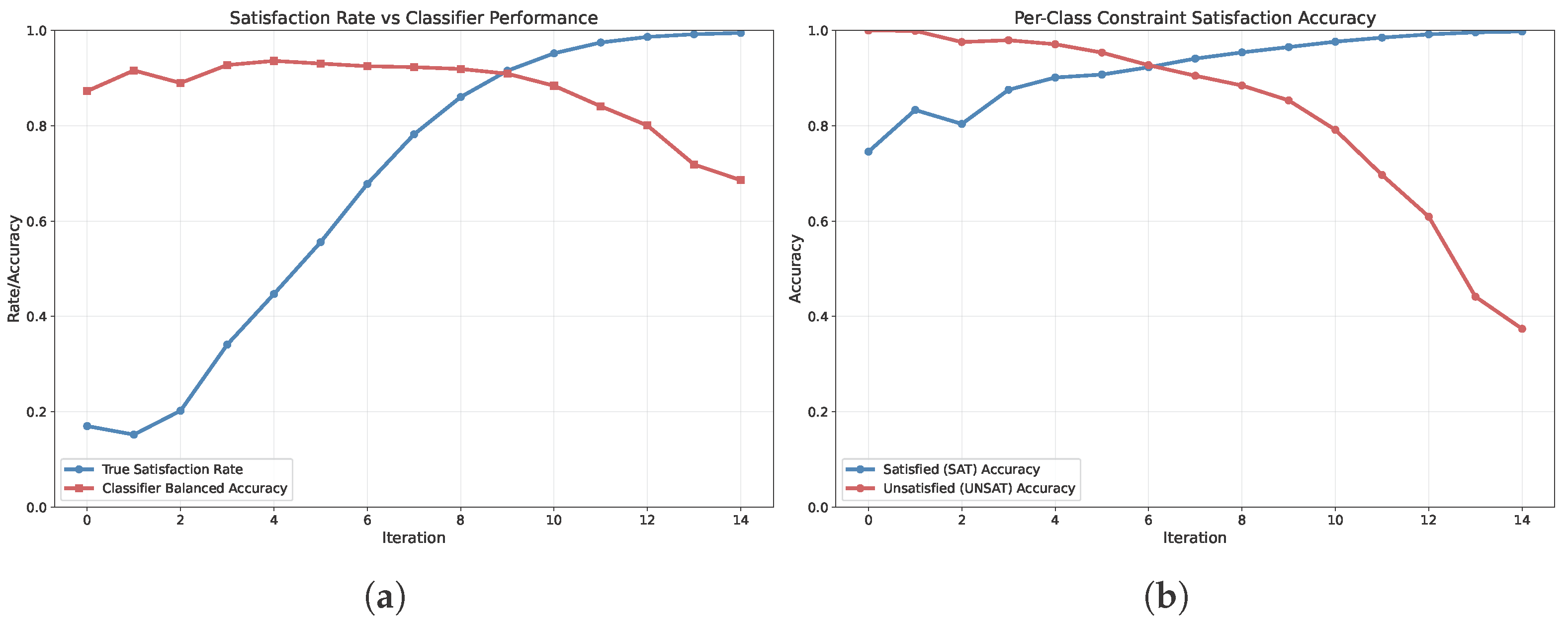
We trained an MLP classifier to predict whether individual constraints are satisfied at each iteration. Using our 30k test dataset, we annotated constraint satisfaction status after each iteration up to 15 iterations and split the data: for training, for validation, and for testing. We made sure that the training data had balanced classes.
For early iterations, the classifier achieved over
accuracy. However, performance degraded for higher iterations, as shown in
Figure A16. The model increasingly predicted “satisfied” for most constraints as iteration count increased, regardless of actual satisfaction status.
Figure A16.
Constraint satisfaction prediction accuracy across iterations. (a) True satisfaction rate versus classifier-balanced accuracy. (b) Per-class accuracy showing the model’s bias toward predicting “satisfied” at higher iterations.
Figure A16.
Constraint satisfaction prediction accuracy across iterations. (a) True satisfaction rate versus classifier-balanced accuracy. (b) Per-class accuracy showing the model’s bias toward predicting “satisfied” at higher iterations.
Appendix I.3. Temporal Information Encoding
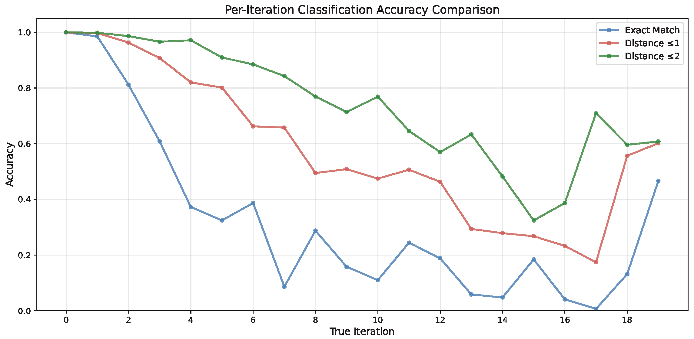
We investigated whether constraint embeddings encode iteration number by training an MLP to predict the current iteration from constraint embeddings. Results using 20 iterations are shown in
Figure A17.
Figure A17.
Accuracy of predicting iteration number from constraint embeddings. Exact match accuracy (blue), and when allowing distance 1 (orange) and distance 2 (green) tolerance. The model accurately predicts early iterations (≤4) but becomes less reliable for higher iteration counts.
Figure A17.
Accuracy of predicting iteration number from constraint embeddings. Exact match accuracy (blue), and when allowing distance 1 (orange) and distance 2 (green) tolerance. The model accurately predicts early iterations (≤4) but becomes less reliable for higher iteration counts.
The classifier achieves high accuracy for early iterations (≤4) but becomes less reliable for higher iteration counts. When allowing tolerance (predicting within 1–2 iterations of the true value), accuracy clearly improves. This indicates that constraint embeddings do encode temporal information, though with decreasing precision for later iterations.
When trained on higher maximum iteration counts, the predictor defaults to the final iteration class for later iterations, suggesting it learns a coarse ‘early’ vs ‘late’ distinction rather than precise temporal positioning. This may be due to the original GNN not being exposed to longer sequences during training.
These findings demonstrate that constraint embeddings encode rich information about constraint types, geometric relationships, satisfaction status, and temporal progression, providing more insight into the model’s internal reasoning process.
Appendix J. Evolution of Constraints Under UMAP Projection
Unlike earlier visualizations which involved the interpretation of classification outputs in a precise 2D grid, this analysis focuses on how the embedding space itself organizes geometric reasoning. We use UMAP to project the point embeddings: both the static embeddings from the shared embedding layer and the evolving embeddings of unknown points during inference into 2D space. These projections are not tied to the output logits or grid structure, but purely reflect how the network shapes its internal representation geometry.
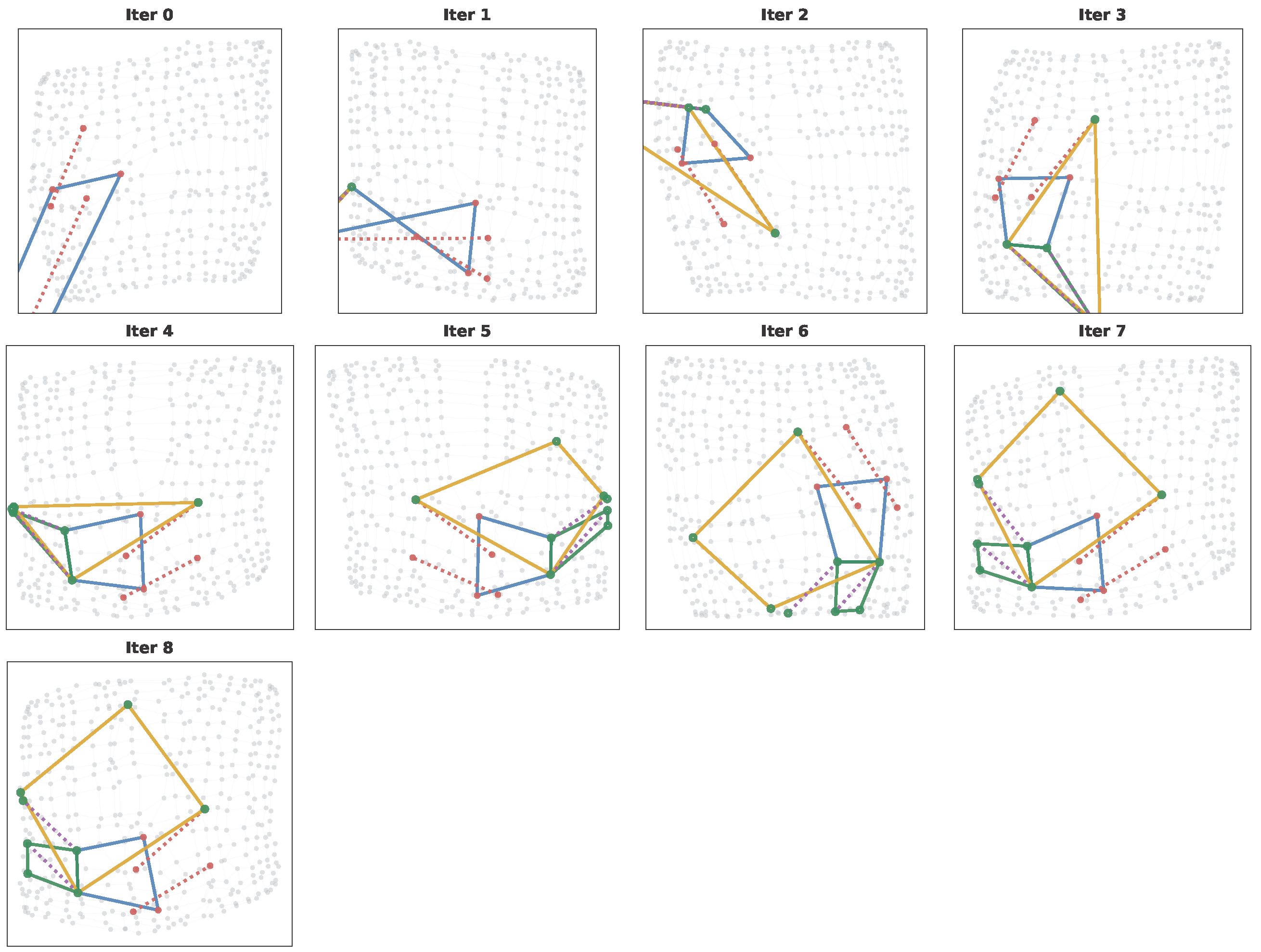
To visualize the reasoning dynamics, we perform the projection independently at each inference iteration. We then connect the points that participate in the same constraint using the same logic as in earlier visualizations in the precise 2D grid (i.e., if there is a line segment between points A and B in the shape for the given constraint, we add the segment to the projected image). This allows us to track how spatial relationships emerge and evolve directly in embedding space, without reference to grid positions or decoded predictions.
At the start of inference, the embeddings of unknown points are randomly initialized and lie far from the structured region formed by the fixed (grid) embeddings. During inference, especially within the first five iterations, these points are pulled into the manifold shaped by the fixed points of the grid, forming a coherent geometric configuration. This initial phase is clearly visible in the UMAP projections, reflecting the alignment of unknown embeddings with the learned spatial structure.
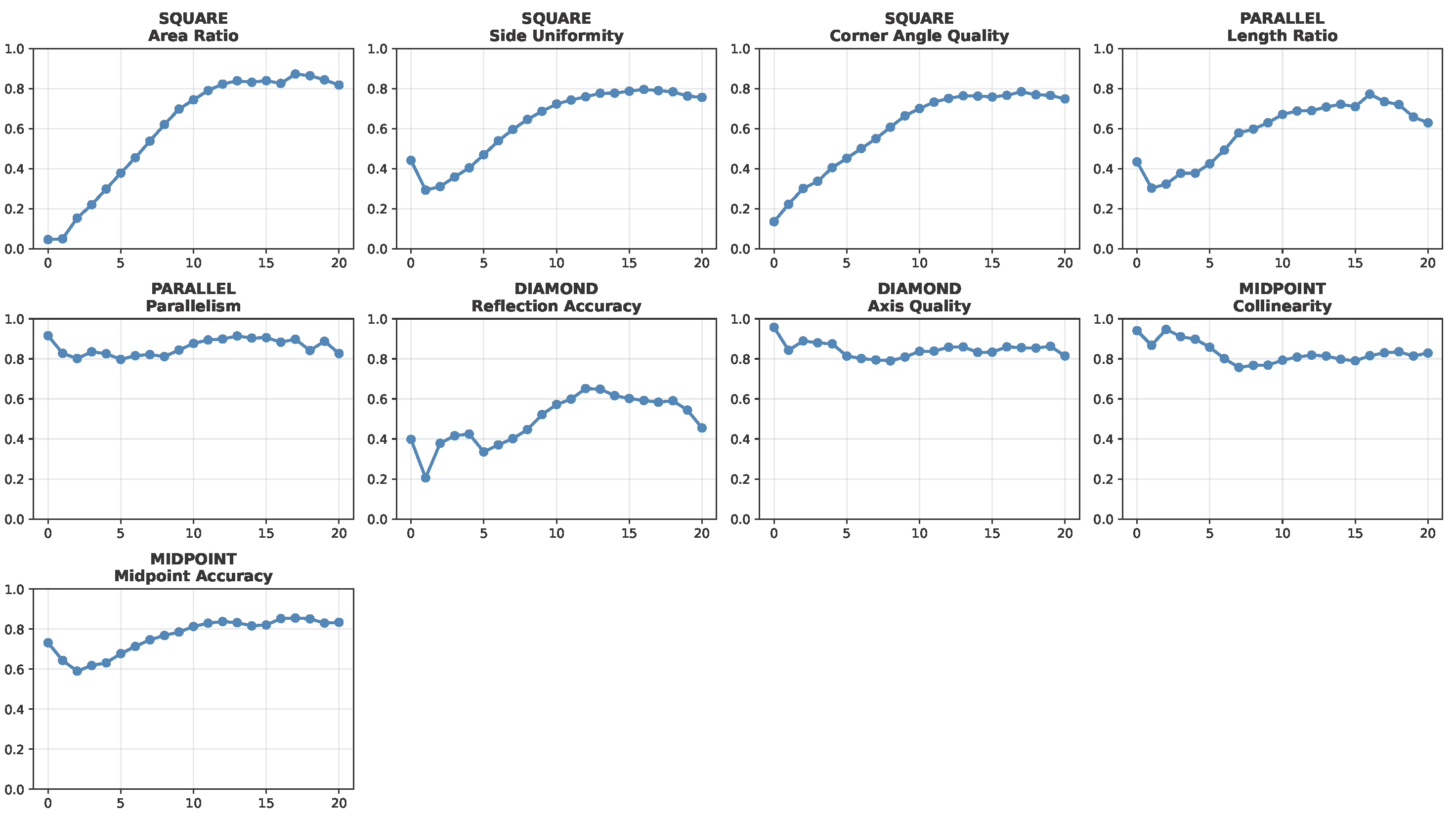
We also tried to quantify these dynamics by computing several geometric metrics over the UMAP projections at each iteration. We computed a set of nine normalized metrics, each producing a score in , where indicates perfect satisfaction of a geometric property. These are grouped by constraint type:
Figure A18.
Constraint- based visualization of the UMAP projection of point embeddings across inference iterations for a simple problem. Each panel shows the embedding space at one iteration. Points are connected based on constraint structure. Point colors denote known (red) and unknown (green) variables. Line colors are used to differentiate between the constraints in the problem.
Figure A19.
UMAP projections over inference time for a more complex instance with 13 constraints. Despite projection being performed independently per iteration, the geometric structure of the figure consistently emerges in embedding space. Constraint-based connections reveal progressive organization of the unknown points. Point colors denote known (red) and unknown (green) variables. Line colors are used to differentiate between the constraints in the problem.
Figure A20 shows the average value of these metrics per constraint type and iteration. The results indicate that geometric regularities emerge over time in the embedding space (even though no supervision is provided on these properties). This supports the interpretation that the network builds and organizes internal geometry as part of its reasoning process, and that UMAP is suited to uncover this structure (it would not work in the original dimension or under PCA).
Figure A20.
Evolution of geometric metrics computed on UMAP projections of point embeddings. Left: parallelism (axis alignment) across similar constraint types. Middle: average per-point movement across iterations (embedding consistency). Right: directional coherence for constraints of the same type (direction quality). All metrics are averaged across test instances and grouped by constraint type.
