Article

A Dynamic Hypergraph-Based Encoder–Decoder Risk Model for Longitudinal Predictions of Knee Osteoarthritis Progression

by
John B. Theocharis
,
Christos G. Chadoulos
*,† and
Andreas L. Symeonidis
Department of Electrical & Computer Engineering, Aristotle University of Thessaloniki, 54124 Thessaloniki, Greece
*
Author to whom correspondence should be addressed.
These authors contributed equally to this work.
Mach. Learn. Knowl. Extr. 2025, 7(3), 94; https://doi.org/10.3390/make7030094
Submission received: 8 July 2025 / Revised: 19 August 2025 / Accepted: 27 August 2025 / Published: 2 September 2025
(This article belongs to the Special Issue Advances in Machine and Deep Learning)

Abstract

Knee osteoarthritis (KOA) is a most prevalent chronic muscoloskeletal disorder causing pain and functional impairment. Accurate predictions of KOA evolution are important for early interventions and preventive treatment planning. In this paper, we propose a novel dynamic hypergraph-based risk model (DyHRM) which integrates the encoder–decoder (ED) architecture with hypergraph convolutional neural networks (HGCNs). The risk model is used to generate longitudinal forecasts of KOA incidence and progression based on the knee evolution at a historical stage. DyHRM comprises two main parts, namely the dynamic hypergraph gated recurrent unit (DyHGRU) and the multi-view HGCN (MHGCN) networks. The ED-based DyHGRU follows the sequence-to-sequence learning approach. The encoder first transforms a knee sequence at the historical stage into a sequence of hidden states in a latent space. The Attention-based Context Transformer (ACT) is designed to identify important temporal trends in the encoder’s state sequence, while the decoder is used to generate sequences of KOA progression, at the prediction stage. MHGCN conducts multi-view spatial HGCN convolutions of the original knee data at each step of the historic stage. The aim is to acquire more comprehensive feature representations of nodes by exploiting different hyperedges (views), including the global shape descriptors of the cartilage volume, the injury history, and the demographic risk factors. In addition to DyHRM, we also propose the HyGraphSMOTE method to confront the inherent class imbalance problem in KOA datasets, between the knee progressors (minority) and non-progressors (majority). Embedded in MHGCN, the HyGraphSMOTE algorithm tackles data balancing in a systematic way, by generating new synthetic node sequences of the minority class via interpolation. Extensive experiments are conducted using the Osteoarthritis Initiative (OAI) cohort to validate the accuracy of longitudinal predictions acquired by DyHRM under different definition criteria of KOA incidence and progression. The basic finding of the experiments is that the larger the historic depth, the higher the accuracy of the obtained forecasts ahead. Comparative results demonstrate the efficacy of DyHRM against other state-of-the-art methods in this field.

1. Introduction

Knee osteoarthritis (KOA) is one of the most prominent joint diseases affecting people around the world, with the majority of patients experiencing its onset at ages 60 or greater. The prominent factors that are considered to contribute the most in the onset and progression of the disease are (1) misalignments in bone structure and anatomy, either inherited (congenital) or acquired, (2) excess body weight which over time can considerably stress the knee joint, coupled with a general state of inactivity which, eventually weakens and diminishes the supporting musculature, and (3) advanced age [1], among others. The damage in the cartilage and surrounding tissues, induced by the condition, exposes the femoral and tibial bones to high friction forces during everyday movements, leading to a gradual denudation of the cartilage volume, and in more extreme scenarios, to complete exposure of the respective bone surfaces and to the development of bony protrusions in the form of osteophytes. The above consequences eventually result in substantial loss of quality of life in more severe cases, limiting the patients’ mobility in every-day tasks, and overall leading to a state of diminished general well-being [2].

1.1. Koa Incidence and Progression

A crucial component in accurately diagnosing KOA in patients is the examination and evaluation of imaging data in the form of knee X-rays and MRIs. Imaging biomarkers such as the Joint Space Width (JSW) and Joint Space Narrowing (JSN), the detection of cartilage denudation, and the identification of osteophytes’ presence are well established in the scientific literature and can facilitate the respective tasks of evaluating KOA severity [3].
Besides accurately diagnosing the presence of KOA, an equally critical task, from a clinical perspective, is the identification of the progression trajectory of the disease once it has been unequivocally detected. A robust progression prediction can allow the clinicians to chart an appropriate treatment course, tailored to the specific needs of the respective patient, in accordance to their particular progression profile.
Extending the available imaging data, the additional incorporation of generic demographic information may potentially yield a net positive effect in the predictive capabilities of the aforementioned models, since all the above variables constitute well-established risk factors that can directly or indirectly affect the future trajectory of KOA. Introducing variables such as age, Body Mass Index (BMI), and gender, as well as relevant medical information (i.e., past injury record), in the development of KOA risk models may potentially augment these models’ performance [4].
In the following, we provide a succinct review of the scientific literature landscape with regards to the aforementioned tasks of KOA incidence and progression prediction.
  • KOA Incidence: The main body of research in KOA identification and longitudinal prediction operates under the following directive: Given the patients’ data at an initial baseline time point, identify the presence and/or severity of the condition at a specific time point in the future. In [5], the authors develop a CNN architecture utilizing the Convolutional Block Attention Module (CBAM) [6] for automatic KL grade classification. Guan et al. [7] develop a series of deep learning models to identify the onset of the disease during a follow-up period of 48 months. A similar approach is adopted by the authors in [8], where T 2 maps are employed to diagnose radiographic KOA, while in [7], a series of deep learning models are developed and evaluated for the prediction of medial joint space loss at 48 months after the baseline visit. A Convolutional Variational Autoencoder (CVAE) was employed in [9] for the early detection of KOA incidence, within a short period of 24 months. An Adversarial Evolving Neural Network (AENN) was proposed by the authors in [10] for longitudinal grading of KOA severity. The authors in [11] develop a risk prediction Tool for Osteoarthritis Risk Prediction (TOARP) with the goal of producing estimates of KOA incidence over an 8-year period. The work in [12] evaluates a series of radiographic features to determine KOA incidence in patients with recently developed knee pain, within a time-frame of 5 years. Finally, in [13], a risk prediction model combining clinical, genetic, and biochemical risk factors is proposed to yield KL score predictions at regular points in the future.
  • KOA progression: With regards to the problem of progression modeling, the main task lies in identifying the progression patterns of clinical biomarkers, such as the JSW, JSN, and KL grade, as the condition progresses through time. The authors in [14] develop a novel biomarker, which is then subsequently used as input to a series of standard machine learning models in order to identify KOA progression. A Siamese neural network is proposed in [15], using a diverse set of radiological features for the detection of KOA progression. In [16], the authors adopt a standard LASSO regression model combined with a clustering approach, utilizing X-ray readings with pain scores, to model the longitudinal progression of KOA. Finally, in  [17], an end-to-end approach within the transformer-based framework is developed to predict the progression of KOA utilizing X-ray data. In [18], the authors predict the 3-year progression of JSN by performing fractal texture analysis (FTA) of the medial tibial plateau. Adopting a similar framework, the works in [19,20] predict KOA progression at ( + 12 , + 24 ) and ( + 24 , + 48 ) months ahead of baseline, respectively, by measuring the change in JSW and Joint-Space Alignment (JSA), respectively. The FTA method is employed as well in [21,22], whereby features characterizing the Trabecular Bone Texture (TBT) were utilized to predict JSN progression at 48 months ahead of baseline. Finally, in [23], a deep learning method utilizing both MRI and clinical data was employed to determine KOA progression by identifying changes in JSN over a period of 12 months.
A common feature in both the above cases, is that the majority of the listed studies exclusively consider the baseline data in the development of the respective models. This places an inherent limitation in the capability of those models to effectively identify the temporal dynamics that underline the trajectory of KOA as the condition progresses.

1.2. Proposed Methodology

In this paper, we propose a dynamic predictor network, the DyHRM risk modelwith spatio-temporal capabilities. The network aims to fulfill two interrelated goals: generate longitudinal predictions for the KOA incidence and progression tasks, and simultaneously confront the imbalanced distribution problem encountered in knee data. In the following paragraphs, we briefly discuss the main properties of the suggested approach.
  • Historical/prediction stage configuration: Most works in KOA incidence and progression forecasting treat the problems in a static way. Typically, they consider the baseline knee data and develop various risk models to make predictions at specific follow-up times. In this work, the prediction task is tackled in a dynamic manner, following the sequence-to-sequence learning approach. Concretely, we seek to produce a sequence of incidence/progression predictions of a knee at a prediction horizon by exploiting the dynamic evolution of the knee sequence during a previous historic period. To this end, the time domain is distinguished into a historic stage { t 0 , , t P } of P time steps and a prediction stage { t P + 1 , , t P + T } comprising the following T time steps.
  • Encoder–decoder architecture: The DyHGRU network adopts an encoder–decoder structure combined with the Attention-based Context Transformer (ACT). Both encoder and the decoder are composed of hypergraph-gated recurrent (HGRU) units, used to dynamically process the knee sequences along the historic and prediction stages. At the historic stage, the encoder receives the sequence of original knee data and creates a sequence of hidden states. Next, the ACT module filters this sequence, attending selectively to specific historic time steps to generate a sequence of context vectors that excites the decoder. Then, the decoder creates its own sequence of hidden states, along with the sequence of progression assessments, at the prediction stage.
  • Spatio-temporal setting: The knee data are represented here in the spatio-temporal graph space. At each time step, the knees are regarded as a hypergraph, where nodes correspond to knees at this specific time. Along the temporal direction, knees are organized as a collection of interconnected hypergraphs containing the node sequences over time. These sequences are processed dynamically by the encoder. In the spatial direction, we apply the MHGCN network, which conducts multi-view HGCN convolutions on knee hypergraphs, at the different slices of the historical stage. This stage explores the pairwise relationships among the knees to obtain more comprehensive node representations. Knee relationships are created by constructing four different kinds of hyperedges (views), namely the shape descriptors and the three demographic factors of age, BMI, and gender.
  • Imaging biomarkers: Previous works in KOA analysis utilize a variety of imaging biomarkers as inputs to the risk models, such as the trabecular bone texture (TBT), hip α -angle, knee alignment, medial and lateral osteophyte scores, and mainly, features detected by traditional CNNs [24]. In this work, we opt to utilize the 3D global shape descriptors extracted by the recently proposed C_Shape.Net [25] using 3D MR images. This is a deep hypergraph convolutional network, designed to model the structural properties of the 3D knee cartilage volume. C_Shape.Net operates on a hypergraph of volumetric nodes, which are formed from triangular surface meshes of the cartilage. Nodes are equipped with a rich set of local features, such as spatial and geometric features of the faces, as well as volumetric measures, including thickness and volume values. In that respect, 3D shape descriptors are tightly connected to the joint space width (JSW) at a particular time step. When considering JSW at the different time steps of a knee sequence, we can also detect the trends of joint space narrowing (JSN) over time, which provides important evidence for the assessment of KOA progression. At the input, we also use the injury history sequence, which may notably affect the progress of KOA disease.
  • Dataset balancing: Commonly, the number of knee progressors (minority class) is considerably smaller than non-progressors (majority class), rendering the knee dataset strongly imbalanced. This problem poses significant difficulties in both the learning process and the accuracy of the obtained results. Researchers in KOA progression usually face two alternatives: either retain the original dataset of imbalanced class distribution, which may undermine the robustness of predictions, since the classifier is biased towards the over-represented class of non-progressors, or cast a more balanced dataset of limited knees by disregarding the major portion of non-progressing knees. In this latter case, we are confronted with the data overfitting problem when deep risk models are to be trained. To tackle the dataset balancing problem in a systematic way, we propose the HyGraphSMOTE approach, which generates new synthetic knee progressors and progressing knee sequences via interpolation on existing knees of the minority class. This process is incorporated at the initial stage of the different convolutional branches pertaining to the MHGCN network.
In summary, the main contributions of the present work are described as follows:
  • A novel dynamic hypergraph-based risk model (DyHRM) aiming to generate longitudinal predictions of KOA incidence and progression. The suggested model integrates two main parts, the DyHGRU and the MHGCN networks.
  • The DyHGRU network with an encoder–decoder structure comprising hypergraph-gated recurrent units. It adopts the sequence-to-sequence learning, whereby historic sequences of knee shape data are transformed into label sequences of progression at the prediction stage.
  • The HyGraphSMOTE method on hypergraphs, aiming to balance knee progressors against non-progressors in the dataset. The method applies oversampling of the minority node class, synthesizing new samples via interpolation on existing node pairs.
  • The MHGCN network, which integrates data balancing and multi-view HGCN convolutions. Its scope is to acquire more representative node features by exploiting the hyperedge structures from both shape descriptors and various demographic factors.
  • The adaptive hypergraph learning (AHL), used to automatically define the hyperedge structure during training. This mechanism is employed as an edge generator in the HyGraphSMOTE algorithm, as well as at each layer of the HGCN convolutions in MHGCN.
  • The performance of the proposed methodology is evaluated and compared on both the KOA incidence and progression tasks, using different evaluation criteria to assess knee progress. We also conducted comprehensive ablation studies to investigate the impact of several factors in our approach, such as the effect of HyGraphSMOTE, the role of the ACT module, and HGRU units in DyHGRU.
The remainder of this paper is organized as follows: Section 2 provides an overview of the state of the art of published literature with regards to recent works in the field of graph and hypergraph neural networks, spatio-temporal forecasting models, and encoder–decoder architectures specifically tailored to handle sequence-to-sequence learning tasks. Section 3 provides some essential theoretical background in the emerging field of Graph and Hypergraph neural networks and a brief presentation of the AHL mechanism, which holds a central place in the proposed models. Section 4 presents the data used in this study. Section 5 defines the overall structure of the proposed model, while Section 6 delves into the more technical details with regards to the core convolution process employed by the constituent modules of the overall network and the class balancing of the respective hypergraphs. In Section 7, the novel DyHGRU network adopting an encoder–decoder structure is presented in detail, along with details pertaining to the training process that is utilized in this study. A comprehensive suite of experiments and ablation studies is then conducted in order to evaluate the various components of the overall architecture and to provide a comparison against other state-of-the-art methods in the existing literature. The results are presented in detail in Section 8. Finally, Section 9 summarizes the key aspects of this work and outlines some potential future extensions.

2. Related Work

In this section, we briefly review some related works on graph-based convolutional networks, the sequence-to-sequence learning, and methods dealing with the class imbalance issue.

2.1. Graph and Hypergraph Convolutional Networks

Recently, intensive research has been conducted in the field of graph convolutional networks, owing to their efficiency in handling non-Euclidean data [26]. These models can be distinguished into two general categories, namely spectral-based [27] and spatial-based [28,29] methods. Spectral-based networks rely on the graph signal processing principles, utilizing filters to define the node convolutions. The ChebNet in [27] utilizes Chebyshev polynomials to approximate the convolutional filters of the diagonal eigenvalue matrix, and in [30], the authors propose a first-order approximation of ChebNet. Spatial-based graph convolutions, on the other hand, update a central node’s representation by aggregating the representations of its neighboring nodes. The message-passing neural network (MPNN) [31] treats the graph convolution operation as a message-passing process, whereby information is exchanged between nodes via their incident edges. GraphSAGE [32] applies node sampling to obtain a fixed number of neighbors for each node’s aggregation, thus providing a solution to the neighbor explosion issue observed in many GCN architectures. Graph attention networks (GATs) [29] assume that the contribution of the neighboring nodes to the central one is determined according to a relative weight of importance, a task achieved via a shared attention mechanism across nodes with learnable parameters. A more detailed literature review on the various types of GNNs and their applications can be found in [33].
Recently, GCNs have found extensive use in a diverse range of applications, including citation and social networks [34], graph-to-sequence learning tasks in natural language processing [35], and classification of remotely sensed hyperspectral images [36], mainly due to their capabilities in capturing both the spatial contextual information of pixels, as well as the long-range relationships of distant pixels in the image. Recently, GCNs have also been employed for the task of medical image segmentation. Concretely, in [37], a novel GCN architecture was proposed to segment the articular cartilage of the knee joint, utilizing a multi-scale local–global approach dictated by the corresponding spatial and spectral affinities between image regions.
While GNNs have been successfully applied in a wide domain range with promising results, they are inherently confined to process first-order graph structures, where edges are formed between two nodes. This limitation can potentially lead to diminished performance in applications where the nodes’ relationships may feature higher-order dependencies. Hypergraph neural networks (HGNNs) are a direct extension of the GNN framework that are specifically tailored to deal with the aforementioned issue. While typical graphs strictly consider pairwise relationships among nodes, hypergraphs employ the concept of hyperedges, allowing the respective networks to identify more complex patterns in the underlying structure. HGNNs have demonstrated quality performance in standard benchmark datasets [38] as well as several other tasks, among which 3D shape retrieval and recognition [39] and Hyperspectral Image Classification (HSI) [36] have been shown to consistently outperform GNNs in multiple settings [40]. In the field of medical imaging, several recent works within the graph/hypergraph neural network framework have been proposed, showcasing applications in medical image segmentation tasks [41,42]. A more thorough investigation on the emerging field of HGNNs can be found in [43].
Our method adopts the hypergraph setting as the backbone of the proposed model, embedding it in a spatio-temporal learning framework in order to yield accurate longitudinal predictions of KOA incidence and progression. The knee shape descriptors [25], augmented with various demographic features, form hypergraphs where hyperedges correspond to distinct kinds of dependencies among the data. Additionally, the structure of the above hyperedges is dynamically determined via an adaptive hypergraph learning (AHL) mechanism (Section 3.2).

2.2. Encoder–Decoder Framework

The encoder–decoder (ED) model is a commonly used architecture for handling sequence-to-sequence tasks, such as natural language processing and machine translation [44]. In this scheme, the encoder converts the input sequence into a sequence of hidden states, while the decoder is devoted to generating an output sequence based on the vector representations created by the encoder. To capture the temporal dependencies of sequential data, both the encoder and decoder are composed of dynamic units implemented by recurrent neural networks and, usually, their variants such as Long-Short-Term-Memory (LSTM) [45] and Gated Recurrent Unit (GRU) [46].
The ED structure has been extensively applied in various fields. In [47], the authors propose a sequence-to-sequence scheme using the Attention-based Gated Recurrent Unit (AGRU), aiming to generate multi-step-ahead wind power forecasts. An attention mechanism is also designed as a feature selector to identify the most important variables of input data. The study in [48] proposed an LSTM-based ED model (LSTM-ED) for multi-step-ahead flood forecasting. The input sequence contained hourly reservoir inflows of rainfall data at previous times, while the output sequences were reservoirs’ inflow forecasts at future hourly steps ahead. In the field of ecosystem management and precision agriculture, the work in [49] develops an ED deep learning model based on LSTM (EDT-LSTM) to obtain soil moisture predictions multiple days ahead. A comprehensive review of the current state of the literature with respect to applications of transformer models in a medical imaging framework can be found in [50].
Considerable research across various domains has recently focused on developing approaches that integrate ED with GCNs. In [51], a multi-scale GCN is designed, incorporating both spatial and temporal GCNs in ED, with the goal to capture the spatio-temporal dependencies in human motion prediction tasks. Similarly, ref. [52] suggests a Stacked Spatio-Temporal Graph Convolutional Network (Stacked-STGCN) for action segmentation, namely predicting and localizing a sequence of actions over long videos. The work in [53] proposes a multi-scale graph ED network (MGEN) for multi-modal land cover classification to effectively integrate both long-range global correlations and short-range local features simultaneously. An ED Dynamic Graph Convolutional Network (ED-DGCN) is developed in [54] for classification of cardiac arrhythmia. In the encoder, a CNN is used to extract feature information from electrocardiogram signals, while the decoder deploys an LSTM module to generate class assignments. The HGTS-Former model proposed by [55] features a hierarchical hypergraph-based transformer architecture deployed for multivariate time-series analysis. In [56], the authors employ a hypergraph contrastive learning approach coupled with a graph transformer to learn drug graphs for cell line-drug association. In [57], a hypergraph-based spatiotemporal model is applied in the field of satellite imaging for the task of image sequence prediction. Finally, in [58], a comprehensive model combining HGNNs, Multi-head Self-Attention (MHSA), LSTM units, and a transformer component is developed for the identification of essential proteins.
The works in [59,60] deal with the traffic flow forecasting problem: a significant issue for urban road planning, traffic management, and control. The authors in [59] propose the Multi-mode Dynamic Residual Graph Convolution Network (MDRGCN) model, including three parts: the multi-mode dynamic graph convolution module (MDGCN), which is employed to capture the impact of different traffic modes, the ED-based multi-mode dynamic graph convolution gated recurrent unit (MDGRU) to capture the spatial and temporal dependencies, and the dynamic residual module (DRM), used to integrate traffic data and spatio-temporal features. Further, ref. [60] proposes a dynamic multi-graph convolution recurrent network (DMGCRN) to model the spatial correlations of distance, the spatial correlations of structure, and the temporal correlations, simultaneously.
Our methodology integrates the ED model with HGCNs, tackling KOA progression in a spatio-temporal framework. The MHGCN conducts multi-view HGCN convolutions combined with node sequence balancing by HyGraphSMOTE to exploit the spatial relationships among the knees. The DyHGRU network is then used to capture the temporal dependencies of the input node sequences and produce longitudinal KOA predictions at follow-up times. DyHGRU comprises hypergraph-GRU modules, where the linear operations of GRUs are replaced by HGCN convolutions so that both temporal dependencies and the graph structure of knees is taken into consideration at each time step.

2.3. Class Imbalance Problem

In many real-world applications, we often encounter imbalanced datasets, whereby some minority classes contain considerably fewer samples compared to other majority classes with much more data. For instance, in fake profile detection, the majority class of users in social media platforms are human users, whereas only a small portion of them are bots. In land-cover and forestry classifications from remotely sensed imagery, we are faced with a similar challenge. In these tasks, we have a limited number of labeled samples from scarce species, as opposed to an abundance of other traditional cover types. Finally, in the biomedical imaging field, minority class refers to restricted regions of significance, which are sparsely distributed across the image.
Traditional machine learning approaches handling class imbalance can be broadly distinguished into three categories: data-level methods, algorithm-level methods, and hybrid methods. Data-level methods achieve class balancing by applying oversampling or downsampling techniques. The synthetic minority oversampling technique (SMOTE) [61] is a popular and effective method of this category. SMOTE augments the dataset by creating new samples of the minority class via interpolation. Several extensions of SMOTE have been suggested in the literature to improve the interpolation process, such as the borderline-level SMOTE [62] and the kernel-based SMOTE [63]. The algorithm-level methods strive to enhance existing algorithms using mainly cost-sensitive learning [64]. Cost-sensitive loss assigns higher (lower) misclassification penalties to the minority (majority) classes during training of a learner. The aim is to increase the importance of the minority class, while on the other hand, reducing the learner’s preference towards the majority class. Hybrid methods integrate both approaches above. The class of ensemble learning methods falls in this category. They combine a data-driven or algorithm-level method to form effective ensemble classifiers. SMOTE-Boost is a powerful paradigm of this class, combining boosting with SMOTE oversampling [65].
Many studies have recently focused on imbalanced node classification in graphs. The recently proposed GraphSMOTE [66] is a prominent approach in this field. The method comprises the following main parts: (1) For better discrimination between nodes, interpolation is applied on an embedded feature space, taking into consideration both node attributes and the graph structure. (2) The method synthesizes new nodes via interpolation, using node pairs strictly from the minority class samples, as well as mixed node pairs including both minority and majority classes. (3) A learnable edge generator is designed to compute the relational weights between the newly generated nodes and existing ones. (4) A GNN classifier is then used to update features of the augmented node set using GraphSAGE aggregations. Other interesting works in this area include the ReNode [67], GraphSR [68], GraphSHA [69], and Wacml [70] methods.
In this work, we are faced with a typical imbalanced knee dataset, where the minority class (knee progressors) is significantly smaller than the majority class (non-progressors). To address this issue, we propose the HyGraphSMOTE method for balancing the knee progressors, which extends GraphSMOTE in the following aspects: (1) Our method operates on hypergraphs, which can provide higher-order relationships between nodes. (2) In the HGCN convolutions, we incorporate multi-view hyperedge representations to model multiple relationships between nodes, associated with the knee 3D shape descriptors and demographic risk factors. (3) We use the attention-based AHL mechanism, as a hyperedge generator, to establish the hyperedge links between existing and synthetic nodes. (4) The multi-view HGCN convolutions and AHL are applied at several places in the MHGCN pipeline, including the embeddings pertaining to the synthetic node generation and the convolutional layers of the classifier.

3. Hypergraph Convolutional Networks

3.1. Hypergraph Spectral Convolutions

A hypergraph is defined as G = V , E , H , X , where V = v i i = 1 N is the set of N nodes, E = e j j = 1 M is the hyperedge set comprising M hyperedges ( | E | = M ) . X R N × D is the data matrix containing the feature descriptors of nodes x i R D , i = 1 , , N , where D denotes the feature dimensionality. The hypergraph structure is represented by an incidence matrix H R N × M with its columns and rows corresponding to the nodes and hyperedges, respectively. H is defined as follows:
H ( v i , e j ) = H i j = 1 , v i e j 0 , o t h e r w i s e
Each hyperedge e j is assigned a learnable weight w j , stored in a diagonal weight matrix W = d i a g ( w 1 , , w j , , w M ) R M × M . The node degree of W is given by D n ( i ) = j = 1 M w j H i j . Furthermore, the degree of each hyperedge e j E is defined as D e ( i ) = j = 1 N H i j . The diagonal matrices D n = d i a g ( ) R ( N × N ) and D e = R ( M × M ) store all the node and hyperedge degrees, respectively. Unlike traditional graphs where each edge links to vertices, the hyperedge in a hypergraph is degree-free, i.e., a hyperedge can involve more than two vertices, which provides a more flexible description of the high-order relationship among nodes.
The single-layer hypergraph spectral convolution is defined as follows [40]:
X ( l + 1 ) = σ D n 1 / 2 H D e 1 H T D n 1 / 2 X ( l ) Θ ( l ) = σ G H ( X ( l ) , H ; W , Θ ( l ) )
where G H ( · , · ; · , · ) denotes the hypergraph aggregation operation and σ ( · ) is the R e L U activation function. X ( l + 1 ) are the embeddings at the output of the l-th layer, H represents the hypergraph structure, and W contains the hyperedge weights.

3.2. Adaptive Hypergraph Learning

The way in which hyperedges are organized to construct H is an important issue in HGCN learning. In previous works [36], hyperedges are attached to each node individually, i.e.,  H k ( l ) , which leads to an incidence matrix H R N × N . Particularly, the hyperedge e j E corresponding to the node x j is formed by considering the k-nearest neighbors of x j , i.e.,  e j N ( x j ) .
Here, at each layer, we apply an adaptive hypergraph learning (AHL) mechanism based on hypergraph attention [40] to automatically learn the hyperedges’ structure from the current layer inputs. Given the embeddings from matrix Θ ( l ) , the normalized attention scores are obtained using a single-layer feedforward neural network, parametrized by L e a k y R e L U ( · ) nonlinearities:
λ i j = L e a k y R e L U α T x i ( l ) Θ ( l ) | | x j ( l ) Θ ( l ) H ( i , j ) = exp ( λ i j ) k N ( x j ) exp ( λ i k )
where λ i j indicates the pairwise similarity between nodes ( i , j ) and α is a learnable parameter, shared across all node pairs. The attention coefficient H i , j specifies the membership degree of node-i to the hyperedge- e j , j = 1 , , M . For efficiency, the computations in Equation (3) are confined to the nodes in N ( x j ) .
To stabilize the learning procedure, we consider multiple attention heads. The hyperedge convolution is now obtained as follows:
X ( l + 1 ) = k = 1 K X k ( l + 1 ) = k = 1 K σ G H X ( l ) , H k ( l ) ; W , Θ k ( l )
where K is the number of attention heads, and ‖ denotes the concatenation operator. H k ( l ) is the adaptively computed incidence matrix for the k-th attention head at layer l, and  Θ k ( l ) contains the corresponding filter parameters.

4. Materials

Knee data in this study are selected from the Osteoarthritis Initiative (OAI) [71] cohort, which contains longitudinal clinical and radiographic data for 4096 subjects between 45 and 79 years old. The data spreads over an 8-year period, starting from a first baseline visit and extending to the next seven follow-up visits. Each subject is associated with a record comprising, among others, the following data: (i) 3D MRIs according to the DESS acquisition protocol, formed as a collection of consecutive 2D slices; (ii) The respective segmentation masks [72], including labels for the following knee-joint structures (classes): (0) background tissue, (1) femoral bone (FB), (2) femoral cartilage (FC), (3) tibial bone (TB); (4) tibial cartilage (TC); (iii) demographic features of {age, BMI, gender}, and history of knee injury, according to an OAI-administered questionnaire at baseline; (iv) The Kellgren–Lawrence (KL) grades, quantifying KOA severity into five KL classes { 0 , 1 , 2 , 3 , 4 } , where the classes are interpreted as { 0 , 1 } = No _ OA , { 2 } = Doubtful _ OA , { 3 } = Moderate _ OA and { 4 } = Severe _ OA . (v) Anatomical axis alignment (tibiofemoral angle) and minimum medial joint space width measurements. For the creation of the original dataset, we have collected data for 5462 knees from 2731 subjects ( N k n e e s = 2 × N s u b j e c t s ) with complete record data along the follow-up times. In our experiments, we deploy the 3D MRI scans, the injury history, and the demographic features. Figure 1 depicts a typical DESS scan in the sagittal, coronal, and axial planes, showing the different bone and cartilage constituents.

5. Proposed KOA Predictor Network

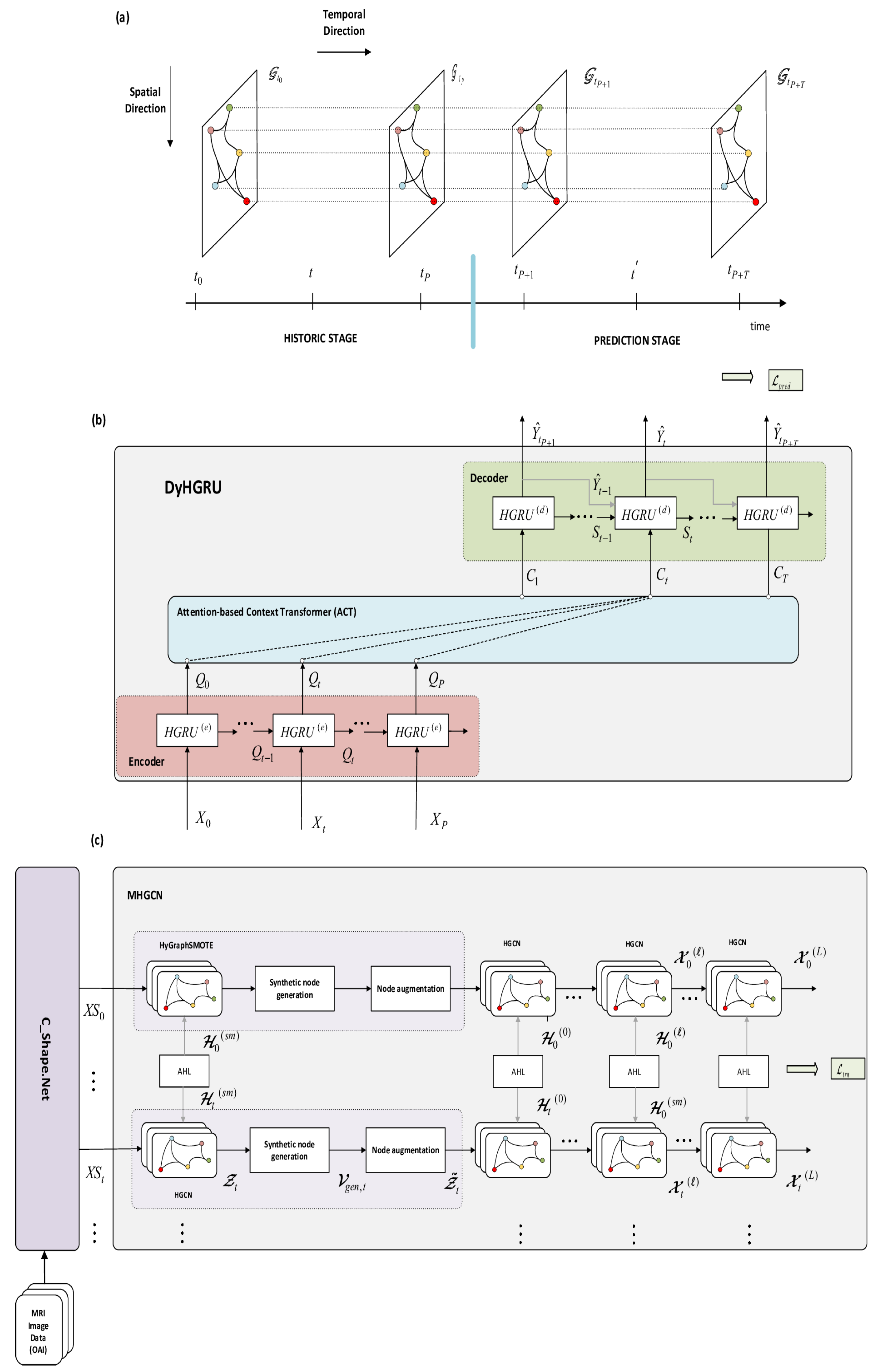
The general structure of the proposed DyHRM prediction network is depicted in Figure 2. The first part in this figure (Figure 2a) describes the spatio-temporal arrangement of knee data into a historical and prediction stage. The second part (Figure 2b) includes the crucial DyHGRU network undertaking the main prediction task. DyHGRU adopts an encoder–decoder architecture with hypergraph-gated GRU (HGRU) units. This model is designed to transform the knee sequences of hidden states in the encoder (historical stage) into label sequences of knees at the decoder (prediction stage). Finally, the third part (Figure 2c) illustrates the MHGCN network, which performs spatial HGCN convolutions at the different time steps of the historical stage. Also shown is the C_Shape.Net network, used to extract the 3D shape descriptors of knee cartilage from 3D MRI scans.

5.1. Data Representation and Notations

The knee record used in the following analysis includes the 3D shape descriptors obtained by the C_Shape.Net [25], the demographic features {age, BMI, gender}, and the historic sequence of knee injury. In our setting, the knee data are temporally distinguished into two stages, namely the historical stage and the prediction stage. The historical stage extends to a depth of P years, containing the the patient’s data at time steps { t 0 , t 1 , , t P } , where t 0 corresponds to the baseline visit. The prediction stage refers to the future period of the next T years { t P + 1 , , t P + T } .
Figure 2a shows the evolution of the different hypergraphs over time, indicating our spatial–temporal approach to how the patients’ knee data are represented. Along the vertical (spatial) direction, at each time slice t = t 0 , , , t P ; t P + 1 , , t P + T , knees are arranged to form a hypergraph, G t = V t , E t , H t , XS t . V t = v t ( i ) i = 1 N is the set of nodes ( | V t | = N ) , with each node v t ( i ) corresponding to a specific knee at time t. E t and H t represent the set of different hyperedges between the nodes and the incidence matrix, respectively, while XS t denotes the node data matrix of the hypergraph at time t. Moreover, along the horizontal (temporal) direction, each node is associated with a respective node sequence of shape data, evolving over time.
Given the maximum length of 8 follow-up years for the knee sequences, we consider historical data of varying depths, where P takes values in the range P { 0 , 1 , 2 , 3 } . The case of P = 0 corresponds to the graph data G 0 , which contains the population of N knees at the baseline visit. The case P = 1 subsumes the graphs { G 0 , G 1 } , including the 2 · N knees at the baseline and the first follow-up visit. Finally, the case P = 3 defines the maximum depth of the historical data, incorporating the 4 · N knees at the first four consecutive visits. Given a specific historical case { t 0 , , t P } , its respective prediction stage is extended to the next four successive time steps { t P + 1 , , t P + T } , i.e.,  T = 4 , where longitudinal KOA predictions are produced.
At the historical stage, the node data matrix XS t at time steps t = t 0 , , t P is defined as:
XS t = S ( v t ) / / I N J ( v t ) v t V t R ( N × ( F + 1 ) )
where S ( v t ) R ( F ) and I N J ( v t ) R denote the F-dimensional shape feature vector and the injury entry of node v t V t , respectively, at time t. The matrix XS P = ( XS 0 , , XS t , , XS P ) R P × N × ( F + 1 ) subsumes the node data at all time slices of the historical stage.
We also consider the label matrix Y t = y ( v t ) u t = 1 N R N × C , where y ( v t ) R C denotes the label vector of node v t at time t. The dimensionality of the label vector differs according to the prediction task being considered. Concretely, it takes the value C = 5 for node classifications into the five KL classes and  C = 2 for the binary progression problems. The matrix Y P subsumes the label vectors of nodes at all times of the historical stage: Y P = Y 0 , , Y t , , Y P R ( P × N × C ) . Similarly, we define the matrix Y T that incorporates the label vectors of nodes at the times t = t P + 1 , , t P + T of the prediction stage: Y T = Y t P + 1 , , Y t , , Y t P + T R ( T × N × C ) .
Viewing nodes (knees) temporally, we now consider the sequence of node v { 1 , N } :
NS ( v ) = v t 0 , , v t P ; v t P + 1 , v t P + T = NS P ( v ) ; NS T ( v )
where NS P ( v ) and NS T ( v ) denote the sequence parts corresponding to the historical and the prediction stage, respectively. The data sequence XS P ( v ) includes the node data (shape and injury) across all time steps of the historical stage:
XS P ( v ) = XS [ v t 0 , : ] , , XS [ v t , : ] , , XS [ v t P , : ] R ( P × ( F + 1 ) )
This sequence represents the shape evolution of a specific knee over historic times. We also consider the label sequences
Y P ( v ) = y ( v t 0 ) , , y ( v t ) , , y ( v t P ) R ( P × C )
and
Y T ( v ) = y ( v t P + 1 ) , , y ( v t ) , , y ( v t P + T ) R ( T × C )
for the historical and prediction stages, respectively.
In view of the above definitions, the general forecasting problem can be cast as a sequence-to-sequence learning task: Using the historical evolution of node data XS P , determine the multi-step ahead KOA predictions Y ^ T = Y ^ t P + 1 , , Y ^ t , , Y ^ t P + T R ( T × N × C ) . For each node, the above task implements a mapping between the sequences XS P ( v ) Y ^ T ( v ) for every v = 1 , , N . Notice that the shape descriptors and injury data are used solely at the historical stage, whereas they are disregarded in the prediction stage.

5.2. Imbalance of Knee Progressors

The DyHRM network is validated on different KOA incidence and progression tasks. In these problems, we seek to accurately detect the changes in KOA grades occurring over time, as the patient’s disease evolves from lower KL grades to more severe conditions.
Progression is measured here as the KOA grade change observed at a future target time t ( t P + 1 , t P + 2 , t P + 3 , t P + 4 ) with regard to a previous reference time t r e f = t P , i.e., the last time step of the historical stage, where the KOA labels are available. A knee is referred to as a progressor if it belongs to an inclusion set C i n c l at time t P , while simultaneously, its KOA evolution fulfills certain evaluation criteria at the target time t of the prediction stage. The node sequence attached to a knee progressor is then defined as a progressive node sequence. Depending on the progression task, C i n c l includes normal, doubtful, or moderate KOA grades. For instance, in KOA incidence, we consider C i n c l = { 0 , 1 } . On the other hand, the knee progress at t is evaluated using three different criteria: the change in KL grades ( Δ K L ) , the increase in JSN, or the decrease in JSW (Section 8.1).
Let P r o g r ( { k } ) and N o _ P r o g r ( { k } ) denote the set of progressor and non-progressor nodes of class k at reference time t P . The total number of progressors and non-progressors at this step is given by | P r o g r | = i = 0 4 | P r o g r ( { k } ) and | N o _ P r o g r | = k = 0 4 | N o _ P r o g r ( { k } ) | , respectively, where | · | denotes the cardinality of a set. These classes are highly imbalanced in the graphs. Concretely, Progr is a minority class containing considerably fewer knee progressors (10–15% of the total KOA patients), compared to No_Progr, which is the majority class. The imbalance ratio IR = | P r o g r | | N o _ P r o g r | 1 is used to measure the extent of class imbalance. The relative scarcity of progressors is a serious concern in KOA analysis that hinders their accurate detection, thus leading to suboptimal classifications. To cope with the above issue, we apply here the proposed HyGraphSMOTE approach to obtain balanced knee datasets, adapted to each experimental case individually (Section 6.2).

6. Multi-View Hypergraph Convolutional Network

Before entering the DyHGRU network, the node data are preprocessed by the MHGCN module, which conducts P independent convolutional branches (Figure 2c). Each branch involves two parts, namely the HyGraphSMOTE module used to balance the knee datasets and the multi-view HGCN convolutions on the hypergraphs G t , t = 1 , , P of the historical stage. The aim of this task is to acquire more comprehensive node representations, taking into consideration various relationships among the nodes.

6.1. Adaptive Hypergraph Generation

For the formation of the hyperedges, we consider four different views, corresponding to the shape features and the three demographic features, respectively:
H t = H t ( s p ) , H t ( A g e ) , H t ( B M I ) , H t ( G e n d e r ) R ( N × M )
H t ( s p ) includesthe spectral affinities between the nodes, i.e., the similarities between their global shape features. These hyperedges are adaptively constructed using the AHL mechanism in Section 3.2. The latter three hyperedges in Equation (10) encode the pairwise node relations in terms of age, BMI, and gender and are determined differently. Specifically, the age domain is distinguished into four age groups (hyperedges): { < 50 , ( 50 , 59 ) , ( 60 , 69 ) , 70 } . Each hyperedge is described by a membership function μ j ( x ) = exp ( x p j ) 2 σ 2 , j = 1 , , 4 , where p j is the central value of the group and σ is the standard deviation between all nodes in V t . Then, the degree of membership of the i-th node in the j-th hyperedge is defined as H t ( A g e ) ( i , j ) = μ j ( x i ) [ 0 , 1 ] . Similarly, we create four hyperedges for H t ( B M I ) and two hyperedges for H t ( G e n d e r ) , respectively, leading to a total number of M = N + 10 hyperedges. Contrary to the spectral H t ( s p ) , which is adaptively computed across the different layers and time steps, the three demographic incidence matrices remain fixed.

6.2. HyGraphSMOTE Balancing Method

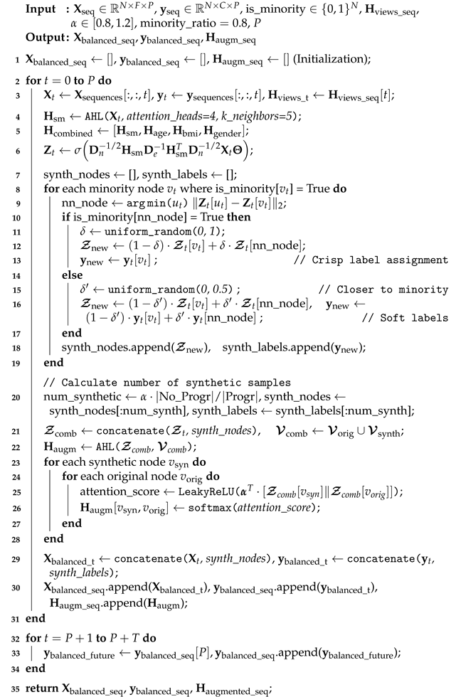
The aim of this process is to balance the classes of progressors (minority) and non-progressors (majority) on the hypergraphs G t , t = t 0 , , t P . This is achieved through minority oversampling, i.e., generation of synthetic nodes of the minority class of progressors. The new examples are generated by interpolating between a target minority node and its nearest neighbor. The HyGraphSMOTE method comprises three stages: embedding of the input data, synthetic node generation of the progressor class, and hyperedge generation. The following paragraphs contain a detailed breakdown of the overall process. Algorithm A1 in Appendix A provides a comprehensive step-by-step guide for all stages of the procedure.
  • Data Embedding: In this stage, the input data XS t are transformed into an embedding feature space Z t R ( N × F ( s m ) ) . Instead of applying minority oversampling over the original raw data, the new space provides more discriminating node representations, especially for the progressor ones. Since HyGraphSMOTE is designed on the hypergraph framework, the embedded features are acquired via a HGCN convolution:
    Z t = σ G H XS t , H t ( s m ) ; W t ( s m ) , Θ t ( s m )
    Z t = Z t [ v t ] v t V t , where Z t [ v t ] denotes the embedding of node v t at time t. Furthermore, W t ( s m ) and Θ t ( s m ) contain the learnable hyperedge weights and the filter parameters, respectively. H t ( s m ) denotes the incidence matrix at the SMOTE phase, as described in Equation (10). This matrix plays the role of a hyperedge generator, incorporating the multiple view hyperedge connections between the nodes. Here, H t ( s m ) is adaptively learned from node features using the attention-based AHL mechanism in Section 3.2: H t ( s m ) = A H L ( XS t , V t ) .
  • Synthetic Node Generation: Let v t be a minority node at time t with an embedding feature Z t [ v t ] . The first step is to find its nearest neighbor node in the embedding space, defined as follows:
    n n ( u t ) = a r g m i n u t Z t [ u t ] Z t [ v t ] 2
    Minority oversampling generates two types of synthetic nodes by interpolating between the pairs ( v t , n n ( v t ) ) . In the first main case, we consider that n n ( v t ) is also a minority node. The new node v ¯ t is created as follows:
    Z [ v t ¯ ] = ( 1 δ ) · Z [ v t ] + δ · Z ( n n ( v t ) ) , s . t . y ( v t ¯ ) = y ( v t )
    where δ is a uniformly distributed random variable in the range [ 0 , 1 ] . Since both v t and n n ( v t ) are close neighbors of the minority class, node v ¯ t is crisply assigned to the same class. In the second case, the synthetic nodes are generated from mixed node pairs ( v t , u t ) , considering that the nearest neighbor u t = n n ( v t ) now belongs to the majority class. In that case, interpolation is applied on both the embedding and the label space, simultaneously. The feature and the label of the new mixed nodes are determined as follows:
    Z [ v ^ t ] = ( 1 δ ) · Z [ v t ] + δ · Z [ u t ]
    y ( v ^ t ) = ( 1 δ ) · y ( v t ) + δ · y ( u t ) , y ( u t ) y ( v t )
    where Z [ v ^ t ] , y ( u ^ t ) are the embedding and the label of the newly generated mixed node v t ^ . Contrary to the previous case, the mixed nodes receive soft (fuzzy) label vectors, taking values between the minority and the majority ones. δ is a random variable in the range [ 0 , b ] , where b is set to a value of 0.5 in the experiments. This choice of b suggests that both the embedding and the label of node v ^ t are placed by Equations (14) and (15) closer to the minority node v t rather than its nearest neighbor majority node u t . The incorporation of the mixed nodes tends to make the boundaries between classes smoother, thus facilitating better performance in the classification task. In the experiments, we apply a proportion of 80 20 % of synthetic nodes, focusing primarily in generating new nodes from strictly minority node pairs and a smaller percentage from mixed pairs. The synthetic node generation on a minority class is carried out according to an oversampling rate O v r r a t e = α · | N o _ P r o g r | / | P r o g r | , where the parameter α { 0.8 , 1.2 } controls the balance between the minority (progressor) and the majority (non-progressor) classes.
    The next step is to formulate the balanced graph G ˜ t = V ˜ t , E ˜ t , H ˜ t ( s m ) , Z ˜ t at each time t via data augmentation. V ˜ t = V t V g e n , t augments the existing node set with the set of synthetic nodes V g e n , t = { v ¯ t , v ^ t } . The augmented V ˜ t contains a total of N ˜ = N + | V g e n , t | nodes. Similarly, Z ˜ = Z t Z g e n , t concatenates the embeddings of the respective node sets. Finally, H ˜ t ( s m ) represents the hyperedge connections between existing nodes, as well as pairwise links between the synthetic nodes and the existing ones. This matrix is adaptively constructed again as H ˜ t ( s m ) = A H L ( Z ˜ t , V ˜ t )
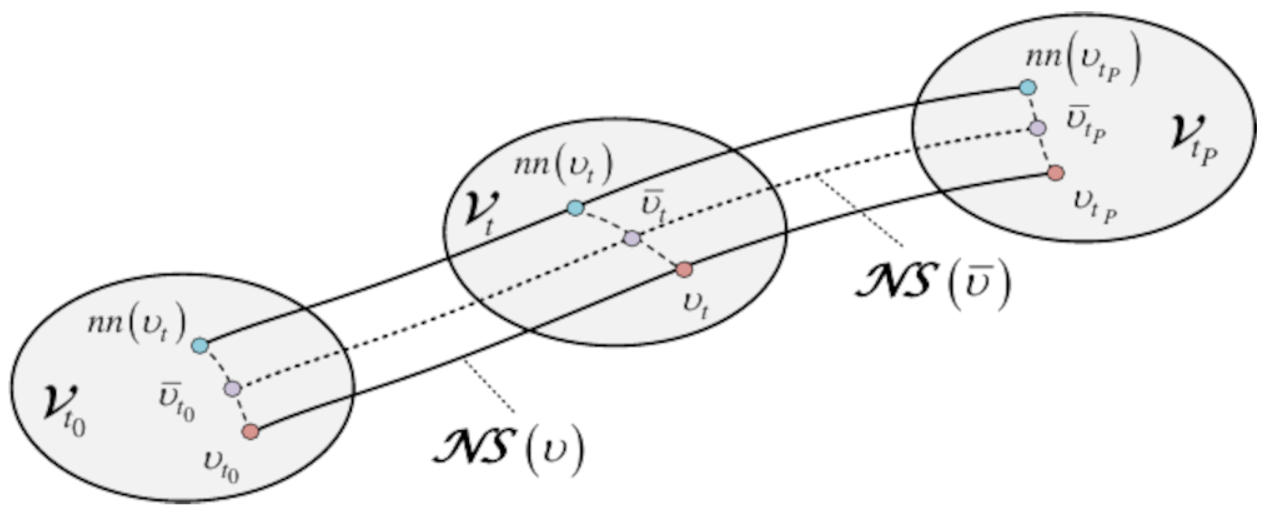
  • Generation of Synthetic Sequences: The last stage of data balancing is to synthesize new progressive node sequences NS ( v ˜ ) = { NS P ( v ˜ ) ; NS T ( v ˜ ) } by repeatedly applying node oversampling over the different time steps. The sequence oversampling is visualized in Figure 3 and proceeds along the following steps:
    (a)
    At the historic stage, define the set of progressor nodes of the original dataset at the terminal step t P and restore their respective node sequences NS P ( v ) . The terminal nodes are distributed over the different KL classes of an inclusion set C i n c l .
    (b)
    For each t = t 0 , , t P , find the nearest neighbor nodes n n ( v t ) from Equation (12). As an outcome, we obtain the nearest neighbor sequence of NS P ( v ) .
    (c)
    Generate a synthetic node sequence NS P ( v ˜ ) = { v ˜ t 0 , , v ˜ t P } using either Equation (12) or Equations (14) and (15) to compute the features and labels of the pertaining nodes. Temporally, the new sequence evolves in the vicinity of NS P ( v ) ; hence, the corresponding nodes receive the same or similar labels as in the original sequence.
    (d)
    At the prediction stage, we assume that the label sequence Y T ( v ˜ ) follows a similar track as Y T ( v ) ; thus, we set y ( v ˜ t ) = y ( v t ) for t = t P + 1 , , t P + T .

6.3. HGCN Convolutions

The node representations Z ˜ t R ( N ˜ × F ( s m ) ) obtained after HyGraphSMOTE are subject to spatial HGCN convolutions in MHGCN at each time step of the historical stage. Convolutions are applied on the balanced graphs G ˜ t , t = t 0 , , t P . The future embeddings X t ( l ) R ( N ˜ × F ( l ) ) acquired at layer l = 0 , 1 , , ( L 1 ) are given as follows:
X t ( l + 1 ) = σ G H U t ( l ) , H t ( l ) ; W t ( l ) , Θ t ( l )
where W t ( l ) R ( N ˜ × F ( l ) ) and Θ t ( l ) R ( F ( l ) × F ( l + 1 ) ) are the tuneable matrices containing the hyperedge weights and the filter parameters, respectively. U t ( l ) is the input data at layer l, taken as U t ( 0 ) = Z ˜ t for the first layer and U t ( l ) = X t ( l ) for the subsequent layers. Finally, H t ( l ) denotes the incidence matrix including the multi-view hyperedge connections among the nodes. For  l = 0 it is defined as H t ( 0 ) = H ˜ t ( s m ) , while for later layers, it is dynamically constructed by H t ( l ) = A H L ( X t ( l ) , V t ) . To facilitate the signal flow and enhance the learning efficiency, we use residual connections between the convolutional units. Further, as shown in Figure 2c, the attention mechanism used in both HyGraphSMOTE and the HGCN convolutions for the derivation of H t ( s m ) and H t ( l ) is shared across the different times of the historical stage. The outputs of the MHGCN network serve as inputs to the encoder at each time t, i.e., X t = X t ( L ) , t = t 0 , , t P .

7. Dynamic Hypergraph Gated Recurrent Unit

The main DyHGRU network has an encoder–decoder architecture, aiming to generate multi-step-ahead predictions of progression for the KOA tasks. The encoder contains the hypergraph-gated recurrent units, HGRU(e), while the decoder contains the respective HGRU(d) units. We also have the attention-based context transformer (ACT) to coordinate between the encoder and decoder. In the following, we detail every constituent part of the DyHGRU network.
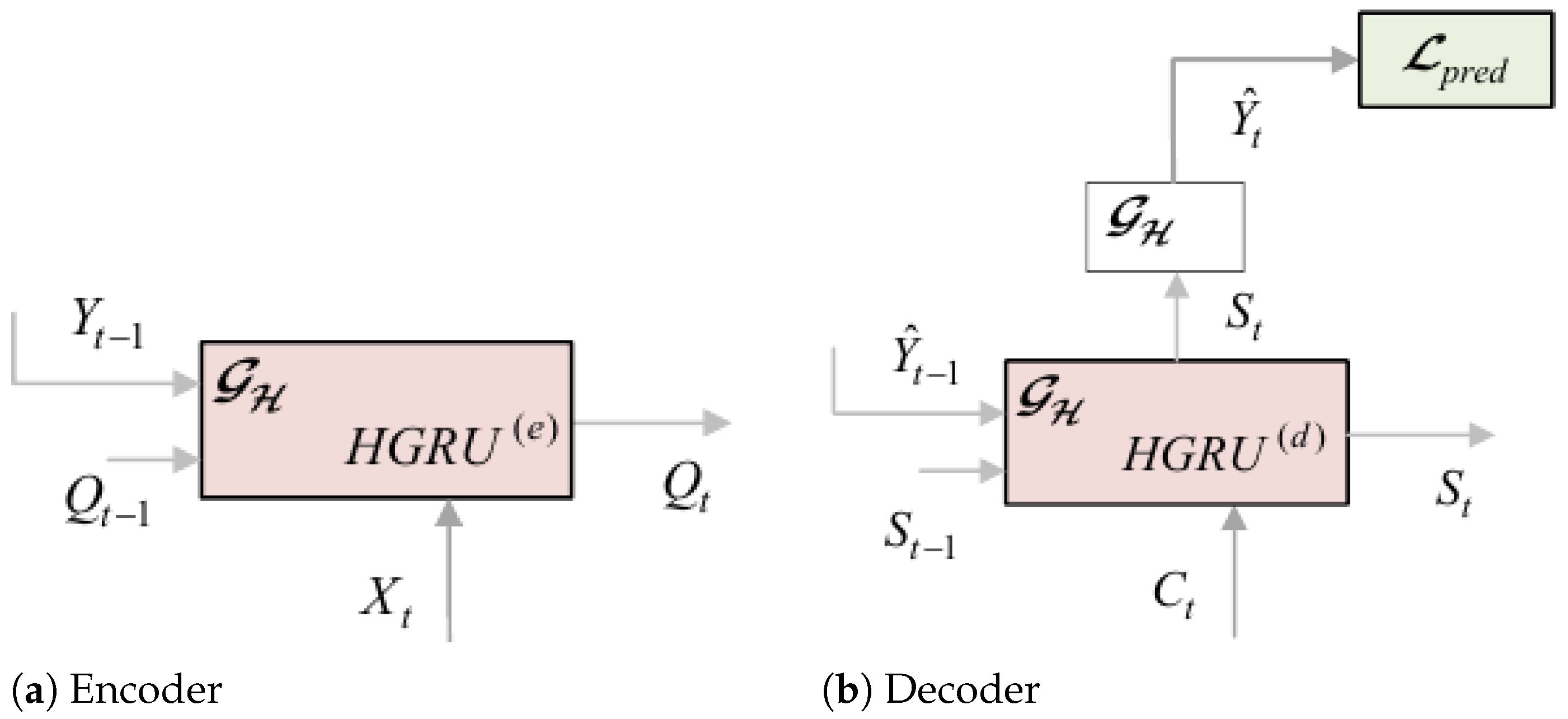
  • Encoder: The encoder receives a sequence of knee data { X 0 , , X t , , X P } to generate a sequence Q 0 , , Q t , , Q P of hidden states. The HGRU(e) model at time t is outlined in Figure 4a and is functionally described by Q t = F Q ( e ) X t , Q t 1 , Y t 1 ; Θ Q ( e ) , where X t R ( N ˜ × F ( L ) ) , Q t R ( N ˜ × d ) and Y t R ( N ˜ × C ) are the external input, the d-dimensional hidden state of HGRU(e), and the ground true labels of nodes. We use the GRU as a building module, a variant of recurrent neural networks, which is suitable for effectively handling time-series data. Moreover, inspired by [59], we integrate the temporal capabilities of GRUs with the spatial HGCN convolutions to create the proposed HGRU(e) module with spatio-temporal processing capacities. This is achieved by replacing the linear transformations in GRUs with hypergraph aggregations. The computations involved in HGRU(e) are described as follows:
    R t ( e ) = σ G H X t , Q t 1 , W Y Q ( e ) · Y t 1 , H ( e ) ; W ( e ) , Θ R ( e ) + b R ( e )
    U t ( e ) = σ G H X t , Q t 1 , W Y Q ( e ) · Y t 1 , H ( e ) ; W ( e ) , Θ U ( e ) + b U ( e )
    Q ˜ t = σ G H X t , W Y Q ( e ) · Y t 1 , R t ( e ) Q t 1 , H ( e ) ; W ( e ) , Θ Q ˜ ( e )
    Q t = U t Q t 1 + 1 U t ( e ) Q ˜ t
    The operator [ · , · ] denotes concatenation of the input entries, and ⊙ represents the Hadamard product operator. R t ( e ) and U t ( e ) are the reset gate used to discard redundant previous information and the update gate that controls the output. The set of tunable parameters includes the following: H ( e ) and W ( e ) are the incidence matrix and the hyperedge weights involved in the HGCN convolutions in HGRU(e), while W Y Q ( e ) is an embedding matrix used for dimensionality matching of the labels Y t 1 . Furthermore, the sets Θ R ( e ) , b R ( e ) , Θ U ( e ) , b U ( e ) and Θ Y ( e ) , b Y ( e ) are the filter parameters and bias terms pertaining to the R t ( e ) , U t ( e ) , Q ˜ t , and  Y ^ t , respectively. The set of learnable parameters discussed above are shared across all HGRU(e) units of the encoder for t = t 0 , , t P .
  • Decoder: The decoder shares a similar structure as the encoder, comprising a total of THGRU(d) units (Figure 4b) for t = t P + 1 , , t P + T . It takes as input the context sequence { C 1 , , C t , , C T } and produces the sequence of label estimates Y ^ T = Y ^ t P + 1 , , Y ^ t , , Y ^ t P + T at the prediction stage. Functionally, the decoder units are described by S t = F S ( d ) C t , S t 1 , Y ^ t 1 ; Θ S ( d ) and Y ^ t = F Y ( d ) S t ; Θ Y ( d ) , where C t , S R ( N ˜ × d ) are the context input and the output of the HGRU(d), and  Y ^ t R ( N ˜ × C ) denotes the label estimates of nodes at time t. The respective convolutions of the HGRU(d) units are given as follows:
    R t ( d ) = σ G H C t , S t 1 , W Y S ( d ) · Y ^ t 1 , H ( d ) ; W ( d ) , Θ R ( d ) + b R ( d )
    U t ( d ) = σ G H C t , S t 1 , W Y S ( d ) · Y ^ t 1 , H ( d ) ; W ( d ) , Θ U ( d ) + b U ( d )
    S ˜ t = σ G H X t , W Y S ( d ) · Y ^ t 1 , R t ( d ) S t 1 , H ( d ) ; W ( d ) , Θ S ˜ ( d ) + b S ˜ ( d )
    S t = U t ( d ) S t 1 + 1 U t ( d ) S ˜ t
    Y ^ t = σ G H S t , H ( d ) ; W ( d ) , Θ Y ( d ) + b Y ( d )
    where S ˜ t R ( N ˜ × d ) are the candidate hidden activations, and  R t ( d ) , U t ( d ) are the reset gate and update gate, respectively. The first four equations (Equations (21)–(24) represent the internal convolution dynamics of the HGRU(d), while the last equation Equation (25)) is a convolution aiming to yield the label estimates Y ^ t of nodes from hidden states of the decoder at follow-up time t. The terminology and the usage of the various parameters in the decoder are similar to the ones in the encoder part.
  • Attention-Based Context Transformer: The ACT module acts as an interface between the encoder and the decoder parts. Concretely, it transforms the sequence of hidden states Q 1 , , Q t , , Q P acquired by the encoder into a sequence of context input vectors C 1 , , C t , , C T for the decoder. The context vectors C t at future times are determined by selectively applying multi-head attention to relevant time steps of the hidden sequence Q 1 , , Q t j , , Q P . Let γ t , t j ( k ) ( v ) denote the attention score between the weights C t and Q t j , t j = t 1 , , t P for a node v = 1 , , N ˜ . The superscript ( k ) indicates the k-th attention head, k = 1 , , K . The attention scores are adaptively derived as follows:
    λ t , t j ( k ) ( v ) = R e L U α T · S t 1 [ v ] · Θ t r , S ( k ) Q t j [ v ] · Θ t r , Q ( k ) γ t , t j ( k ) = exp λ t , t j ( k ) ( v ) t r = t 0 t P 1 exp λ t , t r ( k ) ( v )
    where the index [ v ] indicates the v-th row of the respective matrices. The context value C t is obtained as a weighted sum from all historical time steps over the different attention heads:
    C t [ v ] = k = 1 K t j = t 0 t P 1 γ t , t j ( k ) Q t j [ v ]
    The calculations in Equations (26) and (27) are conducted in parallel, and the learnable parameters are shared across all nodes and time steps. According to Equation (27), the context vectors aim to identify the informative trends of the encoder evolution. Particularly, they seek to detect aggravation of JSN, which is a valuable indication to assess KOA progression. In that respect, the context sequence allows the decoder to acquire the correct track of S t P + 1 , , S t , , S t P + T and Y ^ T until the target follow-up time t is reached, where the progression level should be eventually evaluated.
  • Network Training: Training is performed here following the semi-supervised learning (SSL) framework. In this setting, the input data XS P comprises a labeled part XS P , l R ( N l × P × D ) of N l nodes and an unlabeled part XS P , u R ( N u × P × D ) of N u nodes, with  N = N l + N u . The former part contains nodes with historical shape sequences having labeled sequences of KOA grades in the prediction stage. The nodes in the latter part form the testing dataset; hence, their output label sequences are unknown. Under SSL, we exploit the shape content of both the training and testing data, which can yield better results.
    Learning of the DyHRM predictor is carried out in two phases. In phase 1, we conduct a node classification task to pretrain the branches of the MHGCN network at the historical time steps. The cross-entropy loss is used to match the estimates Y ^ P to the true labels Y P in the KL classes ( C = 5 ) :
    L t r n Y ^ P , Y P = t = t 0 t P c = 1 C Y P ( t , c ) · ln Y ^ P ( t , c )
    Pretraining aims to initialize the features of the real labeled and unlabeled nodes, and especially the synthetically ones generated by HyGraphSMOTE. Next, phase 2 performs end-to-end training of the entire network in Figure 2, including the DyHGRU, MHGCNs, and the C_Shape.net. The goal is mainly to optimize the future estimates Y ^ T given by the decoder using a regularized objective described as follows:
    L = λ t r n L t r n Y ^ P , Y P + λ p r e d L p r e d Y ^ T , Y T
    where L p r e d is a loss function defined on the progression classes ( C = 2 ) :
    L p r e d = t = t P + 1 t P + T c = 1 C Y T ( t , c ) · ln Y ^ ( t , c )

8. Experimental Results

In this section, we evaluate the performance of the proposed DyHRM predictor on the KOA incidence and progression tasks using the OAI cohort. In the experiments, we assess the quality of the produced longitudinal predictions for varying depths of the historical stage ( P ) . We also elaborate on the generation of balanced datasets and conduct several ablation studies to examine the effects of various parts in our approach.

8.1. Configuration of Progression Tasks

Table 1 hosts the inclusion set and the evaluation criteria used for the definition of the five progression tasks examined in the experiments. KOA incidence (onset) is usually defined as knees with N o _ K O A ( C i n c l = { 0 , 1 } , K L 1 ) at the reference time step t P , which are then progressing to higher KL grades { 2 , 3 , 4 } , i.e., doubtful, moderate, or severe KOA. The presence of incidence is assessed at t P + 4 using two evaluation criteria, namely the change in KL grade ( K L 2 ) and the increase in joint space narrowing score ( Δ J S N 1 ) . KOA progression is defined as knees with visible KOA at t P ( C i n c l = { 2 , 3 } , 1 < K L < 4 ) and higher KL scores at follow-up times. Progression is commonly evaluated in the literature using three criteria: the change in KL grades ( Δ K L 1 ) , the increase in medial joint space narrowing ( Δ m J S N 0.5 ) , or the decrease in joint space width ( Δ J S W 0.7 ) . [24]

8.2. Dataset Generation

For each historic depth, we hereby create individual balanced datasets for training under specific progression scenarios according to their respective inclusion set and evaluation criterion. Dataset formation follows a two-stage procedure. At stage-1, we generate an initial imbalanced dataset considering the population of knees with complete record data across the entire range of follow-up years. Initially, from the collection of knees v t C i n c l at the reference time step t = t P , we identify the subset of knee progressors after evaluation at the final step t P + T . Next, we restore the progressing knee sequences NS ( v ) = NS P ( v ) ; NS T ( v ) , v P r o g r , comprising the evolving parts during the historic and the prediction stage, respectively. The above set of progressors is supplemented with an amount of non-progressive knee sequences passing through the KL classes of C i n c l . We retain an approximate proportion of 15–85% between progressors and non-progressors, leading to an initial imbalanced dataset with IR 0.18 . The last step applies the proposed HyGraphSMOTE algorithm to balance the initial dataset by synthesizing new progressing knee sequences (Section 6.2).
Table 2 exemplifies the dataset construction of a KOA progression scenario using a historic depth of P = 2 . In that case, we have an inclusion set C i n c l = { 2 , 3 } , while the presence of progression is assessed at t = t 6 using the Δ K L 1 criterion. This table presents the distribution of KL grades for the non-progressors, the progressors, and the synthetically generated knees. We show the knees pertaining to the KL classes at reference time t = t 2 , as well as the knee distribution at the historic time steps t 0 , t 1 . The balancing of progressing knee sequences is performed via oversampling on the minority class with O v r r a t e = 78 % . Synthetic nodes are created from strictly minority or mixed node pairs to a ratio of 75–25%. The total number of knees N ˜ (last row) represents the cardinality of the augmented node sets at the historic time steps: | V ˜ t 0 | = | V ˜ t 1 | = | V ˜ t 2 | = N ˜ . The datasets attached to the other progression cases are created in a similar way. The suggested construction of balanced datasets achieves two goals: (a) sufficient node data for learning of complex deep networks to avoid overfitting, and (b) balanced representation of knee progressors class, leading to more robust classification of KOA progression.
Knee data were randomly partitioned into three non-overlapping datasets for training, validation, and hold-out testing with a proportion of 60–20% and 20 % , respectively. For the training and validation datasets, we retained a balanced representation between the knee progressors (real and synthetically generated) and the non-progressors. The HyGraphSMOTE balancing algorithm for generating synthetic nodes and sequences was applied independently on each fold to control for any data leakage issues and to facilitate the robustness of the reported performance metric. However, it should be stressed that for the hold-out testing dataset, we exclusively considered the real knee progressors.
The progression tasks are cast as binary classification problems at the different time steps of the prediction stage ( C = 2 ) . Classification performance is measured using the Area Under the Curve (AUC) values. The various hyperparameters pertaining to our predictor network are selected via 5-fold cross-validation. Finally, the reported accuracies are obtained by averaging the results over the five different data folds.

8.3. Implementation Details

The models presented in this study were primarily developed within the PyTorch 2.7.1 deep learning framework (https://pytorch.org/). The original surface and volumetric features used to generate the initial set of input features in the C_Shape.Net were extracted via the use of the Trimesh (https://trimesh.org/ (accessed on 1 June 2025)) library. In order to streamline and monitor the hyperparameter optimization procedure, we made use of the Optuna (https://optuna.org/ (accessed on 1 June 2025)) open-source optimization framework and performed an extensive hyperparameter search utilizing the Bayesian hyperparameter optimization process [73]. The model was trained for a maximum number of 1000 epochs, with an early stopping criterion halting the training process once the validation loss failed to improve for 20 consecutive epochs. The initial learning rate was set to 0.1, with the inclusion of a multi-step learning rate scheduler that decays that number by a factor of 10 at 3 evenly spaced milestones (250, 500, and 750 epochs, respectively). The source code containing the implementation of the various modules of the proposed DyHRM, feature extraction, and subsequent balancing, as well as the design of the overall training and validation processes, can be found at https://gitlab.com/koa_prediction/spthgnn_encoder_decoder (accessed on 18 August 2025). Pre-trained weights for the case of P = 4 are also available in the repository for each component of the overall architecture. Table 3 hosts a summary of the hyperparameters tested, their ranges, and their corresponding ultimate optimal values.

8.4. Longitudinal Predictions of KOA Incidence

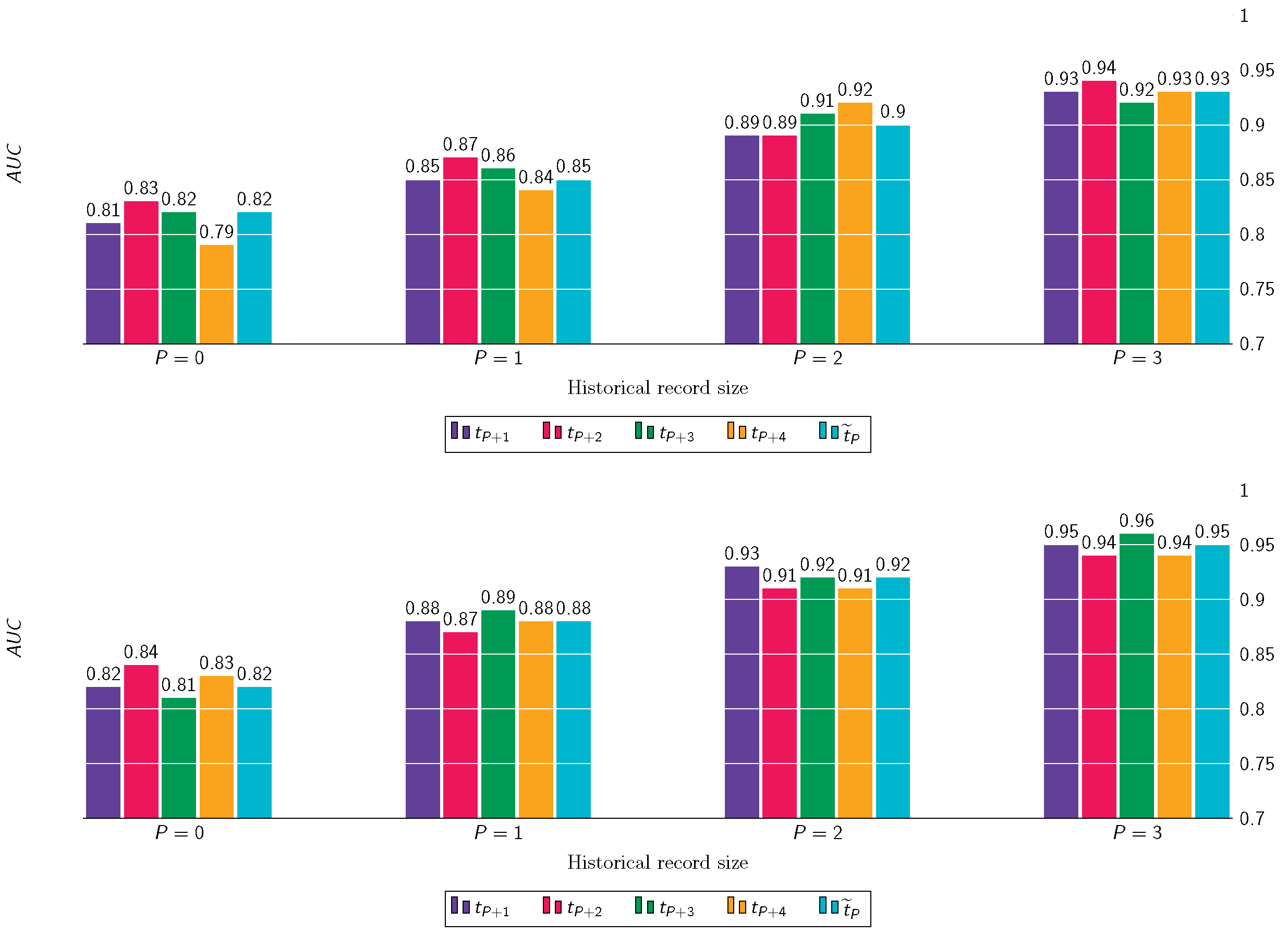
Figure 5 presents the longitudinal predictions of the KOA incidence task for varying depths of the historical stage, defined by the evaluation criteria K L 2 and J S N 1 . Accuracies are evaluated in terms of the A U C values at { t P + 1 , t P + 2 , t P + 3 , t P + 4 } and the A U C of average predictions over the follow-up period. In these barplots, we examine short-term predictions at { t P + 1 , t P + 2 } and medium-term predictions at { t P + 3 , t P + 4 } . In incidence, the knee (node) sequences of cartilage shapes/volumes remain at KL grades of { 0 , 1 } (no KOA indication), and the predictor aims to identify subsequent progress to higher KL conditions.
Figure 5 shows similar performance for both definitions of incidence, with a slight superiority for the J S N 1 criterion. Focusing on this latter case, the following observations can be drawn. First, the historic depth has a significant impact on the obtained prediction performance. Specifically, the larger the size of the historic node sequences, the higher the accuracies produced at follow-up times. The worst performance is obtained for P = 0 , which provides an average A U C = 0.82 . In that case, learning is confined solely to the baseline data, while the encoder is condensed to a single unit at t = t 0 . Increasing the depth of historic sequences presented to the encoder manages three goals simultaneously: (a) it enables the encoder to generate a comprehensive hidden sequence Q t = t 0 t P representative of cartilage volume variations, (b) it allows the ACT module to identify discriminating trends of KOA development across the historic evolution, and (c) it allows the decoder to acquire a more accurate sequence Y ^ t = t P + 1 t P + T of progression assessments at the prediction stage. The best results are obtained for the maximum historic depth of P = 3 , which provides a considerably higher average A U C = 0.95 . The second observation is that the multi-step predictions retain similar accuracies across the different follow-up times. This underscores the capability of DyHRM to produce consistent predictions ahead, to an accuracy level dictated by the historic depth ( P ) . The above observations apply similarly to all experiments presented in the sequel.
In the following, the incidence task is decomposed into two distinct sub-tasks. In the first sub-task, we consider the early KOA detection problem, whereby a knee advances from non to doubtful KOA ( K L : { 0 , 1 } 2 ) . The second sub-task examines the case where a knee advances from non to moderate or severe KOA. Figure 6 shows the prediction performance on these two sub-tasks for the two definition criteria and for varying historic depths P. Accuracies are measured in terms of A U C values of average predictions over the prediction horizon. As can be seen, the criterion J S N 1 provides slightly better accuracies compared to K L 2 . For the more challenging early detection task, the predictor provides increasing accuracies in the range [0.83, 0.85, 0.89, 0.92], as the depth varies for P = 0 to P = 3 . For the second sub-task, we obtain accuracies of [0.84, 0.87, 0.91, 0.95] for increasing P values. This sub-task handles a relatively relaxed classification problem with more discriminating classes, which justifies the improved performances. The precise predictions of KOA incidence acquired over short-term and middle-term time steps ahead is valuable for patients with minimal symptoms, since it can assist clinicians in scheduling effective treatment strategies.
Table 4 presents comparative results of our approach with existing works in the literature on the incidence task. We included methods with a similar inclusion set, different evaluation criteria of incidence, and radiographic biomarkers, used as inputs to the respective risk models. For fair comparisons, most of the methods make use of the OAI dataset. All these approaches consider the knee data at baseline ( P = 0 ) and predict KOA incidence at a single target follow-up time, usually 48 months ahead. As can be seen, the  A U C values obtained by our predictor for P = 0 are comparable or better than the ones of the competing methods. However, for longer historic depths, we were able to acquire considerably better accuracies at multiple steps ahead, which underlines the important role of incorporating past sequence data in incidence predictions.

8.5. Longitudinal Predictions of KOA Progression

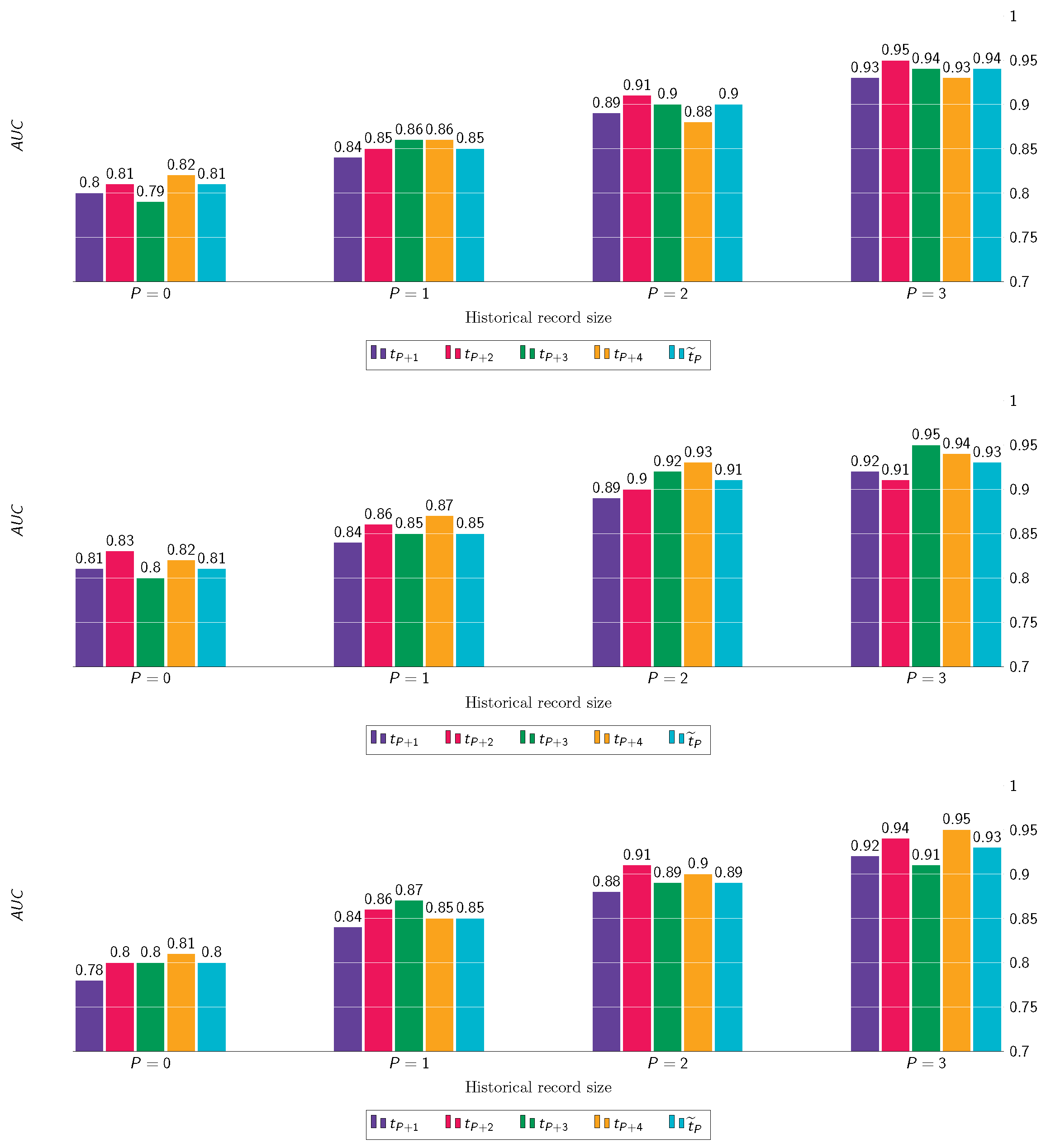
Figure 7 shows the longitudinal predictions for the KOA progression task for varying depths of the historical stage. We present results corresponding to three definition criteria of progression in Table 1, i.e., Δ K L 1 ,   Δ m J S N . 5 , and Δ J S W 0.7 . In KOA progression, there is sufficient variation in past knee sequences over time. Concretely, they proceed from lower KL scores { 0 , 1 } during the historic stage, passing finally through the inclusion set { 2 , 3 } of minimal or moderate KL grades at t P . The goal of the predictor is then to assess the progress to moderate or severe KL grades at follow-up times.
The results show a similar progression performance for the three definition criteria across the different historic depths and follow-up times. In terms of the Δ K L 1 criterion, our approach achieved sufficiently high average values of A U C : [ 0.81 , 0.85 , 0.90 , 0.94 ] for increasing historic depths. The lowest results were obtained using only the baseline visit data. For larger historic depths, we achieved considerably better accuracies, indicating again the impact of historic data on the predictions of progression. In this task, DyHGRU was allowed to detect the temporal dynamics from historical knee sequences and effectively transform those sequences into future progression assessments.
Table 5 compares our approach with other methods in the literature on the progression task. We included related methods with similar inclusion sets and different definition criteria of progression, using mostly the OAI repository. Most of these methods make use of the baseline data, i.e., they disregard historical data of knees and predict KOA progression at a specific target time ahead. The works in [16,17] produce longitudinal predictions in a static manner by creating distinct mappings from the baseline visit to each follow-up time. As can be seen, our A U C values obtained for P = 0 (baseline) are favorably comparable to the ones of the existing methods. However, for greater depths, our approach produced higher accuracies on the progression task across all the different definition criteria.

8.6. Long-Term Predictions of KOA Incidence and Progression

Next, we examine the efficiency of DyHRM to provide long-term KOA predictions, i.e., predictions at a larger future horizon 4 < T 7 . Figure 8 shows the average A U C values at the follow-up times t 5 ,   t 6 , and t 7 , with respect to the baseline visit for the KOA incidence and progression and for varying historic depths. The results show that, for both tasks, the historic depths of P = 1 and P = 2 yield considerably better accuracies compared to P = 0 . At the terminal time step t 7 , DyHRM yields A U C values in the range [0.77, 0.84, 0.88] and [0.78, 0.84, 0.91] for the incidence and progression, respectively, and for increasing depths P = 0 , 1 , 2 .

8.7. Demographic-Based Accuracies

Table 6 shows the prediction performance for the KOA incidence and progression tasks, corresponding to the different demographic groups categorized by age, BMI, and gender. Accuracies are measured based on the average A U C values over all times ahead for the different historic depths. For the incidence problem, we observe similar performance for the different groups, with a slight superiority of the elderly group, as well as the pre-obese and obese groups, over the respective groups of age and BMI categories. In the progression problem, however, there are more clear distinctions among the different groups. Concretely, the male group exhibits consistently higher accuracies compared to the female group. For the age groups, we can notice a trend of increasing performance as age advances from younger to mode elderly patients. For the BMI groups, we also observe a clear trend of increasing accuracies as BMI moves from the normal to the obese cluster. In both incidence and progression, predictions are improved for larger historic depths, while the differences and trends become more distinct, especially for the progression task. This is attributed to the fact that the larger amount of information conveyed by longer knee sequences allows the predictor to yield more precise KOA assessments.

8.8. Test Case Demonstration

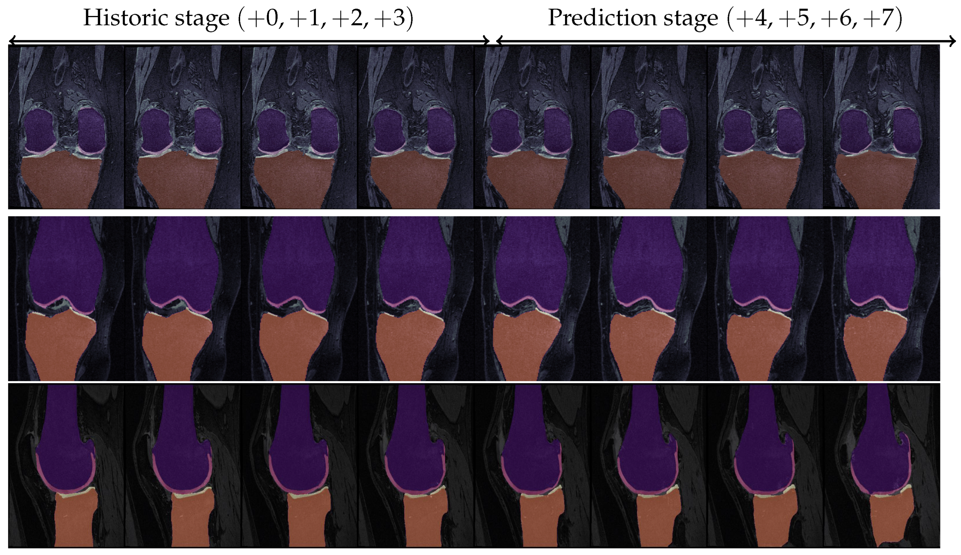
This section illustrates a visual demonstration of the KOA progression predictions for two specific knees at all historical and future time points. Figure 9 showcases the gradual cartilage degradation in the coronal plane. Table 7 provides a summary of the longitudinal progression predictions in contrast to the actual progression incidence values for all the time steps corresponding to the future stage.

8.9. Ablation Studies

The experiments in this section aim to demonstrate the impact of the different parts pertaining to our DyHRM predictor. Table 8 hosts the results for the KOA incidence problem and for various historic depths. The full scheme refers to the complete model configuration, including the seven factors cited in the following. The contribution of each factor is measured as the performance reduction in AUC, which is obtained after disregarding this factor from the full scheme. As can be seen, the oversampling of progressive knee sequences via HyGraphSMOTE has a significant effect on the performance, varying in the range [4.96–6.02%] across the various depths. This finding advocates the usage of dataset balancing for learning of large risk models, especially for small datasets and/or with a limited number of knee progressors for a given task. To measure the effect of demographic factors, we remove the corresponding hyperedge incidence matrices (views) from HGCN convolutions (Section 3.2). These factors have a noticeable contribution of [2.81–3.12%] across P, while the injury history has a relatively smaller impact of [1.61–2.18%]. Further breaking down the various types of demographic hyperedges, we measure the effect of discarding a single such variable each time (Age, BMI, Gender) and recoding the influence on the resulting performance of the overall model. The reported results suggest that among these variables, the strongest influence is exerted by the Age and BMI groups, with Gender holding slightly diminished relevance.
The SSL approach has an important effect on the performance, ranging between (5.17 and 7.02%). This indicates that the combined usage of both labeled and unlabeled node sequences assists in obtaining higher accuracy. The pre-training factor also has a notable contribution of [3.09–5.27%] for the various depths. This outcome shows that the pre-training of the MHGCN network is advantageous, as opposed to the direct end-to-end training of the complete configuration. The next factor contrasts the ACT module with the traditional copy-state scenario. In the latter case, we consider S 1 = Q P and remove the context inputs from the HGRU(d) units of the decoder. The results show that the ACT has a strong impact in the range of [5.70–7.18%], which underscores its importance in providing attention-based temporal interconnection between the encoder and decoder modules. Similar observations on the effect of the above factors can also be drawn from Table 9, which cites the respective results for the KOA progression problem. Owing to the greater evolution of historic knee sequences in this task, certain factors such as the HyGraphSMOTE and ACT appear to have an even stronger impact, especially for larger depth values.
Figure 10 showcases the results of an ablation study with regards to the constituent sub-networks of the overall proposed model. In this particular case, each major component of DyHRM, namely the C_Shape.Net, MHGCN, and HGRU constituents, are successively ablated, and we measure the relative drop in performance, as well as the resulting reduction in the computational cost. This experiment can offer interesting insights regarding the inverse relationship between computational efficiency and performance accuracy.
As can be seen from these figures, in both the incidence and progression prediction tasks, the module that most severely impacts the overall models’ performance is the MHGCN component. This observation is not surprising, given the fact that the parameters of MHGCN constitute the majority of DyHRM’s parameters. MHGCN bridges the C_Shape.Net and DyHGRU components, processing the learnt shape representations extracted by the former in order to supply them to the latter. Additionally, MHGCN performs the crucial task of synthetic node and sequence generation via HyGraphSMOTE, an essential balancing process that has already been documented to yield a measurable impact on performance (Table 8 and Table 9). With regard to the reduction in computational cost, we observe a similar trend as in the performance reduction case. Ablating MHGCN, the largest component of DyHRM, leads to the greatest overall reduction in the computational burden.
Figure 11 illustrates the effect of the dimensionality d of the encoder/decoder components on the KOA incidence and progression tasks ( K L and Δ K L definitions), respectively, for the full historical depth of P = 3 .
As can be seen from Figure 11, for the incidence task, the best A U C value is achieved for a dimensionality of d = 128 , while for the progression task, the respective optimal dimensionality value is d = 64 . For both tasks, very small or very large values of d ( d = 16 or d = 256 ) tend to yield notably diminished performance, which seems to suggest that the DyHGRU module is subject to underfitting and overfitting, respectively. The reported results indicate that the appropriate choice of the hidden space dimensionality is substantial in capturing the temporal characteristics of KOA incidence and progression, whereby a moderate size of d corresponds to an adequately rich feature space for both these tasks.

8.10. Parameter Importance and Computational Complexity

In this section, we briefly report some metrics with regard to the overall models’ complexity and a ranking demonstrating the importance of the parameters (Figure 12) of the various constituent components.
Observing the trends reported in these figures, we can make the following assessments:
  • The size of the hidden dimensions for the encoder and decoder parts of the HGRU units consistently score high in the ranking list, indicating the central role of this component in the overall model’s performance for both incidence and progression prediction tasks.
  • The high score in both tasks of the α parameter, controlling the balance between the minority and majority classes in the H y G r a p h S M O T E step, showcases the importance of implementing comprehensive balancing in datasets where a certain percentage of classes dominates the rest.
  • The number of attention heads in the various components receives ranks in the medium to high tiers for both tasks. That is an expected result, especially given the previous observation of the high ranking of the encoder/decoder components. The attention mechanism is a crucial component of the transformer architecture, bridging the encoder and decoder units. In addition, the attention mechanism is extensively utilized across all the remaining major modules of the proposed model (hyperedge generation), further cementing its influence across the entire network.
  • The number of layers for the C_Shape.Net and MHGCN components receive medium scores of relative importance. While the ablation studies performed in Section 8.9 suggest that the exclusion of these modules severely diminishes the models’ performance, the number of layers for both these part seems to not be as central, as long as these modules exist in the main model’s body.
  • Finally, the components with the consistently lower scoring for both tasks seem to be the learning rate and the regularization terms for the two constituents of the loss function in Equation (29).
Specifically, we present the total number of parameters for each component of the model in Table 10, as well as a breakdown of the cost of a single forward pass per component.

8.11. Comparative Analysis

In this section, we test our proposed DyHGRU network against three state-of-the-art models that have been recently proposed to tackle time-series forecasting problems. These models are applied to both incidence and progression tasks in order obtain a comprehensive view of their relative strengths and weaknesses in comparison to DyHGRU. In the following, we briefly mention the basic characteristics of those models.
  • Temporal Fusion Transformer (TFT https://github.com/mattsherar/Temporal_Fusion_Transform (accessed on 6 August 2025)) [74]: The TFT features a complex architecture that utilizes variable selection networks (VSNs), static enrichment networks (SENs), and a temporal processing component comprising LSTM layers supplied with an attention mechanism to produce multi-horizon predictions. It is a multi-modular architecture with many innovative parts, but it can suffer from its extremely high parameter count, making it difficult to train on sequences of low to moderate length, leading to overfitting.
  • Temporal Convolutional Attention Neural Network (TCAN https://github.com/YangLIN1997/TCAN-IJCNN2021/tree/main/model (accessed on 6 August 2025)) [75]: The model presented in this work features a sparse attention mechanism, specifically proposed to bypass the need for designing deep architectures in order to fully capture the spatio-temporal trends in data. The dilated temporal convolution operation allows the model to efficiently capture long-term dependencies while keeping the computational demands constrained. The main drawback of the work, however, is that the model cannot adequately represent spatial relationships among the data, limiting its appliance on datasets with a prominent spatio-temporal aspect.
  • Adaptive Graph Convolutional Recurrent Network (AGCRNN https://github.com/LeiBAI/AGCRN (accessed on 6 August 2025)) [76]: In this study, the authors propose a modified graph convolutional operation where each graph convolutional layer learns its own embedding matrix. The model, at each layer, automatically learns the graph structure from the node embeddings, where the embedding parameters are specific to each node, thus bypassing the need for different embeddings with respect to the graph structure and the layer’s parameters. A major limitation of this work, however, is that it can only capture pairwise relationships between the nodes, thus not being generalizable to hypergraph data.
In order to render the comparison as fair as possible, we appended our own C_Shape.Net to the start of each model, making sure that each model operates on the same initial data.
Table 11 provides a summary of the performance metrics for all three of the above models in comparison to the proposed DyHRM for both incidence and progression prediction tasks. DyHRM yields superior performance compared to TCAN and AGCRNN across both tasks and for all historic depths. The main two limitations of the latter models, namely the inadequate treatment of spatial relationships among the data and the lack of hypergraph modeling capabilities, respectively, limit their ability to fully capture the spatio-temporal characteristics present in the data. DyHRM, on the other hand, is especially tailored to exploit such dynamics via the use of specialized modules such as the MHGCN and DyHGRU components.
The TFT model demonstrates a more interesting performance curve. While for tasks involving shallow historic depths ( P = 0 , P = 1 ) , its performance is lower or at best equal to that of TCAN and AGCRNN, there is an upwards trend in the reported accuracy as the historic depth expands. This is due to TFT’s complex architecture, requiring substantial amounts of data to avoid overfitting. However, for the examined historic depths, DyHRM still yields superior performance, especially when the available historic data are limited.

9. Conclusions

This paper proposes a novel sequence-to-sequence architecture for the longitudinal assessment of KOA incidence and progression, utilizing MRI and demographic data. In accordance with the standard practices in sequence-to-sequence applications, the data in this study are segregated into two distinct compartments (sequences) in the temporal axis: a historical component, encompassing past observations ranging from the baseline visit to a specified reference time, and a future component, extending to a number of follow-up visits beyond the aforementioned reference point. The imaging sequences are initially processed by C_Shape.Net in order to generate comprehensive volumetric and surface descriptions of the relevant tissues. A multi-view hypergraph convolutional network is then employed, whereby the initial node sequences are artificially balanced by the HyGraphSMOTE module, and a series of multi-view HGCN convolutions is performed across each historic branch. Next, the DyHGRU module implementing an encoder–decoder architecture undertakes the task of transforming the embedded historic sequences into future sequences of KOA incidence and progression. This step is facilitated by the ACT module, featuring a multi-head attention mechanism that enables the model to identify pertinent temporal patterns in the historic sequences. The overall network is trained according to the SSL principles in two distinct steps: (a) initially, the MHGCN component is trained on the historic sequences alone, initializing the parameters of its constituent components, and (b) the entire architecture comprising the C_Shape.Net, MHGCN, and DyHGRU modules is then trained in an end-to-end manner. The distinct loss functions utilized at each training stage reflect the respective goals of this two-step approach.
The key findings of this study are briefly given as follows: (1) A more rich historical record of observations leads to unequivocally better performance across multiple future time points. (2) In the case of inherently imbalanced datasets, a carefully designed over-sampling strategy offers a promising avenue for enhancing the respective model’s robustness, especially with regards to its performance in the under-represented classes. (3) The encoder–decoder architecture, supplemented by an appropriately designed attention mechanism (ACT), is highly suitable in forecasting applications. Finally, (4) the inclusion of additional information, such as the demographic profile and the injury record of each subject, can offer a small but consistent improvement in the respective tasks of KOA incidence and progression.
With regard to possible future extensions of the presented work, some interesting suggestions worth exploring are as follows: (1) Investigating different architectures within the broader graph and hypergraph neural network framework, mainly, replacing the current DyHGRU component with dedicated spatial and temporal convolutional units, each implementing its own specialized attention mechanism, in order to better capture the distinct spatial and temporal particularities of the dataset. (2) Evaluating the current model in other available knee imaging repositories, such as the MOST (https://most.ucsf.edu/ and CHECK [77] studies. (3) Testing the entire presented pipeline in other medical imaging tasks that showcase spatio-temporal characteristics, such as Alzheimer’s disease progression from brain MRI scans, etc.

Author Contributions

Conceptualization, J.B.T.; Data curation, C.G.C.; Formal analysis, J.B.T.; Methodology, J.B.T. and C.G.C.; Project administration, J.B.T.; Software, C.G.C.; Supervision, J.B.T.; Validation, J.B.T., C.G.C., and A.L.S.; Visualization, J.B.T. and C.G.C.; Writing—original draft, J.B.T.; Writing—review and editing, J.B.T. and C.G.C. All authors have read and agreed to the published version of the manuscript.

Funding

This research received no external funding.

Data Availability Statement

The original data used in this study are available in the Osteoarthritis Initiative repository at https://nda.nih.gov/oai (accessed on 1 March 2018).

Conflicts of Interest

The authors declare no conflicts of interest.

Appendix A

Algorithm A1:  HyGraphSMOTE Algorithm
Make 07 00094 i001

References

  1. Wang, Z.; Xiao, Z.; Sun, C.; Xu, G.; He, J. Global, regional and national burden of osteoarthritis in 1990–2021: A systematic analysis of the global burden of disease study 2021. BMC Musculoskelet. Disord. 2024, 25, 1021. [Google Scholar] [CrossRef]
  2. Bastick, A.N.; Runhaar, J.; Belo, J.N.; Bierma-Zeinstra, S.M. Prognostic factors for progression of clinical osteoarthritis of the knee: A systematic review of observational studies. Arthritis. Res. Ther. 2015, 17, 152. [Google Scholar] [CrossRef]
  3. Mazzuca, S.A.; Brandt, K.D.; Katz, B.P.; Lane, K.A.; Buckwalter, K.A. Comparison of quantitative and semiquantitative indicators of joint space narrowing in subjects with knee osteoarthritis. Ann. Rheum. Dis. 2006, 65, 64–68. [Google Scholar] [CrossRef]
  4. Zhao, H.; Ou, L.; Zhang, Z.; Zhang, L.; Liu, K.; Kuang, J. The value of deep learning-based X-ray techniques in detecting and classifying K-L grades of knee osteoarthritis: A systematic review and meta-analysis. Eur. Radiol. 2024, 35, 327–340. [Google Scholar] [CrossRef]
  5. Zhang, B.; Tan, J.; Cho, K.; Chang, G.; Deniz, C.M. Attention-based CNN for KL Grade Classification: Data from the Osteoarthritis Initiative. In Proceedings of the 2020 IEEE 17th International Symposium on Biomedical Imaging (ISBI), Iowa City, IA, USA, 3–7 April 2020; pp. 731–735. [Google Scholar] [CrossRef]
  6. Woo, S.; Park, J.; Lee, J.; Kweon, I.S. CBAM: Convolutional Block Attention Module. arXiv 2018, arXiv:1807.06521. [Google Scholar] [CrossRef]
  7. Guan, B.; Liu, F.; Haj-Mirzaian, A.; Demehri, S.; Samsonov, A.; Neogi, T.; Guermazi, A.; Kijowski, R. Deep learning risk assessment models for predicting progression of radiographic medial joint space loss over a 48-MONTH follow-up period. Osteoarthr. Cartil. 2020, 28, 428–437. [Google Scholar] [CrossRef]
  8. Pedoia, V.; Lee, J.; Norman, B.; Link, T.; Majumdar, S. Diagnosing osteoarthritis from T2 maps using deep learning: An analysis of the entire Osteoarthritis Initiative baseline cohort. Osteoarthr. Cartil. 2019, 27, 1002–1010. [Google Scholar] [CrossRef] [PubMed]
  9. Alexopoulos, A.; Hirvasniemi, J.; Tumer, N. Early detection of knee osteoarthritis using deep learning on knee magnetic resonance images. Osteoarthr. Imaging 2023, 3, 100112. [Google Scholar] [CrossRef]
  10. Hu, K.; Wu, W.; Li, W.; Simic, M.; Zomaya, A.; Wang, Z. Adversarial Evolving Neural Network for Longitudinal Knee Osteoarthritis Prediction. IEEE Trans. Med. Imaging 2022, 41, 3207–3217. [Google Scholar] [CrossRef]
  11. Joseph, G.B.; McCulloch, C.E.; Nevitt, M.C.; Neumann, J.; Gersing, A.S.; Kretzschmar, M.; Schwaiger, B.J.; Lynch, J.A.; Heilmeier, U.; Lane, N.E.; et al. Tool for Osteoarthritis Risk Prediction (TOARP) over 8 years using Baseline Clinical Data, X-ray, and MR imaging - Data from the Osteoarthritis Initiative. J. Magn. Reson. Imaging 2018, 47, 1517–1526. [Google Scholar] [CrossRef]
  12. Kinds, M.B.; Marijnissen, A.C.A.; Vincken, K.L.; Viergever, M.A.; Drossaers-Bakker, K.W.; Bijlsma, J.W.J.; Bierma-Zeinstra, S.M.A.; Welsing, P.M.J.; Lafeber, F.P.J.G. Evaluation of separate quantitative radiographic features adds to the prediction of incident radiographic osteoarthritis in individuals with recent onset of knee pain: 5-year follow-up in the CHECK cohort. Osteoarthr. Cartil. 2012, 20, 548–556. [Google Scholar] [CrossRef]
  13. Kerkhof, H.J.M.; Bierma-Zeinstra, S.M.A.; Arden, N.K.; Metrustry, S.; Castano-Betancourt, M.; Hart, D.J.; Hofman, A.; Rivadeneira, F.; Oei, E.H.G.; Spector, T.D.; et al. Prediction model for knee osteoarthritis incidence, including clinical, genetic and biochemical risk factors. Ann. Rheum. Dis. 2013, 73, 2116–2121. [Google Scholar] [CrossRef]
  14. Du, Y.; Almajalid, R.; Shan, J.; Zhang, M. A Novel Method to Predict Knee Osteoarthritis Progression on MRI Using Machine Learning Methods. IEEE Trans. Nanobiosci. 2018, 17, 228–236. [Google Scholar] [CrossRef]
  15. Almhdie-Imjabbar, A.; Nguyen, K.L.; Toumi, H.; Jennane, R.; Lespessailles, E. Prediction of knee osteoarthritis progression using radiological descriptors obtained from bone texture analysis and Siamese neural networks: Data from OAI and MOST cohorts. Arthritis Res. Ther. 2022, 24, 66. [Google Scholar] [CrossRef]
  16. Halilaj, E.; Le, Y.; Hicks, J.; Hastie, T.; Delp, S. Modeling and predicting osteoarthritis progression: Data from the osteoarthritis initiative. Osteoarthr. Cartil. 2018, 26, 1643–1650. [Google Scholar] [CrossRef]
  17. Panfilov, E.; Saarakkala, S.; Nieminen, M.T.; Tiulpin, A. End-To-End Prediction of Knee Osteoarthritis Progression With Multi-Modal Transformers. arXiv 2023, arXiv:2307.00873. [Google Scholar] [CrossRef]
  18. Kraus, V.B.; Feng, S.; Wang, S.; White, S.; Ainslie, M.; Brett, A.; Holmes, A.; Charles, H.C. Trabecular morphometry by fractal signature analysis is a novel marker of osteoarthritis progression. Arthritis Reuhmatol. 2009, 60, 3711–3722. [Google Scholar] [CrossRef]
  19. Kraus, V.B.; Feng, S.; Wang, S.; White, S.; Ainslie, M.; Graver, M.P.H.L.; Brett, A.; Eckstein, F.; Hunter, D.J.; Lane, N.E.; et al. Subchondral Bone Trabecular Integrity Predicts and Changes Concurrently With Radiographic and Magnetic Resonance Imaging–Determined Knee Osteoarthritis Progression. Arthritis Rheumatol. 2013, 65, 1812–1821. [Google Scholar] [CrossRef]
  20. Kraus, V.B.; Collins, J.E.; Charles, H.C.; Pieper, C.F.; Whitley, L.; Losina, E.; Nevitt, M.; Hoffmann, S.; Roemer, F.; Guermazi, A.; et al. Predictive Validity of Radiographic Trabecular Bone Texture in Knee Osteoarthritis. Arthritis Rheumatol. 2018, 70, 80–87. [Google Scholar] [CrossRef] [PubMed]
  21. Janvier, T.; Jennane, R.; Toumi, H.; Lespessailles, E. Subchondral tibial bone texture predicts the incidence of radiographic knee osteoarthritis: Data from the Osteoarthritis Initiative. Osteoarthr. Cartil. J. 2017, 25, 2047–2054. [Google Scholar] [CrossRef] [PubMed]
  22. Woloszynski, T.; Podsiadlo, P.; Stachowiak, G.W.; Kurzynski, M.; Lohm, L.S.; Englund, M. Prediction of progression of radiographic knee osteoarthritis using tibial trabecular bone texture. Arthritis Rheumatol. 2012, 64, 688–695. [Google Scholar] [CrossRef]
  23. Schiratti, J.B.; Dubois, R.; Herent, P.; Cahané, D.; Dachary, J.; Clozel, T.; Wainrib, G.; Keime-Guibert, F.; Lalande, A.; Pueyo, M.; et al. A deep learning method for predicting knee osteoarthritis radiographic progression from MRI. Arthritis Res. Ther. 2021, 23, 262. [Google Scholar] [CrossRef]
  24. Almhdie-Imjabbar, A.; Toumi, H.; Lespessailles, E. Radiographic Biomarkers for Knee Osteoarthritis: A Narrative Review. Life 2023, 13, 237. [Google Scholar] [CrossRef]
  25. Theocharis, J.B.; Chadoulos, C.G.; Symeonidis, A.L. A Novel Approach Based on Hypergraph Convolutional Neural Networks for Cartilage Shape Description and Longitudinal Prediction of Knee Osteoarthritis Progression. Mach. Learn. Knowl. Extr. 2025, 7, 40. [Google Scholar] [CrossRef]
  26. Wu, Z.; Pan, S.; Chen, F.; Long, G.; Zhang, C.; Yu, P.S. A Comprehensive Survey on Graph Neural Networks. IEEE Trans. Neural Netw. Learn. Syst. 2021, 32, 4–24. [Google Scholar] [CrossRef] [PubMed]
  27. Defferrard, M.; Bresson, X.; Vandergheynst, P. Convolutional Neural Networks on Graphs with Fast Localized Spectral Filtering. arXiv 2017, arXiv:1606.09375. [Google Scholar] [CrossRef]
  28. Zeng, H.; Zhou, H.; Srivastava, A.; Kannan, R.; Prasanna, V. GraphSAINT: Graph Sampling Based Inductive Learning Method. arXiv 2020, arXiv:1907.04931. [Google Scholar] [CrossRef]
  29. Veličković, P.; Cucurull, G.; Casanova, A.; Romero, A.; Liò, P.; Bengio, Y. Graph Attention Networks. arXiv 2018, arXiv:1710.10903. [Google Scholar] [CrossRef] [PubMed]
  30. Kipf, T.N.; Welling, M. Semi-Supervised Classification with Graph Convolutional Networks. arXiv 2017, arXiv:1609.02907. [Google Scholar] [CrossRef]
  31. Gilmer, J.; Schoenholz, S.S.; Riley, P.F.; Vinyals, O.; Dahl, G.E. Neural Message Passing for Quantum Chemistry. In Proceedings of the Proceedings—International Conference on Machine Learning, Sydney, Australia, 6–11 August 2017. [Google Scholar]
  32. Hamilton, W.; Ying, Z.; Leskovec, J. Inductive Representation Learning on Large Graphs. arXiv 2017, arXiv:1706.02216. [Google Scholar] [CrossRef]
  33. Zhang, S.; Tong, H.; Xu, J.; Maciejewski, R. Graph convolutional networks: A comprehensive review. Comput. Soc. Netw. 2019, 6, 11. [Google Scholar] [CrossRef]
  34. Ying, R.; He, R.; Chen, K.; Eksombatchai, P.; Hamilton, W.L.; Leskovec, J. Graph convolutional neural networks for web-scale recommender systems. In Proceedings of the ACM SIGKDD International Conference on Knowledge Discovery and Data Mining, London, UK, 19–23 August 2018; pp. 974–983. [Google Scholar] [CrossRef]
  35. Song, L.; Zhang, Y.; Wang, Z.; Gildea, D. A Graph-to-Sequence Model for AMR-to-Text Generation. In Proceedings of the 56th Annual Meeting of the Association for Computational Linguistics, Melbourne, Australia, 15–20 July 2018; pp. 1616–1626. [Google Scholar]
  36. Ma, Z.; Jiang, Z.; Zhang, H. Hyperspectral Image Classification Using Feature Fusion Hypergraph Convolution Neural Network. IEEE Trans. Geosci. Remote Sens. 2022, 60, 1–14. [Google Scholar] [CrossRef]
  37. Chadoulos, C.; Tsaopoulos, D.; Symeonidis, A.; Moustakidis, S.; Theocharis, J. Dense Multi-Scale Graph Convolutional Network for Knee Joint Cartilage Segmentation. Bioengineering 2024, 11, 278. [Google Scholar] [CrossRef] [PubMed]
  38. Feng, Y.; You, H.; Zhang, Z.; Ji, R.; Gao, Y. Hypergraph Neural Networks. AAAI 2019, 33, 3558–3565. [Google Scholar] [CrossRef]
  39. Bai, J.; Gong, B.; Zhao, Y.; Lei, F.; Yan, C.; Gao, Y. Multi-Scale Representation Learning on Hypergraph for 3D Shape Retrieval and Recognition. IEEE Trans. Image Process. 2021, 30, 5327–5338. [Google Scholar] [CrossRef]
  40. Bai, S.; Zhang, F.; Torr, P.H. Hypergraph convolution and hypergraph attention. Pattern Recognit. 2021, 110, 107637. [Google Scholar] [CrossRef]
  41. Chai, S.; Jain, R.K.; Mo, S.; Liu, J.; Yang, Y.; Li, Y.; Tateyama, T.; Lin, L.; Chen, Y.W. A Novel Adaptive Hypergraph Neural Network for Enhancing Medical Image Segmentation. In Proceedings of the Medical Image Computing and Computer Assisted Intervention–MICCAI 2024; Linguraru, M.G., Dou, Q., Feragen, A., Giannarou, S., Glocker, B., Lekadir, K., Schnabel, J.A., Eds.; Springer Nature: Cham, Switzerland, 2024; pp. 23–33. [Google Scholar]
  42. Jing, W.; Wang, J.; Di, D.; Li, D.; Song, Y.; Fan, L. Multi-modal hypergraph contrastive learning for medical image segmentation. Pattern Recognit. 2025, 165, 111544. [Google Scholar] [CrossRef]
  43. Antelmi, A.; Cordasco, G.; Polato, M.; Scarano, V.; Spagnuolo, C.; Yang, D. A Survey on Hypergraph Representation Learning. ACM Comput. Surv. 2023, 56, 1–38. [Google Scholar] [CrossRef]
  44. Sutskever, I.; Vinyals, O.; Le, Q.V. Sequence to Sequence Learning with Neural Networks. arXiv 2014, arXiv:1409.3215. [Google Scholar] [CrossRef]
  45. Staudemeyer, R.C.; Morris, E.R. Understanding LSTM – a tutorial into Long Short-Term Memory Recurrent Neural Networks. arXiv 2019, arXiv:1909.09586. [Google Scholar]
  46. Dey, R.; Salem, F.M. Gate-Variants of Gated Recurrent Unit (GRU) Neural Networks. arXiv 2017, arXiv:1701.05923. [Google Scholar] [CrossRef]
  47. Niu, Z.; Yu, Z.; Tang, W.; Wu, Q.; Reformat, M. Wind power forecasting using attention-based gated recurrent unit network. Energy 2020, 196, 117081. [Google Scholar] [CrossRef]
  48. Kao, I.F.; Zhou, Y.; Chang, L.C.; Chang, F.J. Exploring a Long Short-Term Memory based Encoder-Decoder framework for multi-step-ahead flood forecasting. J. Hydrol. 2020, 583, 124631. [Google Scholar] [CrossRef]
  49. Li, Q.; Li, Z.; Shangguan, W.; Wang, X.; Li, L.; Yu, F. Improving soil moisture prediction using a novel encoder-decoder model with residual learning. Comput. Electron. Agric. 2022, 195, 106816. [Google Scholar] [CrossRef]
  50. Shamshad, F.; Khan, S.; Zamir, S.W.; Khan, M.H.; Hayat, M.; Khan, F.S.; Fu, H. Transformers in medical imaging: A survey. Med Image Anal. 2023, 88, 102802. [Google Scholar] [CrossRef] [PubMed]
  51. Yan, Z.; Zhai, D.H.; Xia, Y. DMS-GCN: Dynamic Mutiscale Spatiotemporal Graph Convolutional Networks for Human Motion Prediction. arXiv 2021, arXiv:2112.10365. [Google Scholar] [CrossRef]
  52. Ghosh, P.; Yao, Y.; Davis, L.S.; Divakaran, A. Stacked Spatio-Temporal Graph Convolutional Networks for Action Segmentation. arXiv 2019, arXiv:1811.10575. [Google Scholar] [CrossRef]
  53. Wang, F.; Du, X.; Zhang, W.; Nie, L.; Wang, H.; Zhou, S.; Ma, J. Remote Sensing LiDAR and Hyperspectral Classification with Multi-Scale Graph Encoder–Decoder Network. Remote Sens. 2024, 16, 3912. [Google Scholar] [CrossRef]
  54. Cheng, Y.; Zhu, W.; Li, D.; Wang, L. Multi-label classification of arrhythmia using dynamic graph convolutional network based on encoder-decoder framework. Biomed. Signal Process. Control 2024, 95, 106348. [Google Scholar] [CrossRef]
  55. Wang, X.; Si, H.; Zhang, F.; Zhou, X.; Sun, D.; Lyu, W.; Yang, Q.; Tang, J. HGTS-Former: Hierarchical HyperGraph Transformer for Multivariate Time Series Analysis. arXiv 2025, arXiv:2508.02411. [Google Scholar]
  56. Zhang, W.; Qiu, H. HCLGT-DRP: Hypergraph contrastive learning and graph transformer for drug response prediction. Expert Syst. Appl. 2026, 297, 129320. [Google Scholar] [CrossRef]
  57. Wu, J.; Gao, Z.; Jing, G.; Li, Q.; Zhang, Y. HyperMM: Satellite Image Sequence Prediction via Hypergraph-Enhanced Motion Matrix. IEEE Trans. Geosci. Remote Sens. 2025. early access. [Google Scholar] [CrossRef]
  58. Tian, J.; Lu, P.; Sha, H. HCNS:A deep learning model for identifying essential proteins based on hypergraph convolution and sequence features. Anal. Biochem. 2025, 707, 115949. [Google Scholar] [CrossRef]
  59. Huang, X.; Ye, Y.; Ding, W.; Yang, X.; Xiong, L. Multi-mode dynamic residual graph convolution network for traffic flow prediction. Inf. Sci. 2022, 609, 548–564. [Google Scholar] [CrossRef]
  60. Qin, Y.; Fang, Y.; Luo, H.; Zhao, F.; Wang, C. DMGCRN: Dynamic Multi-Graph Convolution Recurrent Network for Traffic Forecasting. arXiv 2021, arXiv:2112.02264. [Google Scholar] [CrossRef]
  61. Chawla, N.V.; Bowyer, K.W.; Hall, L.O.; Kegelmeyer, W.P. SMOTE: Synthetic Minority Over-sampling Technique. J. Artif. Intell. Res. 2002, 16, 321–357. [Google Scholar] [CrossRef]
  62. Chen, C.; Shen, W.; Yang, C.; Fan, W.; Liu, X.; Li, Y. A New Safe-Level Enabled Borderline-SMOTE for Condition Recognition of Imbalanced Dataset. IEEE Trans. Instrum. Meas. 2023, 72, 1–10. [Google Scholar] [CrossRef]
  63. Mathew, J.; Luo, M.; Pang, C.K.; Chan, H.L. Kernel-based SMOTE for SVM classification of imbalanced datasets. In Proceedings of the IECON 2015—41st Annual Conference of the IEEE Industrial Electronics Society, Yokohama, Japan, 9–12 November 2015; pp. 1127–1132. [Google Scholar] [CrossRef]
  64. Zhao, L.; Shang, Z.; Qin, A.; Zhang, T.; Zhao, L.; Wei, Y.; Tang, Y.Y. A cost-sensitive meta-learning classifier: SPFCNN-Miner. Future Gener. Comput. Syst. 2019, 100, 1031–1043. [Google Scholar] [CrossRef]
  65. Chawla, N.; Lazarevic, A.; Hall, L.; Bowyer, K. SMOTEBoost: Improving Prediction of the Minority Class in Boosting. In Proceedings of the European Conference on Principles of Data Mining and Knowledge Discovery; Springer: Berlin/Heidelberg, Germany, 2003; Volume 838, pp. 107–119. [Google Scholar] [CrossRef]
  66. Zhao, T.; Zhang, X.; Wang, S. GraphSMOTE: Imbalanced Node Classification on Graphs with Graph Neural Networks. In Proceedings of the 14th ACM International Conference on Web Search and Data Mining, Virtual, 8–12 March 2021; ACM: New York, NY, USA, 2021; pp. 833–841. [Google Scholar] [CrossRef]
  67. Chen, D.; Lin, Y.; Zhao, G.; Ren, X.; Li, P.; Zhou, J.; Sun, X. Topology-imbalance learning for semi-supervised node classification. In Proceedings of the 35th International Conference on Neural Information Processing Systems, Red Hook, NY, USA, 6–14 December 2021. NIPS ’21. [Google Scholar]
  68. Zhou, M.; Gong, Z. GraphSR: A Data Augmentation Algorithm for Imbalanced Node Classification. arXiv 2023, arXiv:2302.12814. [Google Scholar] [CrossRef]
  69. Li, W.Z.; Wang, C.D.; Xiong, H.; Lai, J.H. GraphSHA: Synthesizing Harder Samples for Class-Imbalanced Node Classification. arXiv 2023, arXiv:2306.09612. [Google Scholar] [CrossRef]
  70. Wang, J.; Yang, J.; Lidun. Wacml: Based on graph neural network for imbalanced node classification algorithm. Multimed. Syst. 2024, 30, 258. [Google Scholar] [CrossRef]
  71. Peterfy, C.; Schneider, E.; Nevitt, M. The osteoarthritis initiative: Report on the design rationale for the magnetic resonance imaging protocol for the knee. Osteoarthr. Cartil. 2008, 16, 1433–1441. [Google Scholar] [CrossRef]
  72. Ambellan, F.; Tack, A.; Ehlke, M.; Zachow, S. Automated segmentation of knee bone and cartilage combining statistical shape knowledge and convolutional neural networks: Data from the Osteoarthritis Initiative. Med. Image Anal. 2019, 52, 109–118. [Google Scholar] [CrossRef] [PubMed]
  73. Frazier, P.I. A Tutorial on Bayesian Optimization. arXiv 2018, arXiv:1807.02811. [Google Scholar] [CrossRef]
  74. Lim, B.; Arik, S.O.; Loeff, N.; Pfister, T. Temporal Fusion Transformers for interpretable multi-horizon time series forecasting. Int. J. Forecast. 2021, 37, 1748–1764. [Google Scholar] [CrossRef]
  75. Lin, Y.; Koprinska, I.; Rana, M. Temporal Convolutional Attention Neural Networks for Time Series Forecasting. In Proceedings of the 2021 International Joint Conference on Neural Networks (IJCNN), Virtual, 18–22 July 2021; pp. 1–8. [Google Scholar] [CrossRef]
  76. Zhang, H.; Zou, Y.; Yang, X.; Yang, H. A temporal fusion transformer for short-term freeway traffic speed multistep prediction. Neurocomputing 2022, 500, 329–340. [Google Scholar] [CrossRef]
  77. Wesseling, J.; Boers, M.; Viergever, M.; Hilberdink, W.; Lafeber, F.; Dekker, J.; Bijlsma, J. Cohort profile: Cohort Hip and Cohort Knee (CHECK) study. Int. J. Epidemiol. 2014, 45, 36–44. [Google Scholar] [CrossRef]
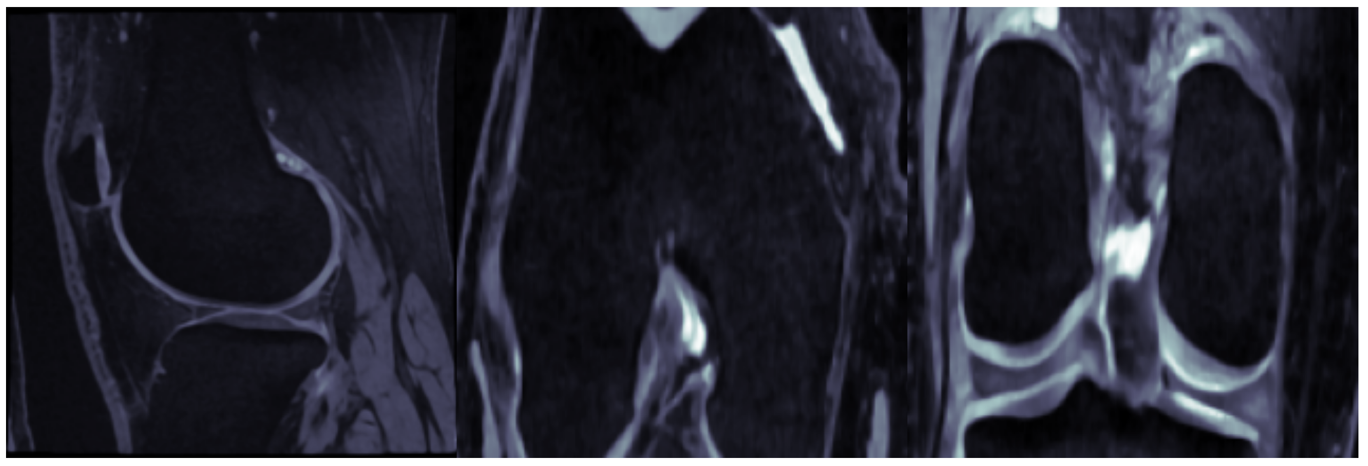
Figure 1. Demonstration of knee MRI in the three orthogonal planes (left to right): sagittal, coronal, axial.
Make 07 00094 g001
Figure 2. Overview of the general architecture of the proposed model. (a) Overall spatio-temporal structure of the data and network; (b) DyHGRU module comprising the encoder/decoder units, facilitating sequence-to-sequence learning; (c) MHGCN module integrating data balancing by HyGraphSMOTE, multi-view HGCN convolutions, and hypergraph structure learning (AHL).
Make 07 00094 g002
Figure 3. Synthetic node sequence generation process.
Make 07 00094 g003
Figure 4. Hypegraph GRU components: (a): Encoder component, (b): Decoder component.
Make 07 00094 g004
Figure 5. KOA incidence prediction performance under two criteria: (top) Δ K L definition; (bottom) Δ J S N definition.
Make 07 00094 g005
Figure 6. Clustered KOA incidence prediction performance under two criteria: (1) non to doubtful KOA ( P r o g r + ) and (2) non to moderate/severe KOA ( P r o g r + + ) . (top) Δ K L definition; (bottom) Δ J S N definition.
Make 07 00094 g006
Figure 7. Multi-step-ahead performance of longitudinal prediction of KOA progression under three distinct definition criteria (top to bottom: Δ K L ,   Δ J S N ,   Δ J S W ).
Make 07 00094 g007
Figure 8. Long-term predictions of KOA incidence and progression with respect to the baseline visit at + 5 , + 6 , + 7 follow-up times.
Make 07 00094 g008
Figure 9. KOA incidence and progression predictions for a specific knee in the OAI dataset. The first four images in each row correspond to the historic stage, while the latter four refer to the prediction stage. For the first two rows, dark orange and dark purple represent the tibial and femoral bones, respectively, while light yellow and light pink represent the corresponding cartilage structures. In the last row, the red part constitutes the femoral bone, while the light yellow represents the femoral cartilage. Top row—ground truth KL-grade sequence: 0 1 1 2 2 3 3 4 /Predicted KL-grade sequence: 0 1 1 2 2 3 4 4 . Medium row—ground truth KL-grade sequence: 1 1 2 2 2 3 4 4 /Predicted KL-grade sequence: 1 1 2 2 2 3 4 4 . Bottom row—ground truth KL-grade sequence: 0 1 1 2 3 3 4 4 /Predicted KL-grade sequence: 0 1 1 2 3 3 4 4 (green indicates correct prediction, red indicates erroneous prediction).
Make 07 00094 g009
Figure 10. Relative performance cost reduction and computational burden reduction for each major module of the overall model ablated. Left: Incidence; Right: Progression. Results reported for P = 3 .
Make 07 00094 g010
Figure 11. Performance of KOA incidence (dark blue) and progression (dark red) prediction performance under different sizes of encoder/decoder dimensionality d.
Make 07 00094 g011
Figure 12. Parameter importances for the incidence (left) and progression (right) tasks, respectively ( P = 4 cases).
Make 07 00094 g012
Table 1. Evaluation criteria for the various KOA Incidence and Progression tasks used in this study.
Inclusion Set Evaluation Criteria
Incidence C i n c l = { 0 , 1 } ( K L 1 ) K L 2 Δ J S N 1 -
Progression C i n c l = { 2 , 3 } ( 1 < K L < 4 ) Δ K L 1 Δ J S N 0.5 Δ J S W 0.7
Table 2. Illustrating case of knee dataset balancing via HyGraphSMOTE, associated with a KOA progression task, using a historic depth of P = 2 . We show the distribution of KL grades for the non-progressors, the progressors, the synthetically generated knees, and the total number of knees at the different time steps of the historical stage.
t 0 t 1 t 2
No _ Prog . Prog . Synth . No _ Prog . Prog . Synth . No _ Prog . Prog . Synth .
0714509448 329479302 000
114411017729 9181002514 000
21102779524 678881451 19211127958
3000 513762434 1640874743
N ˜ 7263 7263 7263
Table 3. Hyperparameter search space and optimal selected values for both incidence and progression tasks (case P = 4 ).
HyperparameterSearch SpaceIncidenceProgression
λ p r e d [ 0.2 , 0.8 ] 0.3 0.4
λ t r n [ 0.2 , 0.8 ] 0.7 1 cm
l e a r n i n g _ r a t e [ 1 × 10 6 , 1 × 10 1 ] 1 × 10 4 1 × 10 3
N l a y e r s ( M H G C N ) [ 1 , 2 , 3 , 4 ] 43
N l a y e r s ( C S h a p e N e t ) [ 1 , 2 , 3 , 4 ] 42
b a t c h _ s i z e [ 12 , 512 ] 25664
N h e a d s ( a t t n ) [ 4 , 16 ] 84
h m s o t e α [ 0.8 , 1.2 ] 0.9 1.1
d ( e n c ) [ 32 , 512 ] 256128
d ( d e c ) [ 32 , 512 ] 25664
Table 4. Literature overview of KOA incidence prediction works. Abbreviations: [H.: hospital, LU: Lund University, Dem.: demographics, Tbf.: tibiofemoral, hist.: history, CHECK: cohort hip and cohort knee].
MethodDatasetSourceInclusion SetDefinitionPred. TargetResults  ( AUC )
Guan et al. [7]OAIX-ray + {Dem., Injury hist., Tbf. angle}Baseline Δ J S W 1 J S W at + 4 0.857
Pedoia et al. [8]OAIMRI 0 K L 1 K L 2 K L 0.83
Alexopoulos et al. [9]OAIMRI 0 K L 1 K L = 2 K L at + 2 1 c m 7
Du et al. [14]OAIMRI-- K L at + 2 0.76
Janvier et al. [21]OAIX-ray K L = 0 Δ K L 1 K L at + 4 0.73
Joseph et al. [11]OAIMRI K L 2 K L > 2 K L at + 7 1 cm7
Kerkhof et al. [13]Rotterdam H.Imaging variables K L 1 K L 2 - 0.79
Kinds et al. [12]CHECKX-ray K L 1 K L 2 K L at + 5 1cm9
Woloszynski et al. [22]LUMRI K L 1 Δ J S N 1 K L at + 4 0.75
ProposedOAIMRI + {Dem., Injury hist.} K L ( t P ) { 0 , 1 } Δ J S N 1 Δ J S N at ( + 1 , + 2 , + 3 , + 4 ) 0.82 ( + 1 ) , 0.88 ( + 2 ) , 0.92 ( + 3 ) , 0.95 ( + 4 )
K L 2 Δ K L at ( + 1 , + 2 , + 3 , + 4 ) 0.82 ( + 1 ) , 0.85 ( + 2 ) , 0.90 ( + 3 ) , 0.93 ( + 4 )
Table 5. Literature overview of KOA progression prediction works. Abbreviations: [LUH: Lund University Hospital, MOST: Multi-Center Osteoarthritis Study, FNIH: Foundation for the National Institutes for Health, POP: Prediction of Osteoarthritis Progression Study, Dem.: demographics, Tbf.: tibiofemoral, hist.: history].
MethodDatasetSourceInclusion SetDefinitionPred. TargetResults ( A U C )
Imjabbar et al. [15]OAIX-ray 1 < K L < 4 Δ m J S N . 5 KL at + 4 0.75
Imjabbar et al. [15]MOSTX-ray 1 < K L < 4 Δ m J S N . 5 KL at + 4 0.75
Guan et al. [7]OAIX-ray 1 < K L < 4 Δ J S W 0.7 KL at + 4 0.86
Janvier et al. [21]OAIX-ray 1 < K L < 4 Δ J S W 1 KL at + 4 0.77
Woloszynski et al. [22]LUHX-ray K L 2 Δ J S N 1 KL at + 4 0.77
Kraus et al. [19]PfizerX-ray 1 < K L < 4 Δ J S W 5 % KL at ( + 1 , + 2 ) 0.85
Kraus et al. [20]FNIHX-ray 0 < K L < 4 Δ J S W 0.7 KL at ( + 2 , + 4 ) 0.81
Kraus et al. [18]POPX-ray 0 < K L < 4 Δ m J S N 1 KL at + 4 0.79
Halilaj et al. [16]OAIX-ray-- K L at ( + 1 , + 2 ) 0.86
Schiratti et al. [23]OAIMRI1 cm ≤ J S N 1.1 Δ m J S N 0.5 J S N at + 1 1 c m 5
Panfilov et al. [17]OAIMRI, X-ray-- K L at ( + 1 , + 2 , + 3 , + 4 ) 0.76 ( + 1 ) , 0.72 ( + 2 ) , 0.70 ( + 3 ) , 0.74 ( + 4 )
ProposedOAIMRI + {Dem., Injury hist.} K L ( t P ) at { 2 , 3 } Δ J S W 1 Δ J S W at ( + 1 , + 2 , + 3 , + 4 ) 0.80 ( + 1 ) , 0.85 ( + 2 ) , 0.89 ( + 3 ) , 0.93 ( + 4 )
Δ J S N 0.5 Δ J S N at ( + 1 , + 2 , + 3 , + 4 ) 0.81 ( + 1 ) , 0.85 ( + 2 ) , 0.91 ( + 3 ) , 0.93 ( + 4 )
Δ K L 1 Δ K L ( + 1 , + 2 , + 3 , + 4 ) 0.81 ( + 1 ) , 0.85 ( + 2 ) , 0.90 ( + 3 ) , 0.94 ( + 4 )
Table 6. Average AUC score of KOA incidence (Inc.) and progression (Progr.) prediction tasks under expanding historical record with respect to various demographic clusters.
Gender Age BMI
MaleFemale 50 50 59 60 69 70 NormalPre-ObeseObese
Inc. P = 0 0.84 0.81 0.83 0.79 0.82 0.84 0.79 0.83 0.85
P = 1 0.87 0.83 0.85 0.86 0.86 0.83 0.82 0.88 0.85
P = 2 0.91 0.89 0.89 0.87 0.89 0.92 0.89 0.91 0.92
P = 3 0.93 0.92 0.92 0.92 0.93 0.94 0.92 0.95 0.93
Progr. P = 0 0.82 0.79 0.77 0.80 0.82 0.85 0.78 0.82 0.83
P = 1 0.87 0.83 0.80 0.83 0.87 0.89 0.82 0.85 0.88
P = 2 0.92 0.88 0.84 0.89 0.92 0.94 0.88 0.89 0.93
P = 3 0.94 0.92 0.89 0.93 0.96 0.97 0.92 0.94 0.96
Table 7. Table showcasing future KL progression predictions of knees in Figure 9 with respect to the previous time step.
Knee #1 (Top Row) Knee #2 (Medium Row) Knee #3 (Bottom Row)
+ 1 + 2 + 3 + 4 + 1 + 2 + 3 + 4 + 1 + 2 + 3 + 4
Actual ( + 0 ) ( + 1 ) ( + 0 ) ( + 1 ) ( + 0 ) ( + 1 ) ( + 1 ) ( + 0 ) ( + 1 ) ( + 0 ) ( + 1 ) ( + 0 )
Predicted ( + 0 ) ( + 1 ) ( + 1 ) ( + 0 ) ( + 0 ) ( + 1 ) ( + 1 ) ( + 0 ) ( + 1 ) ( + 0 ) ( + 1 ) ( + 0 )
Table 8. Average multi-step-ahead AUC performance of KOA incidence prediction under varying-size ( P ) of historical windows (with respect to KL grade). First column ( P 0 = { 0 } ) corresponds to results drawn from training and testing on data from the baseline visit alone, while subsequent rows progressively incorporate successive time points ( P 1 = { 0 , 1 } , P 2 = { 0 , 1 , 2 } ) , P 3 = { 0 , 1 , 2 , 3 } . First row indicates performance of the full proposed model. Subsequent rows indicate degradation of performance with respect to to the corresponding ablated component. Full model configuration: GRU + Demographics + SMOTE + Attention + Pre-training + Injury + SSL.
P = P 0 P = P 1 P = P 2 P = P 3
Full model configuration 80.74 % 83.62 % 87.13 % 92.45 %
w/o HyGraphSMOTE 5.28 % 6.02 % 4.96 % 5.33 %
w/o Demographics [all] 3.03 % 2.96 % 3.12 % 2.81 %
w/o Demographics [Age] 2.21 % 3.04 % 2.48 % 1.95 %
w/o Demographics [BMI] 1.95 % 2.44 % 3.05 % 2.13 %
w/o Demographics [Gender] 1.18 % 1.26 % 2.11 % 1.47 %
w/o Injury 1.61 % 2.03 % 2.18 % 1.79 %
w/o SSL 5.17 % 6.39 % 7.02 % 6.82 %
w/o Pretraining 3.09 % 4.13 % 5.27 % 4.85 %
w/o ACT 7.18 % 6.06 % 5.70 % 6.43 %
Table 9. Average multi-step-ahead AUC performance of KOA progression prediction under varying-size ( P ) of historical windows (with respect to KL grade). First column ( P 0 = { 0 } ) corresponds to results drawn from training and testing on data from the baseline visit alone, while subsequent rows progressively incorporate successive time points ( P 1 = { 0 , 1 } , P 2 = { 0 , 1 , 2 } ) , P 3 = { 0 , 1 , 2 , 3 } . First row indicates performance of the full proposed model. Subsequent rows indicate degradation of performance with respect to to the corresponding ablated component. Full model configuration: GRU + Demographics + SMOTE + Attention + Pre-training + Injury + SSL.
P = P 0 P = P 1 P = P 2 P = P 3
Full model configuration 82.19 % 86.41 % 91.37 % 95.16 %
w/o HyGraphSMOTE 5.75 % 6.68 % 7.33 % 6.59 %
w/o Demographics [all] 2.80 % 4.11 % 4.09 % 3.38 %
w/o Demographics [Age] 2.75 % 3.49 % 2.08 % 3.05 %
w/o Demographics [BMI] 2.39 % 2.88 % 3.11 % 2.98 %
w/o Demographics [Gender] 1.02 % 1.22 % 1.74 % 2.02 %
w/o Injury 0.98 % 1.83 % 2.17 % 2.64 %
w/o SSL 5.92 % 7.06 % 6.27 % 5.75 %
w/o Pretraining 4.41 % 6.08 % 5.14 % 4.55 %
w/o ACT 6.22 % 7.17 % 6.44 % 7.08 %
Table 10. Number of trainable parameters and computational cost by component per single forward pass (progression task).
ComponentParameters (Inc.)Percentage (%)Parameters (Progr.)Percentage (%)
C_Shape.Net1,072,42126.67%943,97252.39%
MHGCN1,755,94043.68%468,90026.02%
Encoder185,8564.62%74,4964.13%
Decoder739,46118.37%246,65813.70%
ACT266,2406.66%67,5843.75%
Total 4 , 019 , 918 100 . 0 % 1 , 081 , 610 100 %
Table 11. Averaged multi-step-ahead comparative performance of KL longitudinal prediction of KOA incidence and progression under varying-size ( P ) of historical windows. Metric: balanced accuracy ( A U C ).
Incidence Progression
P = 0 P = 1 P = 2 P = 3 P = 0 P = 1 P = 2 P = 3
DyHRM 0.82 0.85 0.90 0.93 0.81 0.85 0.90 0.94
TFT 0.74 0.81 0.87 0.91 0.76 0.81 0.88 0.93
TCAN 0.76 0.80 0.84 0.87 0.77 0.79 0.85 0.88
AGCRNN 0.77 0.81 0.83 0.86 0.79 0.78 0.86 0.87
Disclaimer/Publisher’s Note: The statements, opinions and data contained in all publications are solely those of the individual author(s) and contributor(s) and not of MDPI and/or the editor(s). MDPI and/or the editor(s) disclaim responsibility for any injury to people or property resulting from any ideas, methods, instructions or products referred to in the content.