Article

Full Domain Analysis in Fluid Dynamics

1
Institute of Technology, Resource and Energy-Efficient Engineering (TREE), Bonn-Rhein-Sieg University of Applied Sciences, 53757 Sankt Augustin, Germany
2
Autodesk Research, 53111 Bonn, Germany
3
Department of Mechanical Engineering, University of Siegen, 57068 Siegen, Germany
4
Fraunhofer Institute for Algorithms and Scientific Computing (SCAI), 53757 Sankt Augustin, Germany
*
Author to whom correspondence should be addressed.
Mach. Learn. Knowl. Extr. 2025, 7(3), 86; https://doi.org/10.3390/make7030086
Submission received: 3 June 2025 / Revised: 4 August 2025 / Accepted: 14 August 2025 / Published: 18 August 2025

Abstract

Novel techniques in evolutionary optimization, simulation, and machine learning enable a broad analysis of domains like fluid dynamics, in which computation is expensive and flow behavior is complex. This paper introduces the concept of full domain analysis, defined as the ability to efficiently determine the full space of solutions in a problem domain and analyze the behavior of those solutions in an accessible and interactive manner. The goal of full domain analysis is to deepen our understanding of domains by generating many examples of flow, their diversification, optimization, and analysis. We define a formal model for full domain analysis, its current state of the art, and the requirements of its sub-components. Finally, an example is given to show what can be learned by using full domain analysis. Full domain analysis, rooted in optimization and machine learning, can be a valuable tool in understanding complex systems in computational physics and beyond.

Graphical Abstract

1. Introduction

Problem-solving in fluid dynamics is a major research and development field with a large impact on our energy usage as well as a significant potential to make our society more sustainable. Due to the complexity of the field, creativity and innovation can be highly challenging. Only by increasing our understanding of entire problem domains can we systematically discover innovative solutions and reduce the risk involved in early decision-making. Algorithms must therefore address this need for innovation and risk reduction.
This work, therefore, introduces full domain analysis (FDA): the ability to efficiently understand the full space of solutions (e.g., shape designs) in a problem domain and analyze the behavior of those solutions in an accessible and interactive manner. FDA does not refer to a specific method but rather to a methodological framework that specifies which components are required when analyzing expensive domains in a structured fashion. The term “full” refers to the goal of achieving a comprehensive understanding of the solution space, rather than a claim of exhaustive enumeration, which is often computationally intractable. Applying FDA to problem domains in fluid dynamics requires taking into account the particularities of flow behavior and inefficiencies of fluid simulations. Small changes in flow environments can have significant and non-local effects on the airflow. If we want to understand these effects, we need efficient methods and frameworks to predict relevant flow features in a large diversity of settings (e.g., shapes). We also need to be able to represent this understanding in a concise manner, to reduce the cognitive load on engineers analyzing such complex domains.
Assuming engineers are only interested in solutions that are optimal w.r.t., some measure, the following questions must be answered to realize this goal:
  • How should designs be encoded to allow for efficiency in both determining solution quality and diversity of solutions?
  • How can a large, diverse set of solutions be created efficiently?
  • How do we incorporate and/or discover characteristics that produce well-performing designs of shapes?
  • How can users understand and navigate large design spaces?
In the field of artificial intelligence, specifically optimization and machine learning, a new body of work has emerged that enables the automation of creative processes that were classically only possible within the capabilities of the human mind. This trend reflects the growing consensus on the potential for machine learning to fundamentally enhance fluid mechanics research [1], creating new opportunities for design and analysis that frameworks like FDA aim to structure.
Methods like deep generative models (see [2]) and divergent optimization (see [3]) now exist that enable generating large sets of innovative solutions. The ability to generate many different, high-quality solutions to a problem domain in an efficient manner represents a significant step towards FDA and improving our ability to understand and reduce the unwanted consequences of design decisions.
In this work we explore synergistic effects of state-of-the-art evolutionary optimization, surrogate modeling techniques, and deep learning applied to the automated design of structures in the domain of fluid dynamics. We present an FDA framework and tool set that allows us to better explore and understand fluid dynamics design and develop automated design methods.
Figure 1 shows the FDA framework from the perspective of the user process. The goal of FDA is to get a representative set of flow features and flow manifestations around a large number of possible shapes in a predefined environment. It is defined as an iterative process that is started by the user defining parameters, constraints, and objectives that define the problem domain (1). Based on this, an efficient generative algorithm then creates a large variety of designs (2). The user then examines the design performance and characteristics (3) and can decide to select promising design regions, or design classes (4). Based on this selection, which can be modeled to understand user preferences (see [4]), parameters, constraints, and objectives can be adapted, after which the FDA process starts its next iteration. This allows a user to quickly get an overview of what designs perform well and zoom in on or recombine design regions.
Machine-learning techniques are used to guide iterative experimentation with novel designs. The major contribution of this work is to provide a framework that describes the goal and requirement set of FDA and its components: encodings (the manner in which we encode, or parameterize, the configuration of a flow domain), search, CFD, efficiency, and visualization. We provide examples of state-of-the-art methods that are able to fulfill these requirements. The following FDA components are discussed in this work:
  • Encoding of solutions;
  • Effective and efficient divergent search;
  • Fast CFD solver that supports accurate flow for diverse shapes;
  • Statistical learning methods to efficiently sample and predict characteristics of solutions;
  • Machine learning methods that learn characteristics and representations of solution sets.
The examples of FDA components can be used independently but all belong to an ecosystem of FDA methods. Most of this article gives examples of components and their application to the domain of shape optimization in fluid dynamics. We also elaborate on their shortfalls and future work arising from the requirements of FDA. The next sections discuss novel methods that, together, solve the problems mentioned here. Section 2.1 specifies free-form as well as data-driven shape encodings that provide the search space. The encodings are used to find diverse solution sets, described in Section 2.2. Section 2.3 describes the requirements of simulation environments when evaluating diverse shape sets. The matter of algorithmic efficiency, a key element of FDA, is considered in Section 2.4. A fully implemented example of what can be achieved with FDA is given in Section 3. Finally, we provide recommendations about future work involving FDA methods in Section 4.

2. Materials and Methods

2.1. Encodings

A generative design system requires an in silico representation of the design problem and its prospective solutions. In the context of the work herein, this requires encoding shapes. Several intuitive encodings exist, all with their own benefits and problems. It is tempting to encode the coordinates of such a free shape directly into the search space, as this can result in all possible shapes. However, this approach would require a large number of parameters, increasing the dimensionality of the search space, and producing many invalid shapes due to intersecting outlines. These problems can be circumvented by parameterizing certain characteristics of a basic shape, which was derived, for instance, in the design optimization of airfoils (see [5]). However, such basic shapes might not exist for many areas of design where components are customized to create mechanisms that meet specific path and force characteristics. Therefore, there are several factors to consider when choosing a shape representation. This research emphasizes search space dimension, coverage, validity, and navigation of encodings. In what follows, we define requirements of encodings and discuss whether and how common encodings fulfill these requirements.

2.1.1. Requirements

In optimization, solutions are usually encoded by a number of real-valued parameters, i.e., parameter space X (see Figure 2). x X is a vector that is transformed into the final shape s by some expression method e, which we will discuss hereafter. The full solution space S represents the vector space containing all possible solutions. This separation between X , therein called a genetic space, and a phenotypic space S , is a common and explicit practice in evolutionary computation (see [6]). By independently treating these spaces, we can investigate more readily the various encodings, the translation between X and S , and the encodings’ constraints. For fluid flow around obstacles or shapes, these shapes are elements taken from the solution space S , subject to high spatial (and possibly temporal) resolution. Therefore, S is usually of much higher dimensionality than the parameter space X . Encodings aim to reduce this dimensionality with a function that maps a low-dimensional search space X to a reachable manifold R in S with d i m ( R ) d i m ( S ) . Only points on R can be reached by points in X .
In the following, we define requirements for and examples of encodings, describe their strengths and weaknesses, and make recommendations for further research.
Reachability
Create a wide variety of designs, maximizing the reachable region, or its coverage of the valid solution space V . The quality of an FDA method relies on the ability to reach as many solutions as possible. The reachable solution space R contains all reachable in situ solutions. S contains all possible valid solutions and invalid solutions. The goal is to maximize R , w.r.t. the solution space S . If the encoding itself cannot produce certain solutions that are valid and desirable, due to a misalignment between user intent and the formal encoding, FDA will systematically miss those desirable solutions. The requirement on reachability or completeness (see [7]) aims for the encoding to guarantee a maximal degree of freedom in order to avoid unnecessary constraints on the phenotype space.
Validity
Minimize the number of invalid solutions on R . Often, a number of reachable and/or unreachable solutions are also invalid, e.g., when these shapes can or should not be manufactured due to limitations in machining or design. Although we want to understand invalid solutions as well, we mostly want to be able to avoid reaching them. The number of invalid solutions in S can be much greater than V . It is not possible to evaluate invalid solutions, and so we cannot calculate their fitness value. Hence, the navigation through the search space X would be impossible or at least ineffective (see [8]). In FDA, a primary goal of an encoding is to maximize the reachable manifold R w.r.t. the valid subspace V , which can contain multiple unconnected regions. To ensure that the reachable manifold R does not contain any invalid solutions, constraints can be applied to X . Adding constraints can be tedious and usually needs multiple iterations, depending on the complexity of the encoding’s mapping. It is preferred that the encoding find a manifold that contains as many valid and as few invalid solutions as possible, without the need for constraints.
Searchability
Minimize dimensionality ambiguous w.r.t. sensitivity. The encoding provides the search space X for optimization. The solution space S suffers from the curse of dimensionality, a term coined by Bellman [9]. It dictates that the relative difference of the distances of the closest and farthest data points goes to zero as the dimensionality increases. This phenomenon already occurs at low numbers of dimensions, which was shown by Beyer [10]. We therefore prefer compactness (see [7]) of X to minimize its dimensionality and increase search performance.
According to authors like Olhofer [7], small steps in X should lead to small steps in S . Encodings that disobey this rule are coined sensitive (see [11]). However, the sensitivity of an encoding can help find diverse shapes by allowing a search algorithm to jump around in S and find disconnected high-fitness regions. Making use of lower-performing solutions as stepping stones towards better solutions, some evolutionary optimization algorithms are able to produce high-diversity solution sets (see [12]). So while the dimensionality of X should be kept low, it remains an open question whether sensitivity is preferable in divergent search. Some evidence exists that it might be beneficial in the context of FDA.
Predictability
Allow for efficient search using predictive models. Efficient search in the fluid dynamics domain usually encompasses predictive models that allow us to replace some expensive evaluations, i.e., the use of a CFD solver. The encoding itself needs to be suitable for use with predictive (machine learning) models. This is done by learning to predict a function x f ( x ) , where f is a fitness function that determines the quality of a solution based on its parameters x. Sensitive encodings (i.e., small steps in X produce large steps in S ) are usually harder to predict accurately, as large steps in S can entail large qualitative changes. However, in this case, large steps might still be easy to model for monotonous transformations, e.g., when a large step just means that the shape is increased in size. Especially when the air flow changes in a qualitative manner, the modeling problem becomes more difficult, requiring more samples from simulation, more complex models, or slower model conversion. Local models, e.g., those that are commonly used in optimization, might become too complex if used in FDA. Hence, it might be more beneficial to use models that approximate the entire design space.
Human Understanding and Effort
Allow engineers to understand the domain and the implications of their definition. Minimize effort to define the domain. Minimize effort to use the results in production. Domains in fluid dynamics require significant effort to formally define and code. In classical optimization, e.g., airfoil or wing design, the variety of possible shapes is often confined by a priori design decisions. These design decisions are part of the encoding formalization process. In FDA for fluid dynamics, we aim to enhance the engineer’s intuition, i.e., maximize the diversity of solutions and enhance the engineer’s understanding of how morphological and flow features are correlated. We therefore might prefer encodings that have more degrees of freedom and a larger range of possible solutions s S than what is common in fluid dynamics optimization. Identifying theoretical solutions is only the initial step towards realizing them in the real world. Solutions that are defined in industry-compatibly formats could be preferred. The encodings should allow engineers to understand, fine-tune, and realize in the real world.
Prior Examples
Support learning from prior examples. In large and complex domains, we might want to be able to insert prior knowledge about known working solutions to initiate FDA.

2.1.2. State of the Art

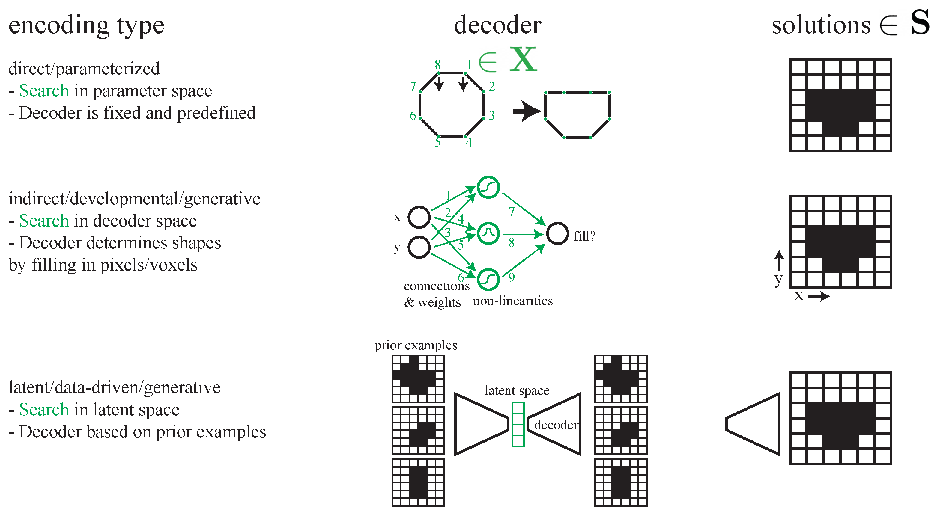
We now discuss various encodings (see Figure 3), their qualities w.r.t. the requirements from Section 2.1.1, and the implications for FDA.
Direct/Parameterized
Direct, or parameterized, encodings are the most common approach, defining a solution s based on a vector of parameters that is decoded into a shape. The parameter space X , shown in green in Figure 3 (top), usually consists of the coordinates and/or weights of deformation nodes around a base shape. A naive approach is to directly control the shape’s nodes. Other examples are airfoils (see [13]), splines (see [14]), or FFD of a base shape (see [15]). Sarakinos [16] showed that FFD can better compress X in fewer dimensions than spline representations. Reachability in S is limited by the hand-designed decoding, applying a parameter tuple to the user-selected base shape. Limited preliminary understanding of the domain can make it hard to define a decoder in the first place. In contrast, a high degree of experience might lead to a more conservative stance, using well-understood decoders even when innovation is sought after. The validity of shapes can be influenced by putting constraints on the parameters. Constraints can be easy to implement, but a large effort might be required to understand how constraints affect the reachable region R . In FDA, we want to avoid constraints initially. If X contains large regions of invalid solutions, constraints might be necessary to allow FDA to be useful. However, careful consideration is necessary to avoid excluding desirable solutions. Searchability of direct encodings is given by the simple tuple structure of their parameters. The low dimensionality of X makes the search problem easier. Predicting a parameterized solution’s quality is well understood. The encodings can be used in efficient optimization schemes like Bayesian optimization, which will be explained in Section 2.4. For complex solution structures, a higher-dimensional X is necessary, which can render the necessary effort to design a proper encoding prohibitive. It is easy to understand the solutions in S that will be reached, but hard to understand what regions are missed and whether they contain interesting solutions. However, once artifacts that solve the problem are found, transferring them to the real world is easier. The engineer can control transferability through the decoder directly. Translating prior examples into the encoding is usually done through shape matching. Shape matching is a research area that focuses on matching a prior shape using an encoding with an optimization algorithm (see [17]).
Indirect, Developmental, and Generative Encodings
Indirect (also called developmental or generative) encodings (Figure 3, center) perform search in the decoder space. Both the structure and weights of a neural graph, a common representation of a decoder called CPPN (see [18]), can be changed. A solution in S is created by the CPPN by receiving the locations of pixels or voxels and returning whether that location is part of the solution or not. Gaier [19] showed that CPPNs can be used to express NURBS, which makes indirect encodings more suitable for engineering applications. A single change in a search dimension may lead to multiple qualitative changes of the solution (see [8]). An indirect approach can be used to reduce the number of search dimensions necessary to describe a wide variety of shapes. Indirect encodings can outperform direct encodings due to the reduction of the dimensionality of X (see [20]). Kicinger [21] and Clune [22] showed that indirect encodings work especially well when problem regularity increases, as regularity can be modeled by simple activation functions in the neural representation. Other interpretations include the use of a Fourier series to encode the genes of a closed curve. Yannou [23] used this method to create car silhouettes with a fixed-dimensionality X . The decoder can generate shapes in any resolution, helping to overcome the problem of maximizing the reachable solution region R while using a low-dimensional X . By combining only a few elements of the decoder, a wide variety of shapes can be reached, as was shown in Clune [24]. CPPNs are difficult to constrain due to the complex expression function, but efforts have been made by including a post-processing step for CPPN results (see [25]). Regularities, like symmetry, can be injected by adding Gaussian building block functions into the CPPN. CPPNs are usually optimized using non-gradient-based evolutionary algorithms that are able to handle the fact that they can change structure and the unavailability of gradients (see [26,27]). Successful steps have been taken to connect graph structures like CPPNs to efficient predictive models (see [28,29,30,31]). CPPNs, which can change their internal structure and require a forward pass of pixel or voxel coordinates through the graph network, complicate the understanding of their expression, and researchers typically have to rely on post-hoc analysis of the resulting solutions. Again, similar to direct encodings, we need to use search algorithms to match prior examples using the encoding. Clune [24] showed that CPPN representations can be matched to shapes.
Latent-Generative
More complex search spaces can make FDA an inefficient or even infeasible task. Indirect encodings are a very flexible method for the problem of defining decoders (see [26,27]). However, S might be simply too vast and complex and contain too many locally optimal solutions for non-data-driven techniques to be efficient and effective. Although shape matching is a viable method to find prior examples with indirect encodings (see [24]), the encodings themselves are not trained in a data-driven manner. The advent of GMs circumvents the step of evolving an encoding and uses highly efficient machine learning techniques to represent large numbers of prior examples, instead, a topic reviewed by Regenwetter [32]. Figure 3 (bottom) shows an example of such a GM, a VAE that consists of two neural networks [33]. The first, the encoder, compresses high-dimensional shape sets to a low-dimensional (latent) representation. The second network, the decoder, decompresses the latent space back into the original high-dimensional shape. Training is performed using a loss function on the decoder’s output shape, comparing it with the training input. Regularization terms can be added to increase the regularity of the latent space. Alternative interpretations of GM are GANs, which use similar networks but train them in an adversarial manner. Here, the decoder, called the generator, attempts to generate realistic examples that are not contained in the training set. The encoder is changed into a classifier called the discriminator, which is responsible for distinguishing real from generated examples.
The compact design space provides an excellent search space in FDA. The decoder has the potential to capture more relevant design characteristics than those human designers would suggest (see [34]). The authors showed that GM can even allow local geometry modification in a 3D car design problem. GMs can interpolate between training shapes or find new combinations of those shapes to produce innovative, novel solutions. In another example, GANs have been used to synthesize aerofoils as well (see [2]).
Reachability with GMs is an incredibly hard problem to analyze, depending on the dimensionality of the latent space, which is directly connected to the accuracy of the reproduced training shapes. While the state-of-the-art in image generation produces a very realistic diversity of images, it is not easy to determine the exact structure of R , except by trial-and-error or search in the latent space. The GM is constrained to produce interpolations or new combinations of training shapes. At the same time, these constraints create blind spots in areas the data set does not cover. However, GM might reach human blind spots, finding more innovative solutions through data-driven discovery. Hagg [35] showed that in some cases, direct encodings might outperform GM in an FDA setting, where the dimensionality of the parameterized and latent encodings was the same. Especially, the diversity of output in a multisolution context was shown to be higher for direct encodings.
Constraints are not easy to implement, as GM will just learn a representation based on the data it is presented with. Validity has to be injected by using a data set consisting of valid shapes. Bentley [36] shows that constraints on the training data can enable learning latent representations that produce mostly valid shapes. They use a GA to create a valid data set, which shows that an initial data set is necessary, which can be intractable to create for expensive optimization problems. Without a data set, a GM cannot be trained, but in order to efficiently create the data set, expensive computational effort is needed to optimize the problem in order to find valid data points. A posterior inclusion of constraints usually has to be accomplished through post-processing or by retraining or adjusting the model by example. An example of such a retraining was shown by Hagg [11], where the user was able to deselect solutions offered by the GM.
The latent space provides a dimensionality reduction that makes search more feasible. The space itself, if trained in a regularized manner, can be continuous and smooth by adding priors on the latent distribution. Examples have appeared in the very recent past that show we can predict the performance of points in the latent space of a GM with efficient models, either neural networks (see [37]) or GPs (see [38]). The technique is quite new, and its effectiveness probably depends on the smoothness of the latent space. The ability to understand the decoder in latent encodings is part of the bigger question of understanding neural network models. Explainability has become its own subfield and does not limit itself to “analysis-by-example”. Disentangling the latent dimensions of a VAE makes it easier to understand the latent space for humans (see [39]). Some work has been done on GMs that produce simulation-ready meshes Rios [40]. This decreases the effort of integrating a GM into real-world design and production processes.
Inserting prior knowledge about solutions is the entire idea of GM. By learning representations from data, algorithms are fed with known good solutions, including prior knowledge of good and acceptable solutions, into the model, automatically. The usually large data sets of known prior solutions have to be transformed into a digital form that serves as training input to GMs. Examples of such transformations are scans of analog objects or technical drawings that are translated into a discretized bitmap or voxel representation. These representations can be presented to the GM during training.

2.1.3. Discussion

An overview of this section is presented in Table 1.
Direct encodings are well-understood but have the potential to limit the reachability of solutions. Indirect encodings, although having the potential to create more innovative shapes, are hard to predict and therefore can make them less efficient in the engineering context. Latent encodings have a large potential and are efficient, but their performance is constrained by the number of data points available a priori. Simultaneously, being able to derive an encoding only based on data can help us circumvent the problem of having to manually design an encoding and extract it from the data directly. Recent work leverages diffusion-based generative models to sample aerodynamic shapes directly in latent space. DiffAirfoil employs a latent-space denoising diffusion model that produces realistic, constraint-aware airfoils from only ≈2000 training examples [41]. Airfoil Diffusion extends this idea to conditional generation on target lift and drag coefficients [42]. For 3D structures, VehicleSDF combines DeepSDF with a surrogate-aided optimization loop to generate drag-aware car geometries [43].
Implicit Neural Representations (INRs) have matured into powerful shape priors. StEik [44] stabilizes SDF training for high-detail objects, while NeuVAS [45] adds variational editing under sparse curve constraints. INR-based topology optimization frameworks such as TOINR [46] now rival classical level-set methods.
Finally, disentangled latent learning has become a key tool for explainable encodings. Isometric diffusion enforces an isometry between latent and solution spaces, leading to controllable semantic axes [47]. NashAE shows that adversarial covariance minimization disentangles latent factors without prior knowledge of factor count [48].
Please refer to [49] for an insightful comparison of various encodings in the context of multisolution search algorithms.

2.2. Search

We now discuss the question of how to use encodings to create diverse solution sets. In FDA, the goal is not so much to come up with a valid, global optimum but to understand the diversity of solutions and provide a more exploratory framework. This can lead to efficiency problems, because a large part of X might be less interesting to the user. The search might spend too much time producing invalid solutions or even never reach valid regions. On the other hand, invalid solutions can be accepted as stepping stones to valid regions (see [12,50]). To create these solutions, we can employ optimization algorithms. In fluid dynamics and efficient FDA, although we might indeed want to understand as much about the domain as possible, we usually observe domains under the light of some definition of optimality. Optimality is defined as the objective to minimize a function f on a solution, which determines the quality of a solution.
Common objectives in fluid dynamics are to minimize the drag force or the amount of turbulence in a flow caused by a shape. In these cases, we are not interested in all shapes that we can produce in a domain but at least those that perform well according to the fitness function. A performance function f ( x ) that formalizes the optimization goal is defined based on the objective. The (unconstrained) optimization problem is therefore defined as follows:
x m i n = arg min x ( f ( x ) )
where x m i n is the global minimizer (or location of the minimum) of the function f ( x ) . f ( x ) is the fitness value at x. A parameter tuple x is mapped to a solution s via a commonly user-defined encoding function or method e. The encoding e usually entails computer code that determines the output format of a solution.
The goal of most classical optimization algorithms is to find a single, optimal solution. This objective is incongruent with the goal of FDA, which is to understand as much about a domain as possible. To determine how different solutions actually solve a problem requires generating a large variety of designs. We therefore adapt Equation (1) to output a set of locally optimal solutions X m i n , l o c , which can contain the global optimum x m i n .
In order to produce X m i n , l o c , we cannot merely define the fitness function and search for a minimizing (or maximizing) parameter tuple. We need to introduce a way to determine when we add a solution to the solution set. If we cannot make such a determination, the problem is malformed, as we could produce any number of randomly selected solutions. Commonly, for solution selection, a criterion is used that takes the form of a threshold function, which would allow any solution below the threshold to be added to the solution set. The multisolution optimization problem is defined as follows:
X m i n , l o c = arg min x ( f ( x ) ) , | x i x | ϵ
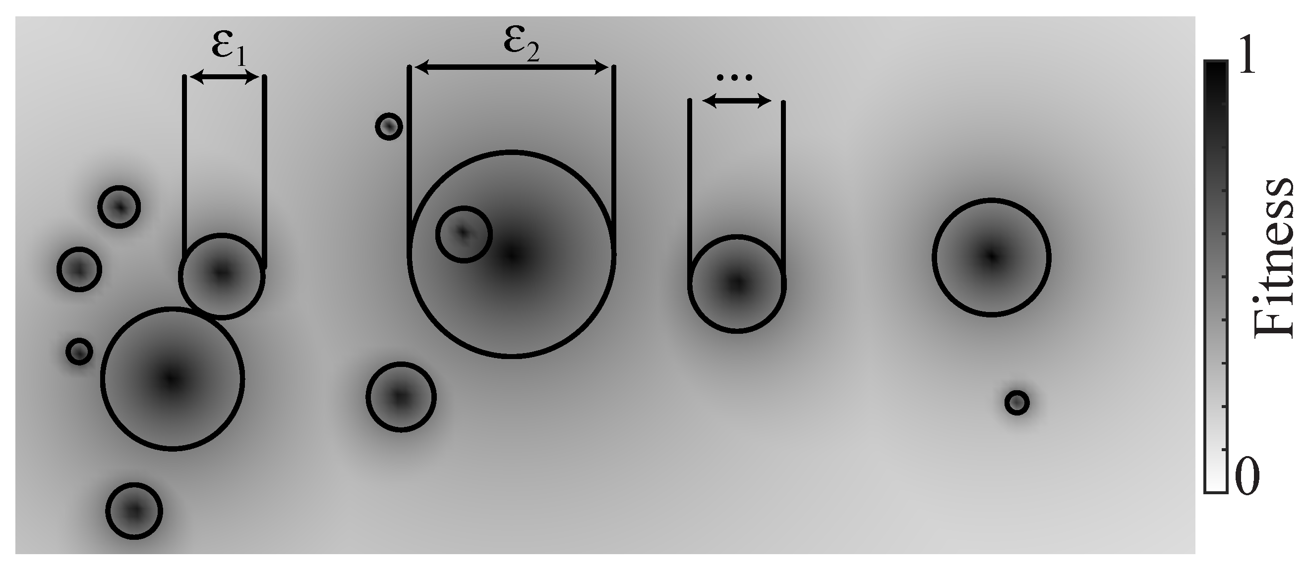
where X m i n , l o c is the set of solutions that minimizes f ( x ) in a local neighborhood, a niche. A niche is defined by a distance-based metric ϵ on the parameters. ϵ is a domain-dependent parameter and might not be constant within the same domain, which can be observed in the heterogeneous fitness landscape in Figure 4. In Equation (2), ϵ also serves as a proxy for a value that may be determined explicitly, implicitly, or dynamically.
What follows are the requirements for optimization algorithms used in FDA.

2.2.1. Requirements

In the following, we define requirements to optimization algorithms and examples of methods, describe their strengths and weaknesses, and make recommendations for further research.
Multiple Solutions
The search should return multiple solutions. To analyze an entire domain, optimization algorithms should only be considered if they return multiple solutions. Single-solution algorithms do not provide an overview of the solution space S . The search algorithm should fulfill Equation (2).
Coverage
Search should maximize solution diversity. As we are interested in finding “all” solutions in a domain, the search method used in FDA should cover as much of the solution space S as possible. As the search algorithm can only reach those points in S that are reachable by the encoding, we can simplify the requirement for search to maximize the coverage in X .
Diversity
Diversity of the solution set should be high. In FDA, we are not only interested in finding as many solutions as possible or maximizing the spread in the search space. Much more appropriately, we want to create a diverse set of solutions that maximizes the knowledge gain of the user and is a good representation of the variety of solutions. Two aspects are of importance here: how we compare solutions and how well the space containing those solutions is sampled. Hagg [51] discussed two aspects of diversity: the uniformity of the distribution of solutions (discrepancy) spread (see last section) or a combination of the discrepancy and spread (coverage). Comparing solutions in S rather than X prevents genetic neutrality. Neutrality is the phenomenon where multiple solutions in X are mapped to the same solution in S . Neutrality degrades diversity and diversity metrics (see [51]). Within the space covered by the search, solution diversity might be equally important to the user. For a review of diversity metrics, see [52].

2.2.2. State of the Art

In multisolution optimization, we distinguish three candidate paradigms for FDA, MOO, MMO, and QD, each having a different idea behind the selection criterion.
Multiobjective Optimization
MOO (see Figure 5a) aims to produce different trade-offs between multiple optimization criteria. The selection criterion selects a solution when it performs better w.r.t. one of the optimization criteria. The resulting Pareto front of solutions represents the trade-offs between multiple objectives. Solutions are diverse w.r.t. this trade-off, yet not to their behavior or morphology. The most successful methods to date are the NSGA-II (see [53]), the strength-Pareto evolutionary algorithm (SPEA) (see [54]), and the s-metric selection evolutionary multiobjective optimization algorithm (SMS-EMOA) (see [55]).
Multimodal Optimization
Niching, a concept from evolutionary optimization that protects solutions if they outperform close-by alternatives, is a concept that goes back to the 70s (see [56,57]). The idea was used to increase the performance of single-objective evolutionary optimization first. Multisolution optimization came along almost two decades later. The use of niching was now used to increase the number of output solutions of evolutionary algorithms. Various algorithms have been introduced, like basin hopping (see [58]), nearest-better clustering (see [59]), and restarted local search (RLS) (see [60]).
In MMO (see Figure 5b), sets of solutions are created that spread out over the search (parameter) space and find as many (local) optima as possible. Here, the selection criterion selects a solution when its location in X is far enough away from other known locations or its quality is higher than that of a close solution.
Quality–Diversity
QD optimization solves the problem
X m i n = arg min x ( f ( x ) ) , | p ( x i ) p ( x ) | ϵ
where X m i n is the set of solutions that minimizes f ( x ) in a local neighborhood, a niche, defined by ϵ on the phenotypic characteristics considered by the function p ( x ) .
Finally, QD (see Figure 5c) is a novel paradigm that aims to find a large diversity of high-performing solutions (see [61]). In QD, diversity is defined in terms of the behavior or morphology of solutions, ignoring the diversity in parameter space altogether. In QD, the selection criterion is similar to that of MMO, except that locality is determined based on behavior or morphology, in S , not in X . QD was originally created to generate many walking gait strategies for a hexapod robot, allowing for quick restrategizing when the robot was damaged. The behavioral characteristics describing the niche space were manually defined and well-suited for the purpose of generating strategies that used the robot’s six legs in varying degrees. Instead of manually defining features, which can be an intricate task, QD has been combined with latent-generative models (see [11,35,62,63]). The generative models can either be used as a latent-generative search space (see Section “Latent-Generative”) or as a feature/characteristic space, driving diversity of solutions and enabling the discovery of representative prototypes (see [64]). The resulting feature models encode characteristics that can be used to define QD’s archive dimensions. The drawback of such a purely data-driven approach is the lack of control over what solutions are found and how they are laid out to be compared with each other. A combination of data-driven and manually defined characteristics has not been researched in any work, to the knowledge of the authors of this work.
Recently, several algorithmic advances have closed the efficiency gap between QD and classical optimization. Differentiable QD (DQD) exploits objective and descriptor gradients; MEGA and CMA-MEGA achieve order-of-magnitude speed-ups on continuous tasks [65]. In latent spaces, latent-consistent Bayesian optimization (LCA-LSBO [66] and CoBO [67]) increases sample efficiency by regularizing VAE embeddings. Bayesian QD variants such as BOP-Elites combine BO acquisition functions with MAP-Elites archives [68]. These contributions demonstrate that QD can scale to 10–100× higher-dimensional problems than the 2018 state of the art, surpassing many conventional Representation-Surrogation-Optimization loops.

2.2.3. Comparison of Paradigms

The three paradigms were analyzed and compared by Hagg [51]. The analysis showed that the diversity of solution sets produced by the three paradigms differs greatly. QD results in the highest diversity of solutions, making it an appropriate optimization method for FDA. Although MOO has been widely used to create multiple solutions in one go, solution diversity is only defined based on the trade-off between objectives. This trade-off does not address diversity in terms of how a solution solves a problem, making it less appropriate for FDA in early design phases. While QD’s resulting diversity is highest among the paradigms, MMO does find a less diverse but higher-performing set and thus can be a viable alternative. QD is more effective at protecting solutions that are novel but possibly less well-performing. The trade-off between performance and diversity of a solution set is something to bear in mind when constructing an FDA system.
Table 2 summarizes this section.
When competing features and objectives exist, MOO is a fitting paradigm. However, since in FDA we are more interested in solution diversity, either MMO or QD is a better paradigm. QD produces the highest diversity, with the trade-off of including lower-performing individuals.

2.3. Computational Fluid Dynamics

Computational Fluid Dynamics is a challenging field in its own right; coupling it with FDA further increases complexity. Diverse shape sets produce qualitatively different flow conditions and requirements. On the one hand, the simulations must be accurate enough to capture the influence of tiny geometry changes on the optimized metrics. On the other hand, hundreds or thousands of unsupervised simulations need to be performed, i.e., the algorithm must be highly stable.

2.3.1. Level of Detail

The majority of realistic and engineering flows are subject to high Reynolds numbers and, therefore, turbulence. There are many different approaches when simulating turbulent flows, with implications for the full domain analysis framework, which is discussed in this paper. Due to the large number of simulations required, direct numerical simulations (DNS), resolving all relevant length and time scales, are too expensive for more realistic applications (see [69]), especially in three dimensions. This observation also largely applies to the use of large-eddy simulation (LES), where low-pass filtering of the Navier–Stokes equations results in equations for the filtered large-scale quantities with unresolved subgrid terms, requiring modeling (see [70]). This greatly reduces the simulation time and makes LES oftentimes feasible even for industrial applications (see [71]). Nevertheless, complex three-dimensional LES simulations are still too expensive to be used with FDA in all but a limited selection of cases. Statistical modeling, i.e., using the Reynolds-averaged Navier–Stokes equations (RANS) (see [69]), is still the most feasible approach for most optimization problems, especially when considering three-dimensional realistic applications, though machine learning is increasingly explored for developing improved closure models (see [72]).
Hybrid RANS–LES approaches such as delayed detached-eddy simulation have become routine in industry-level FDA studies, demonstrating scalability to high-Reynolds flows. A recent turbomachinery benchmark reports that hybrid models achieve DNS-equivalent mean loads at ≈1% of the cost [73]. Data-driven turbulence closures are also gaining traction. Deep eddy-viscosity models trained on LES snapshots improve separated-flow pressure predictions by up to 25 % over k ω SST, with negligible additional runtime [74]. These methods show promise for making FDA practical for complex, industrial-scale problems.

2.3.2. Stability vs. Accuracy

For standard CFD applications, only a limited number of simulations is required for a given problem, contrary to FDA, where the number of simulations is orders of magnitude larger. Special care needs to be taken regarding stability vs. accuracy. Practically, robust numerical algorithms and methods are preferable over less robust ones, even if those would provide higher accuracy. In FDA, a vast number of unsupervised simulations with different shapes need to be performed; therefore, robustness is paramount. Otherwise, it is possible that interesting shapes are discarded because of instabilities.
Another example where reliability and accuracy must be weighed is meshing operations. The advantage of unstructured meshes is that the mesh can accurately capture the surface of the simulated object. On the flip side, meshing operations can easily consume more computational resources than the actual CFD simulation (see [75]). In addition, low-quality meshes can degrade the solution (see [76]). This can be an issue since the mesh generation in FDA is usually unsupervised. To counteract, mesh metrics can help identify and correct problematic mesh locations (see [77]). A viable, fast alternative for FDA are also Cartesian grids with possible local grid refinements combined with cut-cell methods to account for complex boundaries (see [75]).

2.4. On the Matter of Efficiency

With appropriate encodings, we hope to reach a large or at least representative subset of S . multisolution search methods introduced in Section 2.2 are capable of producing it. However, promising approaches like MMO and QD require many, at least 100 s or even 1000 s, of simulations. CFD methods introduced in Section 2.3 often need many hours in expensive 3D domains. Efficiency is therefore critical for FDA to succeed. In this section, we discuss the state of the art in efficiency enhancements for the FDA is methods. Two strategies are distinguished: the first is to reduce the number of necessary simulations by using clever sampling strategies and predicting flow behavior with cheaper models; the second is to replace simulations with a cheaper model altogether.

2.4.1. Reduction

This section has an overlap with SAO (see [78]), where surrogate models serve as a cheap alternative to replace some of the real evaluations of individual solutions in simulation. In most cases, SAO is used for single- or multiobjective cases. However, due to the large expected diversity in FDA, surrogate models now have to predict characteristics and quality of a much more diverse solution set. Wessing [79] suggests that some SAO “instead has its strength in a setting where multiple optima are to be identified”.
Using surrogate models, BO can efficiently be used to discover diverse sets of optimal regions in expensive fitness domains (see [3,80]). The two methods introduced there, SAIL and SPHEN, use the support of statistical models to efficiently predict what sampling locations are most effective at increasing information gain for the QD optimization method. Evidence was given that surrogate models are able to learn to predict flow characteristics simultaneously with predicting fitness. The number of necessary real simulations was reduced by three orders of magnitude to 1000, which started to make QD methods feasible in expensive fluid dynamics domains. Surrogate assistance can be applied in conjunction with indirect encodings (see [31]).

2.4.2. Replacement

In shape optimization, the characteristics that are used to determine similarity and diversity of solution sets might be less easy to determine than in the original robotics cases of QD literature [61]. Instead of relying on the prior knowledge (and biases) of engineers, data-driven techniques can be used for the discovery of appropriate characteristics. Deep generative models such as variational autoencoders (VAEs) by Kingma [33] can extract patterns from raw data and learn meaningful representations for the data set. In combining QD with latent-generative models (see [11,35,62,63]), representations can be developed that only produce high-performing solutions. The disadvantage of these representations often is that the latent spaces are hard to interpret. To alleviate this problem, disentangled representation learning can equip a model’s latent space with separated factors of variation, revealing the underlying characteristics (see [81]). The combination of disentangled representations and QD seems to be a natural pairing, especially when one wants to understand correlations between aspects of morphology and flow without prior assumptions. In order to use GM in BO settings, Antonova [82] showed that the latent space of the GM models can be used as a basis for surrogate assistance.
A fundamentally different approach avoids modifying the encoding and instead predicts the flow field directly using a deep neural network (see [83,84,85]), a field with rapidly emerging methods (see [86]). Attempts are even made to train deep neural networks without any sampling data by constraining networks with prior knowledge from physics Sun [87]. AI-based predictive modelling is increasingly used to accelerate CFD in various contexts, including industrial applications (see [88]).
Other surrogate-assisted techniques use predictive models to connect coarse to fine models, e.g., multi-fidelity optimization [89] and space mapping [90]. Multi-fidelity surrogate frameworks now routinely combine POD, graph neural networks, and Bayesian optimization. MF-POD neural surrogates achieve HF accuracy for Navier–Stokes parameter studies using only 5% HF data [91]. Recent reviews [92] outline transferable priors for MF-BO and MF-UQ pipelines.

2.4.3. Generative Surrogates for CFD

Score-based and diffusion models have emerged as competitive high-fidelity surrogates. These models can address reliability issues seen in simpler surrogates, such as the prediction error in Figure 9, by generating more accurate and physically consistent reconstructions. PG-Diff couples a physics-guided diffusion prior with a residual correction to super-resolve turbulent snapshots generated on coarse meshes [93]. CoNFiLD introduces conditional neural-field latent diffusion for 4D (3D + time) turbulence generation in irregular domains, outperforming convolutional autoencoders on both fidelity and diversity [94]. These models reduce wall-clock cost by 10 2 10 3 for LES-grade data, while retaining physical consistency via divergence or residual penalties.

3. Results

The encodings and algorithms (especially QD) presented in the last sections together are able to generate large solution sets in an efficient manner. This section discusses how we present these results to the user, how FDA can help the user to learn from data, how they can influence QD by selecting shapes, and how this leads to a hierarchical decomposition of a domain. The user has to be able to explore a domain without being overwhelmed by the large amount of solution data. The following requirements are necessary to allow in-depth analysis of such data sets:
  • Concise representation of diverse results.
  • Compact comparison.
  • Constrain by selection.
  • Change perspective.
An example of an expensive domain is given where we efficiently create a large set of high-performing solutions, analyze their features, have a user zoom into a region of interesting solutions, and study morphological features’ correlation to flow features.

3.1. Example Domain

To demonstrate the capabilities FDA gives the user, a simple 2D flow problem around spline shapes is constructed. The domain, flow around 2D building footprints, approximates real-world problems in fluid dynamics for the built environment, in which building norms put restrictions on the wind nuisance around buildings (see [80,95]). Wind nuisance is determined based on the maximum flow velocity around a building in typical wind conditions. Flow around 2D shapes requires relatively low computational cost to simulate and is well understood. Taking the role of the designing engineer during the computer-aided design phase, we answer questions like what shapes lead to high levels of turbulence, whether it is possible to relate turbulence intensities and maximum flow velocity, and what morphological features cause high maximum velocity.
A 2D flow problem is constructed, with shapes inserted into that flow. The shapes are to induce a low (maximum) flow velocity, u m a x , in the flow field. The shapes are encoded as natural cubic splines, defined by eight control points, and then transformed into a 64 × 64 bitmap for evaluation (see Figure 6). The bitmaps are used in the LBM solver Lettuce [96] to calculate 2D flow around it. A Mach number of 0.075 and a Reynolds number of 3900 were used in the simulation. Two-dimensional footprints of high-rise building designs have evolved w.r.t. the same fitness function. By minimizing u m a x , high-rise buildings can be compliant with building regulations that prohibit strong gusts of wind around buildings in the built environment. We are interested in two features of solutions. The area A of the footprint serves as a user-defined morphological feature of the domain along which solutions are varied. The second feature, the enstrophy E , serves as a metric for the turbulence in the flow. As we would expect, lower E should lead to lower u m a x , but this allows us to investigate whether we can learn this correlation from the (optimization) data.

3.2. Search

A diverse set of footprints is generated using SPHEN. Diverse niches of solutions are created around the features area A of the footprint and enstrophy E , turbulence. SPHEN generates a Voronoi archive of 1000 solutions efficiently, using only 1000 Lettuce samples. The number of samples can be reduced, of course, as can the archive size, for more expensive simulations. By using parallel evaluation processes, we can evaluate multiple Lettuce instances at a time.
An initial sampling set of 100 2D shapes is generated by a pseudo-random sampling using a Sobol sequence (see [97]) to generate 16-dimensional parameter tuples that describe those shapes. We evaluate the shapes in Lettuce to obtain u m a x and E . The features have to be modeled in order to efficiently generate large solution sets with QD. Internal GP surrogate models are trained to predict these flow features based on the shapes’ parameters. The GP models use the isotropic squared exponential covariance function, as described in Equation (4), to estimate the influence of samples on locations requested for prediction
k ( x , x ) = σ 2 · e x p ( x x ) 2 2 l 2
The covariance function’s hyperparameters, length scale l and signal variance σ , are determined by minimizing the log-likelihood using the exact inference method of the GPML library [98].
SPHEN uses the GP models as surrogates for the expensive features and fitness evaluation to efficiently discover a diverse set of shapes with low u m a x . The solutions are saved in a two-dimensional archive. The archive is defined by the area A of the shape and E . Newly generated solutions are assigned to the archive if the archive is not full or if they outperform the nearest neighbor in the archive.
During surrogate training, u m a x is not used directly to assign or replace solutions in the archive. Instead, an acquisition function is used that uses the surrogate’s prediction and confidence interval to determine the surrogate’s upper confidence bound, U C B ( x ) = prediction ( x ) + κ · model uncertainty ( x ) . During the initial resampling and surrogate training phase, we optimize to reduce u m a x and model uncertainty simultaneously. κ allows us to (de-)emphasize exploration.
The archive’s maximum size is set to 1000 solutions. On every archive update, 25 new solutions are created. New solutions are created by perturbing randomly selected solutions with a tuple pulled from a normal distribution with σ = 0.1 . After training the surrogates 1000 times, having created and compared 25,000 new solutions in total, QD is rerun one last time, setting κ to zero. An archive of 1000 (predicted) high-performing solutions is produced. Ten new samples are then selected, again using a Sobol sequence to ensure they are spread out in the archive. These samples are now evaluated in Lettuce to obtain new data for the GP models, which are retrained after every round of the internal QD search. This process is continued until we have obtained 1000 shape samples with the accompanying features, as determined by Lettuce.
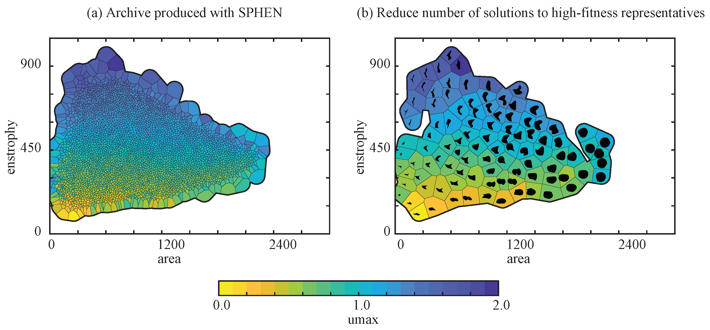
Although we used 1000 expensive simulations, we were able to evaluate, in a surrogate-assisted manner, 2,250,000 proposed solutions. After producing 1000 samples, the GP models can predict u m a x , A , and E for a diverse set of solutions. Figure 7 shows the archive produced with SPHEN.

3.3. QD Analysis Step

The user can now analyze the shapes, their features, and their correlations to fitness. Users can select high-fitness representative shape examples (Figure 7b), effectively discovering prototypes from the diverse set (see [64]). SPHEN does not have to be fully reevaluated to achieve this, except for rebuilding the archive with a smaller size. As we can already see from this archive, the lowest u m a x is reached when the area A and enstrophy E are small. However, a trade-off appears: as the larger A becomes, the higher u m a x . A positive correlation between E and u m a x is visible as well, as we expected.

3.4. Generation Step

Although we used a fixed encoding to generate the shape archive, we now have GP models that allow us to create larger archives. A new archive with 4000 solutions is trained and a VAE is trained, based on this data set. A larger data set can be created with ease, but not necessarily in this use case. The VAE will allow us to generate new solutions, interpolate between solutions, and find disentangled morphological features that help us understand the correlations between shape and flow features.
Figure 8 shows the architecture used for the convolutional VAE. The filters, with size 3 × 3 and stride 2, reduce the resolution of the input image by a factor of 2. Every convolutional layer contains more filters to hierarchically decompose (bitmaps of) the shape set into ever smaller, more low-level, morphological features. This encodes the shape into a five-dimensional space of latent variables that describe core morphological aspects of the shape set. Latent variables are comparable to principal components, except that they are non-linear. To decode the latent variables back into a shape, deconvolutions are used in the exact yet mirrored order as in the encoder.

3.5. VAE Analysis Step

The VAE’s smooth latent space offers a new morphological search space that produces only shapes with relatively low u m a x . Flow values can be predicted using GP models on the basis of latent coordinates of shapes. The VAE allows the user to vary morphological features around a selected shape.
Figure 9 shows what happens when each of the five latent variables is varied (rows). The color indicates the value of the predicted u m a x , A , and enstrophy E . The user can analyze how morphological changes influence predefined morphological features, like A or flow features. As can be seen from the figure, E and u m a x are positively related. A higher E leads to a higher u m a x , as expected.
The user might now select a shape generated by the VAE for further study. The shape selected, marked in red in Figure 9, has a higher predicted u m a x than the original shape. Now, the user chooses to run an actual simulation to validate the predicted flow features and understand why the shape has a higher u m a x . Figure 10 shows six consecutive time stamps of the flow produced with Lettuce. Vortices appear at the bottom and top sides of the view successively, shown in white and black outlines. The actual value of u m a x = 2.49 is higher than predicted. This discrepancy highlights a known challenge with simpler surrogate models when exploring novel regions of the design space, a topic we address with state-of-the-art methods in Section 2.4.2. As presented, this use case study merely shows what we can do with FDA.

3.6. Very Large Solution Sets

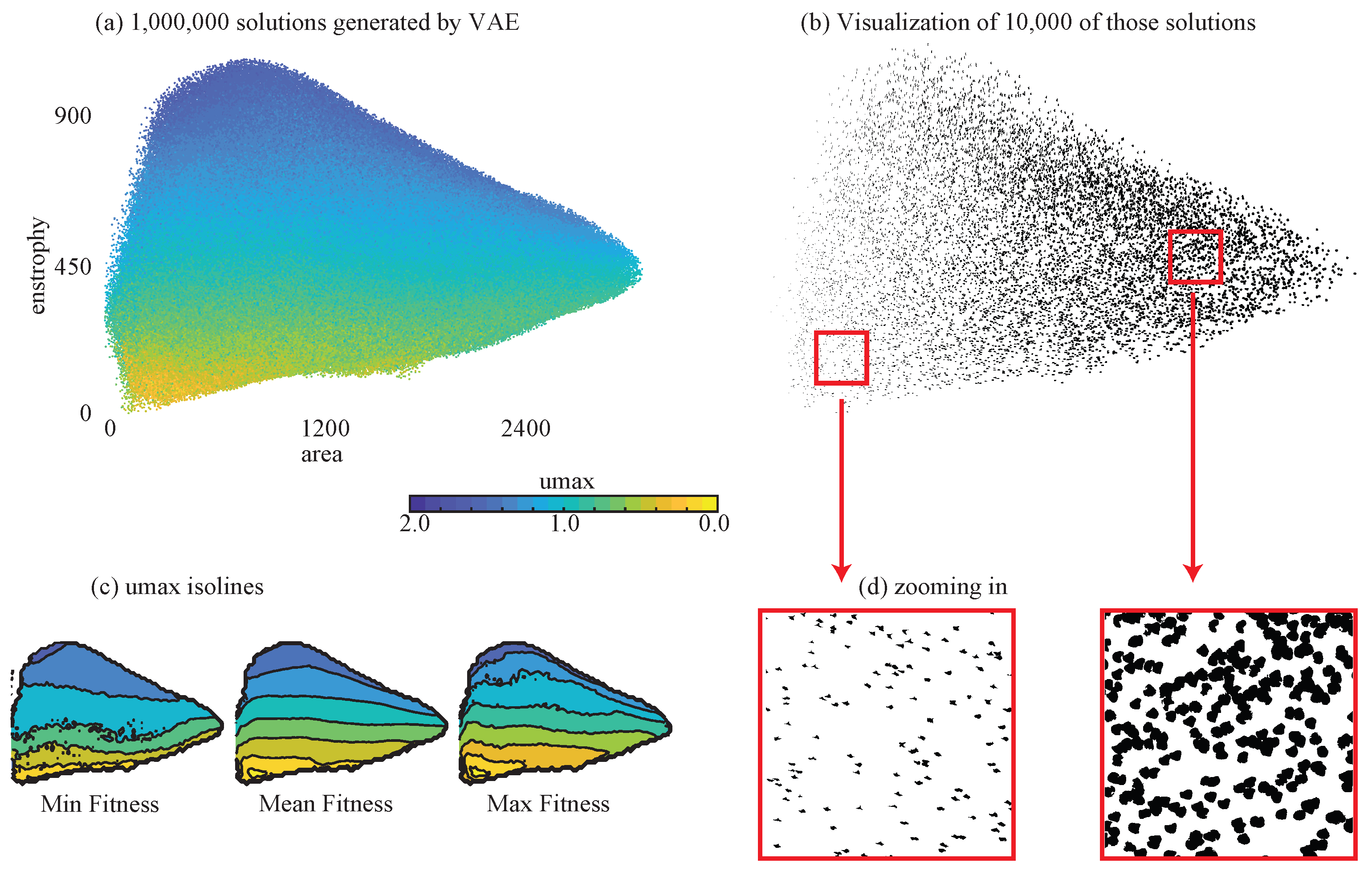
To demonstrate the scalability of FDA to its extremes, we generated 1,000,000 solutions, shown in Figure 11. It can be clearly seen that E and u m a x have an almost linear relationship (Figure 11a). However, the relationship is not purely linear, as can be seen from the minimum, mean, and maximum fitness isolines (Figure 11c).
The user can zoom in on specific regions of interest to perform a more in-depth analysis of local morphological effects (Figure 11d).
Finally, the entire example FDA system is shown in Figure 12. By using a classical encoding to bootstrap a quality–diversity algorithm, which efficiently samples a fast CFD simulation, it is possible to produce a large, diverse set of instances or shapes. A data-driven encoding is then developed to generate even more shapes, allowing the user to analyze morphological dimensions in the latent space as well as perform other in-depth analyzes. The following forms of interaction between the user and the system can be distinguished: analysis of morphological space, morphological and flow features, generating variations of shapes, selecting shapes and constraining the QD process in further iterations.

4. Discussion and Conclusions

4.1. Discussion

The ability to efficiently understand and analyze the full space of solutions and their behavior provides a powerful support tool for engineers. Possible answers to the questions asked in the introduction (Section 1) were given in this article, but we also outlined avenues for future research. We showed that direct encodings can provide us with a bootstrapping mechanism for FDA in fluid mechanics. FDA efficiency is increased using statistical models that are able to predict both the quality of solutions as well as their similarity. The models are used to guide the sampling method towards a diverse set of optima. Surrogate-assisted QD provides an efficient sampling method to find high-performing solutions based on either a manually defined encoding, for bootstrapping, or a data-driven encoding. A GPU-based LBM solver was used to determine the quality and diversity/similarity of solutions. Although other CFD solvers may also be suited, this particular LBM solver is tuned towards automated flow simulations around diverse shape sets. The results can be returned to the user, who can analyze the results efficiently and influence the sampling. This interactive analysis, supported by visualization tools that allow users to “zoom in” on regions of interest (as demonstrated in Section 3.3 and Figure 11), is a core component of the FDA framework and relies on the methods discussed in our prior work [4,11]. A latent model can be trained on the resulting set, providing a bootstrapped generator of high-quality solutions and a means to visualize and understand how morphological features are correlated to flow features.
Improvements of the presented ingredients of FDA are many, since the respective fields are developing quickly. Novel QD methods might improve the efficiency of the search even more. Examples of these methods are the integration of a faster derivative-free optimizer [99], adding differentiability when it is available [100], exchanging the sampling function [101], integrating reinforcement learning concepts (see [102]), exploring co-evolutionary approaches within QD (see [103]), or further integration of deep learning methods [104]. They are examples of how the search itself can be made more efficient and effective. The GM can be improved further by keeping track of research on disentangling the latent dimensions, making them more interpretable for humans.
New insights often lead to new focuses in the analysis of complex domains. The current development in evolutionary algorithms and machine learning enables us to more deeply understand problem domains, even when they are as expensive as fluid dynamics.

4.2. Conclusions

This paper introduced Full Domain Analysis (FDA), a methodological framework designed to synthesize evolutionary computation, machine learning, and simulation for the comprehensive exploration of complex engineering design spaces. We established the core components of FDA—(1) Encodings, (2) Search, (3) CFD, (4) Efficiency, and (5) Visualization—and reviewed the state of the art for each, integrating recent advances to demonstrate the framework’s relevance and power. The primary contribution of this work is not a single new algorithm, but the formalization of this synergistic approach and the demonstration of its utility through an illustrative 2D fluid dynamics example. We showed how surrogate-assisted quality–diversity search, combined with generative models, enables the efficient generation and interactive analysis of vast and diverse solution sets. While our illustrative example was intentionally limited in scope, we have outlined how emerging techniques like hybrid RANS-LES, diffusion models, and differentiable QD position the FDA framework to scale to more complex, real-world 3D turbulent flow problems. Ultimately, FDA provides a structured pathway for engineers to move beyond single-point optimization, fostering deeper domain understanding and accelerating the discovery of innovative and robust designs.

Author Contributions

Conceptualization, A.H. and A.G.; methodology, A.H., A.G. and D.W.; software, A.H., A.G. and D.W.; investigation, A.H. and D.W.; writing—original draft preparation, A.H. and D.W.; writing—review and editing, A.H., A.G., D.W., A.A., H.F. and D.R.; visualization, A.H.; supervision, A.A., H.F. and D.R.; project administration, D.R.; funding acquisition, A.H., A.A. and D.R. All authors have read and agreed to the published version of the manuscript.

Funding

This research was funded by the German Federal Ministry of Education and Research (BMBF) grant number 03FH012PX5. The computer hardware was supported by the Federal Ministry for Education and Research and by the Ministry for Innovation, Science, Research, and Technology of the state of North Rhine-Westphalia, grant number 13FH156IN6.

Data Availability Statement

You can find the Python code that was used as a basis for the example in the latest commit of the lettuce branch of https://github.com/alexander-hagg/sphenpy.git (accessed on 15 August 2025).

Acknowledgments

The authors would like to thank Lea Prochnau and George Khujadze for their contributions.

Conflicts of Interest

Adam Gaier was employed by the company Autodesk Research, The remaining authors declare no conflicts of interest.

Abbreviations

The following abbreviations are used in this manuscript:
FDAfull domain analysis
QDquality–diversity
MMOmultimodal optimization
MOOmultiobjective optimization
BOBayesian optimization
GPGaussian process model
FFDfree form deformation
CPPNcompositional pattern producing networks
SAOsurrogate-assisted optimization
NSGA-IInon-dominated sorting genetic algorithm
GMgenerative model
VAEvariational autoencoder
GANgenerative adversarial network
GAgenetic algorithm
NURBSnon-uniform rational b-splines
CFDcomputational fluid dynamics
SPHENsurrogate-assisted phenotypic niching
LBMlattice Boltzmann method

References

  1. Vinuesa, R.; Brunton, S.L. The potential of machine learning to enhance computational fluid dynamics. arXiv 2021, arXiv:2110.02085. [Google Scholar]
  2. Wang, Y.; Shimada, K.; Farimani, A.B. Airfoil GAN: Encoding and Synthesizing Airfoils for Aerodynamic-aware Shape Optimization. arXiv 2021, arXiv:2101.04757. [Google Scholar] [CrossRef]
  3. Gaier, A.; Asteroth, A.; Mouret, J.-B. Data-efficient design exploration through surrogate-assisted illumination. Evol. Comput. 2018, 26, 381–410. [Google Scholar] [CrossRef]
  4. Hagg, A.; Asteroth, A.; Bäck, T. Modeling user selection in quality diversity. In Proceedings of the Genetic and Evolutionary Computation Conference, Cancún, Mexico, 8–12 July 2019; pp. 116–124. [Google Scholar]
  5. Jacobs, E.N.; Ward, K.E.; Pinkerton, R.M. The Characteristics of 78 Related Airfoil Section from Tests in the Variable-Density Wind Tunnel, Report No. 460; US Government Printing Office: Washington, DC, USA, 1933. [Google Scholar]
  6. Holland, J.H. Adaptation in Natural and Artificial Systems: An Introductory Analysis with Applications to Biology, Control, and Artificial Intelligence; MIT Press: Cambridge, MA, USA, 1992. [Google Scholar]
  7. Olhofer, M.; Sendhoff, B.; Arima, T.; Sonoda, T. Optimisation of a stator blade used in a transonic compressor cascade with evolution strategies. In Evolutionary Design and Manufacture; Springer: London, UK, 2000; pp. 45–54. [Google Scholar]
  8. Lapok, P. Evolving planar mechanisms for the conceptual stage of mechanical design. Ph.D. Thesis, Edinburgh Napier University, Edinburgh, UK, 2020. [Google Scholar]
  9. Bellman, R. Dynamic programming. Science 1966, 153, 34–37. [Google Scholar] [CrossRef]
  10. Beyer, K.; Goldstein, J.; Ramakrishnan, R.; Shaft, U. When is “nearest neighbor” meaningful? In Proceedings of the International conference on database theory, Jerusalem, Israel, 10–12 January 1999; Springer: Berlin, Germany, 1999; pp. 217–235. [Google Scholar]
  11. Hagg, A. Discovering the preference hypervolume: An interactive model for real world computational co-creativity. Ph.D. Thesis, Leiden University, Leiden, The Netherlands, 2021. [Google Scholar]
  12. Nordmoen, J.; Veenstra, F.; Ellefsen, K.O.; Glette, K. MAP-Elites enables Powerful Stepping Stones and Diversity for Modular Robotics. Front. Robot. AI 2021, 8, 639173. [Google Scholar] [CrossRef]
  13. Hicks, R.M.; Murman, E.M.; Vanderplaats, G.N. An Assessment of Airfoil Design by Numerical Optimization; NASA Technical Note D-7415; National Aeronautics and Space Administration: Washington, DC, USA, 1974. [Google Scholar]
  14. Vicini, A.; Quagliarella, D. Airfoil and wing design through hybrid optimization strategies. AIAA J. 1999, 37, 634–641. [Google Scholar] [CrossRef]
  15. Sederberg, T.W.; Parry, S.R. Free-form deformation of solid geometric models. ACM SIGGRAPH Comput. Graph. 1986, 20, 151–160. [Google Scholar] [CrossRef]
  16. Sarakinos, S.S.; Amoiralis, E.; Nikolos, I.K. Exploring freeform deformation capabilities in aerodynamic shape parameterization. In Proceedings of the EUROCON 2005—The International Conference on “Computer as a Tool”, Belgrade, Serbia and Montenegro, 21–24 November 2005; IEEE: Piscataway, NJ, USA, 2005; Volume 1, pp. 535–538. [Google Scholar]
  17. Tai, K.; Wang, N.F.; Yang, Y.W. Target geometry matching problem with conflicting objectives for multiobjective topology design optimization using GA. In Proceedings of the 2008 IEEE Congress on Evolutionary Computation (IEEE World Congress on Computational Intelligence), Hong Kong, China, 1–6 June 2008; IEEE: Piscataway, NJ, USA, 2008; pp. 1873–1878. [Google Scholar]
  18. Stanley, K.O. Compositional pattern producing networks: A novel abstraction of development. Genet. Program. Evolvable Mach. 2007, 8, 131–162. [Google Scholar] [CrossRef]
  19. Gaier, A. Evolutionary Design via Indirect Encoding of Non-Uniform Rational Basis Splines. In Proceedings of the Companion Publication of the 2015 Annual Conference on Genetic and Evolutionary Computation, Madrid, Spain, 11–15 July 2015; pp. 1197–1200. [Google Scholar]
  20. Hotz, P.E. Comparing direct and developmental encoding schemes in artificial evolution: A case study in evolving lens shapes. In Proceedings of the 2004 Congress on Evolutionary Computation, Portland, OR, USA, 19–23 June 2004; IEEE: Piscataway, NJ, USA, 2004; Volume 1, pp. 752–757. [Google Scholar]
  21. Kicinger, R. Evolutionary Developmental System for Structural Design. In Proceedings of the AAAI Fall Symposium: Developmental Systems, Arlington, VA, USA, 13–15 October 2006; pp. 1–8. [Google Scholar]
  22. Clune, J.; Stanley, K.O.; Pennock, R.T.; Ofria, C. On the performance of indirect encoding across the continuum of regularity. IEEE Trans. Evol. Comput. 2011, 15, 346–367. [Google Scholar] [CrossRef]
  23. Yannou, B.; Dihlmann, M.; Cluzel, F. Indirect encoding of the genes of a closed curve for interactively create innovative car silhouettes. In Proceedings of the 10th International Design Conference-DESIGN 2008, Dubrovnik, Croatia, 19–22 May 2008; pp. 1243–1254. [Google Scholar]
  24. Clune, J.; Chen, A.; Lipson, H. Upload any object and evolve it: Injecting complex geometric patterns into CPPNs for further evolution. In Proceedings of the 2013 IEEE Congress on Evolutionary Computation, Cancun, Mexico, 20–23 June 2013; IEEE: Piscataway, NJ, USA, 2013; pp. 3395–3402. [Google Scholar]
  25. Collins, J.; Cottier, B.; Howard, D. Comparing direct and indirect representations for environment-specific robot component design. In Proceedings of the 2019 IEEE Congress on Evolutionary Computation (CEC), Wellington, New Zealand, 10–13 June 2019; IEEE: Piscataway, NJ, USA, 2019; pp. 2705–2712. [Google Scholar]
  26. Stanley, K.O.; Miikkulainen, R. Evolving neural networks through augmenting topologies. Evol. Comput. 2002, 10, 99–127. [Google Scholar] [CrossRef] [PubMed]
  27. Stanley, K.O.; D’Ambrosio, D.B.; Gauci, J. A hypercube-based encoding for evolving large-scale neural networks. Artif. Life 2009, 15, 185–212. [Google Scholar] [CrossRef]
  28. Hildebrandt, T.; Branke, J. On using surrogates with genetic programming. Evol. Comput. 2015, 23, 343–367. [Google Scholar] [CrossRef]
  29. Stork, J.; Zaefferer, M.; Bartz-Beielstein, T. Improving neuroevolution efficiency by surrogate model-based optimization with phenotypic distance kernels. In Proceedings of the International Conference on the Applications of Evolutionary Computation (Part of EvoStar), Leipzig, Germany, 24–26 April 2019; Springer: Cham, Switzerland, 2019; pp. 504–519. [Google Scholar]
  30. Stork, J.; Zaefferer, M.; Fischbach, A.; Rehbach, F.; Bartz-Beielstein, T. Surrogate-Assisted Learning of Neural Networks. arXiv 2017, arXiv:1709.07720. [Google Scholar]
  31. Hagg, A.; Zaefferer, M.; Stork, J.; Gaier, A. Prediction of neural network performance by phenotypic modeling. In Proceedings of the Genetic and Evolutionary Computation Conference Companion, Prague, Czech Republic, 13–17 July 2019; pp. 1576–1582. [Google Scholar]
  32. Regenwetter, L.; Nobari, A.H.; Ahmed, F.T. Deep generative models in engineering design: A review. Comput. Aided Des. Appl. 2024, 21, 486–510. [Google Scholar] [CrossRef]
  33. Kingma, D.P.; Welling, M. Auto-Encoding Variational Bayes. In Proceedings of the International Conference on Learning Representations (ICLR), Banff, AB, Canada, 14–16 April 2014. [Google Scholar]
  34. Rios, T.; van Stein, B.; Wollstadt, P.; Bäck, T.; Sendhoff, B.; Menzel, S. Exploiting Local Geometric Features in Vehicle Design Optimization with 3D Point Cloud Autoencoders. In Proceedings of the 2021 IEEE Congress on Evolutionary Computation (CEC), Kraków, Poland, 28 June–1 July 2021; IEEE: Piscataway, NJ, USA, 2021; pp. 514–521. [Google Scholar]
  35. Hagg, A.; Berns, S.; Asteroth, A.; Colton, S.; Bäck, T. Expressivity of parameterized and data-driven representations in quality diversity search. In Proceedings of the Genetic and Evolutionary Computation Conference, Lille, France, 10–14 July 2021; pp. 678–686. [Google Scholar]
  36. Bentley, P.J.; Lim, S.L.; Gaier, A.; Tran, L. COIL: Constrained Optimization in Learned Latent Space–Learning Representations for Valid Solutions. arXiv 2022, arXiv:2202.02163. [Google Scholar]
  37. Gómez-Bombarelli, R.; Wei, J.N.; Duvenaud, D.; Hernández-Lobato, J.M.; Sánchez-Lengeling, B.; Sheberla, D.; Aguilera-Iparraguirre, J.; Hirzel, T.D.; Adams, R.P.; Aspuru-Guzik, A. Automatic chemical design using a data-driven continuous representation of molecules. ACS Cent. Sci. 2018, 4, 268–276. [Google Scholar] [CrossRef] [PubMed]
  38. Tripp, A.; Daxberger, E.; Hernández-Lobato, J.M. Sample-efficient optimization in the latent space of deep generative models via weighted retraining. Adv. Neural Inf. Process. Syst. 2020, 33. [Google Scholar]
  39. Mathieu, E.; Rainforth, T.; Siddharth, N.; Teh, Y.W. Disentangling disentanglement in variational autoencoders. In Proceedings of the International Conference on Machine Learning, Long Beach, CA, USA, 9–15 June 2019; PMLR, 2019. pp. 4402–4412. [Google Scholar]
  40. Rios, T.; Van Stein, B.; Bäck, T.; Sendhoff, B.; Menzel, S. Point2FFD: Learning Shape Representations of Simulation-Ready 3D Models for Engineering Design Optimization. In Proceedings of the 2021 International Conference on 3D Vision (3DV), London, UK, 1–3 December 2021; IEEE: Piscataway, NJ, USA, 2021; pp. 1024–1033. [Google Scholar]
  41. Wei, Z.; Dufour, E.R.; Pelletier, C.; Fua, P.; Bauerheim, M. DiffAirfoil: An Efficient Novel Airfoil Sampler Based on Latent Space Diffusion Model for Aerodynamic Shape Optimization. In Proceedings of the AIAA AVIATION Forum, Las Vegas, NV, USA, 29 July–2 August 2024. [Google Scholar]
  42. Graves, R.; Farimani, A.B. Airfoil Diffusion: Denoising Diffusion Model For Conditional Airfoil Generation. arXiv 2024, arXiv:2408.15898. [Google Scholar]
  43. Morita, H.; Shintani, K.; Yuan, C.; Permenter, F. VehicleSDF: A 3D generative model for constrained engineering design via surrogate modeling. arXiv 2024, arXiv:2410.18986. [Google Scholar]
  44. Yang, H.; Li, S.; Zhang, Y.; Wang, J. StEik: Stabilizing the Optimization of Neural Signed Distance Representations. In Proceedings of the Advances in Neural Information Processing Systems 36, New Orleans, LA, USA, 10–16 December 2023; pp. 12745–12758. [Google Scholar]
  45. Wang, Q.; Chen, R.; Zhao, L. NeuVAS: Neural Variational Shape Editing under Sparse Geometric Constraints. ACM Trans. Graph. 2025, 44, 15:1–15:14. [Google Scholar]
  46. Zhang, Z.; Yao, W.; Li, Y.; Zhou, W.; Chen, X. Topology optimization via implicit neural representations. Comput. Methods Appl. Mech. Eng. 2023, 411, 116052. [Google Scholar] [CrossRef]
  47. Hahm, K.; Park, S.; Lee, J. Isometric Diffusion: Controllable Generation via Latent-Solution Space Isometry. In Proceedings of the International Conference on Learning Representations, Vienna Austria, 7–11 May 2024. [Google Scholar]
  48. Vafidis, N.; Thompson, D.; Mitchell, R. NashAE: Disentangled Representation Learning via Nash Equilibrium in Autoencoders. Mach. Learn. 2023, 112, 3021–3045. [Google Scholar]
  49. Scarton, L.; Hagg, A. On the Suitability of Representations for Quality Diversity Optimization of Shapes. In Proceedings of the Genetic and Evolutionary Computation Conference, Lisbon, Portugal, 15–19 July 2023; pp. 963–971. [Google Scholar]
  50. Gaier, A.; Asteroth, A.; Mouret, J.-B. Are quality diversity algorithms better at generating stepping stones than objective-based search? In Proceedings of the Genetic and Evolutionary Computation Conference Companion, Prague, Czech Republic, 13–17 July 2019; pp. 115–116. [Google Scholar]
  51. Hagg, A.; Preuss, M.; Asteroth, A.; Bäck, T. An Analysis of Phenotypic Diversity in multisolution Optimization. In Proceedings of the International Conference on Bioinspired Methods and Their Applications, Brussels, Belgium, 18–19 November 2020; Springer: Cham, Switzerland, 2020; pp. 43–55. [Google Scholar]
  52. Wang, H.; Jin, Y.; Yao, X. Diversity assessment in many-objective optimization. IEEE Trans. Cybern. 2016, 47, 1510–1522. [Google Scholar] [CrossRef]
  53. Deb, K.; Pratap, A.; Agarwal, S.; Meyarivan, T.A.M.T. A fast and elitist multiobjective genetic algorithm: NSGA-II. IEEE Trans. Evol. Comput. 2002, 6, 182–197. [Google Scholar] [CrossRef]
  54. Zitzler, E.; Laumanns, M.; Thiele, L. SPEA2: Improving the strength Pareto evolutionary algorithm. In TIK-Report 103; ETH Zurich: Zurich, Switzerland, 2001. [Google Scholar]
  55. Beume, N.; Naujoks, B.; Emmerich, M. SMS-EMOA: Multiobjective selection based on dominated hypervolume. Eur. J. Oper. Res. 2007, 181, 1653–1669. [Google Scholar] [CrossRef]
  56. Holland, J.H. Adaptation in Natural and Artificial Systems; MIT Press: Cambridge, MA, USA, 1975. [Google Scholar]
  57. DeJong, K.A. Analysis of the Behavior of a Class of Genetic Adaptive Systems. Ph.D. Thesis, University of Michigan, Ann Arbor, MI, USA, 1975. [Google Scholar]
  58. Wales, D.J.; Doye, J.P.K. Global optimization by basin-hopping and the lowest energy structures of Lennard-Jones clusters containing up to 110 atoms. J. Phys. Chem. A 1997, 101, 5111–5116. [Google Scholar] [CrossRef]
  59. Preuss, M. Improved topological niching for real-valued global optimization. In Proceedings of the European Conference on the Applications of Evolutionary Computation, Málaga, Spain, 11–13 April 2012; Springer: Berlin/Heidelberg, Germany, 2012; pp. 386–395. [Google Scholar]
  60. Pošík, P.; Huyer, W. Restarted local search algorithms for continuous black box optimization. Evol. Comput. 2012, 20, 575–607. [Google Scholar] [CrossRef]
  61. Cully, A.; Clune, J.; Tarapore, D.; Mouret, J.-B. Robots that can adapt like animals. Nature 2015, 521, 503–507. [Google Scholar] [CrossRef]
  62. Cully, A. Autonomous Skill Discovery with Quality-Diversity and Unsupervised Descriptors. In Proceedings of the Genetic and Evolutionary Computation Conference, Prague, Czech Republic, 13–17 July 2019. [Google Scholar]
  63. Gaier, A.; Asteroth, A.; Mouret, J.-B. Discovering representations for black-box optimization. In Proceedings of the 2020 Genetic and Evolutionary Computation Conference, Cancún, Mexico, 8–12 July 2020; pp. 103–111. [Google Scholar]
  64. Hagg, A.; Asteroth, A.; Bäck, T. Prototype discovery using quality-diversity. In Proceedings of the International Conference on Parallel Problem Solving from Nature, Coimbra, Portugal, 8–12 September 2018; Springer: Cham, Switzerland, 2018; pp. 500–511. [Google Scholar]
  65. Fontaine, M.C.; Nikolaidis, S. Differentiable Quality Diversity. In Proceedings of the Advances in Neural Information Processing Systems 34, Online, 6–14 December 2021; pp. 10040–10052. [Google Scholar]
  66. Boyar, A.; Kim, H.; Rodriguez, C. Latent-Consistent Acquisition for Bayesian Optimization in Learned Representations. J. Mach. Learn. Res. 2024, 25, 1–34. [Google Scholar]
  67. Lee, D.; Patel, N.; Wilson, A. Coordinate Bayesian Optimization for High-Dimensional Structured Domains. In Proceedings of the International Conference on Machine Learning, Honolulu, HI, USA, 23–29 July 2023; pp. 19234–19251. [Google Scholar]
  68. Kent, P.; Grover, A.; Abbeel, P. BOP-Elites: Bayesian Optimisation for Quality-Diversity Search. In Proceedings of the Genetic and Evolutionary Computation Conference, Cancun, Mexico, 8–12 July 2020; pp. 334–342. [Google Scholar]
  69. Alfonsi, G. Reynolds-averaged Navier-Stokes equations for turbulence modeling. Appl. Mech. Rev. 2009, 62. [Google Scholar] [CrossRef]
  70. Sagaut, P. Large Eddy Simulation for Incompressible Flows: An Introduction; Springer Science & Business Media: Berlin/Heidelberg, Germany, 2006. [Google Scholar]
  71. Löhner, R. Towards overcoming the LES crisis. Int. J. Comput. Fluid Dyn. 2019, 33, 87–97. [Google Scholar] [CrossRef]
  72. Sanderse, B.; Stinis, P.; Maulik, R.; Ahmed, S.E. Scientific machine learning for closure models in multiscale problems: A review. Comput. Fluids 2025, 291, 106186. [Google Scholar] [CrossRef]
  73. Möller, T.; Schmidt, K.; Andersson, B. Hybrid RANS-LES Performance Assessment for Industrial Turbomachinery: A Comprehensive Benchmark Study. J. Turbomach. 2024, 146, 071008. [Google Scholar]
  74. Khaled, S.; Martinez, E.; Brown, J. Deep Learning Enhanced Eddy Viscosity Models for Improved Separated Flow Predictions. Phys. Fluids 2024, 36, 045108. [Google Scholar]
  75. Ingram, D.M.; Causon, D.M.; Mingham, C.G. Developments in Cartesian cut cell methods. Math. Comput. Simul. 2003, 61, 561–572. [Google Scholar] [CrossRef]
  76. Mavriplis, D.J. Unstructured grid techniques. Annu. Rev. Fluid Mech. 1997, 29, 473–514. [Google Scholar] [CrossRef]
  77. Balan, A.; Park, M.A.; Wood, S.L.; Anderson, W.K.; Rangarajan, A.; Sanjaya, D.P.; May, G. A review and comparison of error estimators for anisotropic mesh adaptation for flow simulations. Comput. Fluids 2022, 234, 105259. [Google Scholar] [CrossRef]
  78. Jin, Y. Surrogate-assisted evolutionary computation: Recent advances and future challenges. Swarm Evol. Comput. 2011, 1, 61–70. [Google Scholar] [CrossRef]
  79. Wessing, S. Two-Stage Methods for Multimodal Optimization. Ph.D. Thesis, Technische Universität Dortmund, Dortmund, Germany, 2015. [Google Scholar]
  80. Hagg, A.; Wilde, D.; Asteroth, A.; Bäck, T. Designing Air Flow with Surrogate-assisted Phenotypic Niching. In Proceedings of the International Conference on Parallel Problem Solving from Nature, Leiden, The Netherlands, 5–9 September 2020; Springer: Cham, Switzerland, 2020; pp. 140–153. [Google Scholar]
  81. Burgess, C.P.; Higgins, I.; Pal, A.; Matthey, L.; Watters, N.; Desjardins, G.; Lerchner, A. Understanding Disentangling in Beta-VAE. In Proceedings of the NIPS Workshop on Learning Disentangled Representations, Long Beach, CA, USA, 8–9 December 2017. [Google Scholar]
  82. Antonova, R.; Rai, A.; Li, T.; Kragic, D. Bayesian optimization in variational latent spaces with dynamic compression. In Proceedings of the Conference on Robot Learning, Virtual Event, 16–18 November 2020; PMLR, 2020. pp. 456–465. [Google Scholar]
  83. Wu, H.; Liu, X.; An, W.; Chen, S.; Lyu, H. A deep learning approach for efficiently and accurately evaluating the flow field of supercritical airfoils. Comput. Fluids 2020, 198, 104393. [Google Scholar] [CrossRef]
  84. Chen, L.-W.; Cakal, B.A.; Hu, X.; Thuerey, N. Numerical investigation of minimum drag profiles in laminar flow using deep learning surrogates. J. Fluid Mech. 2021, 919, A34. [Google Scholar] [CrossRef]
  85. Lye, K.O.; Mishra, S.; Ray, D. Deep learning observables in computational fluid dynamics. J. Comput. Phys. 2020, 410, 109339. [Google Scholar] [CrossRef]
  86. Lino, S.; Fotiadis, S.; Bharath, A.A.; Cantwell, C.D. Current and emerging deep-learning methods for the simulation of fluid dynamics. Proc. R. Soc. A Math. Phys. Eng. Sci. 2023, 479, 20230058. [Google Scholar] [CrossRef]
  87. Sun, L.; Gao, H.; Pan, S.; Wang, J.-X. Surrogate modeling for fluid flows based on physics-constrained deep learning without simulation data. Comput. Methods Appl. Mech. Eng. 2020, 361, 112732. [Google Scholar] [CrossRef]
  88. Ibrahim, S.M.; Najmi, M.I. Computational Fluid Dynamics (CFD) Optimization in Smart Factories: AI-Based Predictive Modelling. J. Technol. Inform. Eng. 2025, 4, 56–74. [Google Scholar] [CrossRef]
  89. Forrester, A.I.J.; Sóbester, A.; Keane, A.J. Multi-fidelity optimization via surrogate modelling. Proc. R. Soc. A Math. Phys. Eng. Sci. 2007, 463, 3251–3269. [Google Scholar] [CrossRef]
  90. Koziel, S.; Cheng, Q.S.; Bandler, J.W. Space mapping. IEEE Microw. Mag. 2008, 9, 105–122. [Google Scholar] [CrossRef]
  91. Li, F.; Wang, S.; Kumar, V. Multi-Fidelity POD-Enhanced Neural Surrogates for Parametric Navier-Stokes Equations. Comput. Methods Appl. Mech. Eng. 2024, 418, 116578. [Google Scholar]
  92. Zhang, L.; Adams, R.; Taylor, M. Multi-Fidelity Uncertainty Quantification: Methods, Applications, and Future Directions. Annu. Rev. Fluid Mech. 2024, 56, 285–312. [Google Scholar]
  93. Li, R.; Huang, Z.; Wang, W. PG-Diff: A Physics-Informed Self-Guided Diffusion Model for High-Fidelity Simulations. In Proceedings of the International Conference on Learning Representations, Singapore, 24–28 April 2025. [Google Scholar]
  94. Du, P.; Parikh, M.H.; Fan, X.; Liu, X.Y.; Wang, J.X. Conditional neural field latent diffusion model for generating spatiotemporal turbulence. Nat. Commun. 2024, 15, 10416. [Google Scholar] [CrossRef]
  95. NEN 8100; Wind Comfort and Wind Danger in the Built Environment. NEN: Delft, The Netherlands, 2006.
  96. Bedrunka, M.C.; Wilde, D.; Kliemank, M.; Reith, D.; Foysi, H.; Krämer, A. Lettuce: PyTorch-based Lattice Boltzmann Framework. In Proceedings of the International Conference on High Performance Computing, Frankfurt, Germany, 14–18 June 2021; Springer: Cham, Switzerland, 2021; pp. 40–55. [Google Scholar]
  97. Sobol’, I.M. On the distribution of points in a cube and the approximate evaluation of integrals. Zh. Vychisl. Mat. Mat. Fiz. 1967, 7, 784–802. [Google Scholar] [CrossRef]
  98. Rasmussen, C.E.; Nickisch, H. Gaussian processes for machine learning (GPML) toolbox. J. Mach. Learn. Res. 2010, 11, 3011–3015. [Google Scholar]
  99. Fontaine, M.C.; Togelius, J.; Nikolaidis, S.; Hoover, A.K. Covariance matrix adaptation for the rapid illumination of behavior space. In Proceedings of the 2020 Genetic and Evolutionary Computation Conference, Cancún, Mexico, 8–12 July 2020; pp. 94–102. [Google Scholar]
  100. Fontaine, M.; Nikolaidis, S. Differentiable Quality Diversity. Adv. Neural Inf. Process. Syst. 2021, 34, 10040–10052. [Google Scholar]
  101. Kent, P.; Branke, J. Bop-elites, a bayesian optimisation algorithm for quality-diversity search. arXiv 2020, arXiv:2005.04320. [Google Scholar]
  102. Grillotti, L.; Faldor, M.; León, B.G.; Cully, A. Quality–Diversity Actor–Critic Learning High–Performing and Diverse Behaviors via Value and Successor Features Critics. arXiv 2024, arXiv:2403.09930. [Google Scholar]
  103. Timothée, A.; Syrkis, N.; Elhosni, M.; Turati, F.; Legendre, F.; Jaquier, A.; Risi, S. Adversarial Coevolutionary Illumination with Generational Adversarial MAP-Elites. arXiv 2024, arXiv:2402.11951. [Google Scholar]
  104. Zhang, Y.; Fontaine, M.C.; Hoover, A.K.; Nikolaidis, S. Deep Surrogate Assisted MAP-Elites for Automated Hearthstone Deckbuilding. arXiv 2021, arXiv:2112.12782. [Google Scholar]
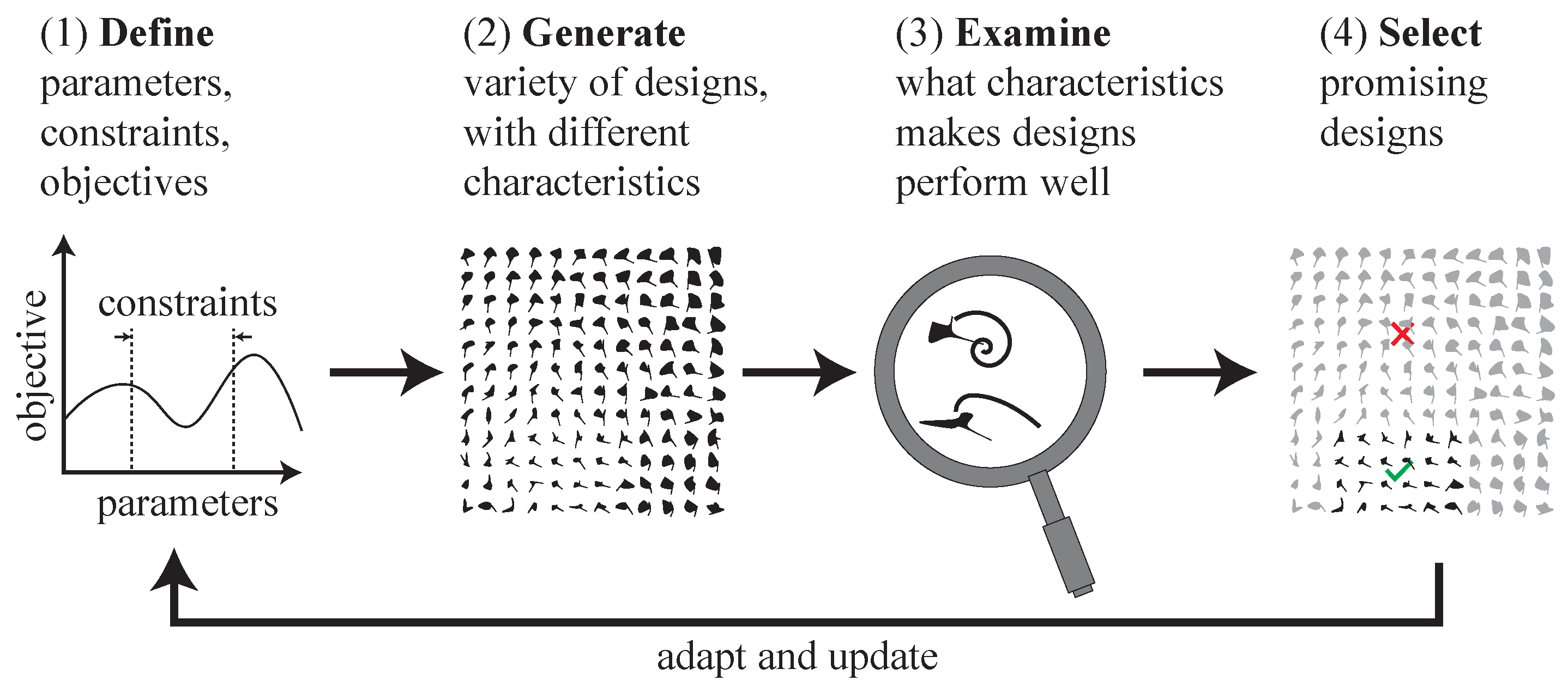
Figure 1. User process perspective on FDA. After the user defines the domain through available initial parameters, constraints, and objectives, the prior (1), a large variety of designs is automatically generated (2). The user examines what makes designs perform well (3). They then select promising design regions (green checkmark), which allows FDA to update the initial domain definition (4). The next iteration of the FDA process zooms in on the user’s region of interest.
Make 07 00086 g001
Figure 2. While search and optimization take place in what we call the parameter space X , through the encoding’s expression and its in situ simulation, only a part of the solution space S can be reached, the reachable manifold R . This manifold might include invalid solutions (necessitating constraints on the parameter space). The goal is to maximize R w.r.t. the valid subspace V .
Make 07 00086 g002
Figure 3. Three main categories of shape encodings to produce solutions in S . Direct, parameterized encodings use a manually defined decoder that determines spline shapes. Indirect encodings search the shapes indirectly by performing a search on the functional structure of the decoder. The decoder determines which pixel or voxel in a discretized solution is filled. Data-driven latent-generative approaches use pre-trained generative models that compress a set of prior examples to a low-dimensional latent space, which serves as a search space X .
Make 07 00086 g003
Figure 4. Heterogeneous fitness landscapes often contain clusters of varying sizes, making the definition of “local optimum” in terms of a threshold distance value ϵ indeterminable. ϵ 1 and ϵ 2 vary.
Make 07 00086 g004
Figure 5. Multisolution optimization. Multiobjective optimization (a) finds a Pareto front of trade-off solutions. Solutions are added to the front if they dominate neighboring solutions in at least one objective. In multimodal optimization (b), solutions are selected through local competition in the parameter space. Quality–diversity (c) searches in parameter space, but local competition takes place in a low-dimensional archive defined by characteristics of their morphology or behavior.
Make 07 00086 g005
Figure 6. Encoding of 2D shapes: eight control points’ polar coordinates.
Make 07 00086 g006
Figure 7. After efficiently training surrogate models for the features (area and enstrophy/turbulence) and fitness of a diverse solution set, we can easily produce an archive of 4000 solutions (a) and reduce the solution set size to its best 100 representatives (b).
Make 07 00086 g007
Figure 8. Architecture of the convolutional VAE generative model.
Make 07 00086 g008
Figure 9. The three features are shown for a shape and its variants when varying five latent dimensions in a VAE model. Please note that the color schemes used for E and u m a x are flipped. The red box marks a similar shape with a higher u m a x than the originally selected one (center column). The overall positive correlation between enstrophy E and u m a x is visible in the color patterns across the generated shapes.
Make 07 00086 g009
Figure 10. Flow around selected shape. The top row shows the appearance of a strong vortex (white outline) caused by the bottom of the shape. The bottom row shows a weak vortex (black outline) caused by the top of the shape, appearing after the strong vortex.
Make 07 00086 g010
Figure 11. 1,000,000 solutions generated by VAE (a), subselection of 10,000 shapes (b), isolines of min, mean and max fitness (c), and zoomed in shape regions (d).
Make 07 00086 g011
Figure 12. FDA implementation example. First, the QD process is bootstrapped with a predefined spline encoding. Using surrogate models to assist with predicting and sampling examples based on their quality and diversity, QD produces an archive of the solution space that is presented to the user. A data-driven encoding can be trained based on the shapes from the QD archive. Using this encoding and the archive, the user can analyze the solution space. They can then zoom in on a region of that space, analyze data-driven morphological features, their correlation to flow features and interact with the system. The data-driven encoding both compresses the search space and can serve for further investigation and search and provide new diversity metrics to be fed back into the QD process.
Make 07 00086 g012
Table 1. Overview of encoding types and requirements. The symbols denote the following: (+) Positive/Advantageous, (+/−) Neutral/Context-Dependent, (−) Negative/Hard. A significant challenge requiring considerable effort.
DirectIndirectLatent
Reachability− Limited, hand-coded+ High+/− Can be limited by training data
Validity+ Controllable− Hard to constrain− Hard to constrain
Searchability+ Low-dimensional− No gradients+ Potentially lower dimensionality
Predictability+ Well-understood+/− Context-dependent+/− Possible, active research
Understanding+ Interpretable− Black-box nature− Needs disentangling
Prior Knowledge+/− Manual design+/− Via structure+ Data-driven by design
Table 2. Overview of multisolution paradigms and their requirements.
ParadigmCoverageDiversityApplicability
MOONo, Pareto frontobjectives, lowcompeting features
MMOYes (par.)parameters, higher fitnessno features
QDYesfeatures, higher diversitybehavioral features
Disclaimer/Publisher’s Note: The statements, opinions and data contained in all publications are solely those of the individual author(s) and contributor(s) and not of MDPI and/or the editor(s). MDPI and/or the editor(s) disclaim responsibility for any injury to people or property resulting from any ideas, methods, instructions or products referred to in the content.