Article

A Comparison Between Unimodal and Multimodal Segmentation Models for Deep Brain Structures from T1- and T2-Weighted MRI

1
Department of Electrical and Information Engineering, Polytechnic University of Bari, Via Giuseppe Re David 4, 70126 Bari, Italy
2
Masmec Biomed SpA, Via delle Violette 14, 70026 Bari, Italy
*
Authors to whom correspondence should be addressed.
Mach. Learn. Knowl. Extr. 2025, 7(3), 84; https://doi.org/10.3390/make7030084
Submission received: 16 June 2025 / Revised: 10 July 2025 / Accepted: 8 August 2025 / Published: 13 August 2025
(This article belongs to the Special Issue Deep Learning in Image Analysis and Pattern Recognition, 2nd Edition)

Abstract

Accurate segmentation of deep brain structures is critical for preoperative planning in such neurosurgical procedures as Deep Brain Stimulation (DBS). Previous research has showcased successful pipelines for segmentation from T1-weighted (T1w) Magnetic Resonance Imaging (MRI) data. Nevertheless, the role of T2-weighted (T2w) MRI data has been underexploited so far. This study proposes and evaluates a fully automated deep learning pipeline based on nnU-Net for the segmentation of eight clinically relevant deep brain structures. A heterogeneous dataset has been prepared by gathering 325 paired T1w and T2w MRI scans from eight publicly available sources, which have been annotated by means of an atlas-based registration approach. Three 3D nnU-Net models—unimodal T1w, unimodal T2w, and multimodal (encompassing both T1w and T2w)—have been trained and compared by using 5-fold cross-validation and a separate test set. The outcomes prove that the multimodal model consistently outperforms the T2w unimodal model and achieves comparable performance with the T1w unimodal model. On our dataset, all proposed models significantly exceed the performance of the state-of-the-art DBSegment tool. These findings underscore the value of multimodal MRI in enhancing deep brain segmentation and offer a robust framework for accurate delineation of subcortical targets in both research and clinical settings.

1. Introduction

The human thalamus, which is located centrally in the brain, copes with the processing and transmission of motor and sensory signals between the cerebral cortex and various subcortical regions [1]. It is possible to identify different neuronal clusters, each of which can be subdivided into sub-nuclei, such as the subthalamic nucleus (STN), which is a biconvex glutamatergic structure located within the subcortex [2]. These sub-nuclei have been associated with such diseases as epilepsy [3] and, mainly, Parkinson’s disease (PD) [4,5,6,7,8].
The symptoms of such pathologies can be treated with Deep Brain Stimulation (DBS) [6], a neurosurgical procedure performed in the event of no response to drug treatment [2,9]. Since its success is derived from the electrode placement in subcortical regions [7], the STN may be accurately identified by means of microelectrode recording. However, it potentially increases both the surgical operation time [10] and the risk for the patient due to infection or bleeding [6]. Therefore, an alternative method for segmenting the STN is crucial for both optimizing the intervention by limiting the area of interest [1] and ensuring the patient’s safety by minimizing side effects [6].
Magnetic Resonance Imaging (MRI) offers the possibility to visualize the STN and its boundaries in advance [8]. Hence, MRI has been a valid tool to support preoperative planning for DBS by the automatic segmentation of the STN and its surrounding structures. Nonetheless, this annotation mode demands both extreme domain knowledge and a high amount of time for its accomplishment [4], which is higher and higher for each new segmentation [10]. Moreover, such identification of the STN is complicated by its variability in shape and orientation, together with its small size [6].
Standardized anatomical atlases have been created to help visualize and identify deep brain structures consistently and efficiently. Baniasadi et al. [3] have proposed an automatic approach for the automatic segmentation of 30 selected brain structures, combining information obtained from three anatomic atlases for the brain: CIT168 [11] (California Institute of Technology), DISTAL [12] (DBS Intrinsic Template Atlas), and THOMAS [13] (THalamus Optimized Multi Atlas Segmentation). Among them, DISTAL has proven particularly valuable for DBS planning, offering high-resolution, multimodal segmentations of key subcortical targets within the MNI (Montreal Neurological Institute-Hospital) space [14].
Integrated into the Lead-DBS [15,16,17] platform, DISTAL facilitates accurate localization of structures such as the red nucleus (RN), globus pallidus externus (GPe), globus pallidus internus (GPi), and STN, which are crucial for neurosurgical targeting in the treatment of movement disorders. By offering anatomically consistent boundaries, the atlas reduces inter-operator variability and facilitates both research and clinical applications, leading to more accurate electrode placement and better patient outcomes.
One challenge in this context is the limited visibility of deep brain nuclei in T1-weighted (T1w) images, especially compared to surrounding regions such as the thalamus, due to iron deposition [18]. T2-weighted (T2w) images offer higher contrast in these areas and can be integrated into the segmentation framework to improve performance [19]. However, T2w images suffer from poor contrast in the cortical regions [18], which limits their standalone effectiveness.
Therefore, the development of automated segmentation methods becomes essential, particularly for cases where structures like the STN are not clearly visible. These methods can greatly assist in neurosurgical planning and targeting [1], and they may be grounded on deep learning (DL) frameworks [20,21,22] such as nnU-Net [23,24], whose encoder–decoder architecture allows for automatically learning features from the image by exploiting ground-truth masks, which can either be manually annotated or generated through atlas-based approaches. Remarkably, Baniasadi and colleagues [3] exploited nnU-Net for the segmentation of 30 deep brain structures; however, their approach was based only on T1w images and, consequently, their proposed tool, DBSegment, cannot be applied to T2w images. Furthermore, by using only one image modality, they did not assess the eventual advantage of processing multimodal MRI data.
A group from Karolinska Institutet and Stockholm University proposed a DL approach, based on nnU-Net, for segmenting the STN, RN, and substantia nigra (SN) [19]. They leveraged multimodal data, involving Quantitative Susceptibility Mapping (QSM), T1w, FLAIR, and R 2 * images. They trained models on 40 manually annotated subjects, finding that the best combination was QSM and FLAIR. The models were then applied to an independent 3-year longitudinal dataset of 175 healthy individuals to study age-related iron accumulation.
Solomon et al. [25] introduced GP-Net, a DL approach that leverages attention-gated networks to segment GPe and GPi from 7T T2w scans. The model was trained using manual annotations from 58 subjects and validated on 43 held-out cases. The overall cohort of 101 subjects included 24 healthy controls and 77 patients with movement disorders.
Beliveau and colleagues [26] evaluated five 3D CNN architectures (U-Net, V-Net, U-Net++, FC-Dense Net, and Dilated FC-Dense Net) for the automated segmentation of iron-rich deep brain nuclei (SN, STN, RN, and dentate nucleus) from susceptibility-weighted imaging (SWI). The model was trained on a dataset of 30 SWI images from healthy controls and externally validated on 17 SWI images from the Forrest Gump dataset [27].
While these studies show good performance on their designated validation datasets, they also have some limitations: they used small datasets, which may not be enough to ensure adequate generalization capabilities with respect to patient conditions or scanning protocols; these methods rely on 7T MRI scans or on QSM or SWI image modalities, which are not routinely used in clinical practice; and these works did not focus on all of the structures of DISTAL.
In this work, we propose a fully automated workflow for the segmentation of the deep brain structures included in DISTAL (i.e., GPe-L, GPe-R, GPi-L, GPi-R, RN-L, RN-R, STN-L, STN-R), through DL. After a careful stage of data collection and preparation, three different models, two unimodal (UM) and one multimodal (MM), were trained with the nnU-Net framework: UM T1w, UM T2w, and MM. These models were thoroughly compared with 5-fold cross-validation and on a designated test set, offering precise details about the evaluation of such models and whether a multimodal approach should be more suitable for segmentation in this case.
Our main contributions are fourfold and can be summarized as follows:
  • A heterogeneous dataset comprising 325 T1w and 325 T2w MRI scans was built by integrating data from eight public sources, enabling robust training and evaluation.
  • An end-to-end multimodal framework was developed for labeling MR images, preprocessing data, and training and evaluating deep learning models for the segmentation of deep brain structures in neurosurgical settings.
  • A detailed comparison between unimodal and multimodal models was conducted, highlighting the benefits and limitations of each approach.
  • The developed T1w-based models were benchmarked against the state-of-the-art DBSegment tool, demonstrating clear improvements across all metrics.
The remainder of this article is structured as follows: Section 2 describes the materials (i.e., the publicly available dataset from which we gathered images, together with data annotation and preparation for segmentation) and methods (i.e., the training, evaluation, and statistical comparison of the presented DL models). The results are shown and discussed in Section 3 and Section 4, respectively. Ultimately, conclusions about the conducted study and suggestions for future research are reported in Section 5.

2. Materials and Methods

The general workflow employed for this study is portrayed in Figure 1. It encompasses data acquisition and annotation through atlas-based segmentation, followed by a preprocessing phase involving defacing, resampling, and reorientation. The resulting images were then used to train and evaluate three nnU-Net models—UM T1w, UM T2w, and MM—supporting the automated segmentation of deep brain structures for neurosurgical planning.

2.1. Dataset Collection

The models used in the proposed framework have been trained, validated, and tested by means of data from 8 public datasets:
  • HCP (Human Connectome Project) [28], which includes diffusion and anatomical neuroimaging data openly available to the scientific community for examination and exploration.
  • OASIS3 (Open Access Series of Imaging Studies 3) [29], which is a retrospective compilation of data for 1378 participants with 2842 MRI sessions (encompassing T1w, T2w, and FLAIR, among others).
  • ADNI (Alzheimer’s Disease Neuroimaging Initiative) [30], which is a longitudinal study started in 2004 that continuously expanded its data collection through multiple phases, contributing significantly to Alzheimer’s research. The ADNI dataset includes a variety of data types, such as clinical, biofluid, genetic, and imaging data, all of which are accessible to authorized researchers through the LONI Image and Data Archive (IDA). The latest phase of the study, ADNI4, is used in our final dataset and includes both T1w and T2w MRI scans.
  • IXI (Information eXchange from Images) [31], which is a project that collected nearly 600 MR images from healthy subjects. The MR image acquisition protocols encompass T1w, T2w, and PD (Proton Density)-weighted images.
  • UNC (University of North Carolina) [32], which includes paired T1-weighted and T2-weighted MRI scans acquired at both 3T and 7T from 10 healthy volunteers. The images were collected as part of a brain imaging study conducted by the University of North Carolina.
  • THP (Traveling Human Phantom) [33]: This OpenNeuro dataset (accession number ds000206) was collected as part of a multi-site neuroimaging reliability study. It contains repeated multimodal MRI scans acquired from five healthy individuals across eight different imaging centers.
  • NLA (Neural Correlates of Lidocaine Analgesic) [34]: This OpenNeuro dataset (accession number ds005088) includes T1w and T2w MRI scans acquired at 3T from 27 adults who participated in a single-arm, open-label study investigating the neural effects of lidocaine as an analgesic.
  • neuroCOVID [35]: This OpenNeuro dataset (accession number ds005364) includes MRI data from a total of 100 participants who underwent T1w and T2w scans as part of an evaluation of the neurological effects of COVID-19.
The cross-validation set (CVAL) was built with 260 subjects from HCP, OASIS3, ADNI4, IXI, UNC, THP, NLA, and neuroCOVID, whereas the test set (TEST) was realized with 65 subjects from OASIS3, ADNI4, IXI, and neuroCOVID.
We collected a heterogeneous dataset, including images acquired from various scanners, using different acquisition protocols and intensity ranges. The data included both healthy individuals and patients with cognitive decline (from mild conditions to Alzheimer’s disease) and respiratory disorders (infectious diseases also including COVID-19) across a wide range of ages. To prevent overfitting to any single dataset, a similar number of subjects was selected from each dataset. All of the datasets, except for THP and UNC, contain only one scan for each modality from each subject. Detailed information about the training and test data is provided in Table 1.

2.2. Data Annotation

The segmentation maps of the structures were derived from the probabilistic DISTAL [12]. All labels were generated in MNI space (ICBM 2009b Nonlinear Asymmetric) [36]. DISTAL [12] was specifically developed for Lead-DBS and is precisely aligned to the MNI space. DISTAL is the result of the fusion of neuroimaging, neurobiology, and computational neuroscience expertise, by integrating multimodal data including MRI, histology, and structural connectivity to ensure high anatomical fidelity. Unlike other neuroanatomical atlases, DISTAL was explicitly built for DBS applications, addressing the issue of mismatch between the atlas and template space that can arise when millimeter-level accuracy is essential [15].
A label file containing the segmentations of the 8 selected brain structures, together with a brain mask designed to enhance network performance by guiding it to the brain region, was generated. Each structure was first resampled to the MNI space, using the ANTsPy library (v. 0.5.4), and then binarized by applying a threshold of 0.5. The brain mask was also obtained in MNI space with Lead-DBS. Then, it was combined with the segmentation labels of the other structures into a single file using 3D Slicer [37]. Here, a unique index was assigned to each structure for consistent identification. The label names and their associated indices are shown in Table 2.
The T1w and T2w images of each subject were annotated using the generated label file, following an atlas-based method similar to those described in previous pipelines [3,38]. The GPe, GPi, RN, and STN were directly segmented in the native space of each subject through the Lead-DBS workflow [16], excluding electrode localization and reconstruction steps. Initially, a bias-field correction was applied to the T1w and T2w images using the N4 algorithm [39]. After correction, the T2w images were co-registered to the T1w images using ANTs [40] through a two-step linear registration process (rigid followed by affine) to compute the corresponding transformation matrix. The images were then normalized to the MNI 2009b template space using the Symmetric Normalization (SyN) algorithm from ANTs [40]; this step generated a nonlinear deformation field representing the transformation from the subject’s native space to the MNI space, saved as an NIfTI transformation file. Using the computed transformations, the segmentation labels were warped from the MNI space to each subject’s native image space, resulting in subject-specific segmentations of the targeted brain structures. All registrations were visually inspected to ensure accuracy and consistency. Only images that passed this quality control step were included in the dataset. In cases of a registration failure producing visibly incorrect segmentations, the corresponding subjects were excluded to prevent potential misguidance during network training.

2.3. Data Preparation

Facial information haws removed using PyDeface (v. 2.0.2) [41] to ensure consistency and anonymization across the dataset; defacing was applied only to MRI scans where facial structures had not yet been removed by the original creators of the dataset.
In this study, all MR images and corresponding ground-truth masks were isotropically resampled to a voxel spacing of 1 mm3, resized to dimensions of 256 × 256 × 256, and reoriented to the left–posterior–inferior (LPI) coordinate system. After preprocessing, the dataset was organized into the folder structure required by the nnU-Net framework [23]. This format was inspired by the data organization used in the Medical Segmentation Decathlon (MSD). Each MSD-like dataset has three components: raw images, the corresponding ground-truth segmentation maps, and a JSON file containing appropriate metadata.
Three separate datasets, one for each of the implemented models, were prepared: UM T1w, UM T2w, and MM (incorporating both T1w and T2w). For the unimodal models, the input consisted of the original T1w or T2w images, respectively, together with their corresponding segmentation maps. For the multimodal model, the dataset included co-registered T1w and T2w images, accompanied by a single set of segmentation maps consistent across both modalities, obtained during the labeling process in the co-registered space.
All default nnU-Net preprocessing steps were applied prior to training, including automatic cropping around the foreground to reduce memory usage, intensity normalization (z-score with mean = 0 and standard deviation = 1) for MRI data, and resampling the images to voxel spacing and dimensions that are the median of the training data. Data augmentation was employed during training. The following transformations were included in the data augmentation: rotations, scaling, Gaussian noise, Gaussian blur, brightness, contrast, simulation of low resolution, gamma correction, and mirroring.

2.4. Models’ Architecture and Training

Three 3D full-resolution models were trained with the nnU-Net framework, which implements a U-Net architecture with an encoder–decoder structure and skip connections. The automatic configuration of nnU-Net is driven by a combination of fixed parameters, rule-based parameters, and empirical parameters derived from the specific dataset. To assess the generalization capability of each model, nnU-Net automatically performed a 5-fold cross-validation on a dataset of 260 MR images (CVAL), with each fold comprising 208 training and 52 validation scans.
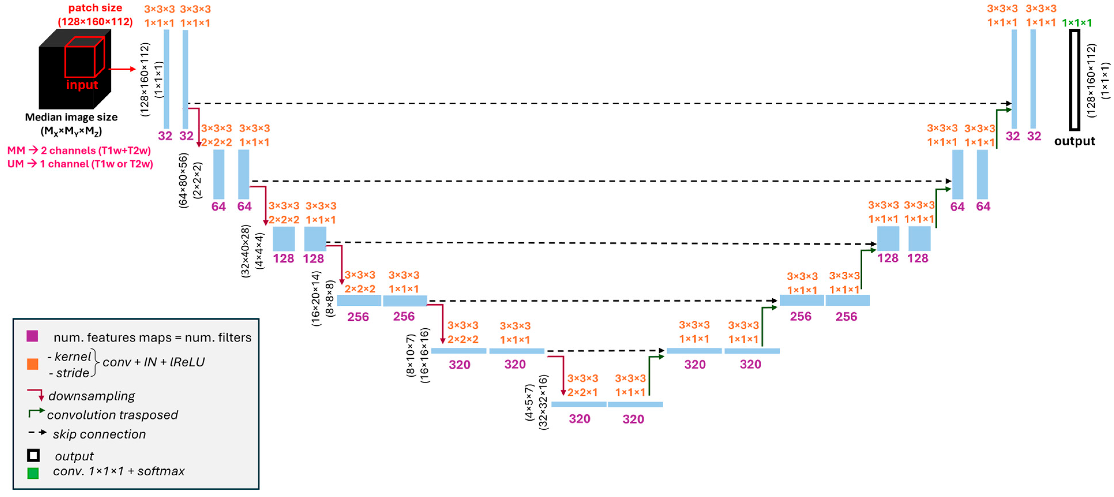
All models were trained using a batch size of 2 and a patch size of 128 × 128 × 112. The network architecture was composed of 6 stages, with the depth of the feature maps increasing from 32 to 320. Each stage included two 3D convolutional layers with kernel sizes of 3 × 3 × 3, followed by instance normalization and the Leaky ReLU activation. Downsampling was performed with 3D convolutional layers with strides of [2, 2, 2] after each level, except for the last stage, which used [2, 2, 1]. Upsampling was carried out with 3D transposed convolutional layers that compensated for downsample levels introduced in the symmetrical part of the encoder. A detailed representation of the employed architecture is portrayed in Figure 2.
The networks were trained for a fixed number of 1000 epochs, with each epoch comprising 250 training iterations. Stochastic gradient descent with Nesterov momentum (μ = 0.99) was used as an optimizer. The multimodal variant shares the same architectural design as the unimodal models, except for the input layer, which has been adapted to accept two channels corresponding to the T1w and T2w modalities.
Overall, five different networks (five folds) were trained for each of the three configurations (UM T1w, UM T2w, and MM). The performance of the network for each fold was evaluated on the 52 validation scans. Finally, an ensemble with all of the networks from the folds was constructed. The final predictions obtained by this ensemble were evaluated on 65 new MR images (TEST), which were completely independent from the CVAL.
The models were trained and validated using Python (v. 3.10.16), including the libraries nnunetv2 (v. 2.6.0), torch (v. 2.6.0+cu118), and torchvision (v. 0.21.0+cu118).

2.5. Evaluation Metrics

The network performances were evaluated using the Dice coefficient (Dice), Relative Volume Difference (RVD), Average Symmetric Surface Distance (ASSD), and Intersection over Union (IoU). These metrics were computed by comparing the segmentations generated by the network with those obtained by the registration-based method (gold standard). All of the metrics were calculated separately for each structure.
Dice and IoU are defined by Equation (1) and Equation (2), respectively. These quality measures are based on the volumetric overlap between predicted and ground-truth masks. RVD, based on the Relative Volume Difference between predicted and ground-truth masks, is defined by Equation (3). In all of the definitions, P and G indicate the volume predicted by the network and the ground-truth volume, respectively.
ASSD is a metric based on the external surface distances. To define these distances, we define a metric space ( X ,   d ) , where X is a 3D Euclidean space and d is the Euclidean distance over the space. We can define S P ,   S G X as the external surfaces of the predicted and ground-truth volumes, respectively [42]. Then, ASSD can be calculated as defined in Equation (4).
Dice   P , G = 2 · P G P + G
IoU   P , G = P G P G
RVD   P , G = P G G
ASSD S P ,   S G = 1 S P + S G   s P   S P d s P ,   S G + s G   S G d s G ,   S P

2.6. Statistical Evaluation

The models were statistically compared by means of the Wilcoxon signed-rank test with the two-sided option for each metric and on each segmented structure, allowing for the detection of statistically significant differences in both directions. Multiple hypothesis testing was considered for the analyzed deep brain structures, by employing corrected p-values with the Benjamini–Hochberg [43] method for false discovery rate.
All of the performance evaluations and their statistical analyses were conducted using Python (v. 3.12.3), including the libraries scipy (v. 1.14.1), matplotlib (v. 3.10.0), MedPy (v. 0.5.2), numpy (v. 1.26.4), pandas (v. 2.2.3), and seaborn (v. 0.13.2).

3. Results

3.1. Cross-Validation Results

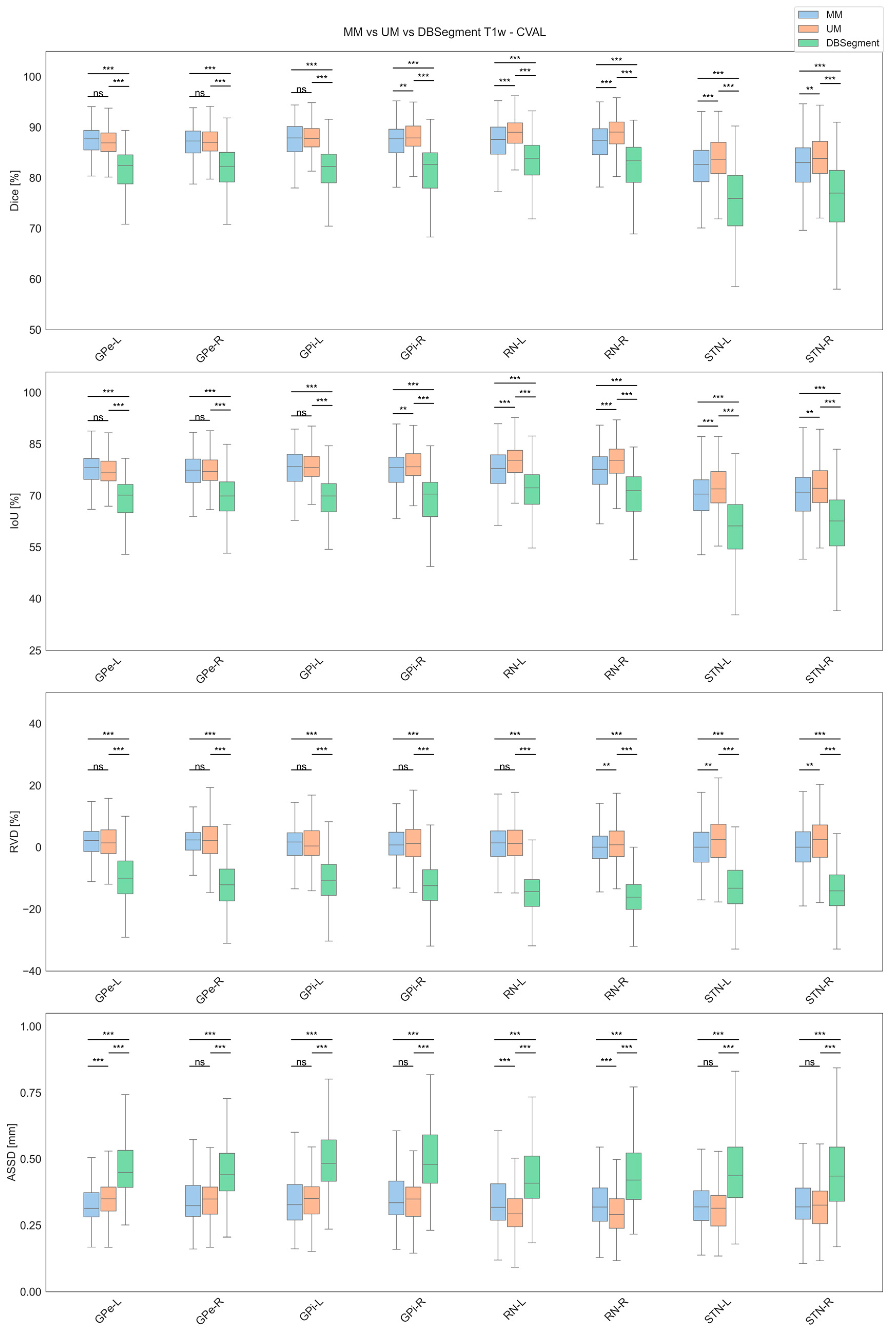
The boxplots of the T1w CVAL comparing all of the considered structures (GPe-L, GPe-R, GPi-L, GPi-R, RN-L, RN-R, STN-L, and STN-R), using Dice, IoU, RVD, and ASSD, are pictorially depicted in Figure 3. These results are complemented by the means and standard deviations reported in Table 3. Overall, the MM and T1w UM exhibit similar performance, with all structures showing average Dice scores between 80.93% and 87.97%, IoU between 68.74% and 79.18%, RVD values not exceeding +2.29% (overestimation) or −0.01% (underestimation), and ASSD values ranging from 0.35 mm to 0.43 mm. The DBSegment model, on our CVAL, demonstrates a consistent trend toward volume underestimation and achieves the lowest scores across all structures.
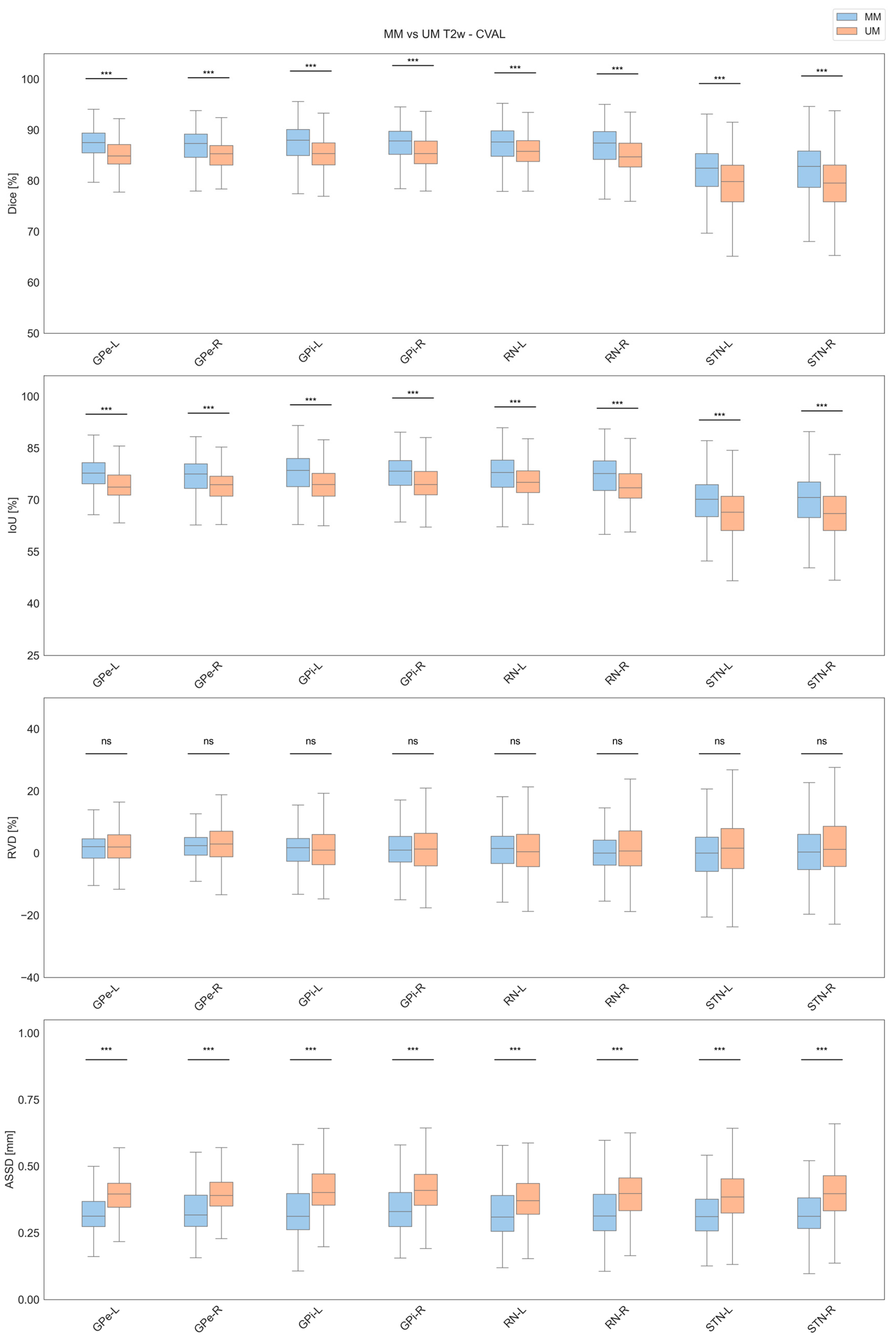
The boxplots of the T2w CVAL are shown in Figure 4, whereas the means and standard deviations are reported in Table 4. Generally, the MM consistently outperforms the T2w UM across all structures, achieving average Dice scores ranging from 80.85% to 86.63%, IoU from 68.62% to 76.95%, RVD values with a maximum overestimation of +2.41% and minimum overestimation of +0.13%, and ASSD ranging between 0.34 mm and 0.43 mm.
Regarding T1w images from CVAL, the MM model consistently achieves the highest performance for all metrics (Dice, IoU, RVD, and ASSD) on the GPe and GPi, with statistically significant improvements (p < 0.001) over the DBSegment model in all structures. The UM yields the highest performance for all metrics (Dice, IoU, RVD, and ASSD) on the RN and STN, significantly outperforming DBSegment for each evaluated metric and structure (p < 0.001).
When considering T2w images from CVAL, the MM significantly outperforms the UM (p < 0.001) in terms of Dice, IoU, and ASSD across all anatomical structures, confirming the benefit of combining T1w and T2w information. Interestingly, no statistically significant differences were found in RVD, suggesting that both models maintain comparable volumetric estimations.

3.2. Test Results

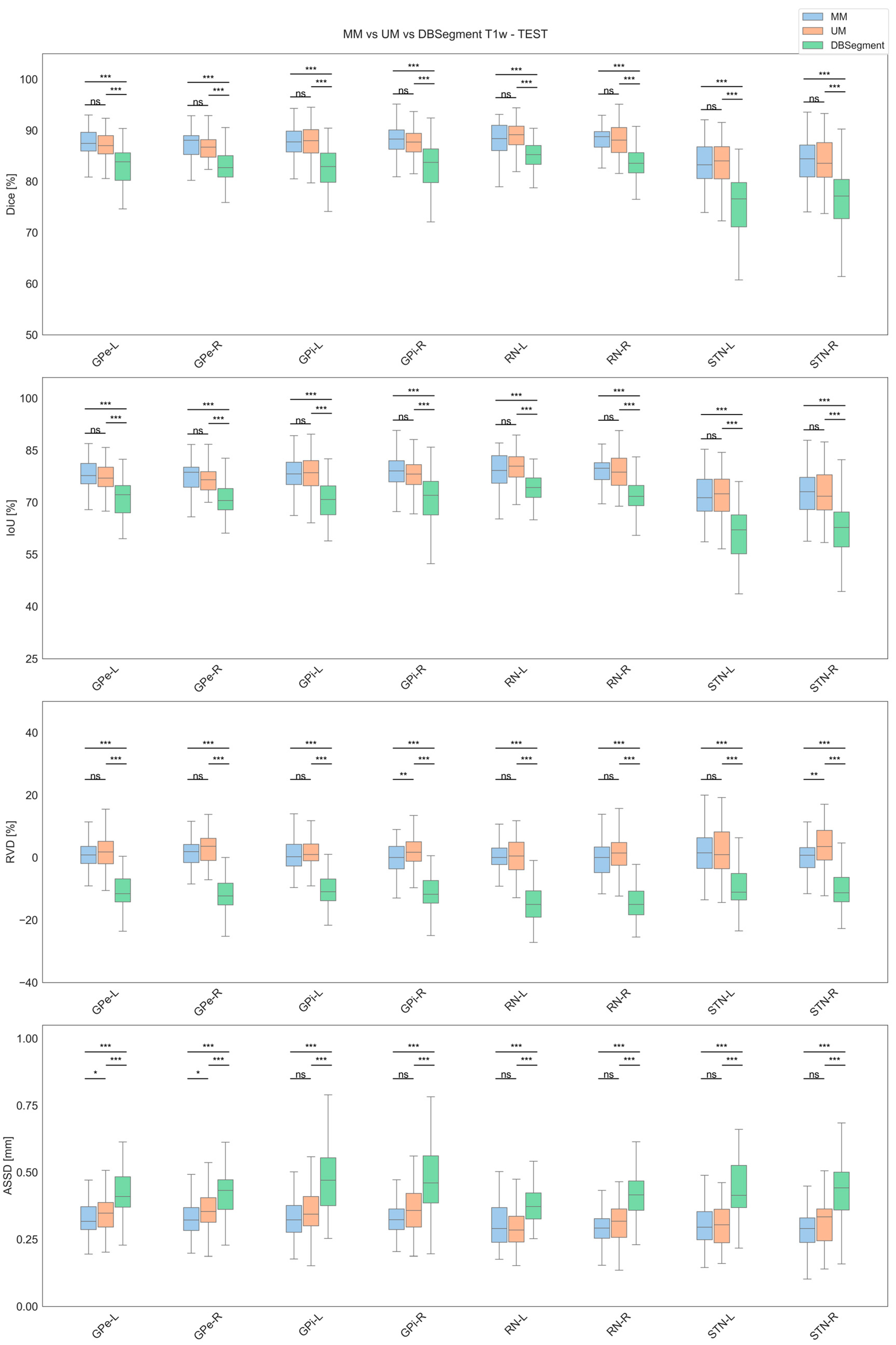
The boxplots of the T1w TEST cohort comparing all of the considered structures (GPe-L, GPe-R, GPi-L, GPi-R, RN-L, RN-R, STN-L, and STN-R), using Dice, IoU, RVD, and SSD, are pictorially depicted in Figure 5. These results are complemented by the means and standard deviations reported in Table 5. In summary, the MM and T1w UM exhibit similar performance, with all structures showing average Dice scores between 82.79% and 88.91%, IoU between 70.99% and 80.18%, RVD values not exceeding +3.45% (overestimation) or −0.46% (underestimation), and ASSD values ranging from 0.29 mm to 0.36 mm. The DBSegment model, on our TEST cohort, demonstrates a consistent trend toward volume underestimation and achieves the lowest scores across all structures.
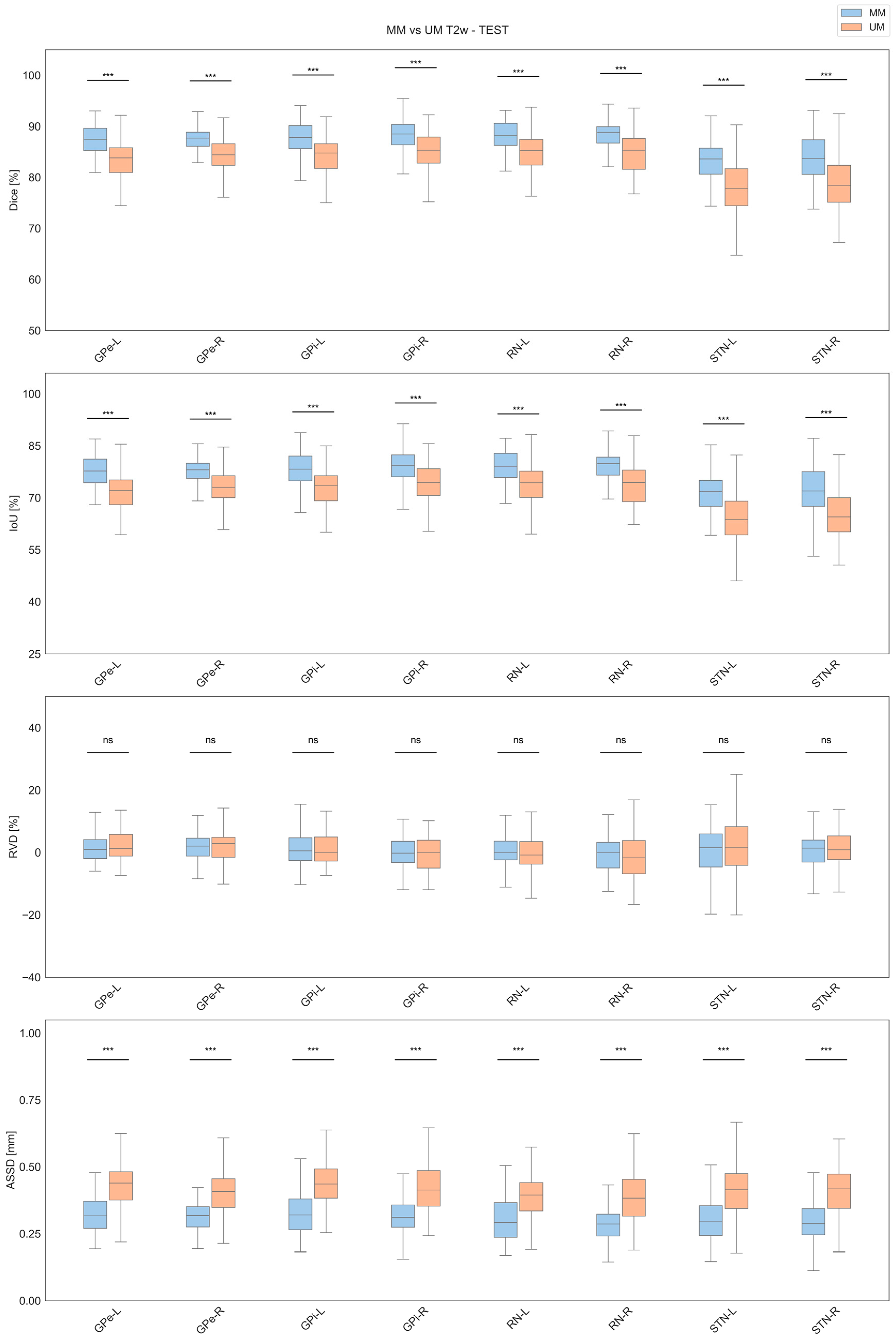
The boxplots of the T2w TEST cohort are shown in Figure 6, whereas the means and standard deviations are reported in Table 6. In general, the MM consistently outperforms the T2w UM across all structures, achieving average Dice scores ranging from 82.72% to 88.47%, IoU from 70.89% to 79.43%, RVD values with a maximum overestimation of +2.01% and maximum underestimation of −0.95%, and ASSD ranging between 0.29 mm and 0.34 mm.
Concerning T1w images from the TEST cohort, the MM model consistently achieves the highest performance across all metrics (Dice, IoU, RVD, and ASSD), with statistically significant improvements (p < 0.001) over the DBSegment model in all structures. The T1w UM yields intermediate results, significantly outperforming DBSegment for each evaluated metric and structure (p < 0.001), and achieving comparable scores to the MM ones in several cases.
Regarding T2w images, the MM significantly outperforms the T2w UM (p < 0.001) in Dice, IoU, and ASSD across all anatomical structures, confirming the benefit of combining T1w and T2w information. Interestingly, no statistically significant differences were found in RVD, suggesting that both models maintain comparable volumetric estimations.
Details of dataset-specific TEST metrics are reported in Table S1 and Table S2 for T1w and T2w images, respectively.

3.3. Qualitative Results

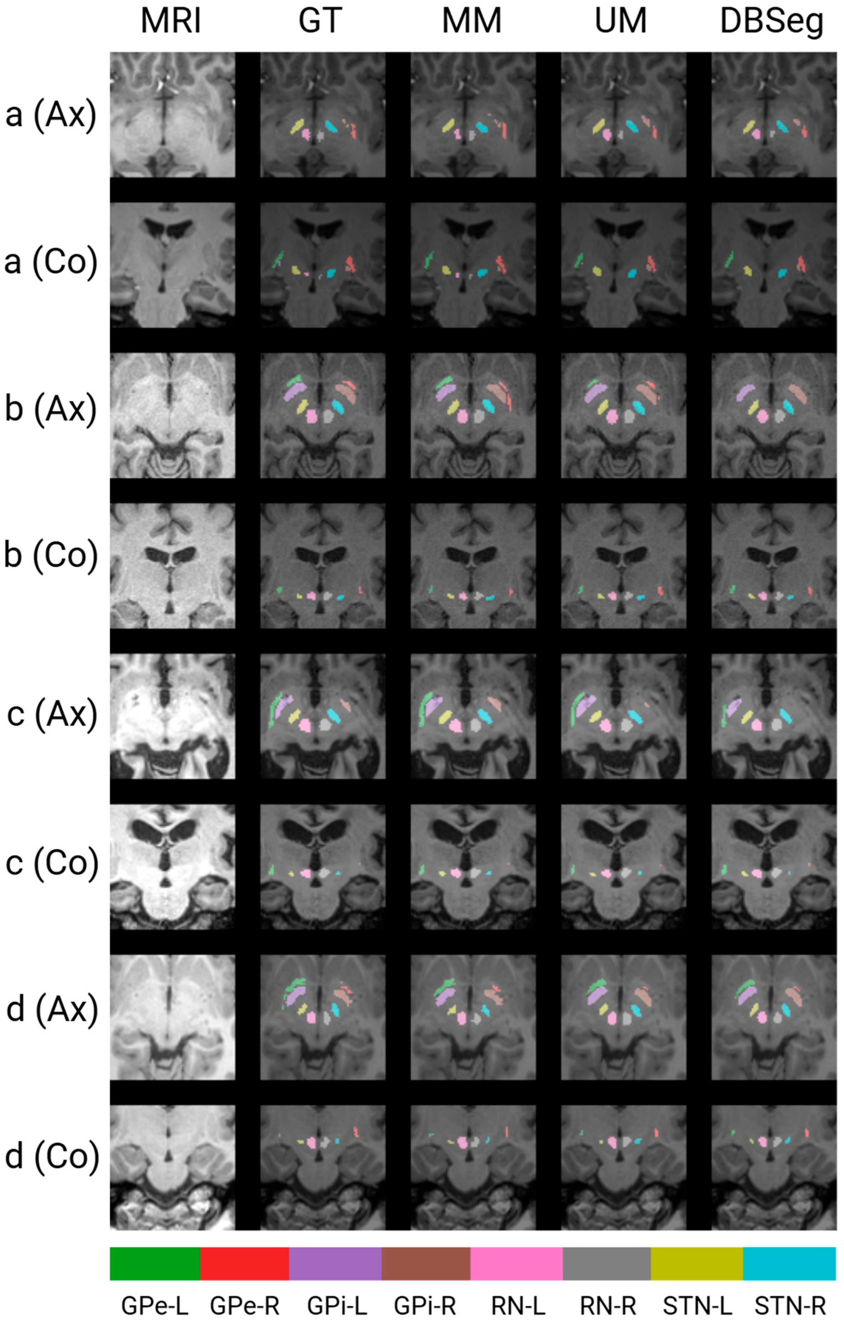
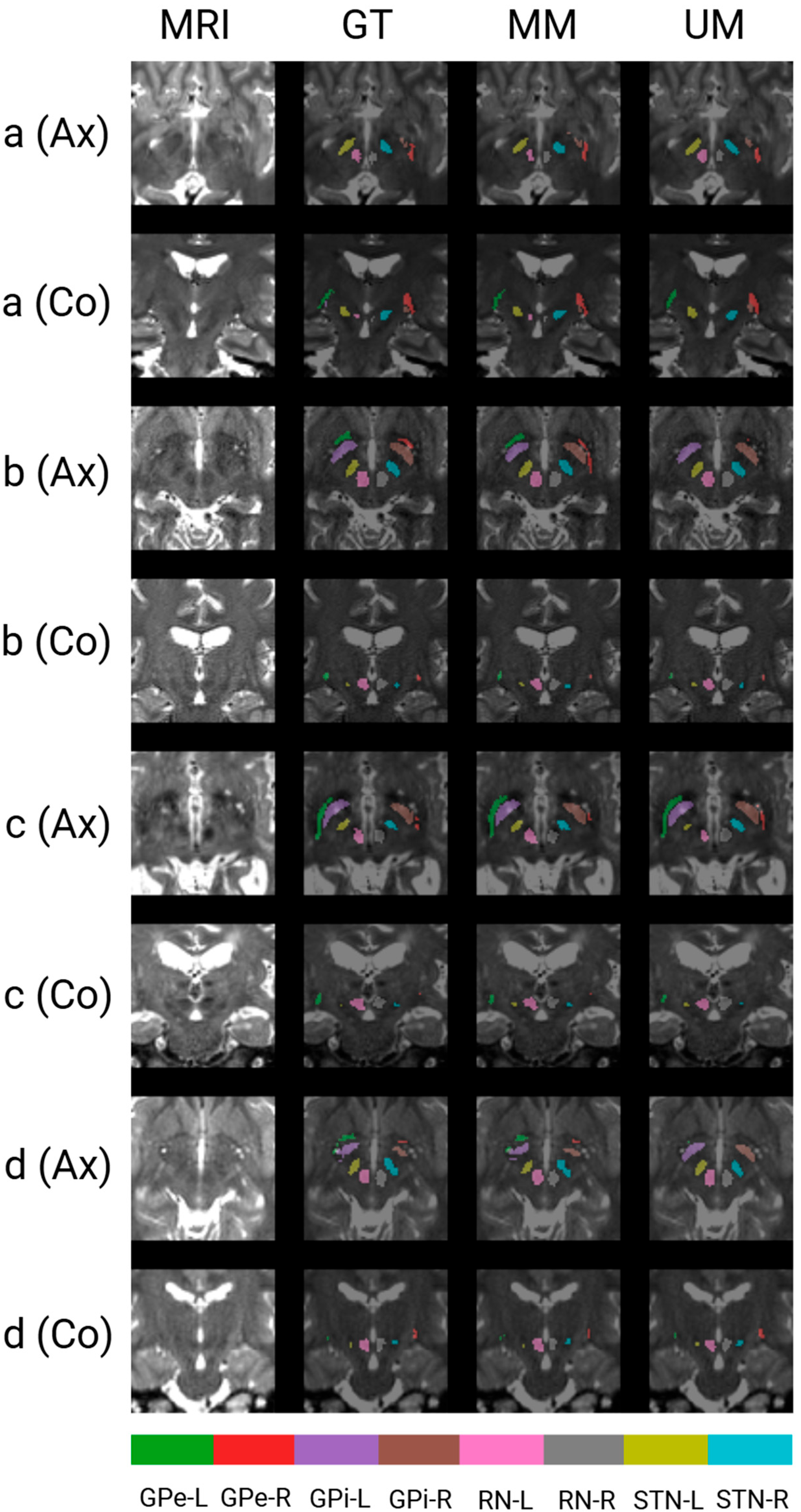
A qualitative comparison of the results of the MM, UM, and DBSegment models on the T1w TEST cohort is reported in Figure 7, which shows masks superimposed on regions of interest (ROIs) from four subjects, displayed in axial and coronal views. Every case belongs to a different collection included in the TEST cohort. Similarly, Figure 8 depicts the same ROIs extracted from T2w MRI images with the same views (axial and coronal). In this case, the comparison with DBSegment is missing, since it only supports T1w segmentation.
The segmentations predicted by all models are qualitatively accurate and visually analogous to the reference segmentations obtained using the atlas-based approach, since all structures are correctly localized. In some regions, the predicted segmentations even exhibit smoother and more anatomically plausible boundaries compared to our ground truth, possibly indicating a better generalization capability of DL models than atlas-based approaches. Moreover, the DBSegment model tends to underestimate volume predictions, as confirmed by quantitative results and the qualitative ones that are shown in Figure 7b (Ax) and Figure 7c (Ax).
Examples of the worst-case segmentations according to ASSD for T1w images are portrayed in Figure S1 and Figure S2 for the UM and MM models, respectively. Examples of the worst-case segmentations according to ASSD for T2w images are shown in Figure S3 and Figure S4 for the UM and MM models, respectively.

4. Discussion

Automated segmentation of subcortical structures is necessary for accurate diagnosis and therapy planning. Volume discrimination of adjacent structures is also a prerequisite for surgical interventions such as DBS. The most used approaches for structure segmentation are based either on local edge information, intensity, or try to combine both of them by incorporating prior shape information [44]. Structural MRI provides complementary information in the classical sequences T1w and T2w, where the first modality outlines brain structures and provides crisper images, whereas T2w highlights pathological regions, i.e., with inflammations or lesions, and renders fluids in a brighter manner.
In this study, a comprehensive comparison of UM and MM models for segmentation of deep brain structures from T1w and T2w MRI was performed. The MM approach serves as a benchmark for understanding to what extent merging these modalities affects the segmentation performance relative to the specific structural composition. Considering the Dice coefficient, as for the CVAL from T1w, the UM and MM scores are not statistically significant for 3/8 structures (GPe-L, GPe-R, and GPi-L), with the former significantly outperforming the latter for the remaining 5/8 structures (GPi-R, RN-L, RN-R, STN-L, and STN-R). These are deep, small nuclei located in the midbrain and surrounded by white matter with overlapping intensity distributions. Remarkably, an effective segmentation of the STNs through classical T1w images is also crucial in cases of neurodegenerative disorders with iron accumulation [45], where iron-sensitive sequences like susceptibility-weighted imaging and T2*w are the most employed alternative sequences. As concerns the TEST cohort from T1w, the UM and MM scores do not significantly differ for any structures but the GPe-R, in which case MM significantly outperforms UM. On the other hand, MM significantly outperformed UM from T2w on CVAL and TEST for all structures.
With regards to T1w segmentation, the proposed models (both UM and MM) significantly outperformed a reference method, DBSegment, for both the CVAL and TEST cohorts. However, no fair comparison can be carried out between DBSegment and the proposed models on T2w images, since those authors did not train on this modality.
The considerable improvement of MM over UM in T2w experiments suggests that the inclusion of T1w information effectively compensates for the lower anatomical contrast in subcortical regions, as is typically associated with T2w images. Furthermore, both MM and UM revealed comparably high performance on T1w-based segmentation, thus indicating that T1w MR images are the most relevant for segmentation of deep brain structures from a deep learning perspective.
From a clinical viewpoint, these findings are especially relevant for such neurosurgical procedures as DBS, where accurate localization of structures like the STN and GPi is critical for accurate preoperative planning, ultimately leading to improved patient outcomes.

Limitations

Despite the promising outcomes of the proposed approach, two main limitations must be acknowledged.
First, most of the MRIs included in our dataset came from either healthy subjects or patients with a condition different from Parkinson’s disease. Therefore, despite the robustness of the developed framework, as shown from our cross-validation and test experiments, it still lacks a more specific performance evaluation on the patients who are more likely to need surgical interventions for DBS. Nevertheless, the segmentation of deep brain structures remains clinically relevant not only for PD but also for other neurological conditions. In our study, patients affected by cognitive decline disorders, such as Alzheimer’s disease (AD)—for which DBS has shown potential in alleviating memory loss, a common symptom of AD [46]—have been considered. Additionally, the inclusion of patients with a history of COVID-19 offers a valuable starting point for exploring the long-term cognitive consequences of the disease. Recent evidence indicates that even individuals without a prior diagnosis of AD may experience neurodegenerative effects due to prolonged COVID-19-related hypoxia [47].
Then, our dataset was created by using registration and templates to annotate a large amount of MRI data, consisting of 325 T1w and 325 T2w images. While employing DISTAL, specifically built for DBS interventions, allowed us to obtain quality labels for this study, a validation involving neuroimaging specialists was not performed. Neuroradiologists and neurosurgeons could help in refining the dataset, providing more reliable estimates of the developed segmentation models’ performance.

5. Conclusions

This study presents a completely automated deep learning pipeline, encompassing UM and MM models, for the segmentation of eight deep brain structures that are relevant to neurosurgical procedures, especially DBS, using MRI data.
The obtained results show that the proposed UM and MM models perform better than the state-of-the-art DBSegment method on T1w MR images, on both cross-validation and an independent test set. Remarkably, no publicly available methods prior to this work exist for automatic segmentation on T2w MR images.
Future research could focus on extending the proposed pipeline to incorporate other state-of-the-art 3D segmentation models and evaluate their performance and capabilities in real-world neurosurgical environments. Collaboration with neurosurgeons would allow for more objective benchmarks for the developed models, instead of relying on ground truth generated from atlas-based approaches.
Domain adaptation, encompassing image-to-image translation [48] methods to convert T1w images to T2w images and vice versa, or even to other modalities, could be an interesting direction for future studies—for instance, exploiting generative adversarial networks [8] or diffusion models [49].
Finally, future work could also explore the use of a larger and more diverse training dataset. Particularly, datasets should be selected to include patients with PD, so that models can be more specifically tailored to DBS applications. Moreover, incorporating not only additional 3T scans but also ultra-high-field 7T MRI acquisitions, the increased spatial resolution and contrast provided by 7T imaging could enhance segmentation accuracy, particularly for small subcortical structures.

Supplementary Materials

The following are available online at https://www.mdpi.com/article/10.3390/make7030084/s1. Figure S1: Worst-case segmentations based on ASSD for the UM T1w. Figure S2: Worst-case segmentations based on ASSD for the MM T1w. Figure S3: Worst-case segmentations based on ASSD for the UM T2w. Figure S4: Worst-case segmentations based on ASSD for the MM T2w. Table S1: Dataset-specific T1w TEST metrics. Table S2: Dataset-specific T2w TEST metrics.

Author Contributions

Conceptualization, N.A.; methodology, N.A., E.L., F.G., and V.B.; software, N.A., E.L., and F.G.; validation, V.T., D.R., and G.B.; formal analysis, N.A.; investigation, N.A., E.L., F.G., M.P., V.S., and V.B.; data curation, N.A., E.L., and F.G.; writing—original draft preparation, N.A., E.L., and F.G.; writing—review and editing, N.A., E.L., F.G., M.P., V.S., L.C., and V.B.; visualization, N.A., E.L., and F.G.; supervision, V.B. All authors have read and agreed to the published version of the manuscript.

Funding

This research was funded by the NRRP project “BRIEF—Biorobotics Research and Innovation Engineering Facilities”, Mission 4: “Istruzione e Ricerca”, Component 2: “Dalla ricerca all’impresa”, Investment 3.1: “Fondo per la realizzazione di un sistema integrato di infrastrutture di ricerca e innovazione”, CUP: J13C22000400007, funded by European Union—NextGenerationEU.

Institutional Review Board Statement

Not applicable.

Data Availability Statement

MRI datasets employed for the study are available using the following links: HCP (http://www.humanconnectomeproject.org/, last accessed 9 May 2025); OASIS3 (https://sites.wustl.edu/oasisbrains/home/oasis-3/, last accessed 9 May 2025); ADNI (https://adni.loni.usc.edu/, last accessed 9 May 2025); IXI (https://brain-development.org/ixi-dataset/, last accessed 9 May 2025); UNC (https://doi.org/10.6084/m9.figshare.c.6485272.v1, last accessed 9 May 2025); THP (https://openneuro.org/datasets/ds000206/versions/1.0.0, last accessed 9 May 2025); NLA (https://openneuro.org/datasets/ds005088/versions/1.0.0, last accessed 9 May 2025); neuroCOVID (https://openneuro.org/datasets/ds005364/versions/1.0.0, last accessed 9 May 2025).

Acknowledgments

The work of Michela Prunella is supported by the Italian National Program PhD Programme in Autonomous Systems (DAuSy). The authors acknowledge the authors and curators of the HCP, OASIS3, ADNI, IXI, UNC, THP, NLA, and neuroCOVID datasets for making available the data used for this study.

Conflicts of Interest

The authors declare no conflicts of interest.

Abbreviations

The following abbreviations are used in this manuscript:
ADAlzheimer’s Disease
ADNIAlzheimer’s Disease Neuroimaging Initiative
ANTsAdvanced Normalization Tools
ASSDAverage Symmetric Surface Distance
BMBrain Mask
CVALCross-Validation Set
DLDeep Learning
DBSDeep Brain Stimulation
DISTALDBS Intrinsic Template Atlas
FLAIRFluid Attenuated Inversion Recovery
GPeGlobus Pallidus Externus
GPiGlobus Pallidus Internus
HCPHuman Connectome Project
IoUIntersection over Union
IXIInformation eXchange from Images
LPILeft–Posterior–Inferior
MMMultimodal
MNIMontreal Neurological Institute
MSDMedical Segmentation Decathlon
MRIMagnetic Resonance Imaging
NLANeural Correlates of Lidocaine Analgesic
OASIS3Open Access Series of Imaging Studies 3
PDParkinson’s Disease
RNRed Nucleus
ROIRegion of Interest
RVDRelative Volume Difference
SyNSymmetric Normalization
STNSubthalamic Nucleus
THPTraveling Human Phantom
UMUnimodal
UNCUniversity of North Carolina
T1wT1-Weighted
T2wT2-Weighted

References

  1. Liu, Y.; D’Haese, P.-F.; Newton, A.T.; Dawant, B.M. Generation of Human Thalamus Atlases from 7 T Data and Application to Intrathalamic Nuclei Segmentation in Clinical 3 T T1-Weighted Images. Magn. Reson. Imaging 2020, 65, 114–128. [Google Scholar] [CrossRef]
  2. Isaacs, B.R.; Keuken, M.C.; Alkemade, A.; Temel, Y.; Bazin, P.-L.; Forstmann, B.U. Methodological Considerations for Neuroimaging in Deep Brain Stimulation of the Subthalamic Nucleus in Parkinson’s Disease Patients. J. Clin. Med. 2020, 9, 3124. [Google Scholar] [CrossRef]
  3. Baniasadi, M.; Petersen, M.V.; Gonçalves, J.; Horn, A.; Vlasov, V.; Hertel, F.; Husch, A. DBSegment: Fast and Robust Segmentation of Deep Brain Structures Considering Domain Generalization. Hum. Brain Mapp. 2023, 44, 762–778. [Google Scholar] [CrossRef]
  4. Polanski, W.H.; Zolal, A.; Sitoci-Ficici, K.H.; Hiepe, P.; Schackert, G.; Sobottka, S.B. Comparison of Automatic Segmentation Algorithms for the Subthalamic Nucleus. Stereotact. Funct. Neurosurg. 2020, 98, 256–262. [Google Scholar] [CrossRef]
  5. Reinacher, P.C.; Várkuti, B.; Krüger, M.T.; Piroth, T.; Egger, K.; Roelz, R.; Coenen, V.A. Automatic Segmentation of the Subthalamic Nucleus: A Viable Option to Support Planning and Visualization of Patient-Specific Targeting in Deep Brain Stimulation. Oper. Neurosurg. 2019, 17, 497. [Google Scholar] [CrossRef]
  6. Chen, J.; Xu, H.; Xu, B.; Wang, Y.; Shi, Y.; Xiao, L. Automatic Localization of Key Structures for Subthalamic Nucleus–Deep Brain Stimulation Surgery via Prior-Enhanced Multi-Object Magnetic Resonance Imaging Segmentation. World Neurosurg. 2023, 178, e472–e479. [Google Scholar] [CrossRef]
  7. Kim, J.; Duchin, Y.; Sapiro, G.; Vitek, J.; Harel, N. Clinical Deep Brain Stimulation Region Prediction Using Regression Forests from High-Field MRI. In Proceedings of the 2015 IEEE International Conference on Image Processing (ICIP), Quebec City, QC, Canada, 27–30 September 2015; pp. 2480–2484. [Google Scholar]
  8. Kawahara, D.; Nagata, Y. T1-Weighted and T2-Weighted MRI Image Synthesis with Convolutional Generative Adversarial Networks. Rep. Pract. Oncol. Radiother. 2021, 26, 35–42. [Google Scholar] [CrossRef]
  9. Haegelen, C.; Coupé, P.; Fonov, V.; Guizard, N.; Jannin, P.; Morandi, X.; Collins, D.L. Automated Segmentation of Basal Ganglia and Deep Brain Structures in MRI of Parkinson’s Disease. Int. J. CARS 2013, 8, 99–110. [Google Scholar] [CrossRef]
  10. Lima, T.; Varga, I.; Bakštein, E.; Novák, D.; Alves, V. Subthalamic Nucleus Segmentation in High-Field Magnetic Resonance Data. Is Space Normalization by Template Co-Registration Necessary? arXiv 2024, arXiv:2407.15485. [Google Scholar]
  11. Pauli, W.M.; Nili, A.N.; Tyszka, J.M. A High-Resolution Probabilistic in Vivo Atlas of Human Subcortical Brain Nuclei. Sci. Data 2018, 5, 180063. [Google Scholar] [CrossRef]
  12. Ewert, S.; Plettig, P.; Li, N.; Chakravarty, M.M.; Collins, D.L.; Herrington, T.M.; Kühn, A.A.; Horn, A. Toward Defining Deep Brain Stimulation Targets in MNI Space: A Subcortical Atlas Based on Multimodal MRI, Histology and Structural Connectivity. NeuroImage 2018, 170, 271–282. [Google Scholar] [CrossRef]
  13. Su, J.H.; Thomas, F.T.; Kasoff, W.S.; Tourdias, T.; Choi, E.Y.; Rutt, B.K.; Saranathan, M. Thalamus Optimized Multi Atlas Segmentation (THOMAS): Fast, Fully Automated Segmentation of Thalamic Nuclei from Structural MRI. NeuroImage 2019, 194, 272–282. [Google Scholar] [CrossRef]
  14. Brett, M.; Johnsrude, I.S.; Owen, A.M. The Problem of Functional Localization in the Human Brain. Nat. Rev. Neurosci. 2002, 3, 243–249. [Google Scholar] [CrossRef]
  15. Horn, A.; Kühn, A.A. Lead-DBS: A Toolbox for Deep Brain Stimulation Electrode Localizations and Visualizations. NeuroImage 2015, 107, 127–135. [Google Scholar] [CrossRef]
  16. Horn, A.; Li, N.; Dembek, T.A.; Kappel, A.; Boulay, C.; Ewert, S.; Tietze, A.; Husch, A.; Perera, T.; Neumann, W.-J.; et al. Lead-DBS v2: Towards a Comprehensive Pipeline for Deep Brain Stimulation Imaging. NeuroImage 2019, 184, 293–316. [Google Scholar] [CrossRef]
  17. Neudorfer, C.; Butenko, K.; Oxenford, S.; Rajamani, N.; Achtzehn, J.; Goede, L.; Hollunder, B.; Ríos, A.S.; Hart, L.; Tasserie, J.; et al. Lead-DBS v3.0: Mapping Deep Brain Stimulation Effects to Local Anatomy and Global Networks. NeuroImage 2023, 268, 119862. [Google Scholar] [CrossRef]
  18. Xiao, Y.; Fonov, V.S.; Beriault, S.; Gerard, I.; Sadikot, A.F.; Pike, G.B.; Collins, D.L. Patch-Based Label Fusion Segmentation of Brainstem Structures with Dual-Contrast MRI for Parkinson’s Disease. Int. J. CARS 2015, 10, 1029–1041. [Google Scholar] [CrossRef]
  19. Falahati, F.; Gustavsson, J.; Kalpouzos, G. Automated Segmentation of Midbrain Nuclei Using Deep Learning and Multisequence MRI: A Longitudinal Study on Iron Accumulation with Age. Imaging Neurosci. 2024, 2, 1–20. [Google Scholar] [CrossRef]
  20. Altini, N.; Rossini, M.; Turkevi-Nagy, S.; Pesce, F.; Pontrelli, P.; Prencipe, B.; Berloco, F.; Seshan, S.; Gibier, J.-B.; Pedraza Dorado, A.; et al. Performance and Limitations of a Supervised Deep Learning Approach for the Histopathological Oxford Classification of Glomeruli with IgA Nephropathy. Comput. Methods Programs Biomed. 2023, 242, 107814. [Google Scholar] [CrossRef]
  21. Bevilacqua, V.; Altini, N.; Prencipe, B.; Brunetti, A.; Villani, L.; Sacco, A.; Morelli, C.; Ciaccia, M.; Scardapane, A. Lung Segmentation and Characterization in COVID-19 Patients for Assessing Pulmonary Thromboembolism: An Approach Based on Deep Learning and Radiomics. Electronics 2021, 10, 2475. [Google Scholar] [CrossRef]
  22. Berloco, F.; Zaccaria, G.M.; Altini, N.; Colucci, S.; Bevilacqua, V. A Multimodal Framework for Assessing the Link between Pathomics, Transcriptomics, and Pancreatic Cancer Mutations. Comput. Med. Imaging Graph. 2025, 123, 102526. [Google Scholar] [CrossRef]
  23. Isensee, F.; Jaeger, P.F.; Kohl, S.A.A.; Petersen, J.; Maier-Hein, K.H. nnU-Net: A Self-Configuring Method for Deep Learning-Based Biomedical Image Segmentation. Nat. Methods 2021, 18, 203–211. [Google Scholar] [CrossRef]
  24. Altini, N.; Brunetti, A.; Napoletano, V.P.; Girardi, F.; Allegretti, E.; Hussain, S.M.; Brunetti, G.; Triggiani, V.; Bevilacqua, V.; Buongiorno, D. A Fusion Biopsy Framework for Prostate Cancer Based on Deformable Superellipses and nnU-Net. Bioengineering 2022, 9, 343. [Google Scholar] [CrossRef]
  25. Solomon, O.; Palnitkar, T.; Patriat, R.; Braun, H.; Aman, J.; Park, M.C.; Vitek, J.; Sapiro, G.; Harel, N. Deep-learning Based Fully Automatic Segmentation of the Globus Pallidus Interna and Externa Using Ultra-high 7 Tesla MRI. Hum. Brain Mapp. 2021, 42, 2862–2879. [Google Scholar] [CrossRef]
  26. Beliveau, V.; Nørgaard, M.; Birkl, C.; Seppi, K.; Scherfler, C. Automated Segmentation of Deep Brain Nuclei Using Convolutional Neural Networks and Susceptibility Weighted Imaging. Hum. Brain Mapp. 2021, 42, 4809–4822. [Google Scholar] [CrossRef]
  27. Hanke, M.; Baumgartner, F.J.; Ibe, P.; Kaule, F.R.; Pollmann, S.; Speck, O.; Zinke, W.; Stadler, J. A High-Resolution 7-Tesla fMRI Dataset from Complex Natural Stimulation with an Audio Movie. Sci. Data 2014, 1, 140003. [Google Scholar] [CrossRef]
  28. Van Essen, D.C.; Ugurbil, K.; Auerbach, E.; Barch, D.; Behrens, T.E.J.; Bucholz, R.; Chang, A.; Chen, L.; Corbetta, M.; Curtiss, S.W.; et al. The Human Connectome Project: A Data Acquisition Perspective. NeuroImage 2012, 62, 2222–2231. [Google Scholar] [CrossRef]
  29. LaMontagne, P.J.; Benzinger, T.L.S.; Morris, J.C.; Keefe, S.; Hornbeck, R.; Xiong, C.; Grant, E.; Hassenstab, J.; Moulder, K.; Vlassenko, A.G.; et al. OASIS-3: Longitudinal Neuroimaging, Clinical, and Cognitive Dataset for Normal Aging and Alzheimer Disease. medRxiv 2019. [Google Scholar] [CrossRef]
  30. Mueller, S.G.; Weiner, M.W.; Thal, L.J.; Petersen, R.C.; Jack, C.R.; Jagust, W.; Trojanowski, J.Q.; Toga, A.W.; Beckett, L. Ways toward an Early Diagnosis in Alzheimer’s Disease: The Alzheimer’s Disease Neuroimaging Initiative (ADNI). Alzheimers Dement. 2005, 1, 55–66. [Google Scholar] [CrossRef]
  31. IXI Dataset—Brain Development. Available online: https://brain-development.org/ixi-dataset/ (accessed on 15 June 2025).
  32. Chen, X.; Qu, L.; Xie, Y.; Ahmad, S.; Yap, P.-T. A Paired Dataset of T1- and T2-Weighted MRI at 3 Tesla and 7 Tesla. Sci. Data 2023, 10, 489. [Google Scholar] [CrossRef]
  33. Magnotta, V.A.; Matsui, J.T.; Liu, D.; Johnson, H.J.; Long, J.D.; Bolster, B.D.; Mueller, B.A.; Lim, K.; Mori, S.; Helmer, K.G.; et al. MultiCenter Reliability of Diffusion Tensor Imaging. Brain Connect. 2012, 2, 345–355. [Google Scholar] [CrossRef]
  34. Vogt, K.M.; Burlew, A.C.; Simmons, M.A.; Reddy, S.N.; Kozdron, C.N.; Ibinson, J.W. Neural Correlates of Systemic Lidocaine Administration in Healthy Adults Measured by Functional MRI: A Single Arm Open Label Study. Br. J. Anaesth. 2025, 134, 414–424. [Google Scholar] [CrossRef]
  35. Kausel, L.; Figueroa-Vargas, A.; Zamorano, F.; Stecher, X.; Aspé-Sánchez, M.; Carvajal-Paredes, P.; Márquez-Rodríguez, V.; Martínez-Molina, M.P.; Román, C.; Soto-Fernández, P.; et al. Patients Recovering from COVID-19 Who Presented with Anosmia during Their Acute Episode Have Behavioral, Functional, and Structural Brain Alterations. Sci. Rep. 2024, 14, 19049. [Google Scholar] [CrossRef]
  36. Fonov, V.S.; Evans, A.C.; McKinstry, R.C.; Almli, C.R.; Collins, D.L. Unbiased Nonlinear Average Age-Appropriate Brain Templates from Birth to Adulthood. NeuroImage 2009, 47, S102. [Google Scholar] [CrossRef]
  37. 3D Slicer Image Computing Platform. Available online: https://slicer.org/ (accessed on 21 May 2025).
  38. Baek, H.-M. Diffusion Measures of Subcortical Structures Using High-Field MRI. Brain Sci. 2023, 13, 391. [Google Scholar] [CrossRef]
  39. Tustison, N.J.; Avants, B.B.; Cook, P.A.; Zheng, Y.; Egan, A.; Yushkevich, P.A.; Gee, J.C. N4ITK: Improved N3 Bias Correction. IEEE Trans. Med. Imaging 2010, 29, 1310–1320. [Google Scholar] [CrossRef]
  40. Avants, B.; Epstein, C.; Grossman, M.; Gee, J. Symmetric Diffeomorphic Image Registration with Cross-Correlation: Evaluating Automated Labeling of Elderly and Neurodegenerative Brain. Med. Image Anal. 2008, 12, 26–41. [Google Scholar] [CrossRef]
  41. Gulban, O.F.; Nielson, D.; Lee, J.; Poldrack, R.; Gorgolewski, C.; Vanessasaurus; Markiewicz, C. Poldracklab/Pydeface: PyDeface, version 2.0.2; Zenodo: Geneva, Switzerland, 2022.
  42. Altini, N.; Prencipe, B.; Cascarano, G.D.; Brunetti, A.; Brunetti, G.; Triggiani, V.; Carnimeo, L.; Marino, F.; Guerriero, A.; Villani, L.; et al. Liver, Kidney and Spleen Segmentation from CT Scans and MRI with Deep Learning: A Survey. Neurocomputing 2022, 490, 30–53. [Google Scholar] [CrossRef]
  43. Benjamini, Y.; Hochberg, Y. Controlling the False Discovery Rate: A Practical and Powerful Approach to Multiple Testing. J. R. Stat. Soc. Ser. B Stat. Methodol. 1995, 57, 289–300. [Google Scholar] [CrossRef]
  44. Kim, J.; Lenglet, C.; Duchin, Y.; Sapiro, G.; Harel, N. Semiautomatic Segmentation of Brain Subcortical Structures From High-Field MRI. IEEE J. Biomed. Health Inform. 2014, 18, 1678–1695. [Google Scholar] [CrossRef]
  45. Lee, J.-H.; Yun, J.Y.; Gregory, A.; Hogarth, P.; Hayflick, S.J. Brain MRI Pattern Recognition in Neurodegeneration With Brain Iron Accumulation. Front. Neurol. 2020, 11, 1024. [Google Scholar] [CrossRef] [PubMed]
  46. Hescham, S.; Lim, L.W.; Jahanshahi, A.; Blokland, A.; Temel, Y. Deep Brain Stimulation in Dementia-Related Disorders. Neurosci. Biobehav. Rev. 2013, 37, 2666–2675. [Google Scholar] [CrossRef] [PubMed]
  47. Links Between COVID-19 and Parkinson’s Disease/Alzheimer’s Disease: Reciprocal Impacts, Medical Care Strategies and Underlying Mechanisms | Translational Neurodegeneration | Full Text. Available online: https://translationalneurodegeneration.biomedcentral.com/articles/10.1186/s40035-023-00337-1 (accessed on 9 July 2025).
  48. Altini, N.; Marvulli, T.M.; Zito, F.A.; Caputo, M.; Tommasi, S.; Azzariti, A.; Brunetti, A.; Prencipe, B.; Mattioli, E.; De Summa, S.; et al. The Role of Unpaired Image-to-Image Translation for Stain Color Normalization in Colorectal Cancer Histology Classification. Comput. Methods Programs Biomed. 2023, 234, 107511. [Google Scholar] [CrossRef] [PubMed]
  49. Dayarathna, S.; Islam, K.T.; Zhuang, B.; Yang, G.; Cai, J.; Law, M.; Chen, Z. McCaD: Multi-Contrast MRI Conditioned, Adaptive Adversarial Diffusion Model for High-Fidelity MRI Synthesis. In Proceedings of the 2025 IEEE/CVF Winter Conference on Applications of Computer Vision (WACV), Tucson, AZ, USA, 28 February–4 March 2025; pp. 670–679. [Google Scholar]
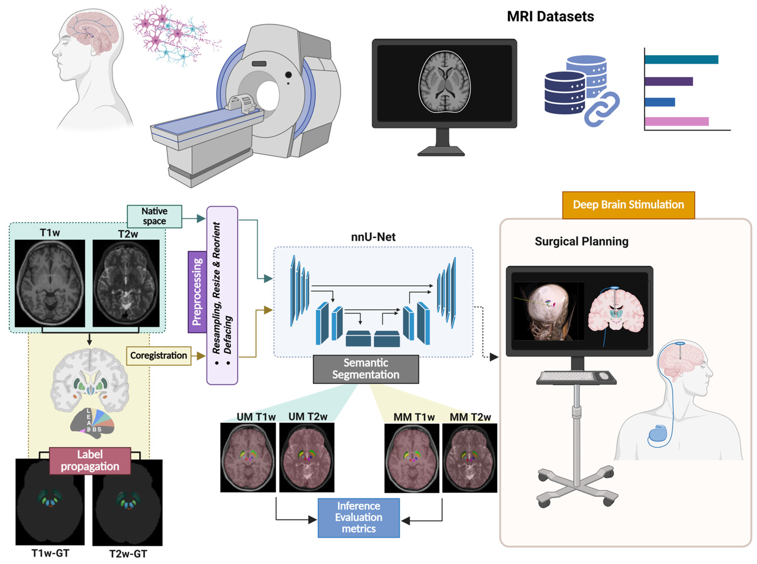
Figure 1. Overview of the study workflow: After data acquisition and data annotation, a preprocessing pipeline standardizes the images via defacing, resampling, and reorientation. The resulting datasets are used to train and evaluate three nnU-Net models (two unimodal models, UM T1w and UM T2w; and a multimodal model, MM) for automated segmentation of deep brain structures for neurosurgical planning.
Make 07 00084 g001
Figure 2. Network architecture: The architecture was optimized through the nnU-Net framework. The diagram shows a six-stage 3D full-resolution U-Net with an encoder–decoder structure. The legend highlights key components: purple numbers indicate the number of feature maps (represented by the blue blocks); orange text shows the size of the convolutional kernels (3 × 3 × 3) and their stride, followed by instance normalization and Leaky ReLU; red and green arrows denote downsampling and upsampling operations, respectively; dashed arrows indicate skip connections. For each level, the spatial dimensions and voxel spacing of the corresponding feature maps are also reported. The input patch size is 128 × 160 × 112, extracted from images with a median size of MX × MY × MZ after nnU-Net’s automatic cropping during preprocessing. The same architecture was employed for all three models (MM, UM T1w, and UM T2w), with differences only in the number of input channels and median image dimensions (200 × 237 × 186 for MM, 250 × 254 × 191.5 for UM T1w, and 241 × 241.5 × 191.5 for UM T2w). The final 1 × 1 × 1 convolution, followed by a softmax activation, produces the output segmentation map.
Make 07 00084 g002
Figure 3. Boxplots for T1w images from the CVAL cohort. Dice, IoU, RVD, and ASSD metrics, for each segmented anatomical structure (columns), as obtained from the models under comparison. Horizontal bars indicate the statistical significance between model pairs, assessed using the Wilcoxon signed-rank test: ** for p-values < 0.01, and *** for p-values < 0.001; ‘ns’ denotes non-significant differences.
Make 07 00084 g003
Figure 4. Boxplots for T2w images from the CVAL cohort. Dice, IoU, RVD, and ASSD metrics, for each segmented anatomical structure (columns), as obtained from the models under comparison. Horizontal bars indicate the statistical significance between model pairs, assessed using the Wilcoxon signed-rank test: *** for p-values < 0.001; ‘ns’ denotes non-significant differences.
Make 07 00084 g004
Figure 5. Boxplots for T1w images from the TEST cohort. Dice, IoU, RVD, and ASSD metrics, for each segmented anatomical structure (columns), as obtained from the models under comparison. Horizontal bars indicate the statistical significance between model pairs, assessed using the Wilcoxon signed-rank test: * for p-values < 0.05, ** for p-values < 0.01, and *** for p-values < 0.001; ‘ns’ denotes non-significant differences.
Make 07 00084 g005
Figure 6. Boxplots for T2w images from the TEST cohort. Dice, IoU, RVD, and ASSD metrics, for each segmented anatomical structure (columns), as obtained from the models under comparison. Horizontal bars indicate the statistical significance between model pairs, assessed using the Wilcoxon signed-rank test: *** for p-values < 0.001; ‘ns’ denotes non-significant differences.
Make 07 00084 g006
Figure 7. Qualitative comparison on the T1w images from the TEST cohort. Columns: MRI raw image, ground truth, MM, UM, and DBSegment predictions. Rows: axial and coronal views of 4 subjects from (a) neuroCOVID (b) ADNI4 (c) OASIS3 (d) IXI datasets.
Make 07 00084 g007
Figure 8. Qualitative comparison on the T2w images from the TEST cohort. Columns: MRI raw image, ground truth, MM, and UM predictions. Rows: axial and coronal views of 4 subjects from (a) neuroCOVID (b) ADNI4 (c) OASIS3 (d) IXI datasets.
Make 07 00084 g008
Table 1. Details of the study datasets. Acronyms: CVAL (cross-validation set), TEST (test set), HCP (Human Connectome Project), OASIS3 (Open Access Series of Imaging Studies 3), ADNI (Alzheimer’s Disease Neuroimaging Initiative), IXI (Information eXchange from Images), UNC (University of North Carolina), THP (Traveling Human Phantom), NLA (Neural Correlates of Lidocaine Analgesic), SM (Siemens), PL (Philips), FS (Field Strength), T1w (T1-weighted), MPRAGE (Magnetization Prepared RApid Gradient Echo), T2w (T2-weighted), SPACE (Sampling Perfection with Application Optimized Contrast Using Different Flip Angle Evolution), VISTA (Volume ISotropic Turbo Spin Echo Acquisition), TSE (Turbo Spin Echo), HT (healthy), MCI (Mild Cognitive Impairment), CI (Cognitive Impairment), AD (Alzheimer’s disease), RI (Respiratory Infection), M/F (male/female), N/A (not available).
SubsetDatasetScannerFST1wT2wDiseaseAgeM/FMRI Scans
CVAL
(n = 260)
HCPSM3TMPRAGESPACEHTN/A16/1329
OASIS3SM3TMPRAGESPACEHT, CI52–8411/1930
ADNI4PL, SM3TMPRAGESPACE/VISTAHT, MCI, AD55–8513/4659
IXIN/AN/AN/AN/AHT21–7416/1329
UNCSM3T, 7TMPRAGE, MP2RAGESPACE,
TSE
HT25–4111/516
THPPL, SM3TMPRAGESPACEHTN/AN/A40
NLASM3TMPRAGESPACEHT20–5513/1427
neuroCOVIDSM3TMPRAGESPACECOVID, RI21–6417/1330
TEST
(n = 65)
OASIS3SM3TMPRAGESPACEHT, CI59–975/1116
ADNI4SM3TMPRAGESPACEHT, MCI, AD56–857/916
IXIN/AN/AN/AN/AHT23–639/817
neuroCOVIDSM3TMPRAGESPACECOVID, RI19–669/716
Table 2. Considered deep brain structures for this study. Full name, acronym, and label values are reported for each of the structures included in our segmentation models.
Full NameAcronymLabel
Brain maskBM1
Globus pallidus externus (left)GPe-L2
Globus pallidus externus (right)GPe-R3
Globus pallidus internus (left)GPi-L4
Globus pallidus internus (right)GPi-R5
Red nucleus (left)RN-L6
Red nucleus (right)RN-R7
Subthalamic nucleus (left)STN-L8
Subthalamic nucleus (right)STN-R9
Table 3. T1w CVAL metrics: Dice, IoU, RVD, and ASSD are reported in terms of mean ± standard deviation for each considered anatomical structure.
LabelModelDice [%]IoU [%]RVD [%]ASSD [mm]
BMMM98.18 ± 0.4996.44 ± 0.920.10 ± 1.230.68 ± 0.17
UM98.14 ± 0.5896.36 ± 1.080.46 ± 1.420.72 ± 0.20
DBSegment96.31 ± 0.7092.89 ± 1.281.21 ± 2.321.52 ± 0.77
GPe-LMM86.48 ± 7.2876.71 ± 8.371.77 ± 5.930.43 ± 1.44
UM86.49 ± 6.0776.56 ± 7.101.47 ± 8.720.38 ± 0.38
DBSegment81.30 ± 4.6768.74 ± 6.37−9.84 ± 8.650.48 ± 0.17
GPe-RMM85.91 ± 6.9675.80 ± 8.572.29 ± 5.080.40 ± 0.73
UM86.72 ± 4.5576.81 ± 6.392.14 ± 6.510.35 ± 0.11
DBSegment81.66 ± 4.7669.27 ± 6.58−12.17 ± 7.930.49 ± 0.47
GPi-LMM86.74 ± 7.2877.12 ± 8.601.30 ± 7.310.43 ± 1.34
UM87.44 ± 4.6277.95 ± 6.431.08 ± 8.030.36 ± 0.16
DBSegment81.13 ± 5.6668.61 ± 7.56−10.43 ± 7.520.51 ± 0.15
GPi-RMM86.39 ± 7.0976.57 ± 8.821.60 ± 6.430.40 ± 0.64
UM87.91 ± 3.7578.61 ± 5.761.54 ± 7.280.35 ± 0.10
DBSegment81.23 ± 5.9268.79 ± 8.01−12.05 ± 7.400.52 ± 0.21
RN-LMM86.23 ± 7.2476.37 ± 9.311.20 ± 9.830.36 ± 0.19
UM87.97 ± 8.4879.18 ± 8.971.70 ± 8.110.35 ± 0.59
DBSegment83.10 ± 4.8671.38 ± 6.90−14.88 ± 7.520.43 ± 0.12
RN-RMM86.11 ± 6.2976.08 ± 8.73−0.01 ± 7.510.35 ± 0.15
UM87.92 ± 8.5679.10 ± 9.031.45 ± 7.820.35 ± 0.64
DBSegment82.34 ± 5.3170.31 ± 7.41−15.66 ± 7.310.44 ± 0.13
STN-LMM80.93 ± 8.9668.74 ± 10.480.27 ± 9.140.40 ± 0.89
UM83.15 ± 7.3371.72 ± 9.122.13 ± 9.970.36 ± 0.53
DBSegment75.14 ± 7.6160.76 ± 9.58−12.68 ± 8.940.45 ± 0.14
STN-RMM81.27 ± 8.4369.18 ± 10.320.37 ± 8.590.37 ± 0.38
UM83.29 ± 7.4271.91 ± 8.822.14 ± 9.650.39 ± 1.07
DBSegment75.75 ± 7.9961.60 ± 9.97−13.64 ± 8.510.46 ± 0.15
Table 4. T2w CVAL metrics: Dice, IoU, RVD, and ASSD are reported in terms of mean ± standard deviation for each considered anatomical structure.
LabelModelDice [%]IoU [%]RVD [%]ASSD [mm]
BMMM98.18 ± 0.4996.44 ± 0.910.09 ± 1.220.67 ± 0.17
UM98.07 ± 0.5696.22 ± 1.040.21 ± 1.470.74 ± 0.19
GPe-LMM86.39 ± 7.2776.56 ± 8.401.65 ± 6.080.42 ± 1.44
UM84.36 ± 6.6773.36 ± 7.401.22 ± 9.960.45 ± 0.61
GPe-RMM85.90 ± 6.9075.79 ± 8.552.41 ± 5.240.39 ± 0.71
UM84.92 ± 3.3673.94 ± 4.972.90 ± 6.860.40 ± 0.09
GPi-LMM86.63 ± 7.3476.95 ± 8.711.45 ± 7.480.43 ± 1.35
UM84.76 ± 6.5573.95 ± 7.341.11 ± 10.650.41 ± 0.11
GPi-RMM86.48 ± 6.9076.71 ± 8.751.56 ± 6.690.39 ± 0.63
UM85.34 ± 3.8974.62 ± 5.702.25 ± 9.560.46 ± 0.60
RN-LMM86.20 ± 7.6176.37 ± 9.601.09 ± 9.750.35 ± 0.21
UM85.54 ± 4.3474.97 ± 6.261.40 ± 9.970.38 ± 0.10
RN-RMM86.09 ± 6.1776.04 ± 8.640.13 ± 8.020.34 ± 0.15
UM84.73 ± 3.9873.70 ± 5.891.81 ± 9.590.40 ± 0.10
STN-LMM80.85 ± 8.9168.62 ± 10.480.14 ± 9.790.38 ± 0.86
UM78.92 ± 6.6365.63 ± 8.321.88 ± 12.590.40 ± 0.16
STN-RMM81.13 ± 8.6369.00 ± 10.600.67 ± 8.730.36 ± 0.37
UM79.45 ± 5.7466.29 ± 7.902.54 ± 11.180.40 ± 0.11
Table 5. T1w TEST metrics: Dice, IoU, RVD, and ASSD are reported in terms of mean ± standard deviation for each considered anatomical structure.
LabelModelDice [%]IoU [%]RVD [%]ASSD [mm]
BMMM98.24 ± 0.4196.54 ± 0.79−0.25 ± 1.200.67 ± 0.15
UM98.19 ± 0.5496.45 ± 1.020.34 ± 1.560.70 ± 0.20
DBSegment96.31 ± 0.5992.88 ± 1.08−0.00 ± 2.021.42 ± 0.21
GPe-LMM86.76 ± 4.0176.83 ± 5.871.81 ± 6.130.34 ± 0.10
UM86.93 ± 2.9677.00 ± 4.611.48 ± 6.170.35 ± 0.07
DBSegment82.44 ± 4.8670.40 ± 6.62−10.84 ± 5.690.44 ± 0.12
GPe-RMM86.88 ± 3.9577.01 ± 5.911.83 ± 5.190.34 ± 0.10
UM86.48 ± 3.5476.34 ± 5.392.42 ± 5.460.36 ± 0.09
DBSegment82.04 ± 5.4369.88 ± 7.44−11.44 ± 7.470.52 ± 0.66
GPi-LMM87.39 ± 3.8077.80 ± 5.821.70 ± 6.150.34 ± 0.10
UM87.53 ± 3.5478.00 ± 5.551.51 ± 5.120.35 ± 0.09
DBSegment82.52 ± 4.3170.46 ± 6.16−10.10 ± 5.310.47 ± 0.11
GPi-RMM88.01 ± 3.4378.75 ± 5.400.23 ± 5.360.33 ± 0.09
UM87.68 ± 3.1278.20 ± 4.941.84 ± 5.440.36 ± 0.09
DBSegment83.04 ± 4.8971.29 ± 7.05−10.98 ± 5.750.48 ± 0.20
RN-LMM88.17 ± 3.2178.98 ± 5.050.06 ± 5.550.31 ± 0.08
UM88.91 ± 3.1280.18 ± 5.020.25 ± 6.070.29 ± 0.08
DBSegment84.69 ± 3.5773.61 ± 5.16−14.61 ± 6.140.39 ± 0.09
RN-RMM88.29 ± 2.5979.12 ± 4.12−0.46 ± 5.130.30 ± 0.07
UM88.08 ± 3.4078.87 ± 5.441.13 ± 5.890.31 ± 0.08
DBSegment83.42 ± 3.2571.69 ± 4.77−14.63 ± 5.290.42 ± 0.08
STN-LMM82.79 ± 5.5570.99 ± 7.632.09 ± 8.180.31 ± 0.09
UM83.37 ± 4.5371.73 ± 6.622.21 ± 7.240.31 ± 0.08
DBSegment75.44 ± 6.2060.95 ± 7.86−10.03 ± 6.810.44 ± 0.11
STN-RMM83.86 ± 4.9572.50 ± 7.190.60 ± 6.940.30 ± 0.09
UM84.01 ± 4.5872.69 ± 6.833.45 ± 6.640.31 ± 0.09
DBSegment76.45 ± 6.7262.34 ± 8.68−10.13 ± 6.200.44 ± 0.12
Table 6. T2w TEST metrics: Dice, IoU, RVD, and ASSD are reported in terms of mean ± standard deviation for each considered anatomical structure.
LabelModelDice [%]IoU [%]RVD [%]ASSD [mm]
BMMM98.24 ± 0.4196.54 ± 0.78−0.25 ± 1.200.66 ± 0.15
UM98.10 ± 0.5196.27 ± 0.97−0.10 ± 1.480.73 ± 0.19
GPe-LMM86.74 ± 4.0976.79 ± 5.972.01 ± 6.190.34 ± 0.10
UM82.49 ± 8.1670.83 ± 9.320.70 ± 12.610.52 ± 0.64
GPe-RMM86.93 ± 3.8777.08 ± 5.781.96 ± 5.270.34 ± 0.10
UM84.38 ± 3.6973.16 ± 5.491.86 ± 5.080.41 ± 0.09
GPi-LMM87.30 ± 3.8977.66 ± 5.941.83 ± 5.970.34 ± 0.10
UM83.24 ± 7.2871.83 ± 8.96−0.21 ± 11.180.48 ± 0.27
GPi-RMM88.06 ± 3.5178.83 ± 5.510.19 ± 5.610.33 ± 0.09
UM84.74 ± 4.6173.78 ± 6.600.18 ± 7.800.52 ± 0.75
RN-LMM88.16 ± 3.2078.97 ± 5.040.37 ± 6.060.30 ± 0.08
UM84.81 ± 4.8573.92 ± 7.13−0.18 ± 7.140.40 ± 0.12
RN-RMM88.47 ± 2.7179.43 ± 4.33−0.95 ± 5.200.29 ± 0.07
UM85.06 ± 4.1974.23 ± 6.38−1.43 ± 7.620.38 ± 0.10
STN-LMM82.72 ± 5.6970.89 ± 7.761.26 ± 8.320.30 ± 0.09
UM77.75 ± 5.8263.97 ± 7.751.80 ± 10.760.41 ± 0.10
STN-RMM83.59 ± 5.1272.13 ± 7.450.72 ± 7.310.30 ± 0.09
UM78.85 ± 5.8965.48 ± 8.122.29 ± 8.880.40 ± 0.11
Disclaimer/Publisher’s Note: The statements, opinions and data contained in all publications are solely those of the individual author(s) and contributor(s) and not of MDPI and/or the editor(s). MDPI and/or the editor(s) disclaim responsibility for any injury to people or property resulting from any ideas, methods, instructions or products referred to in the content.