Quantum-Inspired Models for Classical Time Series

Abstract

We present a model of classical binary time series derived from a matrix product state (MPS) Ansatz widely used in one-dimensional quantum systems. We discuss how this quantum Ansatz allows us to generate classical time series in a sequential manner. Our time series are built in two steps: First, a lower-level series (the driving noise or the increments) is created directly from the MPS representation, which is then integrated to create our ultimate higher-level series. The lower- and higher-level series have clear interpretations in the quantum context, and we elaborate on this correspondence with specific examples such as the spin-1/2 Ising model in a transverse field (ITF model), where spin configurations correspond to the increments of discrete-time, discrete-level stochastic processes with finite or infinite autocorrelation lengths, Gaussian or non-Gaussian limit distributions, nontrivial Hurst exponents, multifractality, asymptotic self-similarity, etc. Our time series model is a parametric model, and we investigate how flexible the model is in some synthetic and real-life calibration problems.

1. Introduction

Stochastic time series play an important role in many scientific disciplines. Often, these series constitute the only accessible information about a complex dynamical system, and the goal of scientific research is to derive explanatory understanding and create predictive capability for prediction by building a model using the historical observations.

In a strict sense, learning the statistical properties of a system from a single realized time series is only doable if the series is stationary or can be made stationary by transformations such as differencing a sufficient number of times [1]. In many interesting examples, the time series of interest is integrated to level one, hence requiring one differencing operation. This splits the modeling problem into two steps; on the lower level, the model aims to describe an auxiliary, directly unobservable stationary series, sometimes called the “noise process”, which then acts as increments to build the real series of primary importance describing the observations. In the example of asset price series modeling, the (log)returns play the role of the low-level series, and asset prices play that of the higher-level aggregate series. In such a construction, most of the complexity is dealt with in the first step, and the second step is only a simple aggregation (integration) step. Statistical properties of the integrated series can be derived from those of the underlying increments, but the integration step may have nontrivial mathematical consequences.

In the space of continuously valued series, Brownian motion is the standard example. The lower-level process is white noise, and this is integrated once to achieve a nonstationary, unit root process. Geometric Brownian motion involves yet another transformation on the secondary level, where the aggregated increments are exponentiated. When the generating noise process is not white noise but has non-vanishing autocorrelation (colored noise), integration takes us into the space of ARIMA processes and their generalizations [2]. Finally, when the autocorrelation properties of the increments become long-ranged and decay with a power law, the integration operation can create fractional processes described by non-Gaussian scaling functions and time behavior represented by nontrivial fractional exponents [3,4].

Note that a clear separation of the process increments and the higher-level process, as sums over these increments, is not always feasible. There are noteworthy examples when the realized higher-level process has a direct influence on generating the next step of the noise process. In local volatility models describing option prices consistently across strike and maturity [5,6] or in mean-reverting Ornstein–Uhlenbeck models [7] used to describe short interest rates, the increment process contains the value of the higher-level process, and they are not separable. Other counterexamples are the stochastic volatility models [8], where the volatility of the increment process comes from a separate, correlated process, the stochastic volatility process (see, e.g., the Heston model or the SABR model for options [9,10]). In our approach, we will model the increments and will not consider these more complicated model structures but concentrate on processes where the separation of the two levels is clear. This is also a common practice in difference-stationary processes, like random walks, where often modeling is carried out in the stationary (log-)return (i.e., the (log-)increments) space.

For separable models, the nontrivial model structure manifests an autocorrelation structure dictated by the non-Markovian generation rule. Given an empirical sample, the question is, what is the most concise, low-dimensional representation of the increment process that is able to produce the autocorrelation structure found empirically? Note that, in theory, multi-point correlations should also be correctly represented, but this is often neglected.

In this paper, we investigate a representation inspired by one-dimensional interacting quantum systems. In the quantum world, this representation (also known as “Ansatz”) of the quantum state is called the “matrix product state” (MPS). When the MPS is known, the quantum mechanical wavefunction, and by that, the whole correlation structure of the state, follows. The MPS concept has been introduced by [11] in the context of spin chains and has become a very successful parametric representation of the quantum state with efficient numerical algorithms to optimize for the parameters and calculate relevant quantum metrics. Several recent studies [12,13,14,15,16,17,18,19,20] have considered matrix product states or other types of tensor networks as discriminative and generative machine learning models, given their well-studied properties and adaptability to quantum computers [21,22].

In the following, we investigate the potential mappings between one-dimensional quantum systems and stochastic time series. Our main tenet is that configurations of quantum states can be viewed as time series, so there is a broad class of time series that can be represented, analyzed, and simulated using methods developed for their quantum counterparts. We establish this equivalence on two levels: on the lowest level, we work with individual quantum bits to form a series, and on a higher level, we aggregate these building elements into extended quantum “domains”. This is analogous to considering the stationary increments of a time series (the driving noise) as a low-level series in itself and the aggregate of these increments as our target series.

For simplicity of exposition, we illustrate our approach by starting from a simple quantum mechanical system, the spin-1/2 Ising model in transverse field (ITF model), and discuss how its ground state gives rise to classical time series. Actually, any translation-invariant quantum state, potentially different from the ground state, defines a classical time series, but given that the quantum literature typically concentrates on the properties of the ground state, we will also do this. We will discuss how these series can be represented by an MPS and how to generate random samples from this representation. We also discuss how to calculate different metrics that characterize the series. In the second part of the paper, we will focus on the calibration problem, how to fit the most appropriate MPS model to an empirically observed time series, and discuss some limitations of the quantum representation approach.

While the quantum chain vs. classical time series analogy is relatively straightforward in many aspects, there are some substantial challenges to investigate. One is the fundamentally different ways in which the expectation of random variables is calculated under the two paradigms. In the quantum case, quantum superposition in the wavefunction gives rise to calculating an ensemble average. In the time series problem, an empirical historical series is usually observed, so any expectations or correlations should be calculated as a time average. Whether the two give identical results is a question of ergodicity. The second issue is the lack of directional distinction in the quantum case. A quantum chain has no inherent sense of direction. The wavefunction is determined from the model Hamiltonian by solving an eigenvalue problem that produces elements of the wavefunction all at once. However, in a classical time series, causality dictates a generation law working from left to right (from the past to the future). Successfully mapping one world to the other requires resolving these questions.

In general, time series and stochastic processes can involve discretization in two senses. When time is continuous, we talk about a “stochastic process”; when discrete, it is a “time series”. Most observations are discrete, but a continuous process as a model may have better mathematical treatability. The other discretization is in the value space. Some problems are naturally defined in continuous variables (e.g., asset prices), and some in discrete variables (e.g., credit defaults or credit rating transitions). The quantum-classical analogy we present will be discrete in both senses, with some obvious or less obvious potential for generalization in both directions.

2. Ising Model in a Transverse Field

In the following, we consider the one-dimensional Ising model in a transverse field (ITF), which will be used as an example throughout the paper. The ITF is defined by the following Hamiltonian [23]:

$$H=-\sum _{j=-\infty }^{\infty }{\sigma }_j^x{\sigma }_{j+1}^x-\gamma \sum _{j=-\infty }^{\infty }{\sigma }_j^z$$

(1)

where ${\sigma }_j^a$ is a Pauli matrix $a=x,y,z$ at site j>and $\gamma$ is the external field coupling parameter. This is one of the simplest interacting quantum spin models, which has an interesting phase diagram composed of the following phases for its ground state:

• $\gamma <1$: Ferromagnetic phase with long-range order. The energy spectrum has a gap above a twofold degenerate ground state. Quantum fluctuations are short-ranged, and two-point correlations decay exponentially with a finite correlation length depending on $\gamma$.
• $\gamma =1$: Second-order (critical) phase transition. The spectral gap disappears, and the correlation length becomes infinite. The two-point correlation functions decay asymptotically as a power-law.
• $\gamma >1$: Quantum paramagnet. In this disordered phase, the energy spectrum is gapped above a unique disordered ground state.

Configurations sampled from the quantum mechanical ground state, either by quantum measurement or by classical simulation of the quantum system, would result in a series of up and down spins. As it appears, this spin sequence resembles a classical binary time series generated by some (causal) stochastic process, so we will call this hypothetical stochastic process the “stochastic process equivalent” of our original quantum system. Since the quantum ground state does not have a natural, simple rule to generate spin configurations sequentially, finding this equivalence is an interesting exercise.

Since we are talking about a spin-1/2 system, the spin-level stochastic process is a two-state (Bernoulli) process. Taking these as increments, the aggregate process remains a discrete process. Its states correspond to increasing magnetization domains of the quantum system. A domain of length N has $2^N$ discrete states.

The ITF model is exactly solvable for the ground state by casting it in a free fermion representation. From this, we can derive exact expressions for the ground state energy ($E_0$), the spectral gap ($\Delta E$), and the correlation length ($\xi$) [23]:

$$\begin{array}{ccc}\hfill {\displaystyle \frac{E_0}{N}}& =& -{\displaystyle \frac{2}{\pi }}(1+\gamma )E\left({\displaystyle \frac{4\gamma }{{(1+\gamma )}^2}}\right)\hfill \end{array}$$

(2)

$$\begin{array}{ccc}\hfill \Delta E& =& 2|1-|\gamma \left|\right|\hfill \end{array}$$

(3)

$$\begin{array}{ccc}\hfill \xi & \propto & {\displaystyle \frac{1}{|1-\gamma |}}\hfill \end{array}$$

(4)

where $E(.)$ is the complete elliptic integral of the second kind. In the original spin representation, the ground state has no simple expression, but we can look for an approximation in the form of a matrix product state (MPS):

$$\begin{array}{ccc}\hfill \psi & =& \dots AAA\dots \hfill \end{array}$$

(5)

$$\begin{array}{ccc}& =& \dots \left(A^{\uparrow }|\uparrow \rangle +A^{\downarrow }|\downarrow \rangle \right)\left(A^{\uparrow }|\uparrow \rangle +A^{\downarrow }|\downarrow \rangle \right)\left(A^{\uparrow }|\uparrow \rangle +A^{\downarrow }|\downarrow \rangle \right)\dots \hfill \end{array}$$

(6)

where A is a shorthand for the local term $\left(A^{\uparrow }\right|\uparrow \rangle +A^{\downarrow }|\downarrow \rangle )$ at a given site of the chain. A is a three-index tensor, $A_{ij}^s$, $1<i,j<\chi$, with $\chi$ being the “bond dimension” and $s=\downarrow ,\uparrow$ being the physical spin index. $A_{ij}^{\downarrow }$ and $A_{ij}^{\uparrow }$ are a pair of $\chi \times \chi$ matrices. The formal expression $AA$ means a contraction operation (scalar product along a dimension) ${\left(AA\right)}_{ik}^{s{s}^{\prime }}={\sum }_j{A}_{ij}^s{A}_{jk}^{s^{\prime }}$ along the “bond” that connects the two neighboring sites.

$\chi$ is the parameter that determines (quadratically) the degrees of freedom (number of parameters to calibrate) of this representation. The MPS Ansatz is built upon this tensor representation, which we can determine numerically, e.g., by using a gradient descent method for a given value of $\chi$. Away from the critical point, the MPS converges rapidly to the true ground state; both the ground state energy and the correlation functions can be determined with high accuracy, even with a small value of $\chi$. The MPS approximation of the ground state becomes less precise at the quantum critical point, or alternatively, we need a higher bond dimension $\chi$ to reach a given target precision.

3. Calibrating the MPS by Minimizing the Energy

The MPS Ansatz is a variational approximation, and the best-fitting MPS can be determined by minimizing the ground state energy as a function of the elements of the M tensor. Standard methods in the quantum literature for this task involve iterative algorithms such as the density matrix renormalization group method (DMRG) [24] or time-evolving block decimation algorithm (TEBD) [25]. What we implement instead is a conceptually more straightforward brute-force minimization by gradient descent. For earlier applications of gradient descent for MPS calibration, see, e.g., Ref. [26]. We implement the ITF model in TensorFlow and use the platform’s automatic differentiation (backpropagation) capabilities to calculate gradients with respect to the potentially large number of parameters of A in O(1) time.

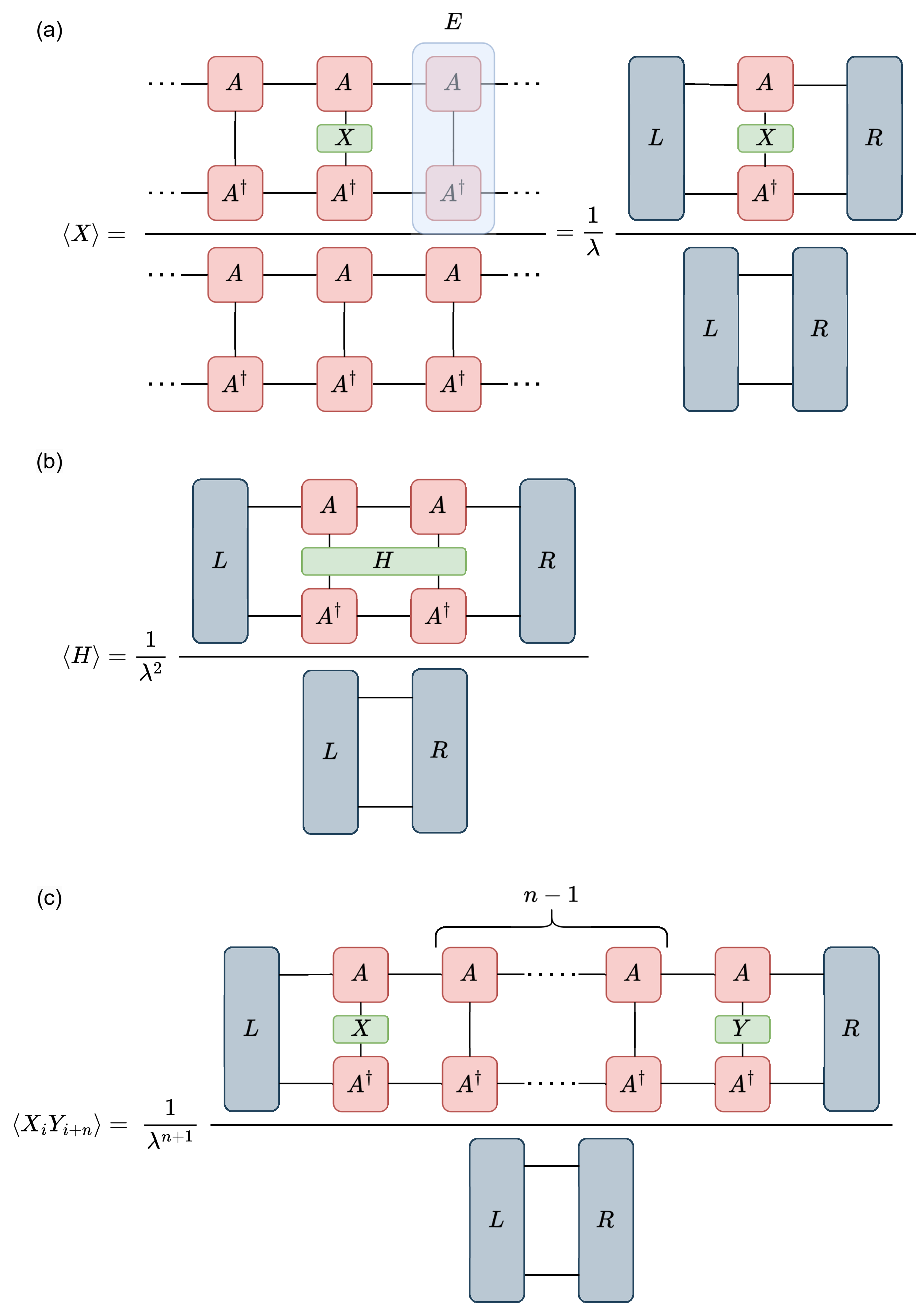
The technical details of working with MPSs have been introduced in many textbooks and review articles—for instance, see Refs. [27,28]. As is illustrated in Figure 1, the way to calculate the expected value of operators in a translation-invariant, infinite MPS involves creating the ${\chi }^2\times {\chi }^2$ transfer matrix $E={\sum }_s{A}^s\otimes A^{s†}$, and determining its leading left and right eigenvectors (L and R):

$$\begin{array}{c}\hfill LE=\lambda L;\end{array}$$

(7)

$$\begin{array}{c}\hfill ER=\lambda R.\end{array}$$

(8)

Also, the two-, three-, and four-index tensors are contracted, as seen in Figure 1. The loss function to be minimized in this case is the bond energy, which is the expectation value of the two-site Hamiltonian in the ground state:

$$\langle H\rangle ={\displaystyle \frac{L{F}^{\alpha {\alpha }^{\prime }}{F}^{\beta {\beta }^{\prime }}{H}_{\left(\alpha \beta \right)\left({\alpha }^{\prime }{\beta }^{\prime }\right)}R}{{\lambda }^{2}LR}},\mathrm{with}{F}^{\alpha \beta }=A^{\alpha }\otimes A^{\beta },$$

(9)

For more details on calculating expectation values in MPS, see [27,28].

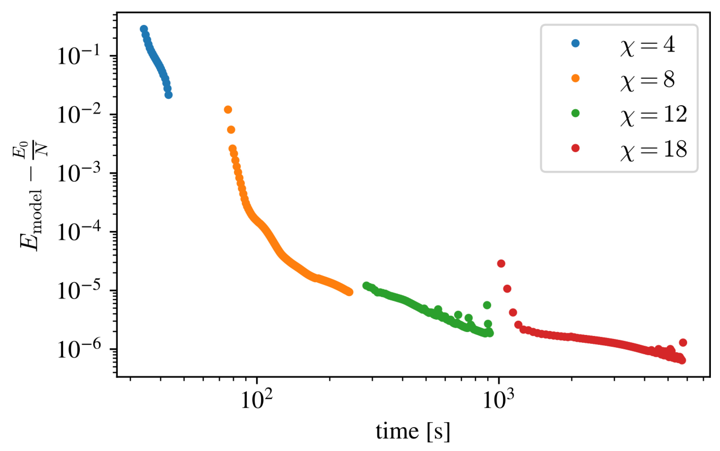
Our gradient descent optimization was performed in Python (version 3.11.7) with the ADAM optimizer [29] in TensorFlow (version 2.17.0) [30] on an NVIDIA V100 GPU. We found it beneficial to gradually increase the bond dimension $\chi$ during the algorithm; this was found to converge faster than immediately training the model with the maximum bond dimension from the beginning. We start with a small bond dimension, e.g., ${\chi }_0=4$, and optimize this small model for a few hundred epochs. We then increase the degrees of freedom to ${\chi }_1$ by combining the already trained smaller block ${\chi }_0$ and a fresh, empty block $\delta \chi$ placed along the diagonal of a larger tensor. Off-diagonal blocks are initialized with small random elements. We retrain this larger model over a few hundred cycles again. Performing this repeatedly, we can end up with an optimized MPS with a bond dimension of $\chi ={\chi }_{max}$. In Figure 2, we present an example of the training process.

The MPS determined this way is not unique. The quantum system has a gauge symmetry, but any solution minimizing the Hamiltonian provides identical results for the physical characteristics of the ground state [28].

4. Sampling from an MPS

The MPS defines a linear combination of classical spin configurations. In the ITF case, all coefficients (amplitudes) are real numbers. The square of an amplitude gives the probability that in a quantum measurement, the quantum state collapses into that particular classical configuration. As defined and determined above, this construction has no time direction. To map our quantum chain on a classical stochastic time series model, we need a sequential generation method that can build a probabilistic spin configuration one by one, starting at the leftmost point and proceeding to the right. The buildup procedure should respect the likelihoods dictated by the quantum state amplitudes.

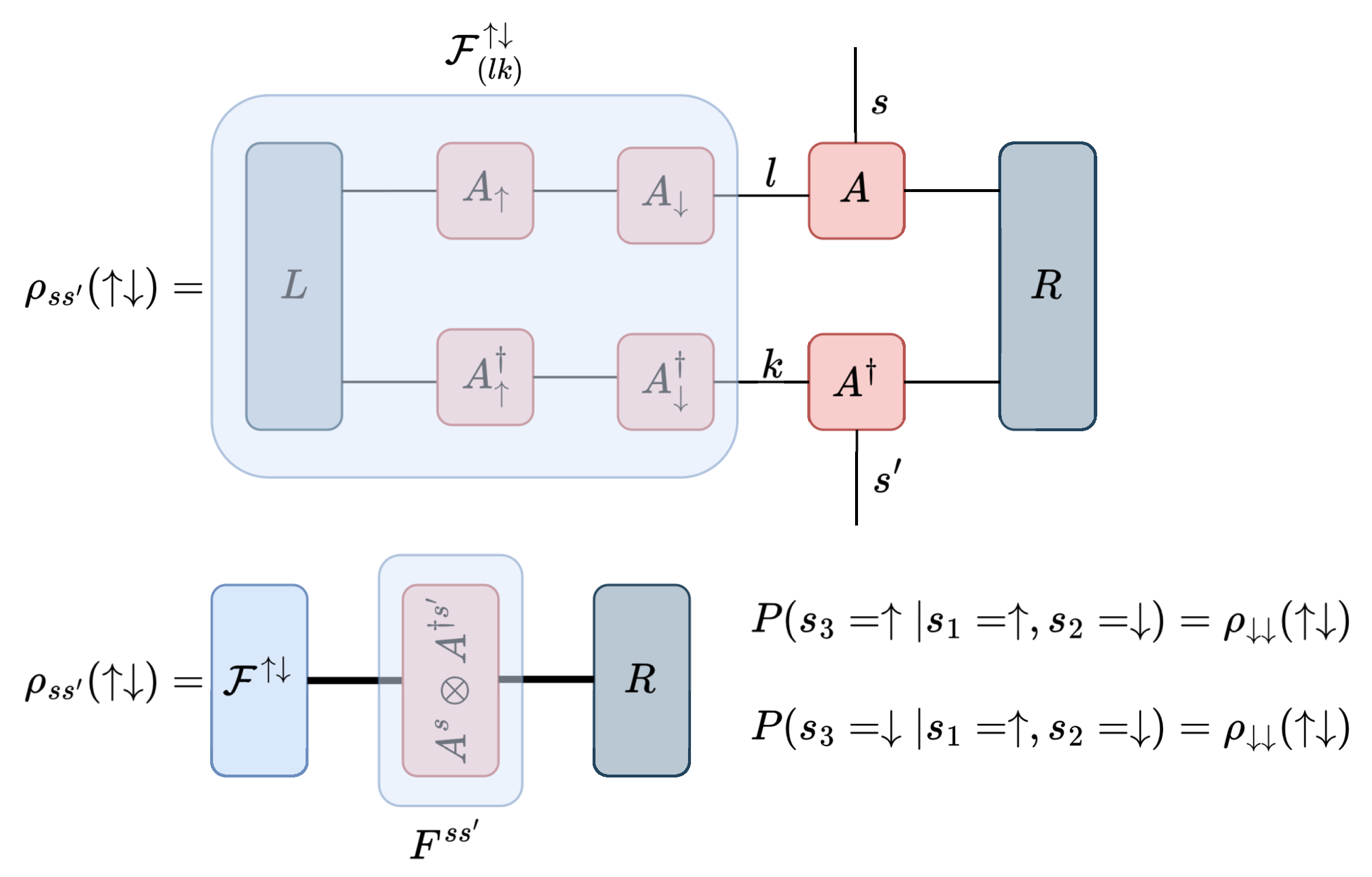
Serial sampling from a finite unitary MPS was worked out by Ferris and Vidal [31]. Their method is based on calculating single-site density matrices conditioned on earlier fixed spins (spin string) in the chain. We extended their technique to arbitrary infinite MPSs. The procedure is shown in graphical form for the third step in Figure 3 and is described below.

Assuming that the first n spins in the chain have already been sampled and take the values ${\alpha }_1,{\alpha }_2,\dots ,{\alpha }_n$, the conditional density matrix of the next spin for a general infinite chain has a simple form:

$${\rho }_{\alpha \beta }\left(\{{\alpha }_1,\dots ,{\alpha }_n\}\right)={\displaystyle \frac{1}{\mathcal{N}}}{\mathrm{String}}^{{\alpha }_1\dots {\alpha }_n}{F}^{\alpha \beta }R,$$

(10)

where $\mathcal{N}$ is a normalization factor so that $\mathrm{T}\mathrm{r}\rho =1$ and ${\mathrm{String}}^{{\alpha }_1\dots {\alpha }_n}$ is a ${\chi }^2$ size vector that is easily calculated from the previous step in the calculation:

$${\mathrm{String}}^{{\alpha }_1\dots {\alpha }_n}={\mathrm{String}}^{{\alpha }_1\dots {\alpha }_{n-1}}{F}^{{\alpha }_n{\alpha }_n}$$

(11)

With this recursive relation, we can build up the $\mathrm{String}$ vector from the first step while carrying out the sampling. At the beginning, it simply takes the value of the left eigenvector of the transfer matrix:

$$\mathrm{String}=L.$$

(12)

From the conditional density matrix, the probability of the $(n+1)$-th spin being in state ${\alpha }_{n+1}$ is calculated by taking the diagonal elements:

$$P({\mathrm{s}}_{n+1}={\alpha }_{n+1}|{\mathrm{s}}_1={\alpha }_1,\dots ,{\mathrm{s}}_n={\alpha }_n)={\rho }_{{\alpha }_{n+1}{\alpha }_{n+1}}\left(\{{\alpha }_1,\dots ,{\alpha }_n\}\right)$$

(13)

The calculation involves concatenating N instances of F tensors with their physical spin index already determined by the fixed spin string. This is effectively N matrix multiplications where the matrices used take two possible values, $A^{\uparrow }$ or $A^{\downarrow }$, according to the spin string. This is seemingly an O(N) operation, but since earlier spin indices are fixed, the already calculated product can be stored and reutilized as shown in Equation (11). Thus, calculating the next conditional density matrix is an O(1) operation, independent of the current length of the string. All together, the computational cost of sampling an N-step long sequence scales as $O\left(N{\chi }^4\right)$, where the $\chi$ dependent part comes from multiplying the already sampled part $\mathrm{String}$ with $F^{\alpha \beta }$ (see (11)).

Appendix A presents details of this sample generation algorithm in a simple $\chi =2$ case.

5. Classical Time Series

5.1. Lower Level: Individual Spins

The low-level series we consider is the one defined by the spin configuration generated with the MPS sampling algorithm described above. As the MPS is translation-invariant, our spin time series will be stationary. Stationarity means that all n-point correlations are time-translation-invariant; it does not matter where we measure these correlations along the time axis.

The spin series has discrete levels, $\{\downarrow ,\uparrow \}$ (or, using other conventions, $\{-1/2,1/2\}$ or $\{0,1\}$), and it inherits the quantum correlation structure to produce nontrivial autocorrelations. These processes are usually called Generalized Bernoulli Processes (GBPs) [32,33,34,35]. The adjective “generalized” refers to the fact that the increments are not necessarily independent but can be correlated.

The continuous-time Gaussian analog of a generalized Bernoulli process is a “colored noise” (“white noise” when autocorrelation is zero, “colored noise” when autocorrelation is non-zero). These noise processes are usually used to build integrated processes like Brownian motion or fractional Brownian motion. To follow this logic, we build an integrated process from GBP in the next section.

The same MPS can be used to generate a different GBP model after the MPS has been adequately rotated. Rotation can change the basis from the spin “z” basis to the spin “x” (or spin “y”) basis. Since x-x (or y-y) correlations are different from z-z correlations in the ITF ground state, the rotated MPS will generate a classical Bernoulli series, which is statistically different.

The basis change from the “z” basis to the “x” basis can be achieved with the help of the Hadamard matrix:

$$\mathcal{H}={\displaystyle \frac{1}{\sqrt{2}}}\left[\begin{array}{cc}1& 1\\ 1& -1\end{array}\right]$$

(14)

The transformation is simply performed on the MPS matrix in the “z” basis (${\mathbf{A}}_{\mathbf{z}}$) to obtain the MPS matrix in the “x” basis (${\mathbf{A}}_{\mathbf{x}}$):

$${\mathbf{A}}_{\mathbf{x}}{ij}^k={\mathcal{H}}^{kl}{\mathbf{A}}_{\mathbf{z}}{ij}^l.$$

(15)

The transformation is obviously carried out on the physical indices of the MPS matrices, and the bond indices are left untouched.

5.2. Integrated Process: Magnetic Domains

A spin time series generated from the translation-invariant MPS is stationary. Typical financial time series like asset prices are not stationary; they are usually modeled as integrated, unit root processes. In the continuous case, for instance, (geometric) Brownian motion as a model for asset prices is built upon a stationary noise process (the daily returns).

Using our two-state GBP (spin) series as increments, we can create integrated series in various ways. The most obvious way to build an integrated series is to consider the (uniform) domain magnetization

$$M_N=\sum _{i=1}^N{s}_i.$$

(16)

If $s_i$ were uncorrelated, $M_N$ would be binomially distributed. However, autocorrelation in s makes M distributionally nontrivial. The full statistical description of M is called “full counting statistics” in the quantum spin chain literature.

The full counting statistics of the ITF domain magnetization have been studied earlier (see, e.g., [36,37]). Methods usually leverage numerical techniques for small–medium domain sizes or use asymptotic results, such as Szegő’s theorem or the Fisher–Hartwig methods, to express the probability distribution of the random variable. In most methods, it is easier to calculate the probability-generating function and use inverse Fourier transformation to obtain the probability density function (PDF). One of the most interesting questions is how the PDF scales as the domain size increases and whether the scaling function is Gaussian or shows deviations from the central limit theorem.

In the MPS representation, the probability-generating function of the domain magnetization is easy to calculate:

$$G\left(\theta \right)=\langle \psi |e^{i\theta \widehat{M}}|\psi \rangle =\langle \psi |e^{i\theta {\sum }_k{\widehat{s}}_k}|\psi \rangle =\langle \psi |\prod _{k=1}^N\left(e^{i\theta \widehat{s}}A\right)\rangle ={\displaystyle \frac{L{\left[F^{\alpha \beta }{\left(e^{i\theta \sigma /2}\right)}_{\alpha \beta }\right]}^{N}R}{{\lambda }^{N}LR}},$$

(17)

where $\widehat{s}={\displaystyle \frac{\sigma }{2}}$ is the spin operator, and $\sigma$ can be any of the Pauli matrices. We can think of this as applying a rotation around the spin axis with angle $\theta$ on all of the MPS matrices before calculating the inner product.

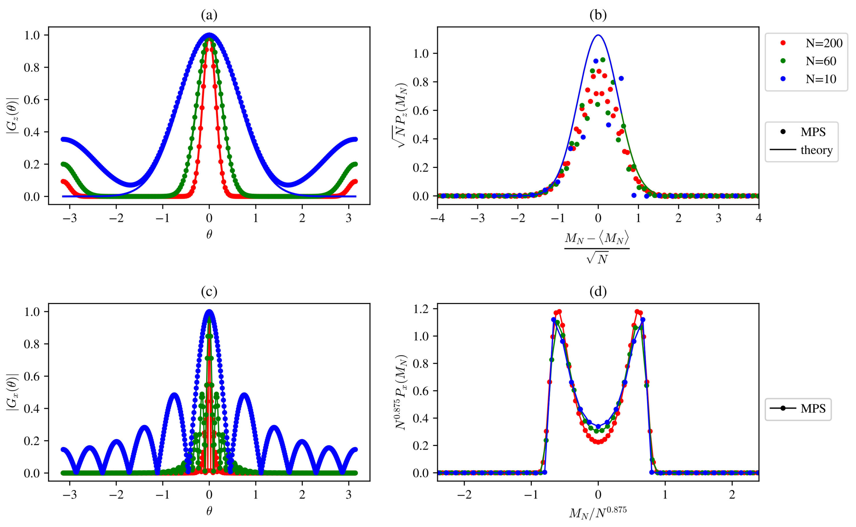
For the ITF model, earlier results show [36] that domain magnetization converges to a Gaussian distribution away from the critical point. This remains true at the critical point for the z-direction, but in the x-direction, the scaling function retains a double-peaked shape. Our MPS calculation confirms these results.

Figure 4a,b shows the unscaled generator function and scaled PDF in the z-direction. The curves calculated numerically from the MPS state follow closely the following theoretical Gaussian result:

$$G_{\mathrm{exact}}^z\left(\theta \right)=e^{i\theta \langle M\rangle -N{\sigma }^2{\theta }^2/2}.$$

(18)

with $\langle M\rangle =N/\pi$ and ${\sigma }^2=1/4$ [36]. The only noticeable deviation is at the low and high $\theta$ boundaries of the generator, resulting in a high-frequency error in the probability distribution. This is a finite-size effect that diminishes with larger domain sizes (N).

For the x-direction, only numerical results are available [36,38], again our calculation depicting a double-peaked probability distribution nicely agrees with earlier findings (see Figure 4c,d). The scaling is achieved with the standard deviation of the distribution that scales with the system size as $N^{\frac{7}{8}}$.

These results show that a discrete time series generated from the ground state of the quantum ITF model can have nontrivial statistical properties on the integrated level. The deviation from Gaussian scaling is a hallmark of quantum criticality, and the MPS representation of a time series is capable of grasping this feature when it is present.

6. Testing Ergodicity and Statistical Properties

The Hamiltonian of the ITF model is translation-invariant. The quantum ground state and the MPS approximations to this ground state reflect this translational symmetry. The model has no spontaneous breaking of this symmetry. Thus, one- and two-point expectations can be calculated by fixing the location of the operators arbitrarily along the infinite chain and calculating expected values as “ensemble averages” over the quantum superposition.

In the equivalent time series model, we do not have the complete quantum superposition at our disposal but only a random sample from this state. However, our series is (at least asymptotically) stationary, and we can generate a long enough sample and calculate expected values in a “time average” way by moving along the chain. If the system is ergodic, these two calculations are equivalent.

The time average calculation, however, limits the space of operators that can be studied. We can only work with operators that stay within the physical spin basis ($S^z$ basis) chosen originally. We can calculate $M=\langle S^z\rangle$ and $C^z\left(r\right)=\langle S_0^z{S}_r^z\rangle$, but we cannot calculate transverse operator expectations like $C^x\left(r\right)=\langle S_0^x{S}_r^x\rangle$ because they leave the restricted Hilbert space we simulate. To check these transverse correlators, we need to perform a suitable rotation of the MPS tensors first (move to an $S^x$ basis), simulate the classical configuration in this rotated space, and then calculate the space-invariant expectations.

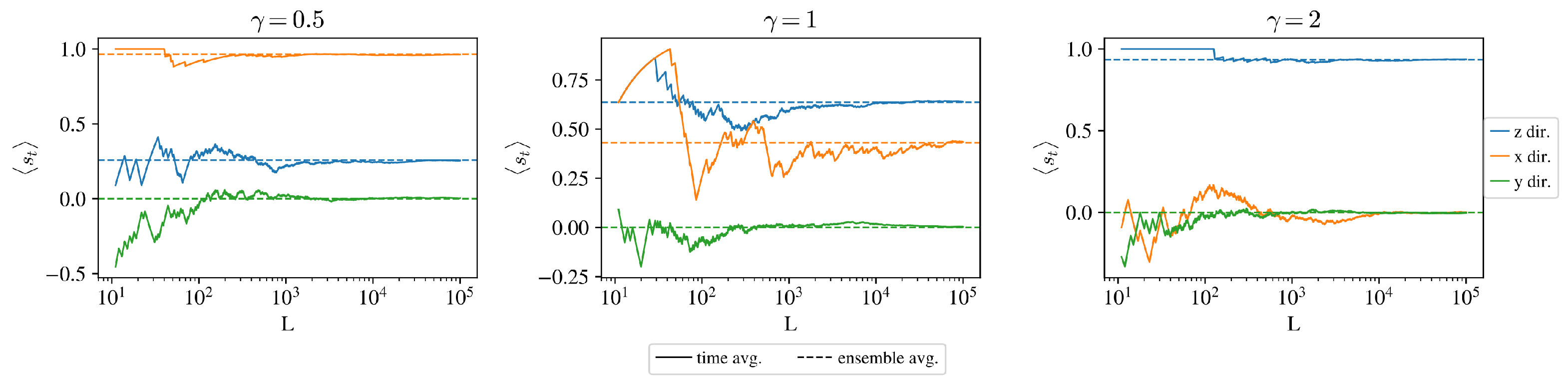
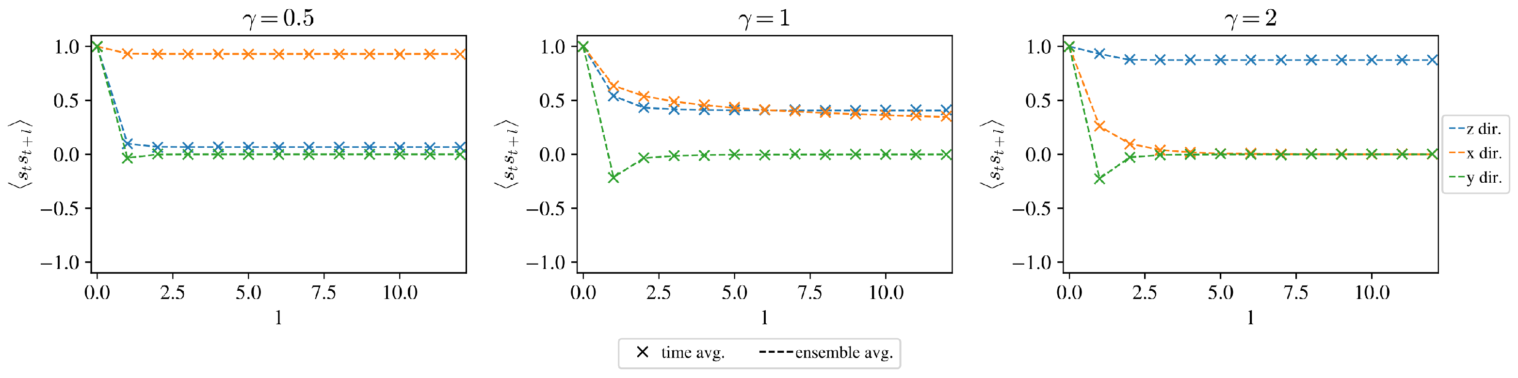
To check ergodicity, we have generated a long random sample from the numerically determined MPSs (see Section 3) and calculated $M=\langle S^z\rangle >$ and $C^z\left(r\right)=\langle S_0^z{S}_r^z\rangle$ expectations both as ensemble and time averages. Figure 5 shows how the time average converges to the quantum ensemble average. Figure 6 shows a good agreement between the time average and ensemble average correlation for a sufficiently long sample.

7. Calibrating MPS to Empirical Time Series

The MPS representation of the time series is a parametric representation in which the parameters can be calibrated to empirical data. In this section, we discuss two experiments: one on synthetic data and one on real data. A previous study has shown how an MPS can be used as a generative model for spatial, image-like data [14]; here, we focus on time series with directional causality.

Causality implies that our generative model should use past observations as input and produce the probability of the next element as output. When the autocorrelation length is finite, a reasonable approximation is to assume a higher-order Markov chain with a finite memory of length m that matches the correlation length. In a discrete model with d states, this assumes specifying a transition function that maps from $d^m$ states to $d-1$ (independent) probabilities. Altogether, these are $d^m(d-1)$ model parameters, but there are implicit constraints and relationships within these parameters. The MPS representation does a similar thing but finds an optimal, lower-dimensional representation for this finite-memory transfer function.

As an alternative to the Markov chain parametrization, we can focus on the occurrences of $m+1$-long configuration segments and record their occurrence probabilities. Empirically, this can be measured by a moving time window of size m. This representation is fully equivalent to specifying the m-th order Markovian transitional probabilities in the stationary case.

Some earlier works calibrated MPS matrices to one-dimensional patterns using a maximum likelihood approach for generative learning tasks [14,17]. In maximum likelihood, we iterate through the whole sequence, calculate the likelihood and its derivatives with respect to the parameters, and apply gradient learning. This method scales with the length of the time series observation and becomes very tedious for long series. In contrast, calibration methods working on Markovian transition probabilities or configuration probabilities of length m [16,18] do not scale with the total length of the series. Note, however, that finite memory calibration cannot capture correlations longer than the memory length m explicitly assumed.

7.1. Simple Pattern Learning

In the first synthetic calibration experiment, we created binary time series from short, repeating patterns of length m. For such series, an $(m-1)$-order Markov model would be exact and would predict the next element with certainty. We wanted to see how well an MPS model with bond dimension $\chi$ can perform in this situation. Once a long sequence was generated, we calculated the target configuration probability ${\widehat{P}}^{\left(m\right)}$ and used this in a calibration by minimizing the Kullback–Leibler (KL) divergence of ${\widehat{P}}^{\left(m\right)}$ and the MPS ($\chi$) model implied configuration probability distribution $P^{\left(m\right)}$.

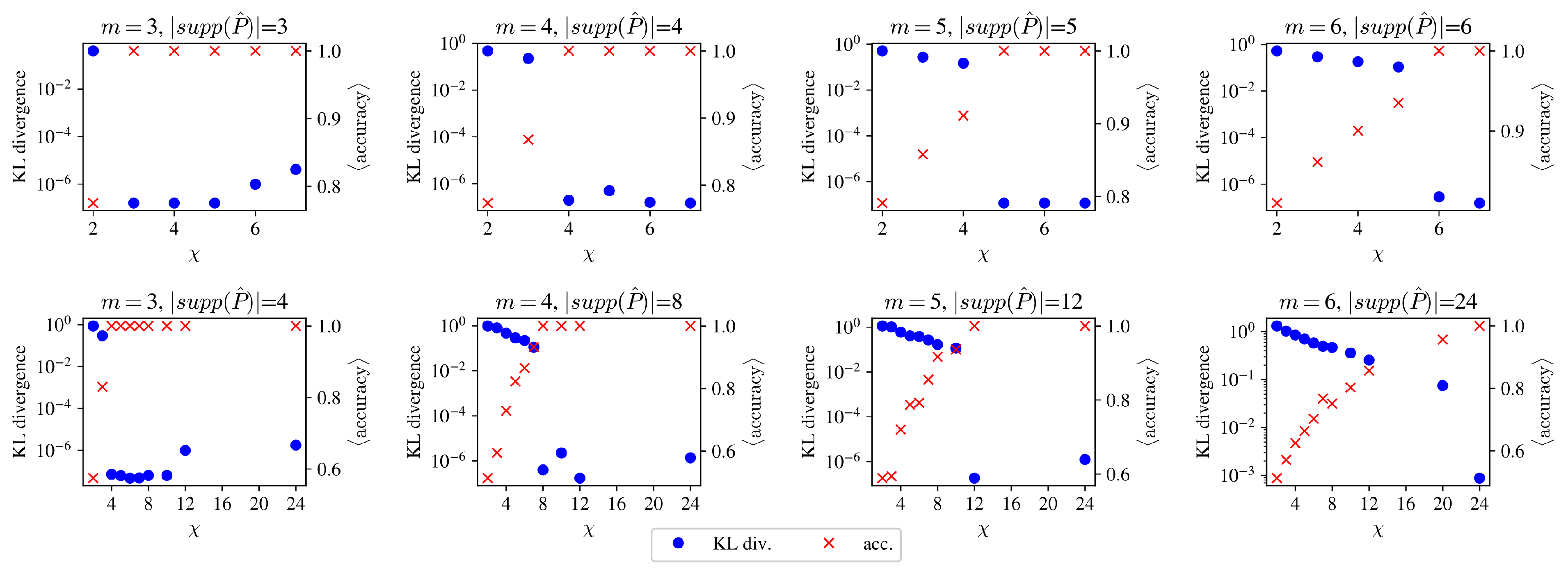
Figure 7 shows how a fully trained MPS model performs as a function of the bond dimension $\chi$. We find that it is not the memory length m or the bare size of the configuration space $2^m$ that determines the necessary MPS bond dimension for good calibration, but the size of the “support”, i.e., the number of non-zero elements in ${\widehat{P}}^{\left(m\right)}$. As can be seen in Figure 7, there is a sudden increase in accuracy (drop in KL divergence) in all cases when the bond dimension reaches the size of the support of the configuration probability distribution. Based on this, we can say that an MPS can represent a configuration probability distribution almost perfectly if $\chi >\left|\mathrm{supp}\right(\widehat{P}\left)\right|$.

Note that this is a weak result, as for a general time series, $\mathrm{supp}\left({\widehat{P}}^{\left(m\right)}\right)\sim 2^m$. However, the following experiment shows that support-based scaling might be the worst-case scenario for an MPS.

7.2. Air Pollution Data

In this section, we will show how an MPS can be trained for a real stochastic time series. As our empirical time series, we work with air pollution data for Seoul city downloaded from Kaggle (hourly air pollution data for Seoul city Seocho-gu district between 2017 and 2019 provided by the Seoul Metropolitan City; https://www.kaggle.com/datasets/bappekim/air-pollution-in-seoul/data; accessed on 18 December 2024). We discarded measurement points when instrument status was “abnormal”, “power cut off”, “under repair”, and “abnormal data” and ended up with 24,748 data points. The dataset was chosen because setting a proper threshold limit (we use a value of $50{\mathrm{\mu /m}}^3$ according to the WHO for PM10 measurements) provides an easy binarization of the time series, as previously carried out in Ref. [39].

7.2.1. Kullback–Leibler Divergence-Based Optimization

First, to compare the training on the real and artificial data of the previous section and to support the claim that training on exact patterns is harder than on the real data, we performed a similar training by optimizing the KL divergence between the ${\widehat{P}}^{\left(m\right)}$ of the data and $P^{\left(m\right)}$ of the MPS representation. We set a memory length of $m=6$ for calibration—i.e., we work with ${\widehat{P}}^{\left(6\right)}$. 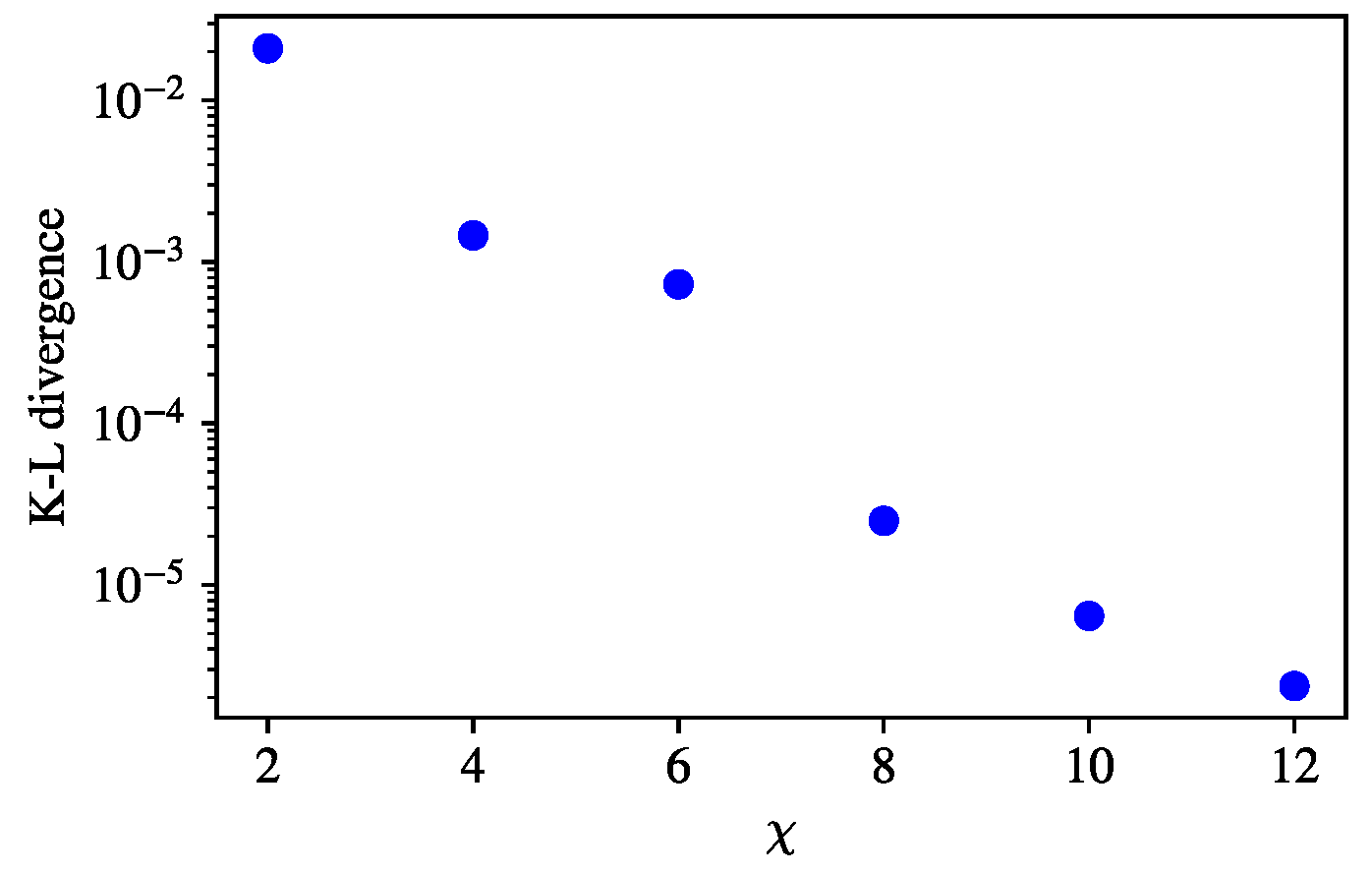We can see in Figure 8 that already for $\chi =6$ the KL divergence reaches ${10}^{-3}$, even though $\left|\mathrm{supp}\right({\widehat{P}}^{\left(6\right)}\left)\right|=64$. This could have only been possible for $\chi =64$ in the pattern learning case for ${\widehat{P}}^{\left(6\right)}$ with $\left|\mathrm{supp}\right(P^{\left(6\right)}\left)\right|=64$. We note that the convergence slowed down, meaning that the complex probability distribution is harder to learn but easier to represent for the MPS representation.

7.2.2. Calibration to the Correlation Function

For a stochastic process, the predictive accuracy used in the previous section is usually not a good metric for the goodness of the representation, as it may be inherently unpredictable or predictable with low accuracy. For example, think of a random sequence. For this reason, we will compare the two-point correlation between the MPS representation and the series and the KL divergence. These are meaningful comparisons for generative usage and for predictive models as well.

Training the MPS to match the distribution ${\widehat{P}}^{\left(m\right)}$ of the sequence is hardly reasonable for practical applications since the already obtained ${\widehat{P}}^{\left(m\right)}$ can be used at least as well for sample generation as the MPS trained on it. A slight advantage could be possible memory-saving by discarding the ${\widehat{P}}^{\left(m\right)}$ vector and retaining only the potentially smaller MPS matrices. The MPS matrix may have a lower number of parameters because the MPS representation can achieve a correlation length that scales as ${\chi }^{\kappa }$ with the bond dimension. A previous study found $\kappa$ to be $1.37$ and 2 for two cases [40], whereas the distribution ${\widehat{P}}^{\left(m\right)}$ has a correlation length of m that is easily seen because it has no information beyond the distance m. If we include the number of parameters for the representations, that is,

$$\begin{array}{ccc}\hfill {\#}_{MP{S}_{\chi }}& =& 2{\chi }^2\hfill \end{array}$$

(19)

$$\begin{array}{ccc}\hfill {\#}_{{\widehat{P}}^{\left(m\right)}}& =& 2^m,\hfill \end{array}$$

(20)

we can compare the correlation length to the number of parameters:

$$\begin{array}{ccc}\hfill {\xi }_{\mathrm{MPS}}& \propto & {\left({\#}_{MPS}\right)}^{\kappa /2}\hfill \end{array}$$

(21)

$$\begin{array}{ccc}\hfill {\xi }_{P^{\left(m\right)}}& \propto & {log}_2\left({\#}_{P^{\left(m\right)}}\right).\hfill \end{array}$$

(22)

We can see that a large MPS representation may have a substantial advantage in capturing long-distance correlations over the configuration probability distribution.

To exploit the longer (auto-)correlation length and demonstrate the advantage of the MPS representation, we defined a loss function that explicitly calibrates to the observed correlation values up to some cut-off distance $r_{\max }$:

$$L_c^{\left(r_{\max }\right)}=\sqrt{{({\langle x_t\rangle }_{\mathrm{MPS}}-{\langle x_t\rangle }_{\mathrm{obs}.})}^2+\sum _{r=1}^{r_{\max }}{[C_{\mathrm{MPS}}\left(r\right)-C_{\mathrm{obs}.}\left(r\right)]}^2},$$

(23)

where $C_{\mathrm{MPS}}\left(r\right)$ is the correlation function calculated directly from the MPS matrix as described graphically earlier in Figure 1. For this concrete calculation $X=Y=S_z$, ${\langle x_t\rangle }_{\mathrm{MPS}}$ and ${\langle x_t\rangle }_{\mathrm{obs}.}$ are the expectation value of the MPS and the average of the time series, respectively.

This is practically equivalent to calibrating the whole ${\widehat{P}}^{\left(m\right)}$ distribution, as the expectation value and the two-point correlations up to length m determine the entire $P^{\left(m\right)}$ distribution uniquely for stationary binary time series. However, with this loss function, we completely avoid calculating and storing the $2^m$ elements of $P^{\left(m\right)}$.

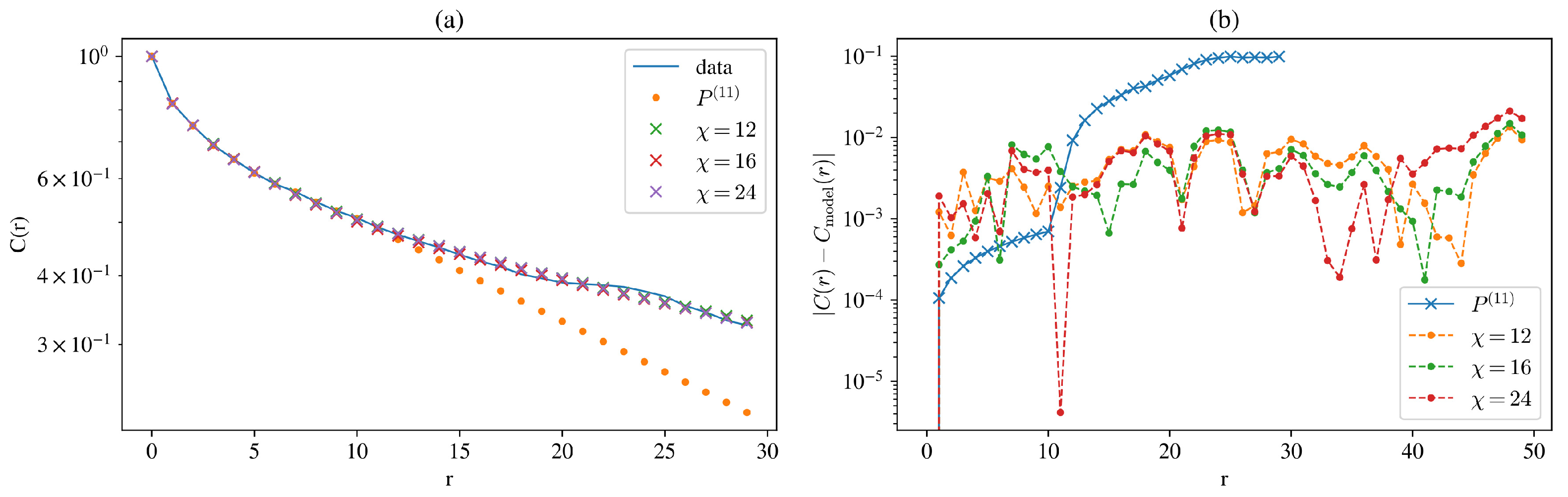
We trained MPS matrices with different bond dimensions on the loss function $L_c^{\left(30\right)}$, which considers correlations up to $r_{\max }=30$. Our results show that the MPS representation has, indeed, the ability to represent long-range correlation with fewer parameters than the configurational probability distribution. In Figure 9a, we can see that the air pollution data have a slowly decaying autocorrelation, and the calculated correlation based on the distribution ${\widehat{P}}^{\left(m\right)}$ loses precision rapidly at length m, whereas ${\mathrm{MPS}}_{\chi }$ performs better for longer distances. Figure 9b plots the representation error. Note that up to length m, distribution-based correlations should be without error; the only caveat is the edge effect that makes the distribution lose perfect translational invariance. Above $m=11$, they increase rapidly.

The error of the MPS correlations stays below $1\%$ up to a distance of 40, even outside the training correlation length. This is certainly only possible if the correlation has a smooth decay since the MPS representation has no information on correlations beyond 30 time steps.

Importantly, the distribution ${\widehat{P}}^{\left(11\right)}$ considered in this experiment has $2^{11}=2048$ parameters, while the MPS representations with bond dimensions $\chi =12,16,24$ have only $288,512$ and 1152 parameters, respectively.

8. Discussion

In this paper, we looked into an intriguing analogy between quantum spin chains and classical binary time series. In the quantum context, classical configurations arise naturally as the result of measurements on the wavefunction of the system. The probability and the statistical properties of the configurations generated by such measurements are highly influenced by the nontrivial dependency structure within the quantum state.

The dependency structure of the wavefunction can be approximated by a matrix product state (MPS) Ansatz. This representation is optimal in terms of compression; it approximates the wavefunction with high precision and a minimal number of calibration parameters. Also, a number of statistical metrics can be calculated from an MPS with minimal effort.

We demonstrated that the MPS Ansatz for the classical time series is a meaningful model. It is capable of generating samples sequentially with linear cost, which is an important requirement dictated by the causal structure of time series. When the MPS is translation-invariant, both the quantum state and the classical time series derived from it are also translation-invariant. Determining quantum correlations by ensemble averaging becomes equivalent to determining autocorrelations by time averaging. Results obtained for the quantum problem can be directly transferred to the equivalent classical time series.

We looked into several methods for calibrating an MPS model to an empirical time series. The computational cost of the likelihood-based training impelled us to use other methods, such as one based on precalculating the Markovian transition matrix up to a certain distance and using that as a reference point for error definition in training. This makes calibration scale with this Markovian memory length and not the chain length. A similar alternative is to calculate empirical autocorrelations and try to match these through gradient descent. We found that this latter method is particularly successful in calibrating an MPS to a time series with long-range correlations.

Our study demonstrates that even a translationally invariant MPS representation with only one $\chi \times \chi$ size MPS matrix can be trained to match transition probabilities and autocorrelation functions. We showed that not all transition probability matrices are equally hard to represent—or at least train—in this formalism, with less natural sparse distribution found to be more challenging.

Given that the scale-invariant ground state of quantum spin chains at the critical point maps into a classical time series representing super-diffusion with anomalous Hurst exponents and non-Gaussian limit distributions, we expect the spin chain representation to be particularly useful for modeling time series with such properties. This can be a use case for future quantum computers. In spite of this, the MPS is not a natural representation of spin chains close to the critical point. The $O\left(N\right)$ scaling of sampling holds, but the size of the MPS matrices required to maintain a selected precision grows to infinity at the critical point.

The computational cost of the calibration and sampling process is greatly influenced by the bond dimension $\chi$ of the MPS matrix, as the algorithms involve multiplying by ${\chi }^2\times {\chi }^2$ matrices. Further investigation may be necessary to determine the required bond dimension for adequate precision.

In the paper, we used the example of a two-state quantum chain, but we can map multi-state quantum chains to multi-state classical time series in a similar vein. Practical applications on continuous problems may require a discretization of the state variable, but this is a standard engineering compromise that can be easily implemented in many practical problems. Our current approach can only model stationary and difference-stationary time series, but with a non-translationally invariant, i.e., a site-dependent MPS Ansatz, this constraint can be lifted at the expense of additional complexity. We leave these extensions for further studies.

We limited our study to MPS Ansatz-based models and a few calibration metrics, but other types of tensor networks and loss functions may prove useful for modeling slow decaying correlation. Future research should determine the advantages of the proposed framework against other classical techniques as well as other calibration methods.