Abstract
Waste heat recovery is a critical strategy for optimizing energy consumption and reducing greenhouse gas emissions. In this context, the circular economy highlights the importance of this practice as a key tool to enhance energy efficiency, minimize waste, and decrease environmental impact. Artificial neural networks are particularly well-suited for managing nonlinearities and complex interactions among multiple variables, making them ideal for controlling a double-stage absorption heat transformer. This study aims to simultaneously optimize both user-defined parameters. Levenberg–Marquardt and scaled conjugated gradient algorithms were compared from five to twenty-five neurons to determine the optimal operating conditions while the coefficient of performance and the gross temperature lift were simultaneously maximized. The methodology includes R2024a MATLAB© programming, real-time data acquisition, visual engineering environment software, and flow control hardware. The results show that applying the Levenberg–Marquardt algorithm resulted in an increase in the correlation coefficient (R) at 20 neurons, improving the thermodynamic performance and enabling greater energy recovery from waste heat.
1. Introduction
Waste heat recovery has established itself as an essential strategy to optimize energy consumption and mitigate greenhouse gas emissions in industry [1]. In parallel, the use of renewable energy continues to grow rapidly, and it is projected that by the end of 2025, it will account for approximately 30% of global energy consumption [2]. In this context, absorption heat transformers (AHTs), considered a type of absorption heat pump [3], stand out as thermodynamically efficient equipment, capable of adapting to renewable sources such as solar and geothermal [4] and converting waste energy into a valuable resource, boosting sustainability and industrial efficiency [5,6].
The circular economy promotes waste heat recovery as a fundamental practice to optimize energy use, minimize waste, and reduce the environmental impact of industrial processes [7]. The integration of absorption heat pumps, with circular economy principles, is becoming increasingly important to improve energy efficiency and reduce environmental impacts in various industrial sectors. Recent studies highlight the central role of absorption heat pumps in the recovery and reuse of waste heat, as well as in the efficient conversion of energy resources supporting the circular economy model [8,9]. These applications encourage the reuse of resources and reduce dependence on primary sources.
In addition, research on efficient cogeneration systems [10] and latent heat recovery technologies in wet biomass flows [11] underlines the importance of absorption heat pumps to close energy cycles in industrial processes. Likewise, the integration of renewable energies, such as concentrated solar power for low-pressure steam generation [12], or the optimization of hydrogen-integrated energy centers [13], reinforces the transition to sustainable models, demonstrating that AHT can be a key catalyst for the synergy between energy efficiency and economic sustainability.
Due to the multiple variables present in the thermodynamic cycle of an AHT, the need arises for an automatic control that considers in its strategy both the multiple variables present in the cycle as well as the associated disturbances that can guarantee its correct operation. Proposals for automatic control related to classical control methods, such as PID (proportional–integral–derivative) controllers, have been published in the literature [14]; however, these approaches are limited to nonlinear and multivariable systems such as AHTs. This study was limited to calculating the flow ratio; however, the control response in the two cycles was not characterized.
On the other hand, artificial intelligence (AI) technologies, such as artificial neural networks (ANNs) and fuzzy logic (FL), have become key tools for the development of advanced control systems. These methodologies stand out for their ability to efficiently manage nonlinearities, multivariable interactions, and uncertainty scenarios, making them ideal for applications in complex and dynamic systems [15].
Several scientific publications have reported the use of ANN applied to thermal processes. Ref. [16] uses ANN in heat pumps to improve demand response, achieving high precision and optimizing energy consumption. Ref. [17] apply reinforcement learning to optimize control in a heat pump, achieving greater efficiency in energy management. Ref. [18] uses ANN to control a heat pump to improve energy efficiency and thermal comfort. Sajadi predicts real-time temperature fields in manufacturing processes using ANN [19]. In addition, Yarahmadi proposes the ANN in a laser powder bed fusion process to predict the distribution of the temperatures present [20]. On the other hand, in pyrolysis processes, Muravyev focuses on the application of ANN for thermal analysis [21]. Also, Zhang combines ANN and genetic algorithms to maximize heat transfer and minimize pressure loss of finned heat exchangers with elliptical tubes [22], but there is no ANN for a double-stage absorption heat transformer (DSHT) for maximizing simultaneously coefficient of performance (COP) and gross temperature lift (GTL).
This study is based on the premise that no reports in the literature on applications of double-stage absorption heat transformers that use artificial intelligence for automatic control. This system presents multiple variables with high nonlinearity, such as enthalpy, which are essential for the calculation of the thermal power of the eight heat exchangers that make up the thermodynamic cycle. Furthermore, the double-stage absorption heat transformer requires centralized automatic control that considers all the present variables and the associated disturbances. The measured data can be trained by artificial neural networks, allowing for greater accuracy compared to previously published idealized models [6].
The objective of this work is the fusion of the technology of R2024a ANN-Matlab© software with a commercial mass flow control system to obtain the maximum value of the temperature desired by the user simultaneously with the maximum value of the performance coefficient as a function of the surrounding temperatures (condenser temperature in AHT (TCO) associated with that of the environment, generator temperature in AHT (TGE) associated with the temperatures of the waste heat source) for circular economy thermal processes. This work is a continuation of our previous publication [3], in which only the control strategy based on maximizing the COP × GTL product separately for each stage of the AHT was presented.
2. Materials and Methods
This section identifies the software, hardware, and flowchart used for fluid flow control (MEV1), as well as the methodology used to obtain the maximize the COP × GTL using artificial intelligence techniques.
2.1. Signal Characterization
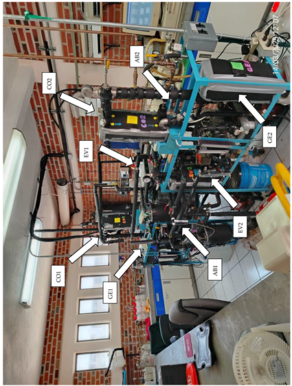
A computer-aided simulator was developed based on experimental data obtained in the prototype of the double stage heat transformer (DSHT) physically installed in the Laboratory of Applied Thermal Engineering of the Center for Research in Engineering and Applied Sciences (CIICAP) of the Autonomous University of the State of Morelos, Mexico. Based on experimental data, this simulator was developed with the main objective of analyzing the system’s behavior under different operating conditions. Additionally, it determines the time required to reach a desired state from the transient heating stages. In Appendix C, an actual photograph of the DSHT is shown on the entire page.
To this end, in each test, the temperature variations during the heating stage were recorded and the coefficients of the function that presented the highest correlation in each case were obtained. These coefficients, together with temperature variations, allowed the generation of a third-degree polynomial function that describes the variation in temperature over time. This tool enables the analysis of temperature behavior in each DSHT channel at any given time. Table 1 and Table 2 present the 44 temperature channels of the equipment and the functions obtained for each of them. Additional uncertainty analysis was calculated for each temperature channel at operating conditions of each by error propagation theory.

Table 1.
DSHT stage 1 channel temperature variation function.
Table 2.
DSHT stage 2 channel temperature variation function.
2.2. Artificial Neural Networks
The control strategy applied to operate the DSHT under conditions that maximize the COP × GTL product is based on determining the first stage working fluid flow value (MEV1) using MLP-ANN [3]. The developed ANN consists of 9 input variables and 9 output variables forming a MIMO (multiple-input and multiple-output) system. The names and units of measurement of inputs and outputs are shown in Table 3. See Appendix C to identify from right to left in the photograph of the laboratory’s prototype, the condenser 1 (CO1 label), generator 1 (GE1 label), evaporator 1 (EV1 label), absorber 1 (AB1 label), condenser 2 (CO2 label), generator 2 (GE2), absorber 2 (AB2) and evaporator 2 (EV2 label).
Table 3.
Input and output variables of the ANN model.
The range of the input variables is adjusted to the operating conditions evaluated for the DSHT, with a variation of 1 °C. Although the absorber in AHT (AB1) provides a higher thermal level available for the evaporator in DSHT (EV2), EV2 operates at the equilibrium temperature required for the concentration feed of the Stage 2 system. Any excess energy supplied by AB1 to EV2 results in increased pressure. The output variables were normalized within the range of 0.0 to 1.0 and the accuracy is reported. The range of these values is presented in Table 4 which has 10 input variables and 10 output variables, making it a MIMO system (multiple input–multiple output).
Table 4.
Variables and values of input and output variables.
The neural network learning algorithm adjusts the weights and biases to obtain the desired outputs minimizing the error [23]. There is no single method to determine the optimal number of neurons or layers in the network, so a trial-and-error approach is employed [24]. In this study, the number of neurons in the hidden layer was established by ensuring that the correlation between the output generated by the network and the expected values was greater than 0.9998.
The ANN was programmed using the MATLAB © nftool (Neural Fitting) tool that facilitates data selection, the creation and training of neural networks, as well as the evaluation of their performance by calculating mean square error and regression analysis [25]. Several networks with different neurons in the hidden layer were tested, ranging from 5 to 25. To train the networks, the data were randomly divided into three sets as follows: 70% was used for training, 15% was used for validation, and the remaining 15% was used as a completely independent test of the generalizability of the network [3].
The MATLAB© toolbox (nftool) allows you to develop an artificial neural network (ANN) with a predetermined feedforward architecture, in which the number of neurons in the hidden layer can be adjusted. To evaluate the model’s performance during the training, validation, and testing phases, the toolbox uses metrics such as the correlation coefficient (R) and the mean square error (MSE).
During ANN training, a mechanism called validation checks (early stopping) is used to monitor the validation error. Its function is to stop training when the validation error begins to increase after several iterations, thus avoiding overfitting and improving the model’s generalization capabilities.
Appendix A (Figure A1) presents a flowchart explaining how the number of neurons in the ANN hidden layer is determined, following the criterion of maximizing R. The process begins in MATLAB’s nftool, where the input and output data are first imported. The nftool randomly determines 70% of the data for training, and the user defines the percentage for validation and testing, in our case 15% for each. Next, the number of neurons (N) in the ANN hidden layer is initialized. After training the ANN, the R values (training, validation, and testing) are obtained, and these data are saved in Excel.
The number of neurons is then increased, and the network is retrained to calculate the new R values (training, validation, and testing), and these data are saved again. If the current values of R (training, validation, and test) are greater than the previous ones, the number of neurons in the hidden layer is increased again. This process is repeated until the current values of R (training, validation, and test) no longer exceed the previous values of R (training, validation, and test), at which point the cycle ends, obtaining the neurons needed to configure the ANN and completing the cycle.
Two optimization algorithms for ANN training were tested: the Levenberg–Marquardt method (LM) and the scaled conjugate gradient (SCG). According to [26], the LM method is accurate, but computationally expensive, especially for large networks. On the other hand, the SCG method is faster, although its accuracy is lower, especially in complex networks. In this study, the LM algorithm was chosen, since even though its computation time is longer than that of SCG, this aspect is not relevant, since the DSHT operates in a steady state for long periods, requiring maximum accuracy for its control.
To ensure the reliability of this database, experimental data from the DSHT were used, with a total of 155,520 samples. Of these, randomly, 108,864 samples were used in the training phase, 23,328 values for validation, and the remaining were used for testing. Training the ANN, using both the Levenberg–Marquardt and scaled conjugate gradient algorithms, leads to the optimal point, defined as the maximum value of the product COP × GTL, allowing both maximum possible values to be achieved simultaneously for the desired condition.
2.3. Hardware and Software
2.3.1. Automatization for Flow Control
The devices were used to collect data on the variables (temperature and flow) as well as to control the MEV1 flow are shown in Figure 1. These include a Model 34970A Data Acquirer with three 34901A modules, thermocouples, a flow sensor, an Arduino UNO, a servo valve, and a computer.
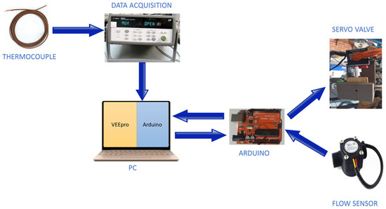
Figure 1.
Hardware implemented for signal acquisition and control of the DSHT.
For the control of the MEV1 flow of the DSHT, a 1/2-inch manual ball valve (on/off) coupled to a servo motor was used as the final control element. According to a previous study carried out by [27] the torque necessary for the opening and closing of this valve is around 1.57 Nm. It was decided to use the SAVOX SB2290SG servomotor with 4.41 Nm of torque, since this is higher than what is needed to rotate the valve, which operates with a voltage of 6 V to 7.4 V, velocity of 6 V: 0.16/60 °s and 7.4 V: 0.13/60 °s. Besides, its outstanding feature lies in its ability to receive a PWM (pulse width modulation) control signal, which facilitates the manipulation of its angular position in a simple way.
For the coupling of the servo motor to the manual valve, a piece that fits onto the top of the valve was used, in addition to another part that was 3D printed to keep the servo motor fixed; both allow the valve to adjust its rotation from 10 to 85 degrees as shown in Figure 2a.
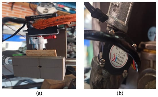
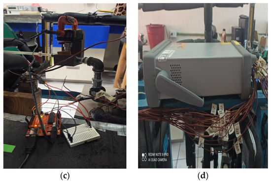
Figure 2.
This figure describes devices used in control: (a) servo valve used for MEV1 flow control; (b) flow sensor coupled to the DSHT; (c) connecting the Arduino® UNO to the flow sensor and servo valve; (d) acquisition system 34970A, 34901A modules, and thermocouples.
2.3.2. Flow Sensor
The acquisition of the DSHT MEV1 flow rate was carried out using a 1/2-inch YF-S20 flow sensor, allowing the measurement of water flow to determine consumption (Figure 2b). This sensor operates at a voltage of 4.5 V to 18 V DC, working flow rate of 1 to 30 L/min, and accuracy of ±10%. It operates thanks to the flow of water that activates a turbine connected to a magnet; when turned, this magnet activates a Hall effect sensor. The electrical impulses generated by this sensor can be interpreted by a digital input from an Arduino.
The sensor generates a square wave, with a frequency proportional to the flow rate [28]. The conversion factor from frequency (Hz) to flow rate (L/min) varies between models and depends on pressure, density, and even the flow itself, Equation (1), where Q [L/min] represents the flow, f [Hz] the frequency, and k is the conversion factor; in the case of this sensor, the average conversion factor provided by the manufacturer is 7.5.
2.3.3. Arduino® UNO Interface
The Arduino® UNO features in its configuration 14 digital input/output pins, 6 analog inputs, a 16 MHz quartz crystal, a USB connection, a power connector, and a reset button [29]. The Arduino UNO microprocessor was used, because with the digital input pins you can acquire the MEV1 digital flow signal provided by the flow sensor mentioned above. In addition, it has a PWM output that serves to send the necessary signal to the servomotor.
Figure 2c illustrates the physical connection of the Arduino to a breadboard, thus linking the flow sensor and servo valve. The 5V (Vdc) and ground (GND) pins of the Arduino are connected to the microboard using cables. The microboard, in turn, is connected to the flowmeter and the servo valve. The flowmeter data signal is linked to pin 2 of the Arduino, configured as a digital signal, while the servo valve is linked to pin 3 of the Arduino, intended for the PWM signal.
The MEV1 flux generated by the ANN, which corresponds to the maximum product of COP × GTL, represents the flux necessary for the DSHT to operate in its best scenario according to the input vector introduced in the ANN. According to [3] one of the important parameters of the DSHT is the flow ratio (FR), a dimensionless value that is calculated as the ratio between the concentration of lithium bromide in the generator and the difference in concentrations between the generator and the absorber. This value is also equal to the ratio of the dilute lithium bromide solution flow to the refrigerant flow. According to [14], a variation in concentration causes alterations in the FR, which initially impacts the flows of the evaporator and the absorber, and later those of the generator, in accordance with the conservation of matter. These changes are restricted by thermodynamic equilibrium conditions, which consider parameters such as pressure, temperature, and concentration.
The control stability under operating conditions was evaluated, and the standard deviation was 0.002245 kg/s.
The correspondence between the MEV1 flow and the opening or closing angle of the servo valve (α) is shown in Table 5, according to Equation (2). Using the R2 metric, the variations of the MEV1 flow in each test performed in the laboratory were analyzed for the variation of the rotation angle of the servo valve with a range of 10 to 85 degrees, resulting in second-degree polynomial functions. These equations correspond in each case for a unit of QAB2.
where
Table 5.
Ratio of the MEV1 flow to the opening or closing angle of the servo valve.
- M: Flow [kg/s];
- α: Servo valve angle [°C]
2.3.4. Data Acquisition
The Agilent Acquirer model 34972A was used, which supports the insertion of several modules for various functions, with a maximum capacity of three modules. In this instance, three 34901A modules were used, to which J-type thermocouples were connected. It has an operating temperature range of −210 °C to 760 °C, with a standard accuracy of ±2.2 °C or ±0.75% of the measured value. The total number of thermocouples connected to the data acquisition system is 44, representing the different physical temperatures of the DSHT (Figure 2d).
2.3.5. Visual Engineering Environment Software
For the development of the MEV1 flow control, Visual Engineering Environment (VEE) Pro-9.33 was used as the main program in parallel with the Arduino software (IDE). Appendix B (Figure A2) shows the flow diagram that begins by acquiring the temperature and absorption power provided by the user, as well as the acquisition of the data through the data acquirer. Once these data are obtained, if this condition is not met, the program ends. If the condition mentioned above is true, it means that the necessary entry vector is available to enter the ANN.
The ANN generates the necessary output values that respond to the increased product of COP × GTL, leading to the first-stage fluid flow (MEV1). This flow value is sent to the IDE software via serial port, and with the PWM signal of the same, the value of the degree of opening or closing of the corresponding servo valve is sent.
Once the servo valve varies the necessary degrees, the physical (MEV1_physical) flow value sensed by the flow sensor is acquired through the digital input of the Arduino. With this feedback, a comparison is made between the MEV1_ANN and the MEV1_physical and if the condition that they are different is met, it means two things:
- Changes in the vector of operating conditions of the DSHT.
- Acquiring the MEV1_physical value before detecting the valve rotation value.
Therefore, the program must follow this same dynamic, and if the condition is not achieved, MEV1_ANN and MEV1_physical are the same. In this condition, the program continues sending the same angle value to the valve. The iterative process continues until the input vector’s operating conditions change.
3. Results
A search was carried out to determine the value of the R greater than 0.9998 and an MSE as close to zero as possible, using the Levenberg–Marquardt method as an optimization algorithm. To do this, five to twenty-five neurons were tested in the occult layer (Table 6). The results indicate that when using 20 neurons in the hidden layer, the lowest values of MSE and the highest values of R were obtained for training, validation, and testing. Thus, the ANN was configured with 20 neurons in its hidden layer.
Table 6.
MSE and R referring to neurons present in the hidden layer of the ANN.
The ANN was designed with twenty neurons (Ns = 20) in the hidden layer (Figure 3), resulting in 180 weights, Wi{k,s} = 180 as shown in Table 7 and Wo{l,s} = 180 according to Table 8. Two bias vectors were used: one with twenty values (b1) and another with nine values (b2), detailed in Table 9. This configuration was used to predict the output values associated with the maximum product of COP × GTL, considering a vector of input conditions corresponding to the DSHT.
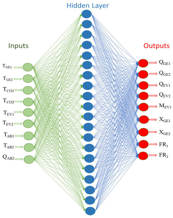
Figure 3.
Model of the neural network perceptron multilayers.
Table 7.
Weights of the input vector with respect to the hidden layer of DSHT ANN.
Table 8.
Hidden layer weights with respect to the DSHT ANN output vector.
Table 9.
Biases of the DSHT ANN model.
Using trial and error, MSE minimums of 1.78592 × 10⁻⁵, 1.97765 × 10⁻⁵, and 1.77207 × 10⁻⁵, respectively, were achieved by employing 20 neurons in the hidden layer. These low MSE values indicate optimal network performance in predicting the maximum COP × GTL output based on input operating conditions. In addition, the regression plots confirm the effectiveness of the model, showing a strong fit for all datasets with correlation values (R) greater than 0.9998 (Figure 4).
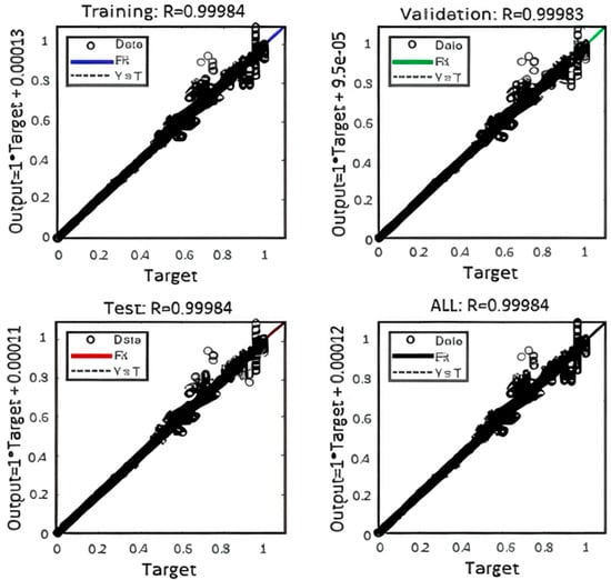
Figure 4.
Regression of the proposed ANN for DSHT.
Transient State Simulator and DSHT ANN
After the creation of the computer-aided simulator to produce the transient states of each temperature variable present in the DSHT (Table 1 and Table 2), and with the support of the ANN, an analysis was carried out based on the experimental data of seven trials previously documented by [27], with the aim of graphically replicating its behavior and verifying that TAB1 is superior to TEV2 due to the efficiency of the heat transfer
Figure 5, Figure 6, Figure 7, Figure 8, Figure 9, Figure 10, Figure 11, Figure 12, Figure 13, Figure 14, Figure 15, Figure 16 and Figure 17 show the behavior of the temperatures corresponding to the generator, condenser, evaporator, and absorber in the first and second stages of the AHT over time. From time 0 to t0, the dynamic state of each variable is observed until the steady state is reached. Subsequently, during the t0–t1 interval, the operating conditions are entered into the ANN, generating the condition that maximizes the COP × GTL product in each case. The DSHT will remain in this optimal condition until the user modifies the TAB2. In response, the ANN will again adjust the system at t1–t2 to ensure the new maximum value of the COP × GTL product.
Test 1:
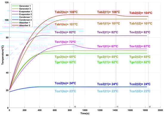
Figure 5.
Behavior of DSHT temperatures over time for Test 1.
During the t0–t1 interval in Test 1, when entering the operating conditions into the ANN, a reduction in the temperature of the first stage evaporator (TEV1) from 72 °C to 67 °C is observed, which optimizes the COP × GTL product. The relationship can be seen in Figure 6, where the pink line represents a TAB2 of 106 °C, and the purple diamond indicates a COP × GTL of 9.3546. The optimal point, identified by the ANN, corresponds to a maximum value of 10.1213 (violet square). This state will be maintained until TAB2 is reduced to 104 °C (a variation of 2 °C) at the user’s discretion, at which point the ANN will adjust the system in the range t1–t2 to reach a new maximum of COP × GTL.
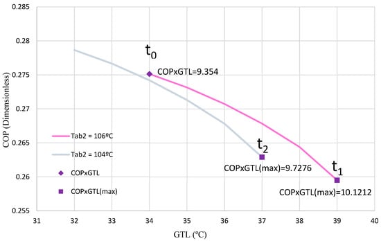
Figure 6.
COP with respect to the GTL for Test 1.
Test 2:
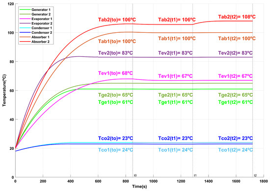
Figure 7.
Behavior of DSHT temperatures over time for Test 2.
In Test 2, the operating conditions introduced into the ANN during the t0–t1 interval cause a decrease in TEV1, maximizing the COP × GTL product. According to Figure 8, the pink line represents TAB2 at 106 °C, while the purple rhombus shows a COP × GTL of 9.9512. The ANN points out that the optimal scenario occurs when the product reaches a maximum value of 9.9899 (violet square). This DSHT status will be maintained until TAB2 is increased to 108 °C, at which point ANN will adapt the system at t1–t2 to achieve the new maximum of the COP × GTL product.
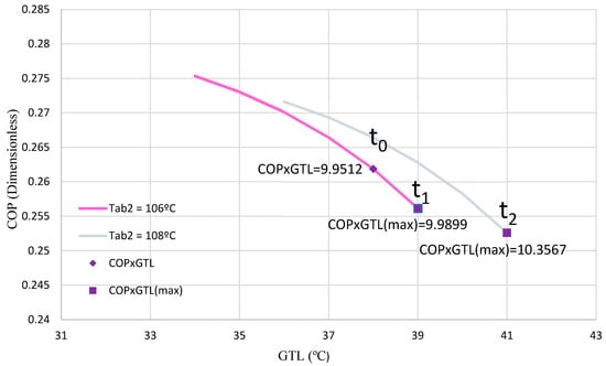
Figure 8.
COP with respect to the GTL for Test 2.
Test 3:
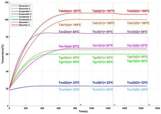
Figure 9.
Behavior of DSHT temperatures over time for Test 3.
During Test 3, between times t0 and t1, the operating conditions processed by the ANN determined that the DSHT remained in an optimal configuration, reaching a maximum COP × GTL of 9.9959. This value, represented by a purple circle and a pink line (with TAB2 set at 107 °C), is illustrated in Figure 10. This condition will be maintained until the user adjusts the TAB2, reducing it by 1 °C. Subsequently, in the t1–t2 interval, the ANN will readjust the system to reach a new maximum value of COP × GTL.
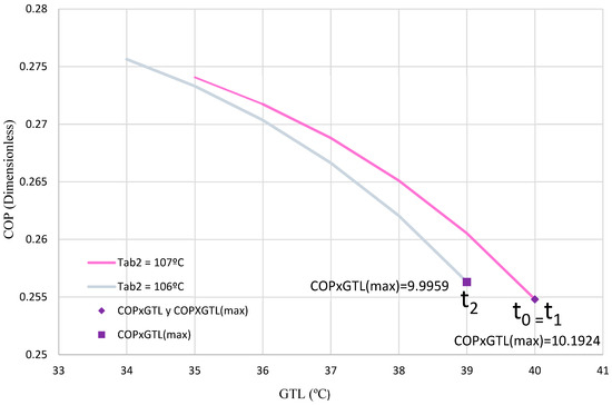
Figure 10.
COP with respect to the GTL for Test 3.
Test 4:
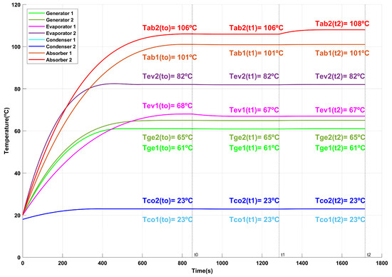
Figure 11.
Behavior of DSHT temperatures over time for Test 4.
During Test 4, in the t0–t1 interval, the conditions entered into the ANN generate a decrease in TEV1 that maximizes COP × GTL. As Figure 12 shows, the pink line reflects TAB2 at 106 °C, and the purple diamond indicates a COP × GTL of 9.9247. The ANN calculates the optimal scenario when this value reaches a maximum of 9.9441 (violet square). The DSHT system will remain in this condition until TAB2 is increased to 108 °C, which will cause the ANN to adjust the system to t1–t2 to reach the new maximum of COP × GTL.
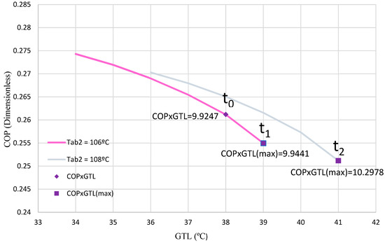
Figure 12.
COP with respect to the GTL for Test 4.
Test 5:
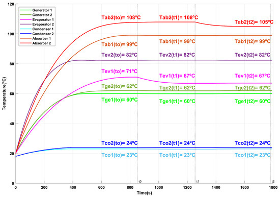
Figure 13.
Behavior of DSHT temperatures over time for Test 5.
In Test 5, the operating conditions processed by the ANN reduce TEV1, thus maximizing the COP × GTL product in the t0–t1 range. In Figure 14, the pink line illustrates a TAB2 of 108 °C, while the purple diamond shows a COP × GTL of 9.5946. According to the ANN, the sweet spot corresponds to a maximum of 10.1096 (violet square). This condition will remain stable until TAB2 is adjusted to 105 °C, after which the ANN will modify the system in the t1–t2 range to ensure the new maximum of the COP × GTL product.
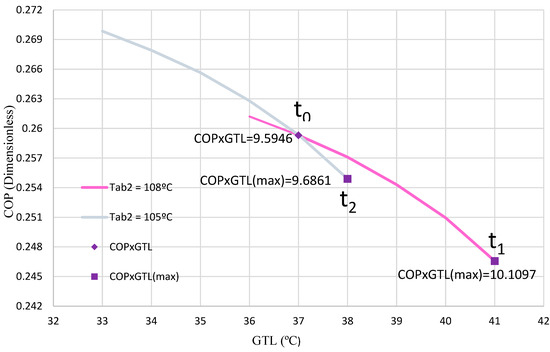
Figure 14.
COP with respect to the GTL for Test 5.
Test 6:
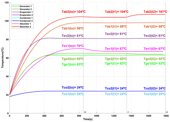
Figure 15.
Behavior of DSHT temperatures over time for Test 6.
In Test 6, between t0–t1, the vector of conditions introduced in the ANN generates an adjustment in TEV1, optimizing the product COP × GTL. Figure 16 illustrates this relationship, showing the pink line for a TAB2 of 104 °C and a purple rhombus indicating a COP × GTL of 9.5716. The ideal scenario is reached with a maximum value of 10.2041 (violet square), according to the ANN. The DSHT system will remain in this optimal state until TAB2 is increased to 107 °C, which will trigger a new adaptation in the t1–t2 range to maintain maximum performance.
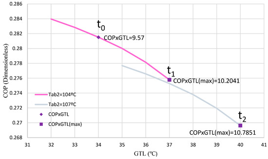
Figure 16.
COP with respect to the GTL for Test 6.
Test 7:
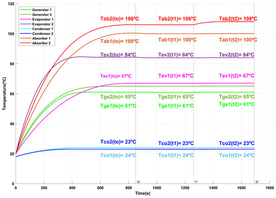
Figure 17.
Behavior of DSHT temperatures over time for Test 7.
In Test 7, during the period t0–t1, the ANN suggests keeping the DSHT in this state, which is where the maximum COP × GTL product is found, with a value of 10.0191. This result, identified by a purple circle and a pink line (TAB2 set to 106 °C), can be seen in Figure 18. The DSHT will continue in this condition until the user modifies the TAB2, increasing it by 2 °C. Accordingly, the ANN will adjust the system again during t1–t2 to ensure the new maximum of COP × GTL.
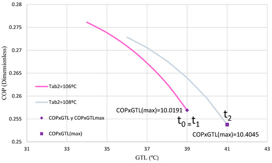
Figure 18.
COP with respect to the GTL for Test 7.
It can be affirmed that using the Levenberg–Marquardt algorithm, we obtained higher values of R for training, validation, and testing. In the case of the scaled conjugate gradient algorithm, it can be seen in Table 10 that in our approximations, for 5, 10, 15, and 20 neurons, the R value for the Levenberg–Marquardt algorithm was always higher and even when we tested with 30 neurons the scaled conjugate gradient algorithm obtained its highest R values 0.99923, 0.999248, and 0.999249 for training, validation, and testing, respectively, without exceeding the Levenberg–Marquardt values of 0.9998414, 0.999826, and 0.999844 for training, validation, and testing, respectively, again.
Table 10.
MSE and R values for the COP × GTL analyzed configurations.
Comparing these values with the previous strategy [3] for calculating a first maximum COP × GTL in the AHT at the first stage and then based on the thermodynamic operating conditions, a second Levenberg–Marquardt for the DSHT was calculated, shown in Table 11, there is a variation with this new machine learning proposal. The previous Levenberg–Marquardt configuration is shown in Figure 19.
Table 11.
MSE and R values for the previous AHT and DSHT configuration.
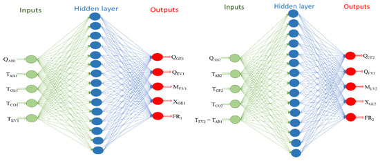
Figure 19.
Previous ANN for Double Stage Heat Transformer [3].
The results demonstrate that the R value for the new algorithm exceeds that of the AHT/DSHT two-step calculation, particularly for the maximum value of the coefficient of performance (COP) at the user-requested absorption temperature. A similar approach was applied for point-to-point network integration across multiple heat sources and users [30].
4. Discussion
In 2025, there are not enough data for controlling double-stage heat transformers based on lithium bromide absorption. There are some data for controlling the temperature in the single-stage heat pump, but the blend was ammonia–water from 80 °C close to 100 °C based on a one-dimensional heat exchanger falling film model [31,32,33], and there is no ANN proposal on that work. Another attempt to control energy recovery has added a compressor with a reduction of the COP and only a single stage [34,35,36,37]. Similar devices based on absorption compression were reported for control with genetic programming without optimal values [38].
In the literature [39], it has been established that the energy for the circulation of liquids in the thermodynamic cycle can be considered small and insignificant, and the flow relationship is always non-linear. Another approach to control a LiBr-H2O AHT is to control the flow [40]. The criterion for determining where a cycle with the highest waste heat recovery temperature can be operated to reintegrate it into the original process, with a circular economy approach, considers that the relationship between the energy that is recovered and the energy that is inputted, already established as COP [41] and that it is modulated between the Gross Temperature Lift (GTL) calculated as the differences in temperatures between the absorber and evaporator.
Reproducing with our ANN the methodology of [14] for the waste energy conditions, but at 70 °C, with an environment at 20 °C, it can be observed in Figure 20, that it only happens in the first stage of the thermodynamic cycle—the best condition to operate is not at the lowest absorption temperature (which obtains the highest COP) and not at the highest absorption temperature (which presents the lowest COP), but is at 114 °C, which is the highest value of the product COP × GTL.
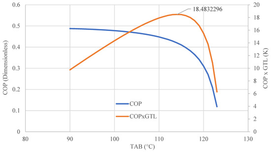
Figure 20.
COP and COP × GTL based on the TAB for a one-stage heat recovery cycle.
In the case of a double stage, using our ANN, we can see the data in Figure 21 and confirm the nonlinear behavior, reported by [14]. Furthermore, it is not possible to identify where a DSHT should operate.
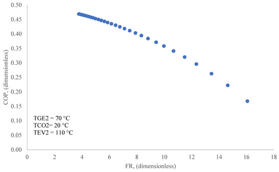
Figure 21.
Performance coefficient as a function of the flow ratio for a DSHT from [14].
In Figure 22, it can be seen that the orange line, corresponding to the methodology presented in this work, allows the identification of the condition in which energy recovery for the circular economy can occur, using the proposed ANN strategy. The maximum TAB2 of the double-stage heat transformer the higher value in the blue line does not indicate the highest COP. Figure 21 shows how the highest value for FR is the lowest value for COP at operating conditions described in Figure 22.
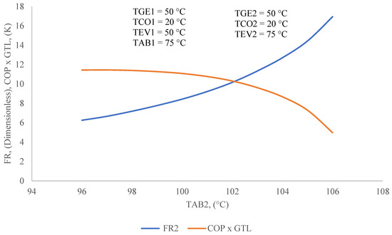
Figure 22.
FR and COP × GTL as a function of the TAB2 of the second stage of a DSHT compared with previous data.
Figure 23 shows that with the data calculated by the ANN, it is possible to determine the optimized operating condition of a DSHT based not on the calculated COP [3]. The optimization on the COP includes the calculation of the energy that can be reintegrated into the process that disposes energy at 70 °C and transfers at 65 °C in the generators and evaporator 1. That energy in the first stage can revalue energy at 85 °C, which is transferred to evaporator 2 at 80 °C. The ANN calculation input determines that in the second stage, energy is added in a second evaporator (QEV2) and therefore the highest temperature of the DSHT is TAB2. Now, with this second stage, the energy will recover at 116 °C—this theoretical calculation shows that the maximum GTL value at the highest possible COP from waste heat is at 70 °C.
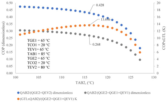
Figure 23.
COP and COP × GTL as a function of the TAB2 of the second stage of a DSHT.
This prediction of the maximum simultaneous values for COP and GTL was achieved and found to be consistent with the thermodynamic values for future energy recycling. This was after evaluating the MSE and R values for the Levenberg–Marquardt (LM) and scaled conjugate gradient (SCG) methods, using five to thirty neurons for training, validation, and testing, as shown in Figure 24. The highest R value, with MSE in the E-05 range, was obtained using the Levenberg–Marquardt method with 15 neurons in the current ANN. In this figure, the lines of the same color were obtained and compared to get the highest R value, as Appendix A shows as a flow diagram. For the scaled conjugate gradient in our previous work, ref. [3] with five neurons, the R value for the training was close to 0.987, with ten being 0.993, fifteen being 0.994, and twenty being 0.992, respectively. Instead, for Levenberg–Marquardt for this work, from five neurons, the R value goes from 0.996 to 0.999 with ten neurons, 0.9996 with fifteen neurons, asymptotic to 1.0. It is remarkable that for 20 neurons, it is the highest R value: 0.999841, while for 25 neurons under training, R value diminishes to 0.999751. Levenberg–Marquardt is always greater than the scaled conjugate gradient from 0.02% to 0.10% with the same data for this study.
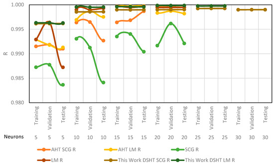
Figure 24.
R values for scaled conjugated gradient and Levenberg–Marquardt algorithms obtained in this work and compared with a previous work [3].
The major improvement occurs when going from five to ten neurons for all cases, which represents a statistical improvement thirty-two times greater compared to increasing from ten to fifteen neurons in training, validation, and testing. From 15 to 20 neurons, the improvement is only two times, but training, validation, and testing from 20 to 25 neurons show a negative improvement, so the selection of neurons remains at 20 neurons.
There are several studies in the literature on the potential of absorption heat pumps in different applications within the industrial sector. In one of these, we work on a proposal integration of a single-state absorption heat pump in a textile industry process (ironing process) [6], without any artificial intelligent algorithm for control; but in this natural step, the implementation is derived from this work. Future work for this research on absorption heat pumps will consist of evaluating whether the algorithm used in this project can be applied to similar processes, where AHTs are already used as an alternative for energy recovery for circular economic processes.
5. Conclusions
An ANN has been designed for a dual-stage absorption heat transformer, configured with 20 neurons in the hidden layer, 360 weights, and 29 biases. The ANN reached a correlation coefficient of 0.9998 and presented MSE values of 1.78592 × 10⁻⁵, 1.97765 × 10⁻⁵, and 1.77207 × 10⁻⁵ for the training, validation, and testing phases, respectively. This model allows calculating the optimal operating conditions to maximize the COP × GTL product.
A computer-aided simulator has been developed to analyze the transient and steady-state behavior of the DSHT temperature variables over time. The tests carried out show that the user-proposed change will cause the developed ANN to create an output vector containing the operating conditions of higher COP × GTL, leading to an MEV1 flow output that will mark the gradual change in the opening or closing of the servo valve.
Using the Levenberg–Marquardt algorithm, higher R values for training, validation, and tests of 0.061%, 0.058%, and 0.060%, respectively, have been obtained. This has resulted in an increase in the simultaneous highest values for COP and GTL. This improvement in energy recovery leads to taking waste energy from 70 °C to a useful circular economy.
Author Contributions
Conceptualization, S.V.-A. and R.J.R.; methodology, S.V.-A., L.D.-G., and R.J.R.; software, S.V.-A., R.J.R. and L.D.-G.; validation, S.V.-A., R.J.R., J.C., and M.M.-G.; formal analysis, S.V.-A., R.J.R., J.C., and M.M.-G.; investigation, S.V.-A. and L.D.-G.; resources, R.J.R.; data curation, S.V.-A. and R.J.R.; writing—original draft preparation, S.V.-A. and R.J.R.; writing—review and editing, S.V.-A., R.J.R., L.D.-G., M.M.-G., and J.C.; visualization, R.J.R. and J.C.; supervision, R.J.R.; project administration, R.J.R.; funding acquisition, R.J.R. All authors have read and agreed to the published version of the manuscript.
Funding
Secretaría de Ciencia Humanidades, Tecnología e Innovación: CVU 9391109.
Data Availability Statement
Research materials necessary to enable the reproduction of an experiment are indicated in Section 2.
Acknowledgments
To UAEM—IICBA—CIICAp Facilities.
Conflicts of Interest
The authors declare no conflicts of interest.
Abbreviations
The following abbreviations are used in this manuscript:
| AHT | Absorption heat transformer |
| ANN | Artificial neural networks |
| COP | Coefficient of performance (dimensionless) |
| DSHT | Double-stage heat transformer |
| FR1 | Flow ratio in AHT (dimensionless) |
| FR2 | Flow ratio in DSHT (dimensionless) |
| GTL | Gross temperature lift (K) |
| MEV1 | Evaporator mass flow in AHT (kg/s) |
| MEV2 | Evaporator mass flow in DSHT (kg/s) |
| MSE | Mean squared error (kg2/s2) |
| QAB2 | Absorption thermal power in DSHT (kW) |
| QGE1 | Desorption thermal power in AHT (kW) |
| QGE2 | Desorption thermal power in DSHT (kW) |
| QEV1 | Evaporation thermal power in AHT (kW) |
| QEV2 | Evaporation thermal power in DSHT (kW) |
| TCO1 | Condenser temperature in AHT (°C) |
| TCO2 | Condenser temperature in DSHT (°C) |
| TEV1 | Evaporator temperature in AHT (°C) |
| TEV2 | Evaporator temperature in DSHT (°C) |
| TAB1 | Absorption temperature in AHT (°C) |
| TAB2 | Absorption temperature in DSHT (°C) |
| R | Strength of correlation (dimensionless) |
Appendix A
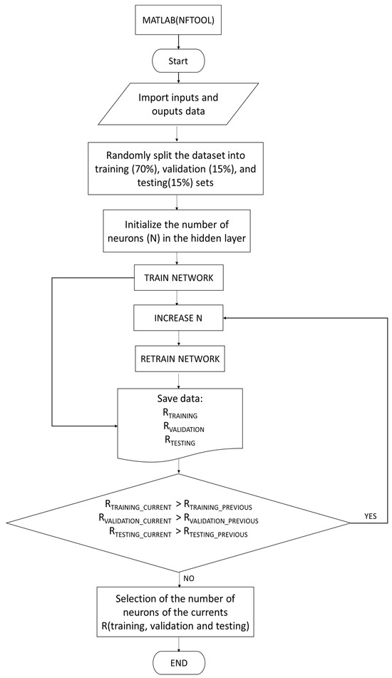
Figure A1.
Flow diagram for obtaining the number of neurons in the hidden layer.
Appendix B
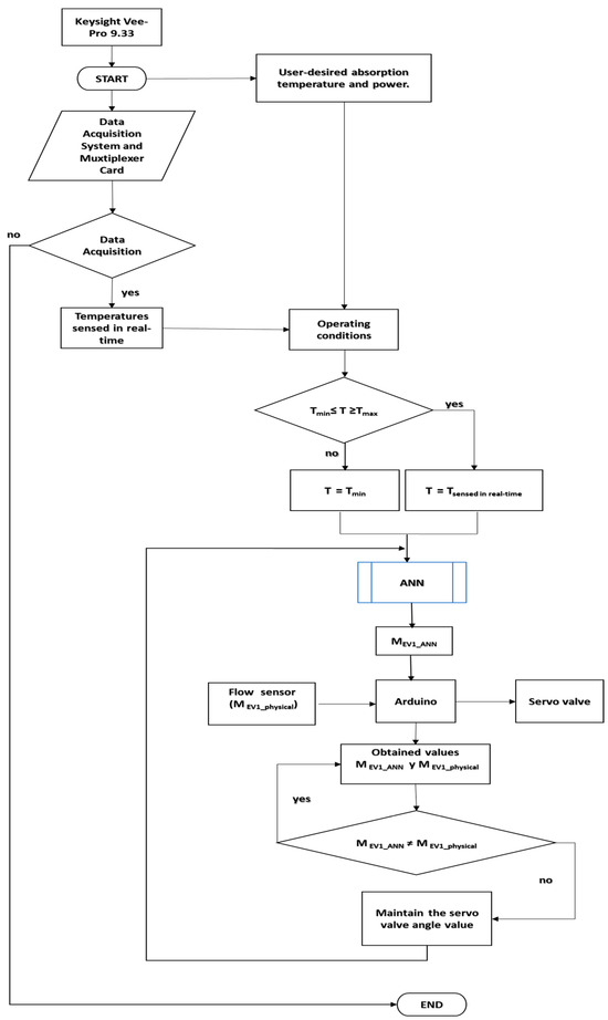
Figure A2.
Flow control diagram MEV1.
Appendix C
References
- Yuan, M.; Mathiesen, B.V.; Schneider, N.; Xia, J.; Zheng, W.; Sorknæs, P.; Lund, H.; Zhang, L. Renewable energy and waste heat recovery in district heating systems in China: A systematic review. Energy 2024, 294, 130788. [Google Scholar] [CrossRef]
- IEA. International Energy Agency. Available online: https://www.iea.org/reports/energy-technology-perspectives-2024 (accessed on 5 November 2024).
- Vázquez-Aveledo, S.; Romero, R.J.; Montiel-González, M.; Cerezo, J. Control Strategy Based on Artificial Intelligence for a Double-Stage Absorption Heat Transformer. Processes 2023, 11, 1632. [Google Scholar] [CrossRef]
- Cudok, F.; Giannetti, N.; Ciganda, J.L.C.; Aoyama, J.; Babu, P.; Coronas, A.; Ziegler, F. Absorption heat transformer-state-of-the-art of industrial applications. Renew. Sustain. Energy Rev. 2021, 141, 110757. [Google Scholar] [CrossRef]
- Romero, R.J.; Cerezo, J.; Rodríguez-Martínez, A.; Montiel, M. Absorption Heat Transformer for Solar Pond Energy Temperature Upgrading. Chem. Eng. Trans. 2021, 86, 703–708. [Google Scholar] [CrossRef]
- Morales-Gómez, L.I.; Romero, R.J.; Vázquez-Aveledo, S.; Montiel-González, M.; Best, R. Energy and environmental study for the textile industry based on absorption heat transformer. Energy Sources Part A Recovery Util. Environ. Eff. 2023, 45, 5594–5607. [Google Scholar] [CrossRef]
- Bora, R.; Richardson, R.; You, F. Resource recovery and waste-to-energy from wastewater sludge via thermochemical conversion technologies in support of circular economy: A comprehensive review. BMC Chem. Eng. 2020, 2, 8. [Google Scholar] [CrossRef]
- Chen, H.; Song, X.; Jian, Y. Performance Assessment of a Municipal Solid Waste Gasification and Power Generation System Integrated with Absorption Heat Pump Drying. Energies 2024, 17, 6034. [Google Scholar] [CrossRef]
- Cai, X.; Wang, Z.; Han, Y.; Su, W. Study on the Performance of a Novel Double-Section Full-Open Absorption Heat Pump for Flue Gas Waste Heat Recovery. Processes 2024, 12, 2181. [Google Scholar] [CrossRef]
- Sun, D.; Liu, Z.; Zhang, H.; Zhang, X. Performance Analysis of a New Cogeneration System with Efficient Utilization of Waste Heat Resources and Energy Conversion Capabilities. Energies 2024, 17, 3347. [Google Scholar] [CrossRef]
- Kabiesz, J.; Kubica, R. Optimizing the Recovery of Latent Heat of Condensation from the Flue Gas Stream through the Combustion of Solid Biomass with a High Moisture Content. Energies 2024, 17, 1670. [Google Scholar] [CrossRef]
- Payá, J.; Cazorla-Marín, A.; Arpagaus, C.; Corrales Ciganda, J.L.; Hassan, A.H. Low-Pressure Steam Generation with Concentrating Solar Energy and Different Heat Upgrade Technologies: Potential in the European Industry. Sustainability 2024, 16, 1733. [Google Scholar] [CrossRef]
- Abbas, T.; Chen, S.; Zhang, X.; Wang, Z. Coordinated Optimization of Hydrogen-Integrated Energy Hubs with Demand Response-Enabled Energy Sharing. Processes 2024, 12, 1338. [Google Scholar] [CrossRef]
- Sotelo, S.S.; Romero, J.R.; Romero, J.R.; Rodríguez-Martínez, A. Double Stage Heat Transformer Controlled by Flow Ratio. In Innovations in Computing Sciences and Software Engineering: Proceedings of the 2009 International Conference on Systems, Computing Sciences and Software Engineering (SCSS), CISSE 09, Bridgeport, CT, USA, 4–12 December 2009; Springer: Dordrecht, The Netherlands, 2009. [Google Scholar] [CrossRef]
- Sajid, M.; Tanveer, M.; Suganthan, P. Ensemble Deep Random Vector Functional Link Neural Network Based on Fuzzy Inference System. IEEE Trans. Fuzzy Syst. 2024, 33, 479–490. [Google Scholar] [CrossRef]
- Dengiz, T.; Kleinebrahm, M. Imitation learning with artificial neural networks for demand response with a heuristic control approach for heat pumps. Energy AI 2024, 18, 100441. [Google Scholar] [CrossRef]
- Rohrer, T.; Frison, L.; Kaupenjohann, L.; Scharf, K.; Hergenrother, E. Deep Reinforcement Learning for Heat Pump Control. In Intelligent Computing. SAI 2023; Arai, K., Ed.; Lecture Notes in Networks and Systems; Springer: Cham, Swizterland, 2023; Volume 711. [Google Scholar] [CrossRef]
- Manjavacas, A.; Campoy-Nieves, A.; Jiménez-Raboso, J.; Molina-Solana, M.; Gómez-Romero, J. An experimental evaluation of deep reinforcement learning algorithms for HVAC control. Artif. Intell. Rev. 2024, 57, 173. [Google Scholar] [CrossRef]
- Sajadi, P.; Rahmani, D.; Mostafa; Tang, Y.; Wang, G. Real-Time Two-Dimensional Temperature Field Prediction in Metal Additive Manufacturing Using Physics-Informed Neural Networks. arXiv 2024, arXiv:2401.02403. [Google Scholar] [CrossRef]
- Yarahmadi, A.M.; Breuß, M.; Hartmann, C. Long Short-Term Memory Neural Network for Temperature Prediction in Laser Powder Bed Additive Manufacturing. In Intelligent Systems and Applications; Arai, K., Ed.; Lecture Notes in Networks and Systems; Springer: Cham, Swizterland, 2023; Volume 544. [Google Scholar] [CrossRef]
- Muravyev, N.V.; Luciano, G.; Ornaghi, H.L., Jr.; Svoboda, R.; Vyazovkin, S. Artificial Neural Networks for Pyrolysis, Thermal Analysis, and Thermokinetic Studies: The Status Quo. Molecules 2021, 26, 3727. [Google Scholar] [CrossRef]
- Zhang, T.; Chen, L.; Wang, J. Multi-objective optimization of elliptical tube fin heat exchangers based on neural networks and genetic algorithm. Energy 2023, 269, 126729. [Google Scholar] [CrossRef]
- Khan, J.; Lee, E.; Kim, K. A higher prediction accuracy–based alpha–beta filter algorithm using the feedforward artificial neural network. CAAI Trans. Intell. Technol. 2023, 8, 1124–1139. [Google Scholar] [CrossRef]
- Villada, F.; Muñoz, N.; García-Quintero, E. Artificial Neural Networks applied to Gold Price Prediction. Inf. Tecnol. 2016, 27, 143–150. [Google Scholar] [CrossRef]
- The MathWorks, Inc. Available online: https://es.mathworks.com/products/deep-learning.html (accessed on 10 May 2024).
- Mishra, S.; Prusty, R.; Hota, P. Analysis of Levenberg-Marquardt and Scaled Conjugate gradient training algorithms for artificial neural network-based LS and MMSE estimated channel equalizers. In Proceedings of the International Conference on Man and Machine Interfacing, Bhubaneswar, India, 17–19 December 2015. [Google Scholar] [CrossRef]
- Valdez, C.V. Design and Modelling of a Two-Stage Thermal Transformer for Waste Heat Recovery with Automatic Control Depending on the Energy to be Revalued. PhD Thesis, Autonomous University of the State of Morelos, Cuernavaca, MR, Mexic, 2019. Available online: http://riaa.uaem.mx/handle/20.500.12055/712 (accessed on 6 January 2025).
- Mantech Electronics. Water Flow Sensor Tutorial. Available online: https://naylampmechatronics.com/sensores-liquido/352-sensor-de-flujo-de-agua-2-yf-dn50.html (accessed on 19 September 2024).
- Heptro. Available online: https://hetpro-store.com/TUTORIALES/pines-arduino/ (accessed on 10 April 2024).
- Wu, W.; Du, Y.; Qian, H.; Fan, H.; Jiang, Z.; Zhang, X.; Huang, S. Enhancing the waste heat utilization of industrial park: A heat pump-centric network integration approach for multiple heat sources and users. Energy Convers. Manag. 2024, 306, 118306. [Google Scholar] [CrossRef]
- Collignon, R.; Demasles, H.; Phan, H.T. Modeling of an Ammonia/Water Absorption Heat Transformer to upgrade low-temperature industrial waste heat both at machine scale and at local scale inside the falling film absorber. Therm. Sci. Eng. Prog. 2025, 59, 103302. [Google Scholar]
- Shen, Z.; Li, S.; Feng, L.; Jin, Z.; Du, K.; Li, Y.; Sheng, W. Performance research of a solution cross-type absorption-resorption heat transformer using NH3/H2O work fluid. Appl. Therm. Eng. 2024, 246, 122874. [Google Scholar]
- Jin, P.; Li, S.; Jin, Z.; Li, Y. Thermodynamic analysis of an ammonia-water double absorption-resorption heat transformer system. Appl. Therm. Eng. 2024, 247, 123130. [Google Scholar]
- Gong, Y.; Liu, F.; Sui, J.; Wang, X.; Jin, H. Thermodynamic performance comparison of H2O/LiBr and ionic liquid working pairs in a novel absorption compression heat transformer system. Therm. Sci. Eng. Prog. 2025, 57, 103115. [Google Scholar]
- Sun, X.; Liu, L.; Zhang, T.; Dai, Y. Multi-objective optimization of a Rectisol process integrated with compression-absorption cascade refrigeration system and ORC for waste heat recovery. Appl. Therm. Eng. 2024, 244, 122611. [Google Scholar] [CrossRef]
- Ji, Q.; Yin, Y.; Huang, G.; Zhao, D.; Cao, B. An advanced cascade method for optimal industrial heating performance in hybrid heat pump. Energy Convers. Manag. 2024, 303, 118187. [Google Scholar] [CrossRef]
- Liu, Y.; Qu, S.; Shen, S.; Feng, Y.; Sun, T.; Wang, C.; Xing, Z. Experimental investigation on the large temperature lift heat pump with an integrated two-stage independently variable frequency compressor. Energy 2025, 314, 134289. [Google Scholar] [CrossRef]
- Wei, J.; Wu, D.; Wang, R. A Multi-Objective evolutionary algorithm-based optimization framework for hybrid absorption-compression heat pump systems. Appl. Energy 2025, 382, 125228. [Google Scholar]
- Romero, R.J.; Cerezo, J.; Martínez, A.R.; Luna, G.H.; Montiel-González, M. On the dimensionless absorption heat pump widespread. J. Adv. Therm. Sci. Res. 2021, 8, 10–20. [Google Scholar] [CrossRef]
- Liu, Z.; Lu, D.; Tao, S.; Chen, R.; Gong, M. Experimental study on using 85° C low-grade heat to generate < 120° C steam by a temperature-distributed absorption heat transformer. Energy 2024, 299, 131491. [Google Scholar] [CrossRef]
- Valdez, V.; Romero, J.R. Optimal design criterion for Heat Transformer operating with Water Carrol. In Proceedings of the Fourth International Conference on Advances in Mechanical and Automation Engineering—MAE 2016, Rome, Italy, 19 August 2016; p. 63. [Google Scholar] [CrossRef]
Disclaimer/Publisher’s Note: The statements, opinions and data contained in all publications are solely those of the individual author(s) and contributor(s) and not of MDPI and/or the editor(s). MDPI and/or the editor(s) disclaim responsibility for any injury to people or property resulting from any ideas, methods, instructions or products referred to in the content. |
© 2025 by the authors. Licensee MDPI, Basel, Switzerland. This article is an open access article distributed under the terms and conditions of the Creative Commons Attribution (CC BY) license (https://creativecommons.org/licenses/by/4.0/).