Assessing the Value of Transfer Learning Metrics for Radio Frequency Domain Adaptation

Abstract

The use of transfer learning (TL) techniques has become common practice in fields such as computer vision (CV) and natural language processing (NLP). Leveraging prior knowledge gained from data with different distributions, TL offers higher performance and reduced training time, but has yet to be fully utilized in applications of machine learning (ML) and deep learning (DL) techniques and applications related to wireless communications, a field loosely termed radio frequency machine learning (RFML). This work examines whether existing transferability metrics, used in other modalities, might be useful in the context of RFML. Results show that the two existing metrics tested, Log Expected Empirical Prediction (LEEP) and Logarithm of Maximum Evidence (LogME), correlate well with post-transfer accuracy and can therefore be used to select source models for radio frequency (RF) domain adaptation and to predict post-transfer accuracy.

1. Introduction

Modern day radio communications systems (Figure 1) allow users to send information across vast distances at near instantaneous speeds. The introduction of ML and DL techniques to modern radio communications systems has the potential to provide increased performance and flexibility when compared to traditional signal processing techniques. For example, cognitive radios (CRs) are capable of autonomously modifying parameters such as the modulation scheme, center frequency, bandwidth, and power in response to the external RF environment to provide continuous, high quality service to the end-user while complying with system and regulatory constraints [1]. While RFML and CR approaches inevitably overlap, RFML differs from CR in that RFML only aims to utilize autonomous feature learning from raw RF data to learn the characteristics to detect, identify, and recognize signals-of-interest [2] and is sometimes used off-board the radio itself and without the intent to re-configure the radio. In other words, RFML approaches can be seen as a component of a larger CR system. Nevertheless, both CR and RFML have broad utility in both the commercial and defense sectors [2,3,4] and are expected to be critical components of the upcoming 6G standard [5].

The RF system overview shown in Figure 1 identifies the parameters/variables that each component of an RF system impacts. Such components make up the domain that may differ significantly across transmitters, receivers, and propagation environments (also known as channels), as well as over time, impacting RFML performance [6]. For example, preliminary results given in [7] showed that the performance of convolutional neural network (CNN) and long short-term memory (LSTM)-based signal classification algorithms trained on data from one transmitter/receiver pair dropped as much as 8% when tested on data captured from other transmitter/receiver pairs even when augmentations were applied to improve performance. Similarly, [8] showed that performance of a CNN-based transmitter identification algorithm degraded significantly when tested on data captured at different times, as well as when tested on data captured in different locations, because the propagation environment had changed. However, the vast majority of existing RFML research focuses on using supervised learning techniques trained from random initialization to perform tasks such as detecting and classifying signals-of-interest [9], without consideration for the changes in domain that will almost certainly be encountered during deployment causing unpredictable and unwanted changes in performance.

Transfer learning (TL) is a means to mitigate such performance degradations by re-using prior knowledge learned from a source domain and task to improve performance on a “similar” target domain and task, as shown in Figure 2. However, the use of TL in RFML algorithms is currently limited and not well understood [6]. Prior work began to address this gap by investigating how the RF domain and task impact learned behavior, facilitating or preventing successful transfer [10]. More specifically, RF TL performance, as measured by post-transfer top-1 accuracy, was evaluated as a function of several metadata parameters-of-interest for a signal classification or automatic modulation classification (AMC) use-case using synthetic datasets. While post-transfer top-1 accuracy provides the ground truth measure of transferability, in the scenario where many source models are available for transfer to an alternate domain, evaluating the post-transfer top-1 accuracy for each source model may be too time consuming and computationally expensive. This work continues to examine RF TL performance across changes in domain specifically using two existing transferability metrics—LEEP [11] and LogME [12]—that provide a measure of how well a source model will transfer to a target dataset using a single forward pass through the source model.

The primary contribution of this work is the application of LEEP and LogME to RFML. Though LEEP and LogME are designed to be modality agnositic, they have not been used in RFML previously. This work shows that both LEEP and LogME strongly correlate with post-transfer top-1 accuracy in the context of this AMC use-case, as well as with each other, and that results are consistent with those shown in the original publications. The application of these metrics to RFML also provides additional insight into RF TL performance and trends, building off of the results given in prior work [10].

Second, we present a method for using transferability metrics such as these to predict post-transfer accuracy within a confidence interval and without further training. More specifically, given a labeled raw In-phase/Quadrature (IQ) target dataset and a selection of pre-trained source models, we show that transferability metrics such as LEEP and/or LogME can be used to provide a lower and upper bound on how well each source model will perform once transferred to the target dataset, without performing head re-training or fine-tuning.

This paper is organized as follows: Section 2 provides requisite background knowledge in RFML, and discusses related and prior works in TL for RFML, transferability metrics, and transfer accuracy prediction in other modalities such as CV and NLP. In Section 3, each of the key methods and systems used and developed for this work are described in detail, including the simulation environment and dataset creation, the model architecture and training, and the transferability metrics. Section 4 presents experimental results and analysis, as well as the proposed post-transfer accuracy prediction method. Section 5 highlights several directions for future work including extensions of this work performed herein using alternative transferability metrics and captured and/or augmented data, generalizations of this work to inductive TL settings, and the development of more robust or RF-specific transferability metrics. Finally, Section 6 offers conclusions about the effectiveness of TL and existing transferability metrics for RFML and the next steps for incorporating and extending TL techniques in RFML-based research. A list of the acronyms used in this work is provided in the appendix for reference.

2. Background and Related Work

2.1. Radio Frequency Machine Learning (RFML)

While the term RFML can be loosely defined as the application of ML or DL to the RF domain, in this work, we use the more rigorous definition of RFML developed by DARPA: the use of DL techniques to reduce the amount of expert-defined features and prior knowledge needed to perform the intended application. This typically means that little-to-no pre-processing is applied to the received signal, which can also reduce latency and computational complexity.

The vast majority of RFML literature has focused on delivering state-of-the-art performance on spectrum awareness and cognitive radio tasks such as signal detection, signal classification or AMC, and spectrum anomaly detection while substantially reducing the expert knowledge needed to perform tradition signal processing techniques. One of the most common, and arguably the most mature spectrum awareness or cognitive radio application explored in the literature, and the example use-case examined in this work is AMC, which is described further in the following sub-section.

2.2. Automatic Modulation Classification (AMC)

AMC is the classification of the format or modulation scheme of a signal-of-interest and is a necessary step in demodulating or recovering the data encoded in a signal [9]. Traditional signal processing approaches to AMC typically consist of a feature extraction stage using hand-crafted “expert features” and a pattern recognition stage [13]. These expert features are pre-defined and designed by a human domain-expert to statistically distinguish between the modulation classes-of-interest and can be time intensive and computationally expensive to extract. Pattern recognition is then performed on these signal features, extracted from the raw RF data during pre-processing, using algorithms such as decision trees, support vector machines (SVMs), or simple neural networks (NNs) to identify the modulation class of the signal-of-interest.

RFML-based approaches both replace the use of hand-crafted expert features using deep NNs, typically CNNs or recurrent neural networks (RNNs), and combine the feature extraction and pattern recognition steps into a single architecture [7,14]. Replacing traditional signal processing techniques with RFML allows for blind and automatic feature learning and classification with little-to-no pre-processing and less prior knowledge and has achieved state-of-the-art performance.

2.3. RF Domain Adaptation

The recent RFML and TL taxonomies and surveys [6,9] highlight the limited existing works that successfully use sequential TL techniques for domain adaptation—transferring pre-trained models across channel environments [15,16], across wireless protocols [17,18], and from synthetic data to real data [19,20,21,22]—for tasks such as signal detection, AMC, and specific emitter identification (SEI). Until recently, little-to-no work has examined what characteristics within RF data facilitate or restrict transfer [6], outside of observing a lack of direct transfer [7,23,24], restricting RF TL algorithms to those borrowed from other modalities, such as CV and NLP. While correlations can be drawn between the vision or language spaces and the RF space, these parallels do not always align, and therefore, algorithms designed for CV and NLP may not always be appropriate for use in RFML.

Our prior work systematically evaluated RF TL performance as a function of signal-tonoise ratio (SNR), frequency offset (FO), and modulation type for an AMC use-case using the same synthetic dataset used herein and a post-transfer top-1 accuracy as the performance metric. (The impact of changing SNR and/or FO on the RF domain is discussed further in Section 3.1.) Across both changes in domain, modeled using changes in SNR and FO, and changes in task, modeled using changes in modulation type, results indicated that source/target similarity was key to successful transfer, as well as domain/task difficulty. More specifically, transfer is more often successful when the source domain/task is more challenging than the target (i.e., the source domain has a lower SNR, or the source task has more output classes than the target task). Discrepancies in the channel environment, as modeled by changes in SNR, were shown to be more challenging to overcome via TL than discrepancies in the RF hardware or platform, as modeled by changes in FO. Additionally, in the cases when TL provided a performance benefit over training from random initialization, head re-training generally outperformed fine-tuning. In this work, post-transfer top-1 accuracy is paired with existing transferability metrics, LEEP and LogME, to further identify how changes in the RF domain impact transferability and for model selection and post-transfer accuracy prediction.

2.4. Transferability Metrics

TL techniques use prior knowledge obtained from a source domain/task to improve performance on a similar target domain/task. More specifically, TL techniques aim to further refine a pre-trained source model using a target dataset and specialized training techniques. However, not all pre-trained source models will transfer well to a given target dataset. Though it is generally understood that TL is successful when the source and target domains/tasks are “similar” [25], this notion of source/target similarity is ill-defined. The goal of a transferability metric is to quantify how well a given pre-trained source model will transfer to a target dataset. While the area of transferability metrics is growing increasingly popular, to our knowledge, no prior works have examined these metrics in the context of RFML. Transferability metrics developed and examined in the context of other modalities can broadly be categorized into one of two types: those requiring partial re-training and those that do not.

Partial re-training methods such as Taskonomy [26] and Task2Vec [27] require some amount of training to occur, whether that be the initial stages of TL, full TL, or the training of an additional probe network, in order to quantify transferability. Partial re-training methods are typically used to identify relationships between source and target tasks and are useful in meta-learning settings but are not well suited to settings where time and/or computational resources are limited. Though the computational complexity of partial re-training methods varies, it vastly exceeds the computational complexity of methods that do not require any additional training, such as those used in this work.

This work focuses on methods that do not require additional training, which typically use a single forward pass through a pre-trained model to ascertain transferability. Methods such as these are often used to select a pre-trained model from a model library for transfer to a target dataset, a problem known as source model selection. LEEP [11] and LogME [12] were chosen as example metrics for this work because they are often used as baselines in the transferability metric literature [28,29,30,31], are designed to be modality agnostic, and have outperformed similar metrics such as Negative Conditional Entropy (NCE) [32] and H-scores [33] in CV and NLP-based experiments. Moreover, LEEP and LogME are intuitive to understand, gauging transferability using the source model’s response to the target dataset in the form of logits or layer activations. More recent transferability metrics that also show promise include Optimal Transport-based Conditional Entropy (OTCE) [29] and Joint Correspondences Negative Conditional Entropy (JC-NCE) [30], TransRate [28], and Gaussian Bhattacharyya Coefficient (GBC) [31] and may be examined as follow-on work. The success of both LEEP and LogME in the context of RFML shown herein suggests that other modality agnostic transferability metrics such as these would also likely be appropriate for use in RFML.

Related works examine source model ranking or selection procedures [34,35], which either rank a set of models by transferability or select the model(s) most likely to provide successful transfer. However, source model ranking or selection methods are less flexible than transferability metrics in online or active learning scenarios. More specifically, source model ranking or selection methods are unable to identify how a new source model compares to the already ranked/selected source models without performing the ranking/selection procedure again. Related works also include methods for selecting the best data to use for pre-training [36] or during the transfer phase [37], and approaches to measuring domain, task, and/or dataset similarity [38].

2.5. Predicting Transfer Accuracy

The problem of predicting transfer accuracy is still an open field. To the best of our knowledge, no prior works have examined predicting transfer accuracy specifically for RFML, but approaches have been developed for other modalities. Most similar to our work is the approach given in [39], where the authors showed a linear correlation between several domain similarity metrics and transfer accuracy, using statistical inference to derive performance predictions for NLP tools. In this work, we show that LEEP and LogME can be used in place of the domain similarity metrics considered in [39] to similar effect. Similarly, work in [40] used domain similarity metrics to predict performance drops as a result in domain shift. However, the domain similarity metrics used in [40] are not easily applicable to RF data, which are high-dimensional, fast-changing, and highly dependent on the underlying bit pattern. More recently, [41] proposed using a simple multi-layer perceptron (MLP) to determine how well a source dataset will transfer to a target dataset, again in an NLP setting. However, the method proposed [41] required the training of an additional model, as well as the use of domain similarity metrics specific to NLP.

3. Methodology

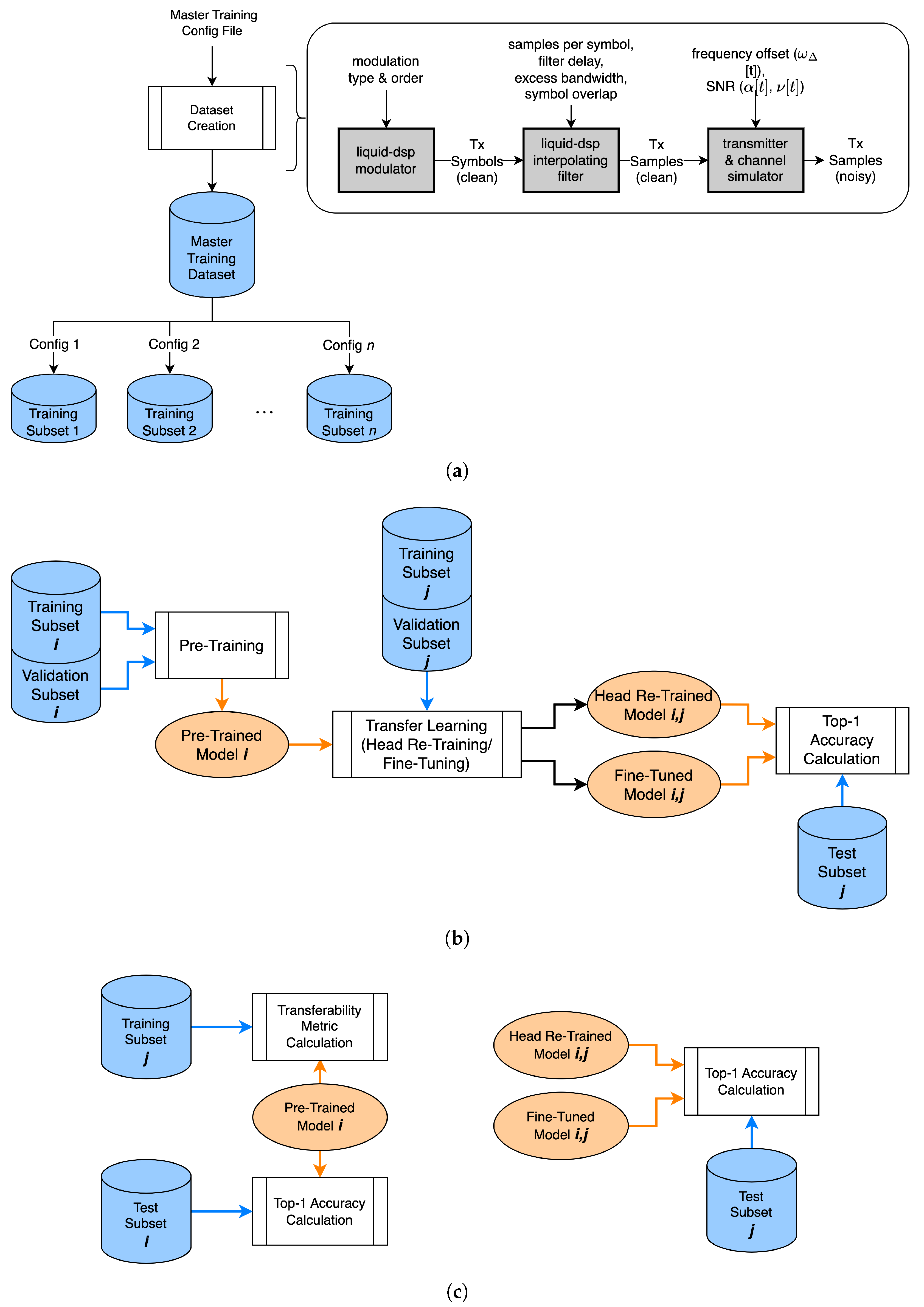
This section presents the experimental setup used in this work, shown in Figure 3, which includes the data and dataset creation process, the model architecture and training, and the transferability metrics. These three key components and processes are each described in detail in the following subsections.

3.1. Dataset Creation

This work uses the same custom synthetic dataset used in our prior work [10], which is publicly available on IEEE DataPort [42]. The dataset creation process, shown in Figure 3a, began with the construction of a large “master” dataset containing 600,000 examples of each of the signal types given in

Table 1. Signal types included in this work and generation parameters.

Modulation Name	Parameter Space
BPSK	Symbol Order {2} RRC Pulse Shape Excess Bandwidth {0.35, 0.5} Symbol Overlap ∈ [3, 5]
QPSK	Symbol Order {4} RRC Pulse Shape Excess Bandwidth {0.35, 0.5} Symbol Overlap ∈ [3, 5]
PSK8	Symbol Order {8} RRC Pulse Shape Excess Bandwidth {0.35, 0.5} Symbol Overlap ∈ [3, 5]
PSK16	Symbol Order {16} RRC Pulse Shape Excess Bandwidth {0.35, 0.5} Symbol Overlap ∈ [3, 5]
OQPSK	Symbol Order {4} RRC Pulse Shape Excess Bandwidth {0.35, 0.5} Symbol Overlap ∈ [3, 5]
QAM16	Symbol Order {16} RRC Pulse Shape Excess Bandwidth {0.35, 0.5} Symbol Overlap ∈ [3, 5]
QAM32	Symbol Order {32} RRC Pulse Shape Excess Bandwidth {0.35, 0.5} Symbol Overlap ∈ [3, 5]
QAM64	Symbol Order {64} RRC Pulse Shape Excess Bandwidth {0.35, 0.5} Symbol Overlap ∈ [3, 5]
APSK16	Symbol Order {16} RRC Pulse Shape Excess Bandwidth {0.35, 0.5} Symbol Overlap ∈ [3, 5]
APSK32	Symbol Order {32} RRC Pulse Shape Excess Bandwidth {0.35, 0.5} Symbol Overlap ∈ [3, 5]
FSK5k	Carrier Spacing {5 kHz} Rect Phase Shape Symbol Overlap {1}
FSK75k	Carrier Spacing {75 kHz} Rect Phase Shape Symbol Overlap {1}
GFSK5k	Carrier Spacing {5 kHz} Gaussian Phase Shape Symbol Overlap {2, 3, 4} Beta ∈ [0.3, 0.5]
GFSK75k	Carrier Spacing {75 kHz} Gaussian Phase Shape Symbol Overlap {2, 3, 4} Beta ∈ [0.3, 0.5]
MSK	Carrier Spacing {2.5 kHz} Rect Phase Shape Symbol Overlap {1}
GMSK	Carrier Spacing {2.5 kHz} Gaussian Phase Shape Symbol Overlap {2, 3, 4} Beta ∈ [0.3, 0.5]
FM-NB	Modulation Index ∈ [0.05, 0.4]
FM-WB	Modulation Index ∈ [0.825, 1.88]
AM-DSB	Modulation Index ∈ [0.5, 0.9]
AM-DSBSC	Modulation Index ∈ [0.5, 0.9]
AM-LSB	Modulation Index ∈ [0.5, 0.9]
AM-USB	Modulation Index ∈ [0.5, 0.9]
AWGN

, for a total of 13.8 million examples. For each example in the master dataset, the SNR is selected uniformly at random within [−10 dB, 20 dB], and the FO is selected uniformly at random within [−10%, 10%] of the sample rate. All further signal generation parameters such as filtering parameters, symbol order, etc., are specified in Table 1.

Then, as in [10], subsets of the master dataset were selected to create different RF domains varying:

• Only SNR—Varying only SNR represents an environment adaptation problem, characterized by a change in the RF channel environment (i.e., an increase/decrease in the additive interference, $\nu \left[t\right]$, of the channel). Twnety-six source data subsets were constructed from the larger master dataset, with SNRs selected uniformly at random from a 5 dB range sweeping from −10 dB to 20 dB in 1 dB steps (i.e., [−10 dB, −5 dB], [−9 dB, −4 dB], …, [15 dB, 20 dB]), and for each data subset in this SNR sweep, FO was selected uniformly at random within [−5%, 5%] of the sample rate.
• Only FO—Varying only FO represents a platform adaptation problem, characterized by a change in the transmitting and/or receiving devices (i.e., an increase/decrease in ${\omega }_{\Delta }\left[t\right]$ due to hardware imperfections or a lack of synchronization). Thirty-one source data subsets were constructed from the larger master dataset containing examples with FOs selected uniformly at random from a 5% range sweeping from −10% of sample rate to 10% of sample rate in 0.5% steps (i.e., [−10%, −5%], [−9.5%, −4.5%], …, [5%, 10%]). For each data subset in this FO sweep, SNR was selected uniformly at random within [0 dB, 20 dB].
• Both SNR and FO—Varying both SNR and FO, represents an environment platform co-adaptation problem, characterized by a change in both the RF channel environment and the transmitting/receiving devices. Twnty-five source data subsets were constructed from the larger master dataset containing examples with SNRs selected uniformly at random from a 10 dB range sweeping from −10 dB to 20 dB in 5 dB steps (i.e., [−10 dB, 0 dB], [−5 dB, 5 dB], …, [10 dB, 20 dB]) and with FOs selected uniformly at random from a 10% range sweeping from −10% of sample rate to 10% of sample rate in 2.5% steps (i.e., [−10%, 0%], [−7.5%, 2.5%], …, [0%, 10%]).

These three parameter sweeps address each type of RF domain adaptation discussed in the RFML TL taxonomy [6].

3.2. Simulation Environment

All data used in this work were generated using the same noise generation, signal parameters, and signal types as in [10]. More specifically, in this work, the signal space has been restricted to the 23 signal types shown in Table 1, observed at a complex baseband in the form of discrete time-series signals, s[t], where

$$s\left[t\right]={\alpha }_{\Delta }\left[t\right]·\alpha \left[t\right]e^{\left(j\omega \right[t]+j\theta [t\left]\right)}·e^{(j{\omega }_{\Delta }\left[t\right]+j{\theta }_{\Delta }\left[t\right])}+\nu \left[t\right]$$

(1)

$\alpha \left[t\right]$, $\omega \left[t\right]$, and $\theta \left[t\right]$ are the magnitude, frequency, and phase of the signal at time t, and $\nu \left[t\right]$ is the additive interference from the channel. Any values subscripted with a $\Delta$ represent imperfections/offsets caused by the transmitter/receiver and/or synchronization. Without loss of generality, all offsets caused by hardware imperfections or lack of synchronization have been consolidated onto the transmitter during simulation.

Signals are initially synthesized in an additive white Gaussian noise (AWGN) channel environment with unit channel gain, no phase offset, and frequency offset held constant for each observation. Like in [10], SNR is defined as

$$\mathrm{SNR}=10{log}_{10}\left({\displaystyle \frac{{\sum }_{t=1}^{N-1}{|s\left[t\right]-\nu \left[t\right]|}^2}{{\sum }_{t=1}^{N-1}{\left|\nu \left[t\right]\right|}^2}}\right)$$

(2)

and with the exception of the AWGN signal that has a Nyquist rate of 1, all signals have a Nyquist rate of either 0.5 or 0.33 (twice or three times the Nyquist bandwidth).

3.3. Model Architecture and Training

The aim of this work is to use the selected metrics to quantify the ability to transfer the features learned by a single architecture trained across pairwise combinations of source/target datasets with varying (1) SNRs, (2) FOs, or (3) SNRs and FO in order to identify the impact of these parameters-of-interest on transferability. Given the large number of models trained for this work, training time was a primary concern when selecting the model architecture. Therefore, this work uses a simple CNN architecture, shown in

Table 2. Model architecture.

Layer Type	Num Kernels/Nodes	Kernel Size
Input	size = (2, 128)
Conv2d	1500	(1, 7)
ReLU
Conv2d	96	(2, 7)
ReLU
Dropout	rate = 0.5
Flatten
Linear	65
Linear	23
Trainable Parameters: 7,434,243

, that is based off of the architectures used in [7].

The model pre-training and TL process is shown in Figure 3b and represents a standard training pipeline. For pre-training, the training dataset contained 5000 examples per class, and the validation dataset contained 500 examples per class. These dataset sizes are consistent with [43] and adequate to achieve consistent convergence. Each model was trained using the Adam optimizer [44] and cross-entropy loss [45], with the PyTorch default hyper-parameters [46] (a learning rate of 0.001, without weight decay), for a total of 100 epochs. A checkpoint was saved after the epoch with the lowest validation loss and was reloaded at the conclusion of the 100 epochs.

As in the prior work [10], both head-retraining and model fine-tuning methods are examined for transfer. For both methods, the training dataset contained 500 examples per class, and the validation dataset contained 50 examples per class, representing a smaller sample of available target data. Both methods also used the Adam optimizer and cross-entropy loss, with checkpoints saved at the lowest validation loss over 100 epochs. However, during head re-training, only the final layer of the model was trained, again using the PyTorch default hyper-parameters, while the rest of the model’s parameters were frozen. During fine-tuning, the entire model was trained with a learning rate of 0.0001, an order of magnitude smaller than the PyTorch default of 0.001 used during pre-training.

3.4. Transferability Metrics

As previously discussed, while transfer accuracy provides the ground truth measure of transferability, calculating transfer accuracy requires performing sequential learning techniques such as head re-training or fine-tuning to completion, in addition to the labeled target dataset. LEEP [11] and LogME [12] are existing metrics designed to predict how well a pre-trained source model will transfer to a labeled target dataset without performing transfer learning techniques and using only a single forward pass through the pre-trained source model. These metrics in particular were shown to outperform similar metrics, NCE [32] and H-scores [33] and are designed to be modality agnostic. Therefore, though neither metric is known to have been shown to correlate with transfer accuracy in the context of RFML, the success both metrics showed in CV and NLP applications bodes well for the RF case.

LEEP [11] can be described as the “average log-likelihood of the expected empirical predictor, a simple classifier that makes prediction[s] based on the expected empirical conditional distribution between source and target labels,” and is calculated as

$$T(f_S,X_T)={\displaystyle \frac{1}{n}}\sum _{i=1}^{n}log\left(\sum _{y_S\in Y_S}\widehat{P}\left(x_T^i\right|y_S)f_S{\left(x_T^i\right)}_{y_S}\right)$$

(3)

such that $f_S$ is the pre-trained source model, $X_T$ is the target dataset, n is the number of examples in the target dataset, $Y_T$ is the set of all target labels, $Y_S$ is the set of all source labels. $\widehat{P}\left(y_T\right|y_S)$ is computed using $\widehat{P}(y_T,y_S)$ and $\widehat{P}\left(y_S\right)$ with

$$\widehat{P}\left(y_T\right|y_S)={\displaystyle \frac{\widehat{P}(y_T,y_S)}{\widehat{P}\left(y_S\right)}}$$

(4)

where

$$\widehat{P}(y_T,y_S)={\displaystyle \frac{1}{n}}\sum _{i:y_T^i=y_T}f{\left(x_T^i\right)}_{y_S}$$

(5)

and

$$\widehat{P}\left(y_S\right)=\sum _{y_T\in Y_T}\widehat{P}(y_T,y_S)={\displaystyle \frac{1}{n}}\sum _{i=1}^{n}f{\left(x_T^i\right)}_{y_S}$$

(6)

Log Expected Empirical Prediction (LEEP) has been shown to correlate well with transfer accuracy using image data, even when the target datasets are small or imbalanced. The metric is bounded between $(-\infty ,0]$, such that values closest to zero indicate best transferability, though the scores tend to be smaller when there are more output classes in the target task. The calculation does not make any assumptions about the similarity of the source/target input data, except that they are the same size. For example, if the source data are raw IQ data of size 2 × 128, then the target data must also be of size 2 × 128 but need not be in raw IQ format (i.e., the target data could be in polar format). Therefore, the metric is suitable for estimating transferability when the source and target tasks (output classes) differ. However, the calculation of the metric does assume the use of a Softmax output layer, limiting the technique to supervised classifiers.

In comparison to LEEP, which measures the expected empirical distribution between the source and target labels, Logarithm of Maximum Evidence (LogME) [12] estimates the maximum evidence, or marginal likelihood, of a label given the features extracted by the pre-trained model at some layer j using a computationally efficient Bayesian algorithm. Letting y be the groundtruth labels of the target dataset, $X_T$, of size n, and D be the dimensionality of the feature space F extracted from the pre-trained model at layer j given $X_T$ as input, LogME is computed as follows: The logarithm of the evidence is computed using

$$\begin{array}{cc}\hfill {\mathrm{argmax}}_{\alpha ,\beta }\mathcal{L}(\alpha ,\beta )& =logp\left(y\right|F,\alpha ,\beta )\hfill \\ \hfill & ={\displaystyle \frac{n}{2}}log\beta +{\displaystyle \frac{D}{2}}log\alpha -{\displaystyle \frac{n}{2}}log2\pi -{\displaystyle \frac{\beta }{2}}{\parallel Fm-y\parallel }_2^2-{\displaystyle \frac{\alpha }{2}}{m}^{T}m-{\displaystyle \frac{1}{2}}log\left|A\right|\hfill \end{array}$$

(7)

where $A=\alpha I+\beta F^{T}T$ and $m=\beta A^{-1}{F}^{T}y$. The full derivation of Equation (7) can be found in [12]. Maximization of $\mathcal{L}(\alpha ,\beta )$ is achieved by iteratively evaluating m and

$$\gamma =\sum _{i=1}^D{\displaystyle \frac{\beta {\sigma }_i}{\alpha +\beta {\sigma }_i}}$$

(8)

with $\sigma$ being the singular values of $F^{T}F$, and updating

$$\alpha \leftarrow {\displaystyle \frac{\gamma }{m^{T}m}},\beta \leftarrow {\displaystyle \frac{n-\gamma }{{\parallel Fm-y\parallel }_2^2}}$$

(9)

until $\alpha$ and $\beta$ converge, generally in 1–3 iterations. Finally, ${\mathrm{argmax}}_{\alpha ,\beta }\mathcal{L}(\alpha ,\beta )$ is scaled by n to compute the average maximum log evidence of $y_i$ given $F_i$ for all $i\in \{1,\dots n\}$, or LogME.

Like LEEP, this calculation only assumes that the source and target input data are the same size. The metric is bounded within [−1, 1], such that values closes to −1 indicate worst transferability, and values closest to 1 indicate best transferability. LogME does not require the use of a Softmax output layer and is therefore appropriate in un-supervised settings, regression settings, and the like. Further, LogME was shown to outperform LEEP in an image classification setting, better correlating with transfer accuracy and has also shown positive results in an NLP setting.

4. Experimental Results and Analysis

The product of the experiments performed herein is 82 data subsets, each with distinct RF domains, 82 source models trained from random initialization, and 4360 transfer learned models, half transferred using head re-training and the remaining half transferred using fine-tuning. Associated with each of the 4360 transfer learned models is a top-1 accuracy value, a LEEP score, and a LogME score. The following subsections present the results obtained from the experiments performed and discuss how well LEEP and LogME perform in the RF modality, how to use transferability metrics to predict post-transfer performance, as well as some insights and practical takeaways that can be gleaned from the results given, including a preliminary understanding of when and how to use TL for RF domain adaptation.

4.1. Transferability Metrics for Model Selection in RF Domain Adaptation

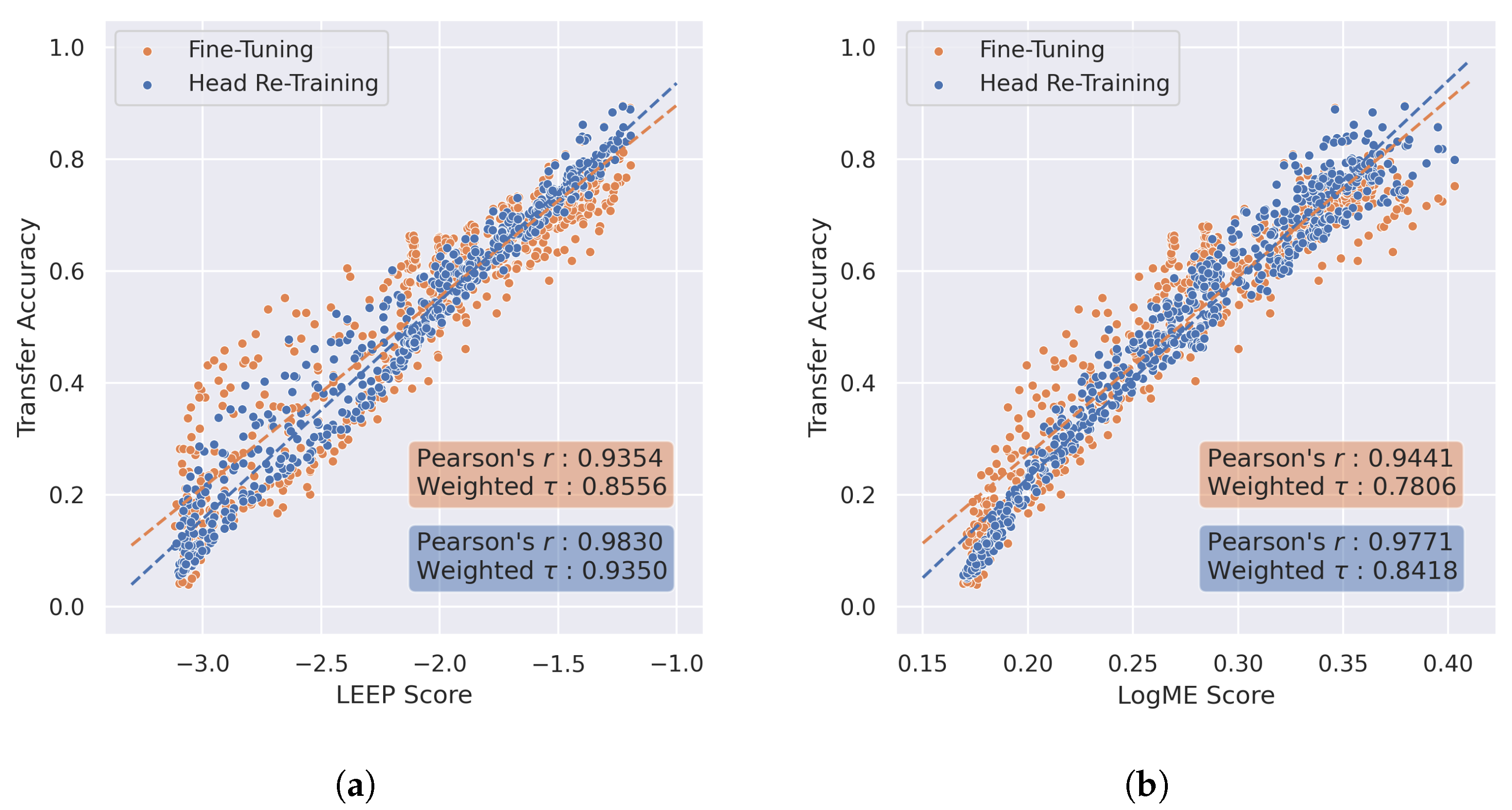
When evaluating whether a transferability metric is accurate, the primary consideration is how well the metric reflects or correlates with the performance metric(s) used. Therefore, to identify whether LEEP and/or LogME can be used to select models for RF domain adaptation is to identify how well LEEP and LogME correlate with post-transfer top-1 accuracy. To this end, Figure 4, Figure 5 and Figure 6 show LEEP and LogME versus the achieved transfer accuracy for each of the parameter sweeps described in Section 3.1. These figures qualitatively show that both LEEP and LogME correlate well with top-1 accuracy after transfer learning, whether through head re-training or fine-tuning for all domain adaptation settings studied.

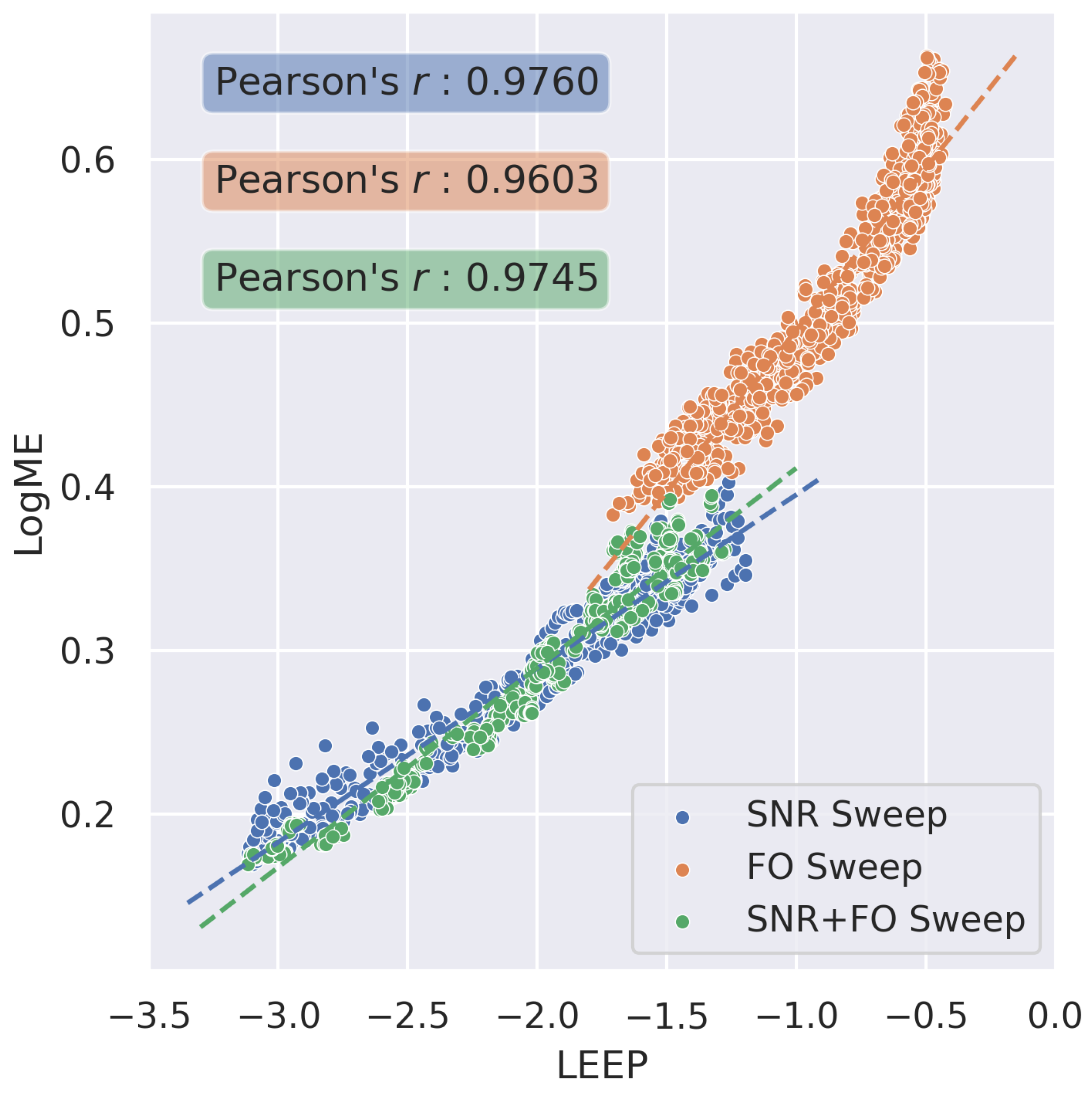
To quantify whether or not the metrics are useful, two correlation measures are also examined—the Pearson correlation coefficient [47] and the weighted $\tau$ [48]—and specified in the shaded boxes of Figure 4, Figure 5 and Figure 6. The Pearson correlation coefficient, or Pearson’s r, is a measure of linear correlation between two variables used in a wide variety of works, including the original LEEP paper. However, Pearson’s r makes a number of assumptions about the data, some of which may not be met by these data. Most notably, Pearson’s r assumes that both variables (LEEP/LogME and post-transfer top-1 accuracy, herein) are normally distributed and have a linear relationship. Alternatively, weighted $\tau$, a weighted version of the Kendall rank correlation coefficient (Kendall $\tau$), is used in the original LogME work. Weighted $\tau$ is a measure of correspondence between pairwise rankings, where higher performing/scoring models receive higher weight, and it only assumes the variables (LEEP/LogME and post-transfer top-1 accuracy, herein) are continuous. Both Pearson’s r and weighted $\tau$ have a range of [−1,1]. These correlation coefficients confirm the results discussed above. Finally, Figure 7 confirms the LEEP and LogME scores are highly linearly correlated with each other.

From these figures and metrics, it can be concluded that both LEEP and LogME are strong measures for selecting models for RF domain adaptation. However, head re-training is more consistent with LEEP and LogME scores than fine-tuning, as evidenced by higher correlation coefficients. Therefore, when using LEEP or LogME for model selection, using head re-training as a TL method would be more reliable than using fine-tuning. In contrast, fine-tuning, while less reliable than head re-training when used in conjunction with LEEP or LogME for model selection, offers potential for small performance gains over head re-training. In practice, this indicates that unless top performance is of more value than reliability, head re-training should be used for TL when using LEEP or LogME for model selection. In the setting where model accuracy is of the utmost importance, it may be advantageous to try both head re-training and fine-tuning.

It should also be noted that the results shown in Figure 4, Figure 5 and Figure 6 are consistent with the results presented in the original LEEP and LogME publications where the metrics were tested in CV and NLP settings, supporting the claim that these metrics are truly modality agnostic. Therefore, other modality agnostic metrics seem likely to perform well in RFML settings as well and may be examined as follow-on work.

4.2. When and How RF Domain Adaptation Is Most Successful

4.2.1. Environment Adaptation vs. Platform Adaptation

Recalling that the sweep over SNR can be regarded as an environment adaptation experiment and the sweep over FO can be regarded as a platform adaptation experiment, more general conclusions can be drawn regarding the challenges that environment and platform adaptation present. Results given in prior work [6] indicated that changes in FO are easier to overcome than changes in SNR. That is, environment adaptation is more difficult to achieve than platform adaptation, and changes in transmitter/receiver hardware are likely easier to overcome using TL techniques than changes in the channel environment. This trend is also shown in Figure 7, which presents the LogME scores as a function of the LEEP scores for each of the parameter sweeps performed, showing both the LEEP and LogME scores are significantly higher for the FO sweep than the SNR sweep or SNR and FO sweep, indicating better transferability. Of course, this conclusion is dependent upon the results presented in Section 4.1, which show that LEEP and LogME correlate with post-transfer accuracy. Therefore, in practice, one should consider the similarity of the source/target channel environment before the similarity of the source/target platform, as changes in the transmitter/receiver pair are more easily overcome during TL.

4.2.2. Head Re-Training vs. Fine-Tuning

In our prior work, results showed that in the cases when TL provided a performance benefit over training from random initialization, head re-training generally outperformed fine-tuning. This trend is also evident in Figure 4, Figure 5 and Figure 6. However, in the sweep over FO, especially when the LEEP and LogME scores were low, the fine-tuned models markedly outperformed head re-trained models. A low LEEP/LogME score indicates a significant change between the source and target domains, and in this case, a large change in FO. As a result, new features are needed to discern between modulation types, and modifications to the earlier layers of the pre-trained source model, where feature learning occurs, are needed in order to best adapt to the new target domain. However, head re-training is more time efficient and less computationally expensive than fine-tuning, making a strong case for using head re-training over fine-tuning for RF domain adaptation. The computational complexity of using head re-training versus fine-tuning is architecture- and training algorithm-dependent, but as an example, for the CNN architecture used in this work and shown in Table 2, the number of trainable parameters for head re-training and fine-tuning is 1518 and 7,434,243, respectively.

4.3. Transferability Metrics for Predicting Post-Transfer Accuracy

Having confirmed that LEEP and LogME strongly correlate with post-transfer top-1 accuracy, it can be concluded that these metrics can be used to compare the transferability of n source models to a single target dataset (i.e., whichever model provides the highest LEEP/LogME score is most likely to provide the best transfer). What follows is an approach to not only select or compare models for RF domain adaptation but also to predict the post-transfer top-1 accuracy without any further training. The approach is time- and resource-intensive to initialize, but once initialized, is fast and relatively inexpensive to compute and shows the predictive capabilities of these metrics. It should be noted that the cost of initialization can be mitigated somewhat by using only a subset of the available source/target pairs. However, the more source/target pairs used, the better the quality of the transfer accuracy prediction and confidence interval.

Given n known domains and assuming a single model architecture, to initialize the approach:

• Run baseline simulations for all n known domains, including pre-training source models on all domains, and use head re-training and/or fine-tuning to transfer each source model to the remaining known domains
• Compute LEEP/LogME scores using all n pre-trained source models and the remaining known domains.
• Compute post-transfer top-1 accuracy for all n transfer-learned models, constructing datapoints like those displayed in Figure 4, Figure 5 and Figure 6.
• Fit a function of the desired form (i.e., linear, logarithmic, etc.) to the LEEP/LogME scores and post-transfer top-1 accuracies. For example, a linear fit of the form $y={\beta }_{0}x+{\beta }_1$ is shown in Figure 4, Figure 5 and Figure 6 such that x is the transferability score and y is the post-transfer top-1 accuracy.
• Compute the margin of error by first calculating the mean difference between the true post-transfer top-1 accuracy and the predicted post-transfer top-1 accuracy (using the linear fit), and then multiply this mean by the appropriate z-score(s) for the desired confidence interval(s) [49].

Then, during deployment, given a newly labeled target dataset:

• Compute LEEP/LogME scores for all pre-trained source models and the new target dataset.
• Select the pre-trained source model yielding the highest LEEP/LogME score for TL.
• Use the fitted linear function to estimate post-transfer accuracy, given the highest LEEP/LogME score, and add/subtract the margin of error to construct the confidence interval.

Optionally, after transferring to the new labeled target dataset, add this dataset to the list of known domains and update the linear fit and margin of error, as needed.

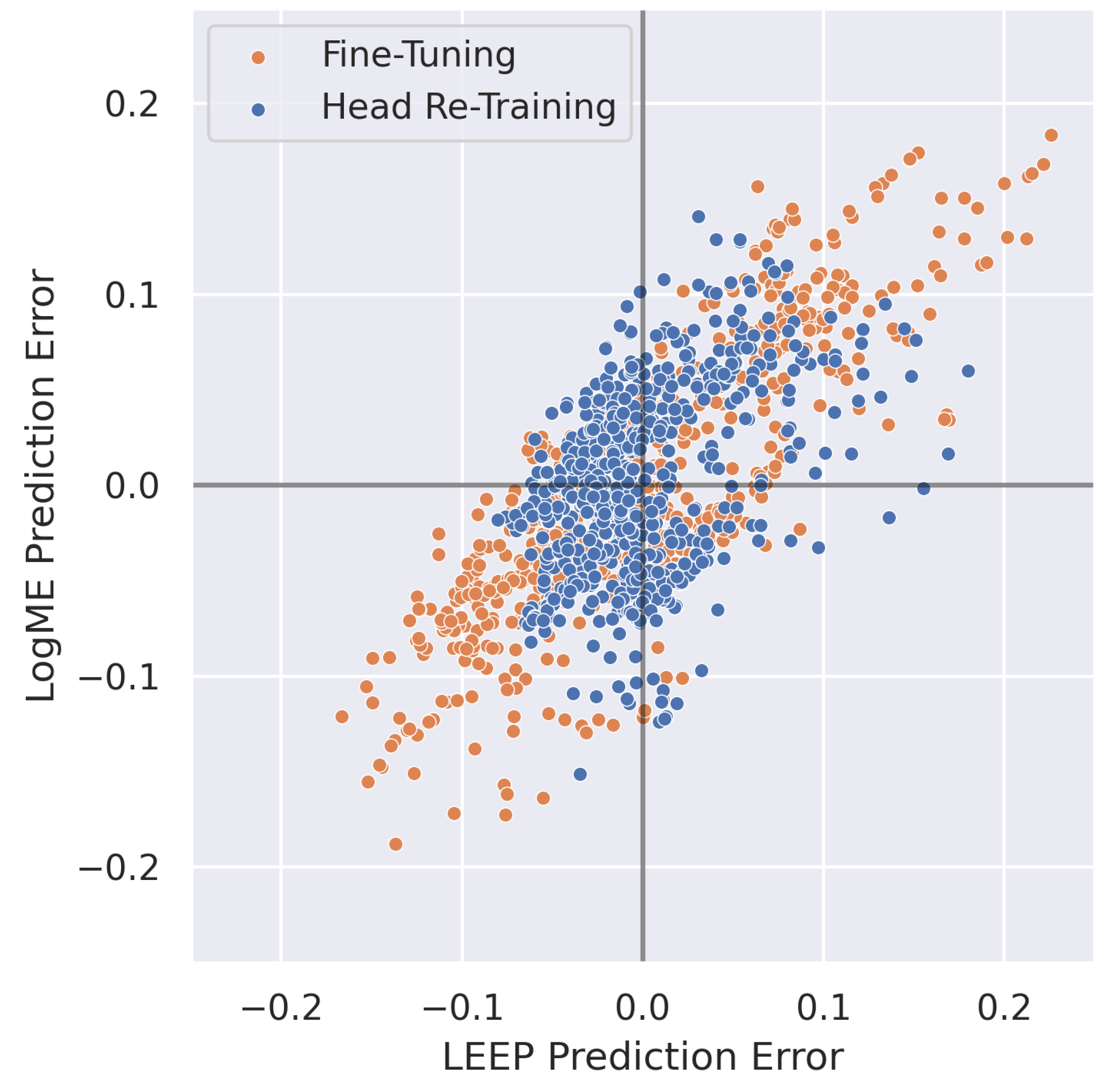
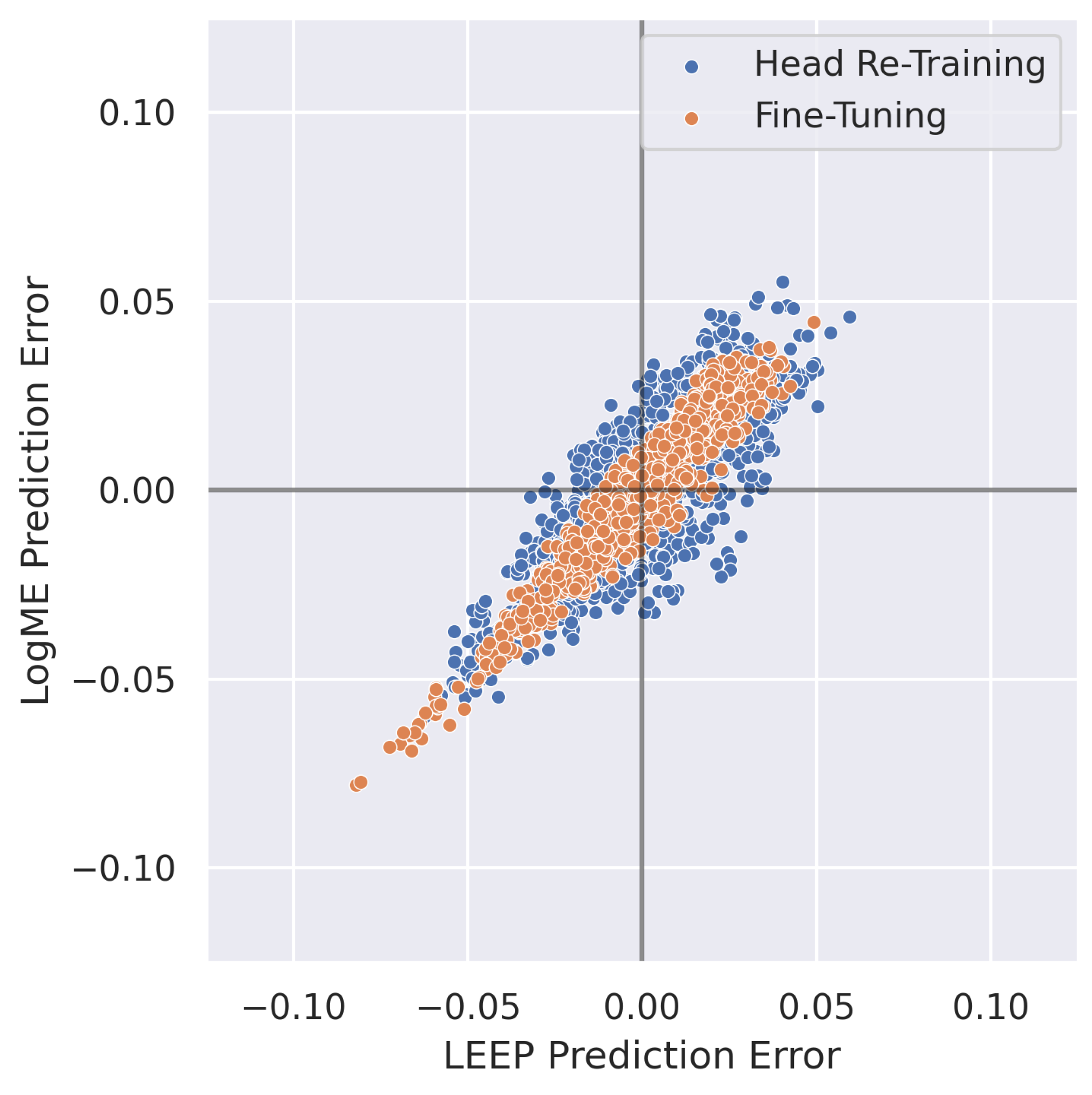
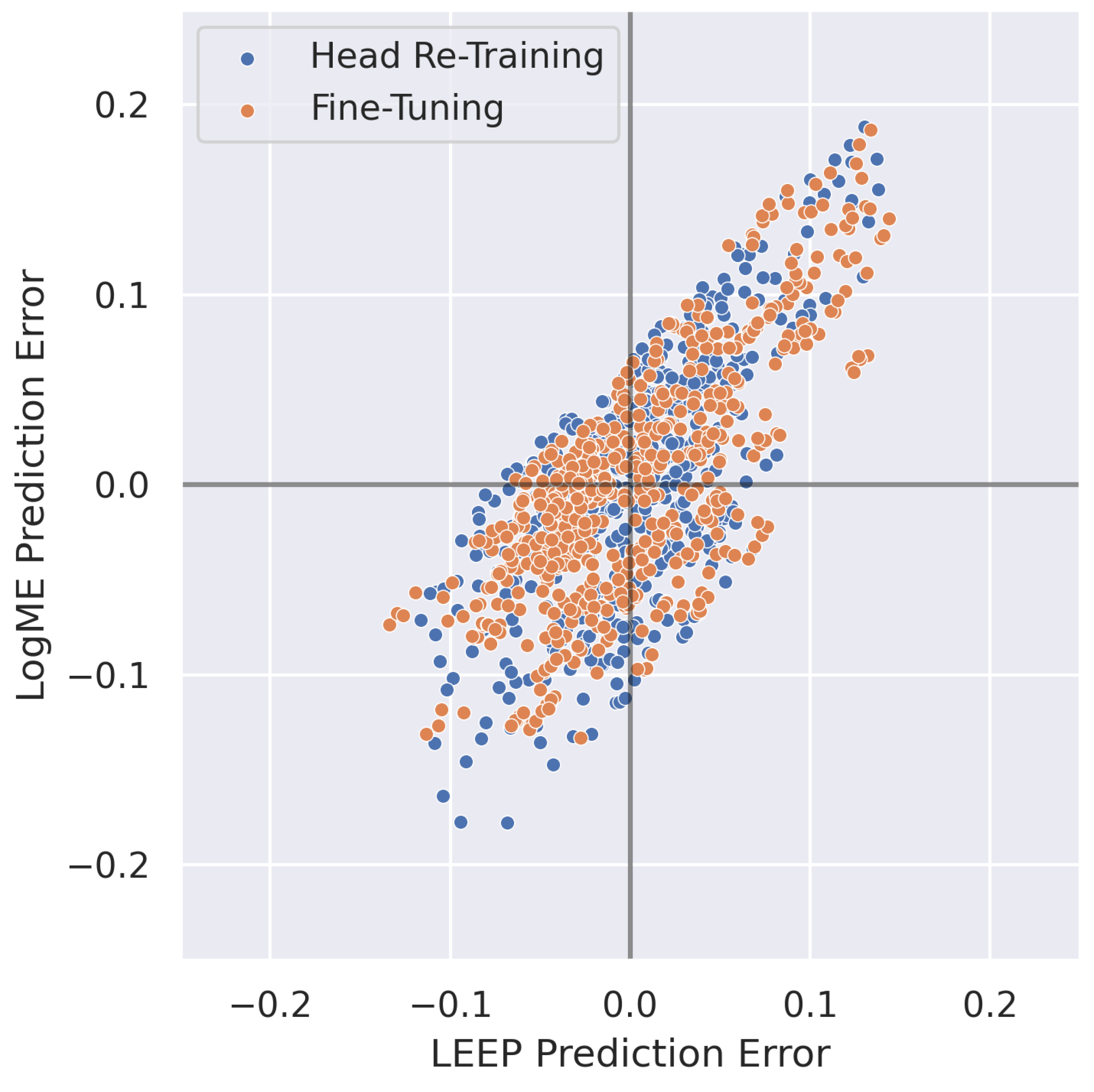
The error in the predicted post-transfer accuracy using the proposed method is shown in Figure 8, Figure 9 and Figure 10. These plots show that not only are LEEP/LogME highly correlated with post-transfer top-1 accuracy (as shown in Figure 4, Figure 5 and Figure 6), but the error in the predicted post-transfer top-1 accuracy using a linear fit to the LEEP and LogME scores, respectively, is also highly correlated. More specifically, when the proposed method constructed using LEEP predicts a lower/higher post-transfer accuracy than ground truth, the proposed method constructed using LogME will do the same with the frequencies shown in

Table 3. The frequency with which the proposed method constructed using LEEP and LogME agree in over/under-predicting post-transfer accuracy.

	SNR Sweep	FO Sweep	SNR + FO Sweep
Head Re-Training	0.6175	0.7856	0.7258
Fine-Tuning	0.7496	0.8803	0.7468

. This indicates that these scores could be combined to create a more robust transferability metric and more robust post-transfer accuracy prediction with relative ease, which is left for future work.

5. Future Work

As previously mentioned, several new transferability metrics were developed concurrently with this work and are suitable as replacements for LEEP and LogME in any of the above experiments. Therefore, the first direction for future work is replicating this work using alternative metrics, such as OTCE [29], JC-NCE [30], TransRate [28], and GBC [31], to identify if these metrics are also suitable for use in the context of RFML and if these metrics might outperform those used herein. Given that this work supports the claim that LEEP and LogME are modality agnostic, it seems likely that additional transferability metrics that are also modality agnostic by design will also follow this trend. Additionally, the concept of transferability metrics and the experiments performed herein should be extended to inductive TL settings, including multi-task learning and sequential learning settings in which the source and target tasks differ (i.e., adding/removing output classes), as well as to different model architectures, as this work only considered RF domain adaptation.

Another direction for future work is the development of new transferability metrics that are more robust than LEEP or LogME alone or are RFML-specific. Most apparently, results discussed previously in Section 4.3 indicate that LEEP and LogME could be combined to create a more robust transferability metric with relative ease. However, while modality agnostic metrics such as LEEP and LogME are shown herein to be suitable for use in RFML, a transferability metric purpose-built for the RF space would likely be more widely accepted amongst traditional RF engineers [9].

Towards such an approach, transferability can be gauged in numerous, potentially synergistic, ways. While metrics such as LEEP and LogME measure the source model’s activations in response to the target dataset, a supplementary approach could include quantifing the similarity between the source and target datasets, independent of the source model.

Finally, this work provided additional conclusions about how best to use TL in the context of RFML, which should be verified and refined with experiments using captured and augmented data [23]. If verified, these metrics could be used to select RFML models or predict transfer performance for online or incremental learning during continuous deployment to help overcome the highly fluid nature of modern communication systems [9].

6. Conclusions

TL has yielded tremendous performance benefits in CV and NLP, and as a result, TL is all but commonplace in these fields. However, the benefits of TL have yet to be fully demonstrated and integrated into RFML systems. While prior work began addressing this deficit by systematically evaluating RF domain adaptation performance as a function of several parameters-of-interest, this work introduced two existing transferability metrics, LEEP and LogME. Results presented herein demonstrated that LEEP and LogME correlate well with post-transfer accuracy and can therefore be used for model selection in the context of RF domain adaptation. The addition of these metrics also provided further insight into RF TL performance trends, generally echoing the guidelines for when and how to use RF TL presented in [10]. Finally, an approach was presented for predicting post-transfer accuracy using these metrics within a confidence interval and without further training.

References

1. Mitola, J. Cognitive Radio: An Integrated Agent Architecture for Software Defined Radio. Ph.D. Dissertation, Royal Institute of Technology, Stockholm, Sweden, 2000. [Google Scholar]
2. Rondeau, T. Radio Frequency Machine Learning Systems (RFMLS). 2017. Available online: https://www.darpa.mil/program/radio-frequency-machine-learning-systems (accessed on 24 March 2022).
3. Kolb, P. Securing Compartmented Information with Smart Radio Systems (SCISRS). 2021. Available online: https://www.iarpa.gov/index.php/research-programs/scisrs (accessed on 24 March 2022).
4. Conference, IEEE Communications Society. In Proceedings of the DySPAN 2021: 2020 IEEE International Symposium on Dynamic Spectrum Access Networks, Los Angeles, CA, USA, 13–15 December 2021. Available online: https://dyspan2021.ieee-dyspan.org/index.html (accessed on 24 March 2024).
5. Morocho-Cayamcela, M.E.; Lee, H.; Lim, W. Machine Learning for 5G/B5G Mobile and Wireless Communications: Potential, Limitations, and Future Directions. IEEE Access 2019, 7, 137184–137206. [Google Scholar] [CrossRef]
6. Wong, L.J.; Michaels, A.J. Transfer Learning for Radio Frequency Machine Learning: A Taxonomy and Survey. Sensors 2022, 22, 1416. [Google Scholar] [CrossRef]
7. Hauser, S.C. Real-World Considerations for Deep Learning in Spectrum Sensing. Master’s Thesis, Virginia Tech, Blacksburg, VA, USA, 2018. [Google Scholar]
8. Sankhe, K.; Belgiovine, M.; Zhou, F.; Riyaz, S.; Ioannidis, S.; Chowdhury, K. ORACLE: Optimized Radio Classification through Convolutional Neural Networks. In Proceedings of the IEEE INFOCOM 2019-IEEE Conference on Computer Communications, Paris, France, 29 April 2019–2 May 2019; IEEE: Piscataway Township, NJ, USA, 2019; pp. 370–378. [Google Scholar]
9. Wong, L.J.; Clark, W.H.; Flowers, B.; Buehrer, R.M.; Headley, W.C.; Michaels, A.J. An RFML Ecosystem: Considerations for the Application of Deep Learning to Spectrum Situational Awareness. IEEE Open J. Commun. Soc. 2021, 2, 2243–2264. [Google Scholar] [CrossRef]
10. Wong, L.J.; Muller, B.P.; McPherson, S.; Michaels, A.J. An Analysis of Radio Frequency Transfer Learning Behavior. Mach. Learn. Knowl. Extr. 2024, 6, 57. [Google Scholar] [CrossRef]
11. Nguyen, C.; Hassner, T.; Seeger, M.; Archambeau, C. LEEP: A new measure to evaluate transferability of learned representations. In Proceedings of the International Conference on Machine Learning, PMLR, Online, 13–18 July 2020; pp. 7294–7305. [Google Scholar]
12. You, K.; Liu, Y.; Long, M.; Wang, J. LogME: Practical Assessment of Pre-trained Models for Transfer Learning. arXiv 2021, arXiv:2102.11005. [Google Scholar]
13. Dobre, O.A.; Abdi, A.; Bar-Ness, Y.; Su, W. Survey of automatic modulation classification techniques: Classical approaches and new trends. IET Commun. 2007, 1, 137–156. [Google Scholar] [CrossRef]
14. West, N.E.; O’Shea, T. Deep architectures for modulation recognition. In Proceedings of the 2017 IEEE International Symposium on Dynamic Spectrum Access Networks (DySPAN), Baltimore, MD, USA, 6–9 March 2017; pp. 1–6. [Google Scholar]
15. Chen, S.; Zheng, S.; Yang, L.; Yang, X. Deep Learning for Large-Scale Real-World ACARS and ADS-B Radio Signal Classification. IEEE Access 2019, 7, 89256–89264. [Google Scholar] [CrossRef]
16. Pati, B.M.; Kaneko, M.; Taparugssanagorn, A. A Deep Convolutional Neural Network Based Transfer Learning Method for Non-Cooperative Spectrum Sensing. IEEE Access 2020, 8, 164529–164545. [Google Scholar] [CrossRef]
17. Kuzdeba, S.; Robinson, J.; Carmack, J. Transfer Learning with Radio Frequency Signals. In Proceedings of the 2021 IEEE 18th Annual Consumer Communications Networking Conference (CCNC), Las Vegas, NV, USA, 9–12 January 2021; pp. 1–9. [Google Scholar] [CrossRef]
18. Robinson, J.; Kuzdeba, S. RiftNet: Radio Frequency Classification for Large Populations. In Proceedings of the 2021 IEEE 18th Annual Consumer Communications Networking Conference (CCNC), Las Vegas, NV, USA, 9–12 January 2021; pp. 1–6. [Google Scholar] [CrossRef]
19. O’Shea, T.J.; Roy, T.; Clancy, T.C. Over-the-Air Deep Learning Based Radio Signal Classification. IEEE J. Sel. Top. Signal Process. 2018, 12, 168–179. [Google Scholar] [CrossRef]
20. Dörner, S.; Cammerer, S.; Hoydis, J.; Brink, S.t. Deep Learning Based Communication Over the Air. IEEE J. Sel. Top. Signal Process. 2018, 12, 132–143. [Google Scholar] [CrossRef]
21. Zheng, S.; Chen, S.; Qi, P.; Zhou, H.; Yang, X. Spectrum sensing based on deep learning classification for cognitive radios. China Comm. 2020, 17, 138–148. [Google Scholar] [CrossRef]
22. Clark, B.; Leffke, Z.; Headley, C.; Michaels, A. Cyborg Phase II Final Report; Technical report; Ted and Karyn Hume Center for National Security and Technology: Blacksburg, VA, USA, 2019. [Google Scholar]
23. Clark IV, W.H.; Hauser, S.; Headley, W.C.; Michaels, A.J. Training data augmentation for deep learning radio frequency systems. J. Def. Model. Simul. 2020, 18, 154851292199124. [Google Scholar] [CrossRef]
24. Merchant, K. Deep Neural Networks for Radio Frequency Fingerprinting. PhD Thesis, University of Maryland, College Park, MD, USA, 2019. [Google Scholar]
25. Pan, S.J.; Yang, Q. A Survey on Transfer Learning. IEEE Trans. Knowl. Data Eng. 2010, 22, 1345–1359. [Google Scholar] [CrossRef]
26. Zamir, A.R.; Sax, A.; Shen, W.; Guibas, L.J.; Malik, J.; Savarese, S. Taskonomy: Disentangling task transfer learning. In Proceedings of the IEEE Conference on Computer Vision and Pattern Recognition, Salt Lake City, UT, USA, 18–23 June 2018; pp. 3712–3722. [Google Scholar]
27. Achille, A.; Lam, M.; Tewari, R.; Ravichandran, A.; Maji, S.; Fowlkes, C.C.; Soatto, S.; Perona, P. Task2Vec: Task embedding for meta-learning. In Proceedings of the IEEE/CVF International Conference on Computer Vision, Seoul, Republic of Korea, 27 October 2019–2 November 2019; pp. 6430–6439. [Google Scholar]
28. Huang, L.K.; Wei, Y.; Rong, Y.; Yang, Q.; Huang, J. Frustratingly Easy Transferability Estimation. arXiv 2021, arXiv:2106.09362. [Google Scholar]
29. Tan, Y.; Li, Y.; Huang, S.L. OTCE: A Transferability Metric for Cross-Domain Cross-Task Representations. In Proceedings of the IEEE/CVF Conference on Computer Vision and Pattern Recognition, Nashville, TN, USA, 20–25 June 2021; pp. 15779–15788. [Google Scholar]
30. Tan, Y.; Li, Y.; Huang, S.L. Practical Transferability Estimation for Image Classification Tasks. arXiv 2021, arXiv:2106.10479. [Google Scholar]
31. Pándy, M.; Agostinelli, A.; Uijlings, J.; Ferrari, V.; Mensink, T. Transferability Estimation using Bhattacharyya Class Separability. arXiv 2021, arXiv:2111.12780. [Google Scholar]
32. Tran, A.T.; Nguyen, C.V.; Hassner, T. Transferability and hardness of supervised classification tasks. In Proceedings of the IEEE/CVF International Conference on Computer Vision, Seoul, Republic of Korea, 27 October 2019–2 November 2019; pp. 1395–1405. [Google Scholar]
33. Bao, Y.; Li, Y.; Huang, S.L.; Zhang, L.; Zheng, L.; Zamir, A.; Guibas, L. An Information-Theoretic Approach to Transferability in Task Transfer Learning. In Proceedings of the 2019 IEEE International Conference on Image Processing (ICIP), Taipei, Taiwan, 22–25 September 2019; pp. 2309–2313. [Google Scholar] [CrossRef]
34. Renggli, C.; Pinto, A.S.; Rimanic, L.; Puigcerver, J.; Riquelme, C.; Zhang, C.; Lucic, M. Which model to transfer? Finding the needle in the growing haystack. arXiv 2020, arXiv:2010.06402. [Google Scholar]
35. Li, Y.; Jia, X.; Sang, R.; Zhu, Y.; Green, B.; Wang, L.; Gong, B. Ranking neural checkpoints. In Proceedings of the IEEE/CVF Conference on Computer Vision and Pattern Recognition, Nashville, TN, USA, 20–25 June 2021; pp. 2663–2673. [Google Scholar]
36. Bhattacharjee, B.; Kender, J.R.; Hill, M.; Dube, P.; Huo, S.; Glass, M.R.; Belgodere, B.; Pankanti, S.; Codella, N.; Watson, P. P2L: Predicting transfer learning for images and semantic relations. In Proceedings of the IEEE/CVF Conference on Computer Vision and Pattern Recognition Workshops, Seattle, WA, USA, 14–19 June 2020; pp. 760–761. [Google Scholar]
37. Ruder, S.; Plank, B. Learning to select data for transfer learning with bayesian optimization. arXiv 2017, arXiv:1707.05246. [Google Scholar]
38. Kashyap, A.R.; Hazarika, D.; Kan, M.Y.; Zimmermann, R. Domain divergences: A survey and empirical analysis. arXiv 2020, arXiv:2010.12198. [Google Scholar]
39. Van Asch, V.; Daelemans, W. Using domain similarity for performance estimation. In Proceedings of the 2010 Workshop on Domain Adaptation for Natural Language Processing, Uppsala, Sweden, 15 July 2010; pp. 31–36. [Google Scholar]
40. Elsahar, H.; Gallé, M. To annotate or not? Predicting performance drop under domain shift. In Proceedings of the 2019 Conference on Empirical Methods in Natural Language Processing and the 9th International Joint Conference on Natural Language Processing (EMNLP-IJCNLP), Hong Kong, China, 3–7 November 2019; pp. 2163–2173. [Google Scholar]
41. Pogrebnyakov, N.; Shaghaghian, S. Predicting the Success of Domain Adaptation in Text Similarity. arXiv 2021, arXiv:2106.04641. [Google Scholar]
42. Wong, L.; McPherson, S.; Michaels, A. Transfer Learning for RF Domain Adaptation-Synthetic Dataset. 2022. Available online: https://ieee-dataport.org/open-access/transfer-learning-rf-domain-adaptation-%E2%80%93-synthetic-dataset (accessed on 24 March 2022).
43. Clark IV, W.H.; Michaels, A.J. Quantifying and extrapolating data needs in radio frequency machine learning. arXiv 2022, arXiv:2205.03703. [Google Scholar]
44. Kingma, D.P.; Ba, J. Adam: A method for stochastic optimization. arXiv 2014, arXiv:1412.6980. [Google Scholar]
45. Cross Entropy Loss, PyTorch 1.10.1 Documentation. 2021. Available online: https://pytorch.org/docs/stable/generated/torch.nn.CrossEntropyLoss.html (accessed on 24 March 2022).
46. Paszke, A.; Gross, S.; Massa, F.; Lerer, A.; Bradbury, J.; Chanan, G.; Killeen, T.; Lin, Z.; Gimelshein, N.; Antiga, L.; et al. PyTorch: An imperative style, high-performance deep learning library. Adv. Neural Inf. Process. Syst. 2019, 32, 8026–8037. [Google Scholar]
47. Schober, P.; Boer, C.; Schwarte, L.A. Correlation coefficients: Appropriate use and interpretation. Anesth. Analg. 2018, 126, 1763–1768. [Google Scholar] [CrossRef]
48. Kendall, M.G. A new measure of rank correlation. Biometrika 1938, 30, 81–93. [Google Scholar] [CrossRef]
49. Hazra, A. Using the confidence interval confidently. J. Thorac. Dis. 2017, 9, 4125. [Google Scholar] [CrossRef]
Figure 1. A system overview of a radio communications system. In a radio communications system, the transmitter and receiver hardware and synchronization will be imperfect, causing non-zero values of α Δ [ t ] , ω Δ [ t ] , and θ Δ [ t ] . The wireless channel provides additive noise, ν [ t ] .
Make 06 00084 g001
Figure 2. In traditional ML (a), a new model is trained from random initialization for each domain/task pairing. TL (b) utilizes prior knowledge learned on one domain/task, in the form of a pre-trained model, to improve performance on a second domain and/or task. A concrete example for environmental adaptation to signal-to-noise ratio (SNR) is given in blue.
Make 06 00084 g002
Figure 3. A system overview of the (a) dataset creation, (b) model pre-training and TL, and (c) model evaluation and transferability metric calculation processes used in this work.
Make 06 00084 g003
Figure 4. The LEEP (a) and LogME (b) scores versus post-transfer top-1 accuracy for the sweep over SNR. The dashed lines present the linear fits for all target domains.
Make 06 00084 g004
Figure 5. The LEEP (a) and LogME (b) scores versus post-transfer top-1 accuracy for the sweep over FO. The dashed lines present the linear fits for all target domains.
Make 06 00084 g005
Figure 6. The LEEP (a) and LogME (b) scores versus post-transfer top-1 accuracy for the sweep over both SNR and FO. The dashed lines present the linear fits for all target domains.
Make 06 00084 g006
Figure 7. The LEEP versus LogME scores for the sweep over SNR, FO, and both SNR and FO. The dashed lines present the linear fit.
Make 06 00084 g007
Figure 8. The error in the predicted post-transfer accuracy using a linear fit to the LEEP scores (x-axis) and LogME scores (y-axis) for the sweep over SNR.
Make 06 00084 g008
Figure 9. The error in the predicted post-transfer accuracy using a linear fit to the LEEP scores (x-axis) and LogME scores (y-axis) for the sweep over FO. Note the change in scale compared to Figure 8 and Figure 10.
Make 06 00084 g009
Figure 10. The error in the predicted post-transfer accuracy using a linear fit to the LEEP scores (x-axis) and LogME scores (y-axis) for the sweep over both SNR and FO.
Make 06 00084 g010