Using Segmentation to Boost Classification Performance and Explainability in CapsNets

Abstract

In this paper, we present Combined-CapsNet (C-CapsNet), a novel approach aimed at enhancing the performance and explainability of Capsule Neural Networks (CapsNets) in image classification tasks. Our method involves the integration of segmentation masks as reconstruction targets within the CapsNet architecture. This integration helps in better feature extraction by focusing on significant image parts while reducing the number of parameters required for accurate classification. C-CapsNet combines principles from Efficient-CapsNet and the original CapsNet, introducing several novel improvements such as the use of segmentation masks to reconstruct images and a number of tweaks to the routing algorithm, which enhance both classification accuracy and interoperability. We evaluated C-CapsNet using the Oxford-IIIT Pet and SIIM-ACR Pneumothorax datasets, achieving mean F1 scores of 93% and 67%, respectively. These results demonstrate a significant performance improvement over traditional CapsNet and CNN models. The method’s effectiveness is further highlighted by its ability to produce clear and interpretable segmentation masks, which can be used to validate the network’s focus during classification tasks. Our findings suggest that C-CapsNet not only improves the accuracy of CapsNets but also enhances their explainability, making them more suitable for real-world applications, particularly in medical imaging.

1. Introduction

Convolutional neural networks (CNNs) are widely used to solve a large variety of problems in classification [1], segmentation [2], regression [3], and many more domains with state-of-the-art (SOTA) performance [4,5,6]. However, to keep up with the increasing need for the performance of the models, they need to be able to handle correctly more diverse data. The main and easiest approach is to increase the number of filters in convolutional layers, which would react to specific objects and their transformations. This would help with the performance, but it would also increase the training length and size of the models. A larger number of filters will only help with those transformations, which they encountered during the training phase, and it introduces a large redundancy, which is difficult to scale for a very large number of objects and their transformations [7]. This would make the classification of a completely novel viewpoint of the object close to a random guess. Because of this, the dataset needs to be large enough to contain most of the transformations of the objects, which is impossible in some cases.

A different approach made to mitigate some of these flaws was mentioned in [8] with the introduction of the idea of capsules. In traditional neural networks, in their classification part, neurons are scalar values, which represent the presence of features, extracted from a given image. Then, weights are used as simple encoded feature detectors to create representations of more complex features. On the other hand, capsules were designed to handle spatial information of the target. This was accomplished by having capsules be created by grouping neurons to create vector values, representing different features of the same entity and the total length/magnitude of the capsule vector would represent the probability of that entity existing in the image. The values of the vector after training contain information about the pose, transformation, and other important features of the entity they represent.

The mentioned flaws of CNNs were mostly mitigated by introducing a novel dynamic routing algorithm and creating a complete capsule network (CapsNet) with multiple capsule layers in [9]. This algorithm is capable of transforming information from lower-level capsules into higher-level ones dynamically by using the weights to embed the relationships between features of different capsules and use these in combination with dynamically computed coupling coefficients to obtain the final capsule outputs. CapsNets have an advantage in generalizing to new perspectives because they utilize vector representations of entities and learned relationships among them. As a result, they require fewer filters in terms of both size and number to achieve satisfactory performance [7]. In addition, this approach helps fix other problems of CNNs like Picasso’s face problem. Using the mentioned algorithm would ensure that the positions and rotations of lower-level entities like eyes and nose are correct for the face to be recognized as a whole.

The capsule models can reach SOTA performance on simple datasets, and there were some good results on more complex ones as well [7,10,11]. However, the capsules have multiple limitations. Having longer training times and larger use of memory are some of them, but these can be mitigated by having more computational power. We believe the main problem is the low performance on more complex datasets with more varied backgrounds and objects [9,12,13]. This is caused by the networks not being able to find efficient representations of features of such entities and thus not being able to fully utilize the powerful routing algorithm [14,15]. The use of reconstruction of the input images to extract more efficient features can be used, but the difficulty of representing the relationships between more complicated parts can be very hard to encode using a limited amount of capsules [16]. Another problem is the scalability of capsules [17]. With a limit ot the number of convolutional modules used, the number of capsules and their dimensions needed is increasing almost as quickly as adding fully connected layers into traditional networks. These limitations need to be fixed by creating a stronger feature extraction (convolutional) part of the network.

To address the first issue, we propose employing segmentation masks as the primary reconstruction target. This approach aids in feature extraction and reduces the number of features required for background elements and less significant parts of the image. This will increase the classification performance, which is the main goal of the network and, in addition, this approach can use image segmentation of the given data for better interpretability. Most works in this field are focused solely on one field, like classification [7], segmentation [18], regression [19], or even affordance detection [20], but we will show that combining classification and segmentation can achieve greater performance in the classification part of the model as well as help increase the trust of the users by using the created segmentations for ensuring that the models are looking at the correct parts of the image. In addition, the experiments show that creating models with the same convolutional topology as traditional CNN helps with the simplicity of the network and fixes the problem of scalability by limiting the number of needed parameters by condensing the features using multiple convolutional blocks. The main contributions of this work are as follows:

• Comprehensive comparison of diverse implementations of capsule models across datasets containing more intricate images. This analysis sheds light on the relative strengths and weaknesses of various CapsNet architectures in handling complex image data.
• Proposal of a refined C-CapsNet structure featuring multiple incremental enhancements capable of concurrently performing classification and segmentation tasks. These improvements result in superior classification performance, surpassing both existing CapsNet models and traditional CNNs with a comparable number of layers.
• Conceptualization of an explanation module serving as the output component of CapsNet, advocating for the adoption of Explainable Artificial Intelligence (XAI) principles. This module aims to bolster the trustworthiness of CapsNet models among human users by providing transparent and interpretable insights into the model’s decision-making process.

This article presents a comparative study that evaluates the performance of CapsNets in image classification tasks, specifically focusing on our novel approach that utilizes segmentation masks as targets. Section 2 provides an overview of the existing literature in two key areas: CapsNets and Segmentation, establishing the necessary background knowledge for this research.

Section 3 details the network architecture employed, including the specific modifications made, and provides a comprehensive explanation of the losses used and the various reconstruction targets. The datasets utilized in our experiments are described, highlighting the number of images and classes, as well as the transformations applied during training. The network structures and configuration parameters used for training are presented meticulously, enabling easy reproduction of the results in Section 4.

In Section 5, we provide a quantitative evaluation of our proposed approach on benchmark datasets and extensively discuss and compare the obtained results in Section 6. Finally, Section 7 summarizes our contributions and outlines potential avenues for future research.

2. Related Works

In this section, we explore already published works in the fields of CapsNets and image segmentation, which helped shape this work.

2.1. CapsNets

The pivotal paper on the creation of CapsNets and capsules as a vector representation of entities in the image was [8]. It contains a brief overview of the advantages and disadvantages of the capsules when used in a simple network. The work in [9] introduces the idea of the first CapsNet with the important dynamic routing algorithm, which ensures that more capsule layers can be stacked after each other. From this idea, a whole new research direction into capsules and the shortcomings of CNNs was created [21]. Many improvements have been made by using methods and structures from traditional CNNs, like DenseNet [22], Res2Net [23], and U-net [24], with their capsule counterparts [25,26,27], with various degrees of success.

The main part of CapsNets that is being modified is the routing algorithm, as changes can bring huge improvements in the overall performance. An example of this approach is the Capsule-VAE [10], which achieved a minimal error rate of 1.6% on the SmallNORB dataset [28]. This model employs a sophisticated routing algorithm, drawing inspiration from Variational Bayes and a Gaussian mixture model, to refine its performance. At its core, the Capsule-VAE focuses on clustering lower-level capsules utilizing distributional approaches, thereby enhancing the model’s ability to discern intricate patterns and features within the data. A similar process was created by the authors of the original CapsNet in [29], where they used the Expectation Maximization procedure to iteratively adjust the activation probabilities, means, and variances of the capsules in one layer with the assignment probabilities between layers. Efficient-CapsNet, which is the base for our model, introduced in [7], is another example of changing the routing algorithm. The main change is removing the iteration process of calculating coupling coefficients and replacing them with trainable parameters. This paper also shows the advantages of capsules by decreasing the number of parameters the network has and still reaching SOTA performance.

The research was carried out on how CapsNets can be used to increase the interpretability and explainability of the models. The inspiration for our work was [30], which used attribute scores given by experts to train a model capable of predicting malignant lung nodules with the attributes used for explanations.

2.2. Segmentation

In this study, we propose utilizing segmentation as supplementary information to enhance the classification accuracy of the CapsNet framework. To achieve this, segmentation masks are employed as reconstruction targets, which offer improved ease of creation and generalization. This approach contributes to overall classification accuracy enhancement. Furthermore, the trained CapsNet system generates not only classification results for input images but also segmentation masks. These two outcomes are subsequently utilized in an explanation block to improve the users’ trust in the CapsNet system. Additionally, we provide a concise overview of segmentation methods for the convenience of readers.

Traditionally, image segmentation has been addressed by algorithms such as thresholding [31], region-based approaches [32], edge-based methods [33], and watershed-based methods [34]. Furthermore, image clustering methods have gained popularity [35]. With the advent of more powerful computing resources, deep neural network-based methods have emerged, exhibiting superior performance. Numerous modifications of the original LeNet architecture [36] have been developed and applied in diverse domains.

U-Net has been a significant advancement in the field of segmentation, particularly due to its introduction of a fully expansive path with decoders instead of a fully dense layer. These decoders effectively increase the resolution and consist of $2\times 2$ up-convolution followed by $3\times 3$ common convolution. Notably, U-Net incorporates skipped connections, which facilitate the transfer of information from the contract path and are connected to their corresponding decoders at the same level [24].

After the original U-Net, various modifications have been proposed, such as U-Net++. This variant features nested decoders within a sub-network. The concept behind U-Net++ involves replacing the space between the encoder’s output (represented as a feature map) and the concatenation of decoder input at the same level with a corresponding convolution block. These modifications result in an increased parameter count for the already extensive U-Net architecture [37].

The ANU-net architecture, based on the principles of U-net++, introduces an attention mechanism that allows for the extraction of important features from different depths while removing unnecessary ones. By sharing the feature extractor, only the encoders need to be trained, resulting in significant improvements in segmentation accuracy [38].

Networks like U-net++, ANU-net, and similar variants offer the advantage of using specific segmentation branches during inference, eliminating the need for the entire network. Deep Supervision further reduces inference time with minimal accuracy loss [37,38].

In contrast, refs. [18,39] adopt a capsule-based topology inspired by U-net, focusing solely on segmentation. Capsules replace pixels in convolutional layers, with the first convolution’s channels transformed into the first capsules’ dimensions. Routing is modified to resemble convolution, routing only capsules within a user-defined kernel. These models employ segmentation loss for output segmentation evaluation and reconstruction loss as regularization to reconstruct the input image. Capsule blocks are utilized in both the encoder and decoder sections, primarily for medical image segmentation.

Ref. [40] builds upon this approach by incorporating two pathways; the first pathway employs 3D capsule blocks similar to previous works, while the second pathway utilizes traditional convolutions and 3D CNNs. This combination leverages the advantages of CapsNets in preserving spatial relationships and convolutional networks in learning visual representations. Another improvement is achieved through the utilization of self-supervised learning, resulting in the development of SS-3DCapsNet [41]. SS-3DCapsNet achieves superior segmentation performance using capsules as the foundation, approaching the performance of SOTA CNN networks for segmentation [42,43] on 3D data such as computed tomography (CT) and magnetic resonance imaging (MRI) scans. However, these models are not applicable in our case, as our experiments focus on 2D images and segmentation masks.

However, current segmentation techniques, such as thresholding, region-based approaches, and edge-based methods, face significant challenges in handling complex image features. For example, traditional methods often struggle with accurately segmenting overlapping objects or dealing with variations in lighting and texture. Advanced methods like U-Net and its variants, including U-Net++ and ANU-Net, have introduced improvements such as nested decoders and attention mechanisms, but they still face limitations in terms of computational efficiency and scalability [44,45].

3. Combined-CapsNet (C-CapsNet)

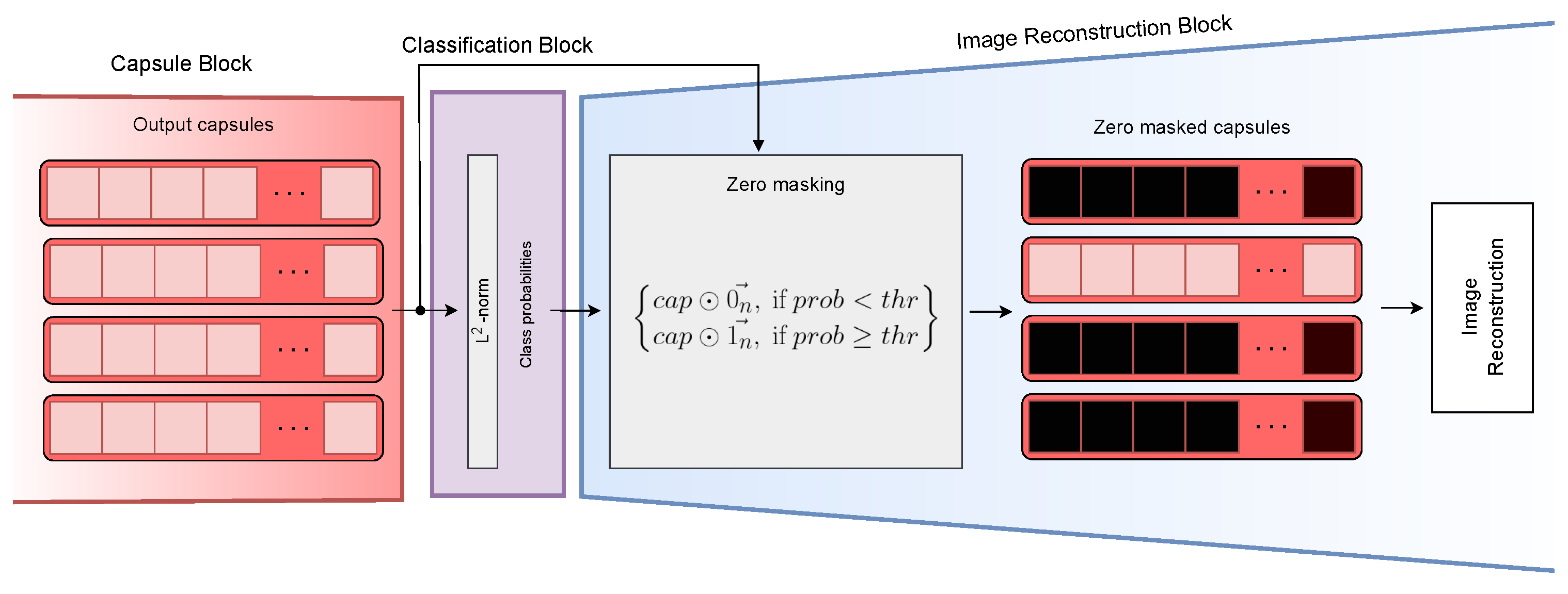
The overall architecture of our proposed network is a combination of ideas from the Efficient-CapsNet from [7] and the original CapsNet from [9] with many small improvements, which we introduced. The schematic representation can be seen in Figure 1. The feature extraction part uses traditional convolutional layers with added BachNormalization and ReLU layers in the feature extraction process [46]. MaxPool layers are also integrated to reduce the number of parameters and capsules [47]. Through stacking multiple convolutional blocks, the extraction of essential features is facilitated, effectively removing unnecessary information and generating a condensed set of capsules. This stacking mechanism enables the model to project the input image onto a higher-dimensional space, thereby facilitating subsequent steps in capsule formation. A key innovation lies in utilizing the same convolutional blocks found in conventional CNNs, allowing for seamless transfer of the feature extraction part and the network’s learned weights to different networks. This approach also enables integration with SOTA models for connecting to subsequent capsule components. The choice of layer and filter quantities is customizable by the user and varies depending on the dataset’s complexity. Simpler datasets need fewer layers and filters, while more intricate datasets require a greater number of layers or filters. Nevertheless, the minimum required number of filters remains smaller than that of traditional convolutional networks.

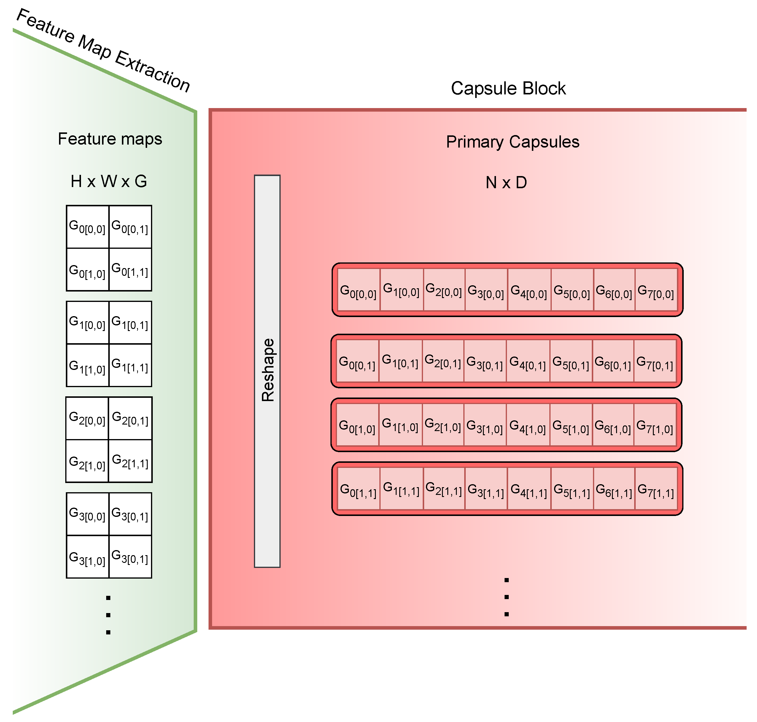
Following the final convolutional block, another convolutional layer is applied, where the output channels are split into multiple capsules the same way as in the original CapsNet, with a small difference in adding the Batchnormalization and ReLU layer, which was added for this experiment. This block produces an output of dimensions $H\times W\times G$, with H representing the height of the transformed image, W denoting the width, and G denoting the number of output channels within the layer. Subsequently, the output is reshaped into primary capsules of size $N\times D$, where N denotes the number of primary capsules and D represents the dimensionality of each capsule. The user determines the number and dimensionality of the primary capsules, ensuring that their product matches the product of the dimensions of the convolutional layer’s output, with G being divisible by D. This reshaping operation serves to create a vector-based representation of the previously extracted features. This operation can be seen in Figure 2.

The introduction of capsules has altered how location information is encoded. In conventional convolutions, location is encoded using a high-value pixel known as place-coded location. However, capsules employ a different approach by encoding location information within vector coordinates. This transformation results in a rate-coded location, compressing the location information into a single numerical value.

CapsNets utilize a dedicated capsule-wise squashing function as the primary activation function within the capsule component of the network. This function serves multiple roles, including introducing non-linearity into the routing process to facilitate learning. Furthermore, the squashing function plays a crucial role in encoding the likelihood of an entity’s presence in the input image by adjusting the length of the capsule. To fulfill this purpose, two conditions must be met. The direction of each capsule should remain unchanged, and the length of the capsule must be confined to the range of zero to one. In this experiment, the squashing function originally proposed in [7] is employed, as depicted in Equation (1). This choice is made due to better sensitivity near zero than the original squash function used in [9]. All equations are in the Einstein notation, so ${{\widehat{u}}^{nm}}_j$ and ${{\widehat{u}}^j}_{nm}$ are the same tensors with the summation performed on the subscript dimension of the first tensor and superscript dimension of the second tensor.

$$v_n=(1-\frac{1}{e^{\left|\right|s_n\left|\right|}})\times \frac{s_n}{\left|\right|s_n\left|\right|},$$

(1)

where $v_n$ is the squashed vector output of one capsule n and $s_n$ is its input. This function satisfies the required properties by returning matrix v with capsules of the same dimensionality and direction as was the input; the only difference is that the lengths of all capsules are squashed into the required interval and non-linearity is introduced into the network to make it more robust.

In CapsNets, routing algorithms play a vital role in transforming raw input data into meaningful representations. The algorithm used in the experiments is based on the original dynamic routing proposed by [9], with multiple improvements. The pseudocode for the algorithm can be seen in

Table 1. Forward pass with routing.

procedure FORWARD(u)	u is a tensor of size $[b,n,i]$
$\widehat{u}\leftarrow$ einsum(’$nmij,bni\to bnmj$’, W, u)	Compute $\widehat{u}$ using Einstein summation convention (Equation (2))
$a\leftarrow$ zeros($[b,n,m]$)	Initialize a with zeros
for  $i\leftarrow 0$  to  $r-1$  do	Perform routing iterations
$c\leftarrow SoftMax\left(a\right)$	Compute c as the $SoftMax$ of a (Equation (3))
$v\leftarrow Squash$(einsum(’$bnm,bnmj\to bmj$’, c, $\widehat{u}$))	Compute v as the squashed sum of $c·\widehat{u}$ (Equation (4))
if  $i<r-1$  then	Update a if not the last iteration
$a\leftarrow$ einsum(’$bmj,bnmj\to bnm$’, v, $\widehat{u}$) $·p$	Update a with intermediate agreement scaled by p (Equation (5))
return  v	Return the final capsule output v

. In the Table and all equations, b is the batch size, n is the number of input capsules, m is the number of output capsules, i is the dimensionality of input capsules, and j is the dimensionality of output capsules. Capsules, which are groups of neurons representing various properties of an entity, rely on routing algorithms to iteratively update their parameters. This process involves first multiplying the input capsules with a weight matrix, which is trained, to obtain the predictions from every input capsule of the pose of each output capsule. This operation essentially learns the transformation from the lower-level features to the higher-level features. Each element of the output tensor $\widehat{u}$ represents the predicted instantiation parameters (such as position, orientation, scale, etc.) of each output capsule, given the input from each lower-level capsule. This multiplication operation can be seen in (2).

$${\widehat{u}}^{nmj}={W^{nmj}}_i\times {u^i}_n,$$

(2)

where ${W^{nmj}}_i$ denotes the weight matrix, ${u^i}_n$ represents the output of the n-th lower-level capsule, and ${\widehat{u}}^{nmj}$ is the prediction for the j-th dimension of the m-th output capsule, based on the n-th input capsule.

After obtaining these predictions, the algorithm iteratively calculates the coupling coefficients to determine the relevance of each lower-level capsule’s output to each higher-level capsule’s output. Initially, the agreements are initialized to zero, and they are then transformed into coupling coefficients using the softmax function along the output capsule dimension, ensuring that the sum of probabilities across all lower-level capsules equals one. This can be seen in (3).

$$c_{nm}=SoftMax\left(a_{nm}\right),$$

(3)

where $c_{nm}$ represents the coupling coefficient between the n-th lower-level capsule and the m-th output capsule, and $a_{nm}$ is the initial agreement initialized as zero.

With the coupling coefficients determined, the algorithm calculates the intermediate and final outputs by combining the predictions from the lower-level capsules weighted by their respective coupling coefficients. This step effectively aggregates information from the lower-level capsules to form the output of each higher-level capsule, which can be seen in (4).

$$v_{mj}=Squash({{\widehat{u}}^{mj}}_n\times {c^n}_m),$$

(4)

where $v_{mj}$ represents the j-th dimension of the output of the m-th capsule, and ${{\widehat{u}}^{mj}}_n$ represents the prediction for the j-th dimension of the m-th output capsule coming from the n-th lower-level capsule, with squash being the function described before in (1).

During each routing iteration, the agreement is updated based on the current predictions and outputs, to improve the coupling coefficients. This is achieved by using only the newly calculated agreement matrix $a_{nm}$ based on the dot product of the output vector and the prediction tensor compared to adding to the previous agreements, as was the case in [9]. An additional small adjustment in this equation was the addition of the learnable parameter p, which behaves as a multiplier on how effective the agreements should be in calculating the coupling coefficients. These adjustments are made to enhance the network’s adaptability to changes in predictions. The operation can be seen in (5).

$$a_{nm}=p\times {v^m}_j\times {{\widehat{u}}^j}_{nm},$$

(5)

where $a_{nm}$ represents the new calculated agreements, ${v^m}_j$ is the intermediate output of capsule m, and ${{\widehat{u}}^j}_{nm}$ is the prediction from the n-th input capsule for the j-th dimension of the m-th output capsule, with p being the added trainable parameter.

Capsule layers can be stacked, and this algorithm remains unchanged, so experiments with multiple capsule topologies can be carried out to reach better performance. The user chooses the number and dimensionality of higher-level capsules, but it is traditional to decrease the number of capsules and increase their dimensionality. This is implemented to reduce the computational complexity for further layers, as the data are more compressed. The number of capsules in the final layer is fixed, as each capsule represents one class from the dataset. An additional capsule can be used, which would not represent any class and would not be used for classification, but it would contain information about the background to help with the reconstruction.

To be able to reconstruct more complicated images from only a few features, the novel idea of this paper was to create a different and more sophisticated architecture. The decoder block selectively masks the outputs of all capsules in the final capsule layer, except for the longest capsule (representing the classification result) or a capsule manually designated for a needed purpose, achieved by element-wise multiplication with a one-hot encoded vector corresponding to the target label. This manual choice approach enables segmentation based on the positive class alone, potentially yielding valuable insights from images classified as negative. Moreover, during training, the true label is consistently designated as the target, rather than the predicted label, to facilitate the training process. The masking operation is shown in Figure 3. The whole layer is then flattened into one vector, which is processed in a fully connected layer and reshaped into a small 2D image with multiple channels. This is a novel approach chosen for CapsNets, which previously used only 1D fully connected layers in the whole decoder for the creation of smaller images. Using multiple blocks of ConvTranspose, Convolutional, and ReLU layers with a decreasing number of channels and increasing size of the images, the new model creates the recreated images in the desired shape. The number and size of these blocks depend on the initial and the desired size of the images. The easiest way to choose them is by mirroring the feature extraction part of the network. The number of output neurons of the fully connected layer would be the same as the total number of inputs for the grouped convolution, which was used in the capsule creation process. The following blocks would then mirror the convolutional blocks backwards to ensure the correct shape of the reconstruction. The final number of channels can differ depending on the target of the reconstruction: three channels for RGB and one channel for greyscale images.

3.1. Classification Loss

The main goal of the CapsNet is accurate image classification. Consequently, the primary and most influential loss is typically the Margin Loss, which is used to train the capsules.

Margin Loss operates similarly to mean squared error (MSE). To make the output of the final capsule layer compatible with MSE, the Euclidean length of the capsules is computed. This transforms the capsule output into a conventional output vector representing probabilities for each class, facilitating the calculation of the total error. The fundamental principle is that the length of a capsule should be close to one if the corresponding entity class is detected in the image, and close to zero otherwise. In contrast to MSE, Margin Loss deals with multiple classes within the same image by computing the loss independently for each class and aggregating the errors. It is calculated using (6).

$$\begin{array}{c}\hfill L_{Margin}=\frac{1}{n}{\sum }_n{y}_n.max(0,m^{+}-\left|\right|v_n{\left|\right|)}^2\\ \hfill +\lambda (1-y_n).max(0,||v_n\left|\right|-m^{-}{)}^2,\end{array}$$

(6)

where $y_n$ corresponds to the label and $v_n$ represents the output capsule for class n. The hyperparameters $m^{+}$, $m^{-}$, and $\lambda$ are used to fine-tune the training process, particularly in the initial phase, to prevent excessive contraction of all capsules, which could impede progress.

To assess the distinctions between different loss functions, the binary cross-entropy (BCE) loss has also been employed as the classification loss, which can be seen in (7). This choice aligns with the conventional usage of this loss function in classification tasks and convolutional networks.

3.2. Reconstruction Loss

Reconstruction plays a fundamental role in most CapsNets, as it enables capsules to learn more generalized information about classes, contributing to the overall concept and improving performance. However, a significant challenge with reconstruction arises when dealing with more complex images beyond the basic Modified National Institute of Standards and Technology (MNIST) dataset [48]. In such cases, capsules require additional information to recreate the input image accurately [9]. Moreover, real-world images often exhibit diverse backgrounds that the network must also learn. The complexity further increases when attempting to reconstruct colored images, as opposed to simpler greyscale images, which can negatively impact performance.

An additional step to decrease the complexity of the reconstruction is to try to segment the object in the image. If the input image is colored, the reconstruction targets can be:

• original coloured image;
• greyscale version of the image;
• segmentation mask (a novel approach for enhancing classification efficiency).

These reconstructed versions are then utilized in the secondary loss, known as the reconstruction loss. Multiple computation methods for this loss exist, but in this experiment, only MSE and BCE losses seen in (7) and (8) are used and compared against their corresponding targets. The MSE is the default loss used in the reconstruction of CapsNets models, and BCE is a loss often used for segmentation. DICE loss and IOU were considered as well, but as they cannot be used for the reconstruction of input images, a comparison could not be made. It should be noted that normalization with mean and standard deviation cannot be applied to BCE, as it would place the targets outside the 0–1 range. The real loss was calculated as a mean of the loss for each pixel value of the original and predicted segmentation mask.

$$\begin{array}{c}\hfill L_{MSE}=\frac{1}{n}{\sum }_n{(x_n-y_n)}^2,\end{array}$$

(7)

$$\begin{array}{c}\hfill L_{BCE}=-\frac{1}{n}{\sum }_n{y}_n.log{x}_n+(1-y_n).log(1-x_n),\end{array}$$

(8)

where $y_n$ is the pixel value of the ground truth mask and $x_n$ is the value of the pixel from the output mask n.

To prevent the reconstruction loss from overpowering the margin loss, a coefficient is introduced, which can be adjusted to observe how the weight of the reconstruction loss influences performance. This scaled loss is then added to the classification loss to obtain the final loss, which is employed for backpropagation seen in (9).

$$\begin{array}{c}\hfill L=L_C+\alpha .L_R\end{array}$$

(9)

where L is the total loss of the model, $L_C$ is the classification loss: either $L_{Margin}$ or $L_{BCE}$ in the case of binary classification, $\alpha$ is the scaling coefficient and $L_R$ is the reconstruction loss: either $L_{MSE}$ or $L_{BCE}$. In certain cases, the introduction of a dedicated capsule solely for reconstruction purposes may be beneficial. This capsule is disregarded during classification and remains unmasked with the others. Its inclusion aids in encoding features and information related to shared background characteristics among classes, thereby improving reconstructions and, consequently, classification performance.

4. Experiments

In this section, we explain the topology of all neural networks used as well as datasets used for the experiments.

4.1. Datasets

For the experiments, two datasets were chosen, both with classification labels as well as segmentation masks. The datasets used for this research were the Oxford-IIIT Pet [49] dataset and the SIIM-ACR Pneumothorax Segmentation dataset, which was based on [50].

4.1.1. Oxford-IIIT Pet

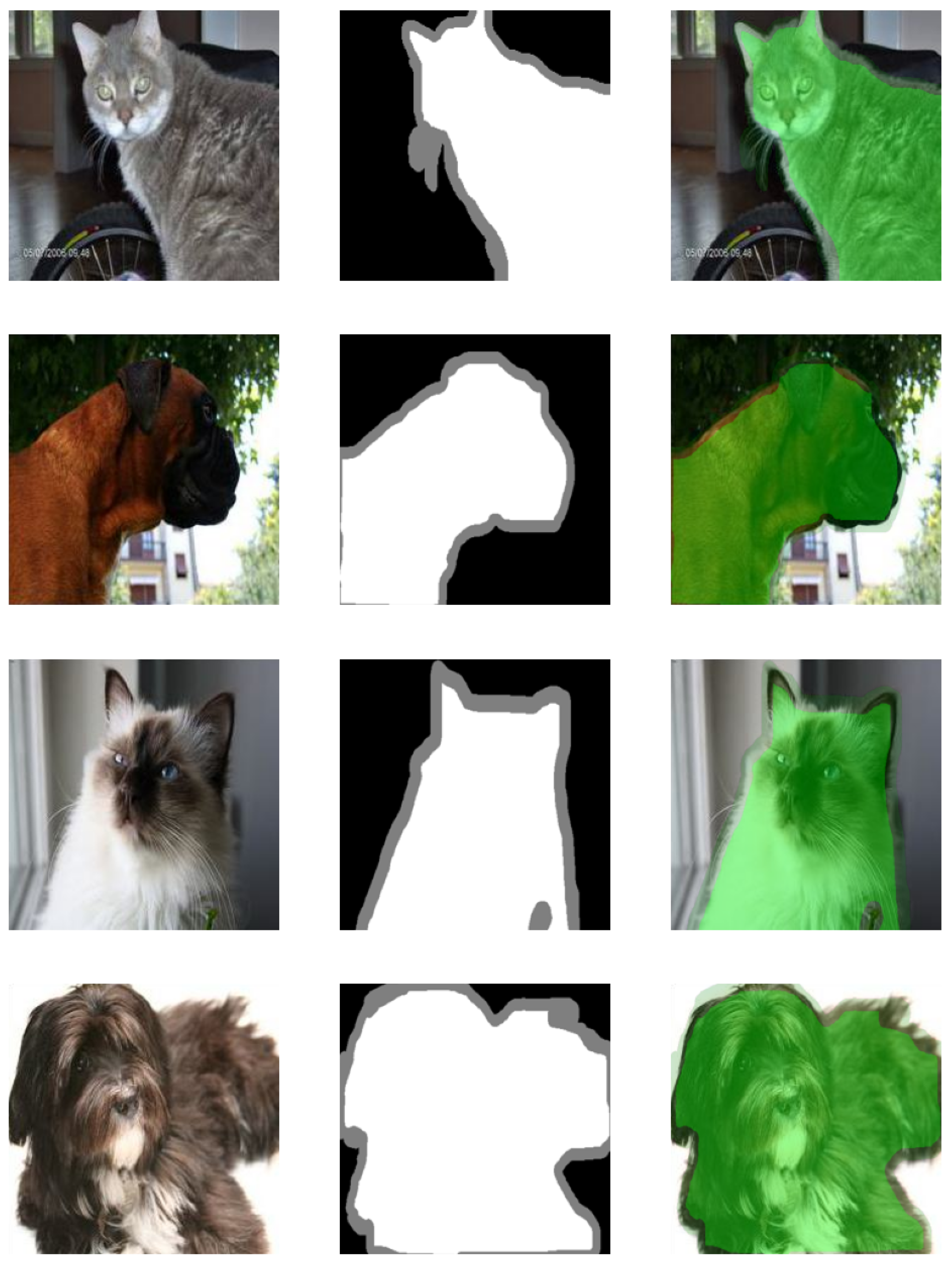
The primary dataset used to test the different methods is Oxford-IIIT Pet [49]. It consists of 4979 images of different breeds of dogs and 2388 images of cats with large variations in scale, pose, and lighting. Examples from this dataset can be seen in Figure 4. Some images were missing the segmentation masks or the masks were empty, so these images were removed beforehand. Although the different breeds were labelled, only the binary classification into cats and dogs was used for this experiment. This dataset was chosen because it represents real-world images much better than the MNIST dataset [48] and other small, simple datasets previously used to test capsules. This choice highlights one of the main disadvantages of capsules: handling images with varied backgrounds. Most images in the dataset have varying dimensions and are not squared. To ensure uniformity and compatibility with the model architecture, these images were resized into squares using the torchvision transform resize function. A square shape of $224\times 224$ pixels was selected for the resized images, balancing computational efficiency and the preservation of image content. While the resized images retain sufficient detail for recognition purposes, they are not overly large, facilitating efficient processing by the network. Using bigger images would be possible with maybe a small increase in performance, but the downside would be the need for larger, slower, and more memory-intensive models.

One significant challenge faced by capsules when working with the Oxford-IIIT Pet dataset is generalizing from highly detailed input images. Detailed images often contain noise and irrelevant features that can distract the model from focusing on the essential aspects needed for accurate classification and reconstruction. This can lead to overfitting, where the model becomes too specialized in recognizing these irrelevant details in the training set, performing poorly on unseen data. The high variability in features present in detailed images, such as differences in lighting, texture, and background elements, makes it difficult for the model to identify the core features relevant to the classification task. The presence of many fine details can overwhelm the model, causing it to focus on minute, non-essential variations rather than the key characteristics that define each class.

Increased computational complexity is also a significant challenge when processing these detailed images. Handling such images requires more computational power and memory, as the model needs to process a larger amount of information. This can lead to longer training times and the necessity for more sophisticated hardware, which might not be feasible in all scenarios. The increased complexity can also make the model more prone to errors and instability during training. These challenges highlight the difficulties in training capsules with highly detailed input images. The high variability in features, risk of overfitting, and increased computational complexity all contribute to making it harder for the model to generalize well from the training data to new, unseen data.

The images in the dataset also come with segmentation masks of the same size, containing three parts: foreground/object, background, and border. The masks are not perfect, as the borders are large and not consistent. To use the segmentation masks and reduce the problem with the border, the masks are converted into arrays with numbers from the interval 0–1; specifically, the background is represented as 0, the border as 0.5, and the foreground as 1. This will ensure that the middle of the object still has the maximum value and that the border around the object is still represented in the output image, but the inaccuracies in the border are not that prevalent in the overall performance. The split into foreground, background, and object was made by the creators of the dataset.

In addition to reshaping the images, a random crop was used. This was added as it showed increased performance in [9]. To ensure that the segmentation masks are cropped in the same way as the input images, after reshaping, all images and segmentation masks are padded by 18 pixels, which creates $242\times 242$ images, and then the top left corner of the cropped image is generated by picking a random point in the top $36\times 36$ square. This square is the same for the input image and the corresponding mask. The final cropped image is taken by obtaining the $224\times 224$ square with the top left corner in the randomly generated point.

The dataset was manually split into training, validation, and test parts with a ratio of 7:1:2. The images used the breed of the pet as the file name with an added number. An easy way to split these images into parts with balanced breeds is by sorting the images alphabetically and adding an index to them. The modulo operation is used with division by 10 on the indices and images, where results equal to 0 and 1 were moved to the test set, those with a remainder of 2 to the validation set, and the rest to the training set.

4.1.2. SIIM-ACR Pneumothorax

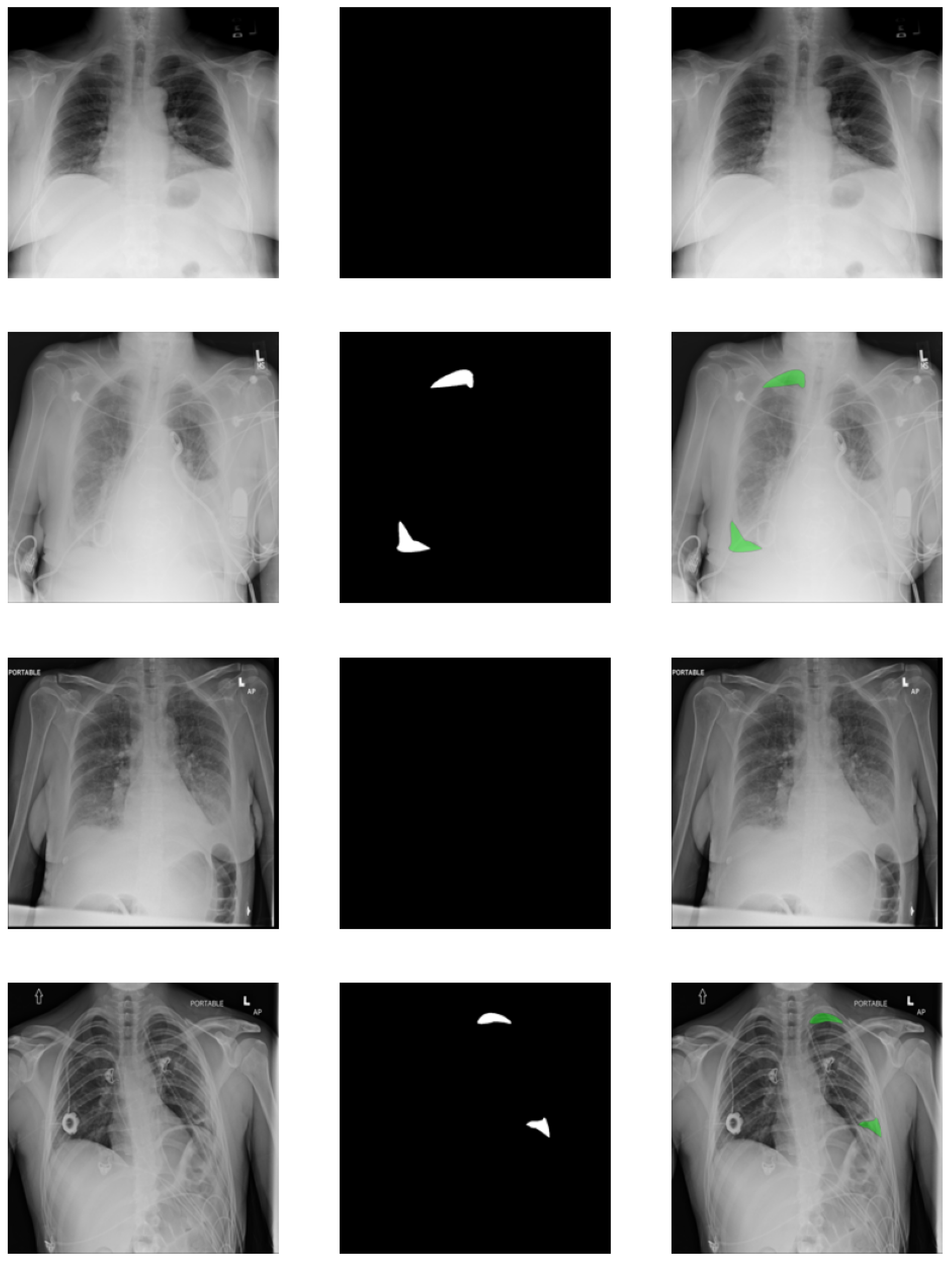
To show that our method works in general, a completely different dataset was selected: SIIM-ACR Pneumothorax containing chest X-rays. This dataset was created for a Kaggle challenge by taking the ChestX-ray14 dataset released by the National Institutes of Health (NIH) [50] and creating pixel-level annotation segmentation masks for images with positive pneumothorax (collapsed lung). The pixel-level annotations were created by the experts specifically for the challenge. Some of the examples can be seen in Figure 5. The final dataset consists of 9378 negative images and 2669 positive images. The size of the original images is $1024\times 1024$, but to simplify the models and speed up training, all were resized to $224\times 224$ to be the same size as images from the first dataset so that the topologies could be identical.

As mentioned before, pixel-level annotations were created for all positive classes. The pixels of the regions containing the signs of pneumothorax are marked with the value 1 and everything else is marked as 0. These were then used as the segmentation masks in the reconstructions. For negative images, an empty array of zeros was used as the target, because there are no traces of pneumothorax anywhere.

The same transformations as in the previous dataset were used: padding and random crop. All masks were resized the same way as the images to have consistently cropped pairs. The split of the dataset was carried out the same way as for Oxford pets with the same split ratio of 7:1:2 between training, validation, and test sets.

4.2. Network Structures

The first network used in the experiments is created from the concepts of the original CapsNet from [9]. This network was slightly modified to work with bigger images and a smaller number of classes. The reconstruction part of the network is modified as well to work with 2D color images and is the same as other capsule decoders in this paper, but the implementations of the routing algorithm and other parts of the network are the same as the original. Even though the architecture is slightly changed and no fine-tuning was performed, this network will be further called the original CapsNet.

As our created network used ideas from [7], this network has been used for benchmarking as well. We modified the network from the paper slightly to work with bigger images. The one bigger change was in the squash function, as the squash function used in this paper was unable to train properly with our learning rates, so the squash function from the original CapsNet was used.

The model from [29] was chosen as an additional capsule benchmark. The base of the topology was the same as the one in the original paper with the only difference being the hyperparameters, which were $A=32$, $B=8$, $C=8$, $D=8$, $K=3$, $P=4$, and iters $=3$. This was done because of the limited amount of GPU memory available for experiments. The network is not using reconstruction.

For the main network in the experiment, several variations of C-CapsNet, described in Section 3, were used. The differences between the variations were in the type of reconstructions, the reconstruction loss used, the classification loss used, and the use of the background capsule for easier reconstruction.

The topology of the feature extraction part was the same for all capsule models; the first convolutional block used a $5\times 5$ kernel and its output had 16 channels. All other convolutional blocks used a kernel of size $3\times 3$ and output channels of size 16, 32, 64, and 128, in that order. The primary capsule layer of the Efficient-CapsNet used a kernel of size 3 and returned 72 capsules with a dimensionality of 16. The original CapsNet and our network used 288 output channels to obtain the same sizes for capsules. The padding used in all convolutional layers was set to valid. Two routing layers were used, which transformed $72\times 16D$ capsules into $8\times 16D$ and finally into $2\times 28D$ capsules. For models with additional capsules for the background, the output of the last routing layer was $3\times 28D$ capsules. It can be seen in

Table 2. The structure of the feature extractor with output dimensions (BatchNorm and ReLU layers are not mentioned, but used after every MaxPool).

Layer	Input	Channels	kernel	Output
Conv	224	16	5	220
MaxPool	220	16	2	110
Conv	110	16	3	108
MaxPool	108	16	2	54
Conv	54	32	3	52
MaxPool	52	32	2	26
Conv	26	64	3	24
MaxPool	24	64	2	12
Conv	12	128	3	10
MaxPool	10	128	2	5

. The feature extraction part was specifically designed to be used with the input of size $224\times 224$, but by adding or removing layers, the network should be able to handle any input size and ratio.

The reconstruction part of the network was composed of one dense layer and four ConvTranspose blocks. The output of capsules from the final routing layer is masked and then flattened, which will create 56 or 84 neurons in the case of a background capsule. These are then used in a fully connected layer with 1452 neurons as output, which can be reshaped into the shape of $12\times 11\times 11$. The ConvTranspose layer is always using the same number for input and output channels, kernel size of 5 and stride 2. The differences are in the padding of input and output. Convolutional layers use the ’same’ padding and a kernel of size 3, with a different number of output channels. The first block uses an output padding of 1 and outputs 10 channels, the second uses no padding and outputs 8 channels, the third uses an input padding of 1 and outputs 8 channels, and the final block uses both input and output padding of 1 with output channels of 1 or 3 depending on the target of reconstruction. The sigmoid activation function is used instead of ReLU in the final step. The reconstruction was also specifically designed to return images of size $224\times 224$, but with the changes of the padding and the number of layers, other image sizes and ratios are possible. To have some benchmark for a traditional convolutional network, a simple CNN consisting of five convolutional blocks, each with BatchNorm, ReLU, and MaxPool2d layers, was used; these were the same blocks used in the CapsNets. The classification part of the network consists of two linear layers. The size of each layer was chosen to have a comparable number of parameters and sizes of convolutions to the used CapsNets. Two additional CNNs were created with different numbers of channels and convolutional layers to try to maximize the performance available from CNNs, one with five and the other with six convolutional blocks in total.

The baseline CNN topology is similar to CapsNets in the feature extraction part with the same number of convolutional layers, channels, and kernels. The classification part is created using two linear layers, where 3200 neurons are first transformed into 256 neurons and then into the final 2 neurons for each class. Between these layers, 1D batch normalization, dropout, and ReLU layers are used. The differences with the other CNNs are in the number of convolutional blocks, channels, and the first fully connected layer. By using 64 output channels from the fifth block, the number of flattened features of the linear layer is changed to 1600 and the output to 128 neurons. The addition of the sixth convolution block reduces the size of the linear layer to 256 and it has an output size of 128 neurons. The network with the same feature extraction part as CapsNets is called Bigger CNN, the one using 64 output channels and 1600 neurons in the first fully connected layers is called Smaller CNN, and finally, the CNN with six convolutional blocks is called 6block CNN.

4.3. Setup

The training of all capsule models was carried out for 200 epochs and 100 epochs for convolutional models both with a batch size of 256. For models using EMRouting, the base was the batch size, limited to 6, as it used more GPU memory than the others. The experiments were coded using the PyTorch framework [51] with its package Torchvision for custom data loaders capable of returning inputs, labels, and segmentation masks in one function. The training was carriedout on an RTX 4090 with 24 GB of memory and 128 GB of RAM. The only optimizer used was Adam [52] for all models. As both datasets are highly imbalanced, a custom sampler was used, which ensured a balanced picking of images from each class during training.

For each capsule topology, two classification losses, two reconstruction losses, the inclusion or exclusion of a background capsule, and the selection from three distinct reconstruction targets are considered, resulting in a total of 24 unique configurations tested in the experiments.

A range of initial learning rates was used to find the one with the best performance. The final chosen learning rate for all CapsNets was 0.002, and for the benchmark CNNs, it was 0.001. Learning rate decay was also used in all models with a gamma of 0.98 and a step after each epoch. The values of hyperparameters $m^{+}$, $m^{-}$, and $\lambda$ are 0.9, 0.1, and 0.5 in these experiments, keeping the same values as the original implementation in [9]. For each configuration of a model, four experimental runs were conducted with random initial parameters. Mean and standard deviation were calculated to ensure that the performance of the model in one specific run was not a rare occurrence. The final performance of each model is calculated by saving the parameters of the epoch with the best validation performance (lowest validation classification loss) and parameters from the end of the training after all epochs. These weights were then tested on the test set and the maximal performance was taken and recorded.

5. Results

We compared multiple models with variations in their classification and reconstruction loss functions, usage of background capsules, and most important for these experiments, the type of reconstruction on the described datasets to show that our implementation can obtain better results than the previous works. For almost all capsule models, the weights at the end of the training were recorded, as they performed better than those taken from the moment of the lowest validation loss, and for almost all convolutional models, the exact opposite was true.

5.1. Results on Oxford Pets

For the evaluation of models on this dataset, the macro-F1 score was used as a performance metric, as the dataset does not have one positive class [53]. The configurations of the models with the best performance from each reconstruction target and model type can be seen in

Table 3. The best-performing configurations for each type of model and reconstruction target used for the Oxford Pets dataset.

Model Type	Recon Target	Recon Loss	Class Loss	Bg Capsule
C-CapsNet	RGB	MSE	margin	No
C-CapsNet	GS	MSE	margin	No
C-CapsNet	mask	BCE	margin	Yes
Original	RGB	BCE	margin	Yes
Original	GS	MSE	margin	No
Original	mask	BCE	cross-entropy	Yes
Efficient	RGB	BCE	margin	Yes
Efficient	GS	BCE	margin	No
Efficient	mask	MSE	margin	Yes

. The performances of all models can be seen in

Table 4. The average performances of the models used in our Oxford Pets experiments with added time per epoch and a number of parameters. In bold is our best-performing model without counting SOTA.

Model Type	Recon Target	Time per Epoch (s)	Number of Parameters	F1-Score (%)
C-CapsNet	RGB	3.7	682K	${92.72}_{\pm 0.14}$
C-CapsNet	GS	3.9	682K	${93.04}_{\pm 1.03}$
C-CapsNet	mask	6.4	726K	${\mathbf{93.39}}_{\pm \mathbf{0.66}}$
Original	RGB	4.0	726K	${92.77}_{\pm 0.91}$
Original	GS	3.9	681K	${92.44}_{\pm 0.81}$
Original	mask	6.3	726K	${93.16}_{\pm 0.05}$
Efficient	RGB	3.9	395K	${92.47}_{\pm 0.28}$
Efficient	GS	3.7	351K	${92.10}_{\pm 0.53}$
Efficient	mask	6.5	395K	${92.82}_{\pm 0.86}$
EMRouting	-	622	26K	${65.54}_{\pm 4.32}$
Smaller CNN	-	3.4	268K	${89.53}_{\pm 1.04}$
Bigger CNN	-	3.5	920K	${90.73}_{\pm 0.53}$
6block CNN	-	3.5	429K	${89.85}_{\pm 0.75}$
TWIST [54]	-	10	25M	$94.5$

.

All versions of models reached the best classification performance using the $\alpha$ coefficient of 0.3 for both reconstruction losses. As can be seen in Table 3, the best-performing models mostly use margin loss as the one with better performance, with the only exception being the original CapsNet using segmentation masks. The performances of the best overall trained models can be seen in Table 4. The use of BCE and MSE loss and the use of background capsules have not given any noticeable advantage in the results. As can be seen in Table 4, the best-performing model is our improved CapsNet, reconstructing segmentation masks with 93.39%, with other capsule models reconstructing masks being close behind, with 93.16% and 92.82%. CNN models only reached a performance of about 90%, while the EMRouting model was unable to reach more than 66%. The SOTA algorithm TWIST used pre-trained RESNET-50 [55] as a backbone and reached the best accuracy of 94.5%, which is better than our models, but the non-pre-trained version reached an accuracy of only 91.6% [54], which is less than the capsule models, and the computational time is almost double.

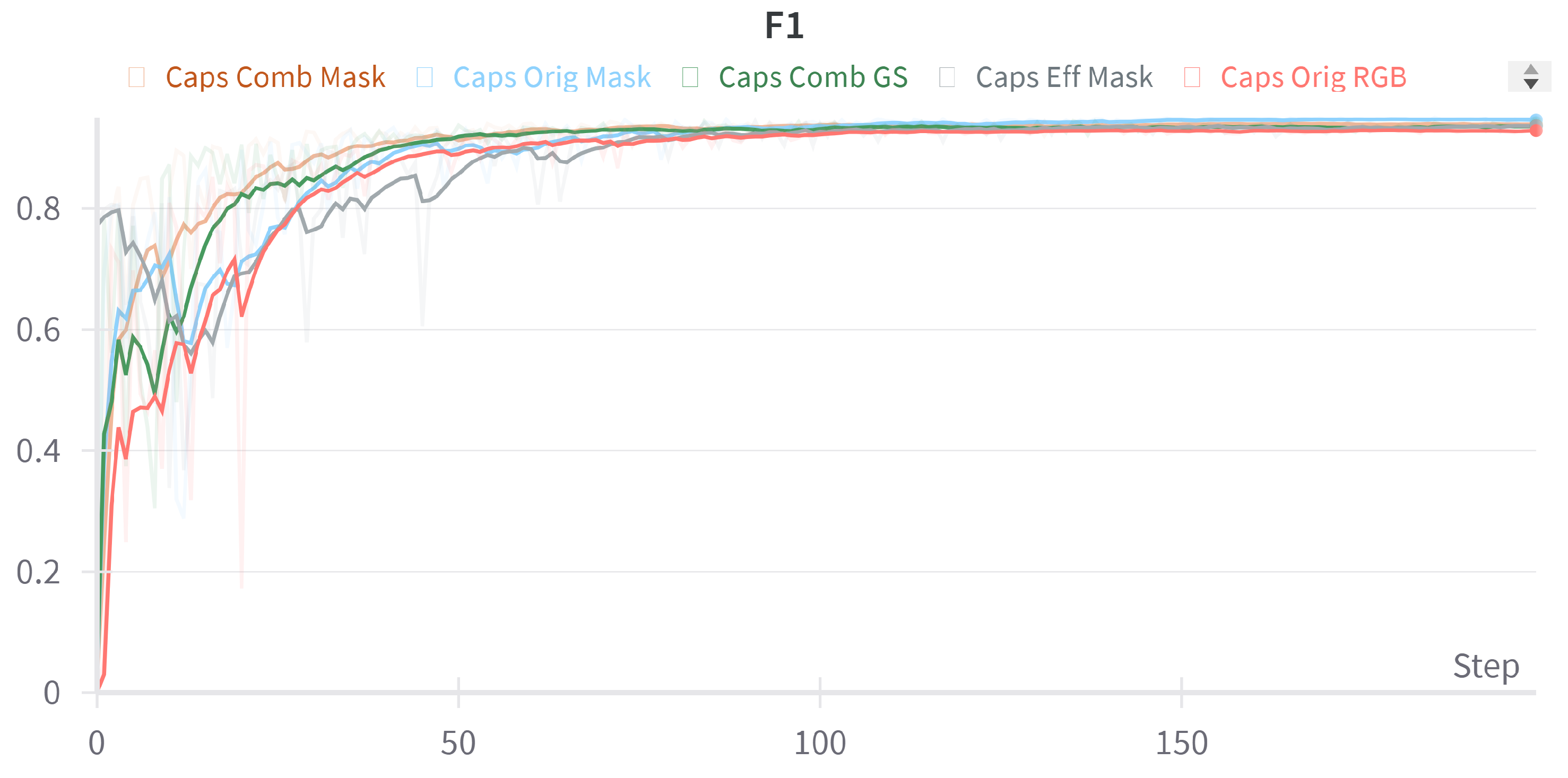
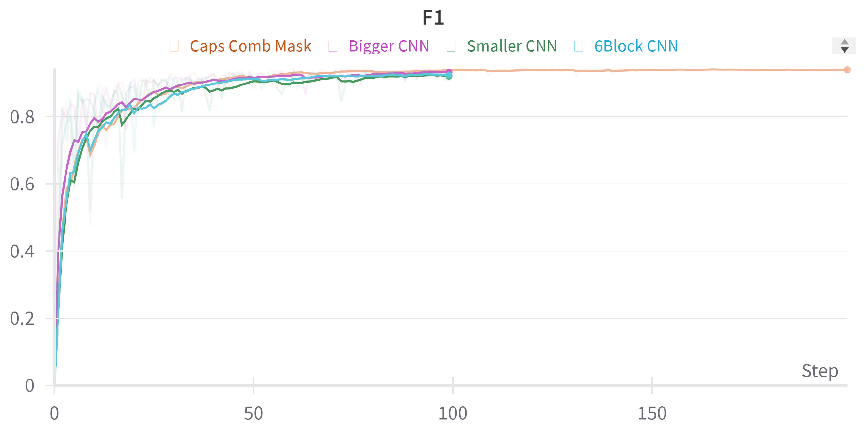
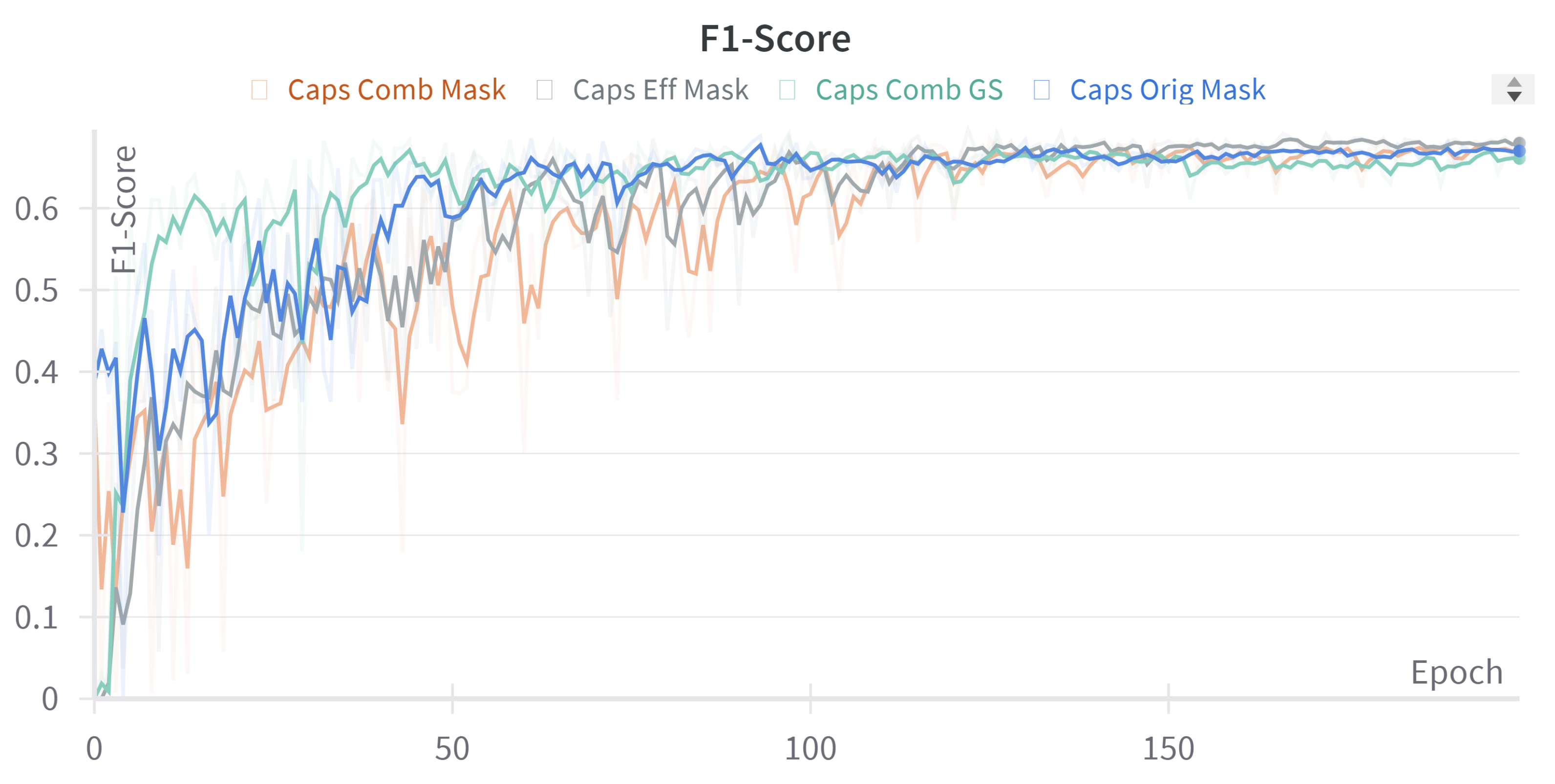
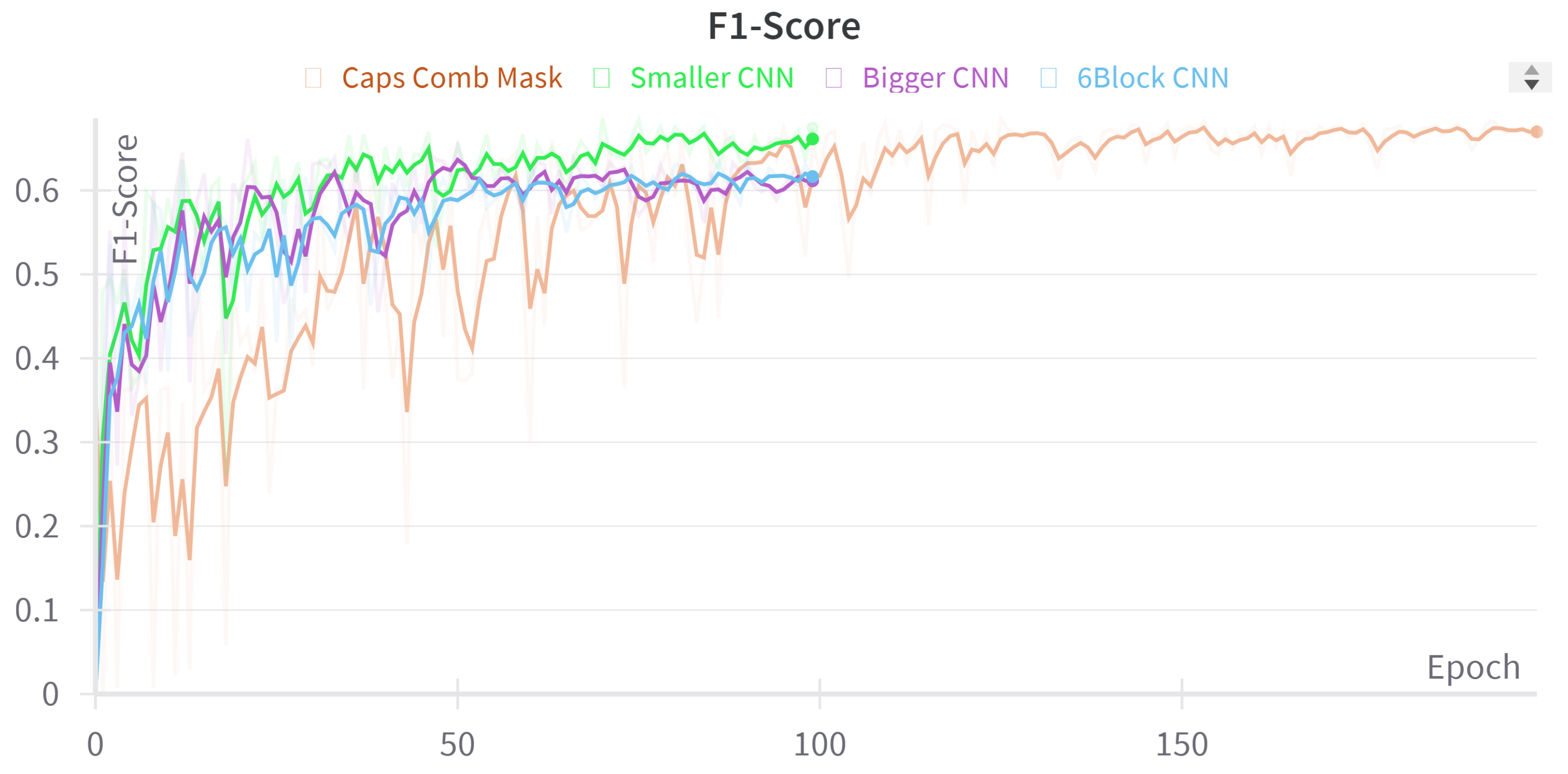
Figure 6 and Figure 7 show the validation F1 score of selected representative models during their training period. F1 score is selected as comparing losses is almost impossible when different loss functions are used. The main lines are created using a smoothing function to see the trends of the training, as having an imbalanced dataset creates large peaks during the training, which can still be seen as a shadow in the figure.

To show how the reconstruction works, the C-CapsNet models with the best F1 score were used to recreate several images from the test dataset. One example can be seen in Figure 8, where the top left image is the original image, the top right is the reconstruction output of the best-performing model with colored reconstruction, the bottom left one is the output of the greyscale model, and finally, the bottom right is the output of the segmentation model. The results on other images from the dataset were similar.

5.2. Results on SIIM-ACR Pneumothorax

We compared the same topologies using the second dataset. The best accuracy of all models was around 84%, but as a highly imbalanced medical dataset was used, there is a need to use different performance metrics. Because of that, for this experiment, the F1-score is chosen as the main performance metric, as it considers both the precision and recall score, which was needed to ignore the number of true negative images. The best-performing models from each capsule category can be seen in

Table 5. The best-performing configurations for each type of model and reconstruction target used for the SIIM-ACR Pneumothorax dataset. As the original images were in greyscale, no RGB target of reconstruction is used.

Model Type	Recon Target	Recon Loss	Class Loss	Bg Capsule
C-CapsNet	GS	BCE	cross-entropy	No
C-CapsNet	mask	BCE	cross-entropy	No
Original	GS	BCE	cross-entropy	No
Original	mask	BCE	cross-entropy	Yes
Efficient	GS	BCE	margin	Yes
Efficient	mask	BCE	margin	Yes

.

All models used the same $\alpha$ coefficient as in the first dataset: 0.3. From

Table 6. The average performances of the models used in medical experiments with added time per epoch and a number of parameters. In bold is our best-performing model.

Model Type	Recon Target	Time per Epoch (s)	Number of Parameters	F1-Score (%)
C-CapsNet	GS	5.3	681K	${66.72}_{\pm 0.53}$
C-CapsNet	mask	6.3	681	${\mathbf{67.02}}_{\pm \mathbf{0.79}}$
Original	GS	5.3	680K	${66.30}_{\pm 1.42}$
Original	mask	6.5	725K	${66.43}_{\pm 0.79}$
Efficient	GS	5.5	395K	${66.68}_{\pm 1.06}$
Efficient	mask	6.7	395K	${66.92}_{\pm 0.28}$
EMRouting	-	971	24K	${9.16}_{\pm 18.31}$
Smaller CNN	-	3.4	268K	${65.13}_{\pm 1.80}$
Bigger CNN	-	3.5	920K	${63.35}_{\pm 2.76}$
6block CNN	-	3.5	429K	${62.37}_{\pm 1.05}$
RESNET-50 [55]	-	15	25M	${66.48}_{\pm 0.51}$

, we can see that the medical images are harder to classify than the Oxford Pets dataset and the models are unable to reach performance, which would be satisfactory for the doctors. The final results had a slightly better recall percentage than the precision, at around 80%, which is the better of the two cases. By using the segmentation masks as the reconstruction targets, the F1-scores of around 67% are seen using BCE loss. For this dataset, models using MSE loss for reconstruction were performing worse than their BCE counterparts. The models using cross-entropy loss for classification reached better performances than those using margin loss, with the exception being Efficient CapsNet. The model using EMRouting was even worse compared to the other models, as it only reached an F1-score of 9.16%, which was mostly guessing the same label for everything or making completely random guesses. The smaller five-block CNN reached the best performance of the CNN models, with a mean F1-score of 65.13%, with others reaching 63.3% and 62.3%. Background capsules were used in all models, which had segmentation masks input as reconstruction targets, but only in one case when the original image was the target. From our research, the dataset was only used for segmentation, not classification, so no SOTA results could be found for the classification performance, but using pre-trained RESNET-50 as a good benchmark, the model reached an F1 score of 66.48%, which is close to the best capsule model. Still, it uses different data for pre-training and the time is almost triple the best model.

The training of the networks seen in Figure 9 shows how close the performance of our CapsNets with the segmentation mask and the input image is. However, as seen in Figure 10, even though CNNs have better performance at the beginning, they will reach their peak performance much sooner, which enables the CapsNet to catch up and overtake them towards the end of the training.

In addition to the classification, C-CapsNet models generate reconstructions of the specified targets. Several examples of these can be seen in Figure 11. The first column shows the input images for all models, the second the output of the best-performing original image reconstruction model, the third column shows the segmentation masks of these images, and the final column shows the outputs of the best-performing segmentation reconstruction model. These four examples were chosen, as they best represent the usual cases on other data. The false negative images have no segmentation and the false positive have random regions highlighted.

6. Discussion

Based on the results presented in the previous section, several general observations can be made. The difference in model performance between those using the background capsule and those that do not is significant only when the input images share many similar aspects, which are then saved in the shared capsule, while the differences between classes are saved in other capsules. However, this distinction is less prominent in the Oxford Pets dataset, where backgrounds vary greatly, even between classes. Models using segmentation masks experience small but consistent performance gains as the compositions of scenes with masks of different classes have many similarities, and the class capsules are only used for accurate reconstruction of specific shapes of different breeds.

The CapsNet models using EMRouting perform poorly on large and complex images. This limitation is a general drawback of EMRouting models due to the limited scalability of this topology and the high GPU memory requirements for effective training. The original CapsNet implementation performs well on the Oxford Pets dataset, while the implementation of Efficient CapsNet performs better on the SIIM-ACR Pneumothorax dataset, but the best overall performance is achieved by using our improved network, which reached the best results on both datasets. The use of segmentation masks as reconstruction targets shows an improvement in performance on both datasets, with an increase of 0.5% and 0.3%, respectively. This is not that statistically significant, but still the gain is shown to be general. Although the difference between greyscale and color images as targets is small, different models achieve better classification performance using different targets. This phenomenon may be attributed to how background information is stored in the capsules of each topology, which can make the recreations easier for the specific implementation.

From the results on both datasets, it is evident that the variability of image backgrounds does not have a straightforward correlation with the performance of the segmentation-based reconstruction method. This observation is supported by the proportional performance improvement achieved by using segmentation masks across both datasets, despite the significantly different background variability in each dataset. However, the quality and consistency of the segmentation masks used can cause multiple issues. If the segmentation masks are completely incorrect, the model may learn information from the wrong regions, hindering classification performance, as the class capsule should contain the features for segmentation. Similar problems arise if there are inconsistencies in the masks or inaccuracies in the boundaries. These errors can mislead the model, causing it to focus on irrelevant or incorrect features, ultimately reducing the effectiveness and accuracy of the classification process. Therefore, ensuring the accuracy and consistency of segmentation masks is crucial for optimal model performance [56].

Compared to traditional CNNs of various sizes, our capsule model achieves better peak performance with similar or smaller standard deviations, with an average difference of 3% and 2.5%, respectively. Although the differences between convolutional networks are minimal, models with more parameters show a slight improvement in the first dataset. To achieve the performance level of our C-CapsNet, a CNN would need approximately 20 million parameters, based on the observed performance increase when transitioning from 64 to 128 channels in the last block of the first dataset. This is evident in the SOTA performance of the TWIST method, which achieved its best results with 25 million parameters. However, for the Pneumothorax dataset, increasing the number of parameters does not improve the performance of convolutional models; in fact, it worsens it. This deterioration is likely because the additional filters capture variations not present in lung images, leading to overfitting. Although using a pre-trained RESNET model helps, our C-CapsNet model still outperforms it when using a segmentation mask as the reconstruction target.

The less conclusive results on the SIIM-ACR Pneumothorax dataset compared to the Oxford Pets dataset may be attributed to several factors inherent to the nature and challenges of medical image analysis. First, the variability and subtlety of features in medical images make it inherently more difficult to achieve high classification accuracy. Pneumothorax, being a condition that can present with very subtle visual cues, poses a significant challenge even for experienced radiologists. Consequently, the model may primarily learn the main differences between clearly positive and negative images but struggle with those that are less distinct.

The choice of a better general reconstruction loss depends on the dataset. Models using MSE loss achieved the same performance on the Oxford Pets dataset, with a maximum difference of 0.3%, while BCE loss proved superior for both reconstruction tasks and helped outperform other models on the SIIM-ACR dataset with an average increase of 1%.

When considering the classification loss function, the one that consistently yields better performance is not definitively clear. On the Oxford Pets dataset, the average performance difference between models trained with margin loss and cross-entropy loss was 1%, indicating that margin loss tends to be superior for similar datasets. However, on the pneumothorax datasets, the results were nearly reversed, with cross-entropy loss exhibiting an average improvement of 0.4% across all models except Efficient CapsNet. Nevertheless, it can be concluded that when utilizing Efficient CapsNet, margin loss consistently outperforms other approaches.

Training time for models within the same category is similar across datasets, with minimal differences. CNN models exhibit the shortest training time due to the simpler complexity of the fully connected layer compared to the routing algorithm. The longer training time of the CapsNet implementations is attributed to the complexity of the routing process, which takes more time than using simple fully connected layers. The increase in time for the models using segmentation masks as the targets is caused by the need to read the additional masks from memory and do more transformations, which will slow down the loading of data. The EMRouting model’s lengthy training time is a result of the algorithm’s poor scalability for larger images.

The performance progress across epochs differs between capsule models and CNNs. Capsule models exhibit a slower start but eventually surpass convolutional models in performance. This can be attributed to the more complex nature of training capsules, as they need to learn connections of features in an additional dimension and require multiple passes over the dataset to achieve the desired generalization. In contrast, training fully connected layers in CNNs, which operate in one dimension, can be accomplished in fewer epochs. However as the structure is simpler, the CNNs are not able to reach the performance of capsules.

Reconstruction results shown in Figure 8 and Figure 11 vary greatly for each dataset, with capsules struggling to learn and generalize colors of smaller image parts, often resorting to the average color as the main hue for recreations in the colored reconstructions of the first dataset. Differences between greyscale and colored reconstructions are not apparent, except for minor discrepancies in the shape and length of the ears. The overall shape of the cat is visible, but finer details cannot be recognized. Segmentation masks show promise, as the placement and rotation of the cat are correct, although the shape of the ears and body appear wider than in the original image.

For the second dataset, input image reconstructions are better than those from the Oxford Pets dataset due to lower variability in overall shape and the absence of background. While some details are lost, they are not crucial for the overall classification process. However, all reconstructions capture the shape, size, and location of the lungs, which are important for pneumothorax detection.

The quality of segmentation reconstructions depends on the specific input image. In most cases, the placement of segmented regions is correct, with various deformations applied. However, some images only segment a single part or provide entirely incorrect segmentations. This issue also arises in incorrectly classified images when the wrong capsule is used for reconstruction.

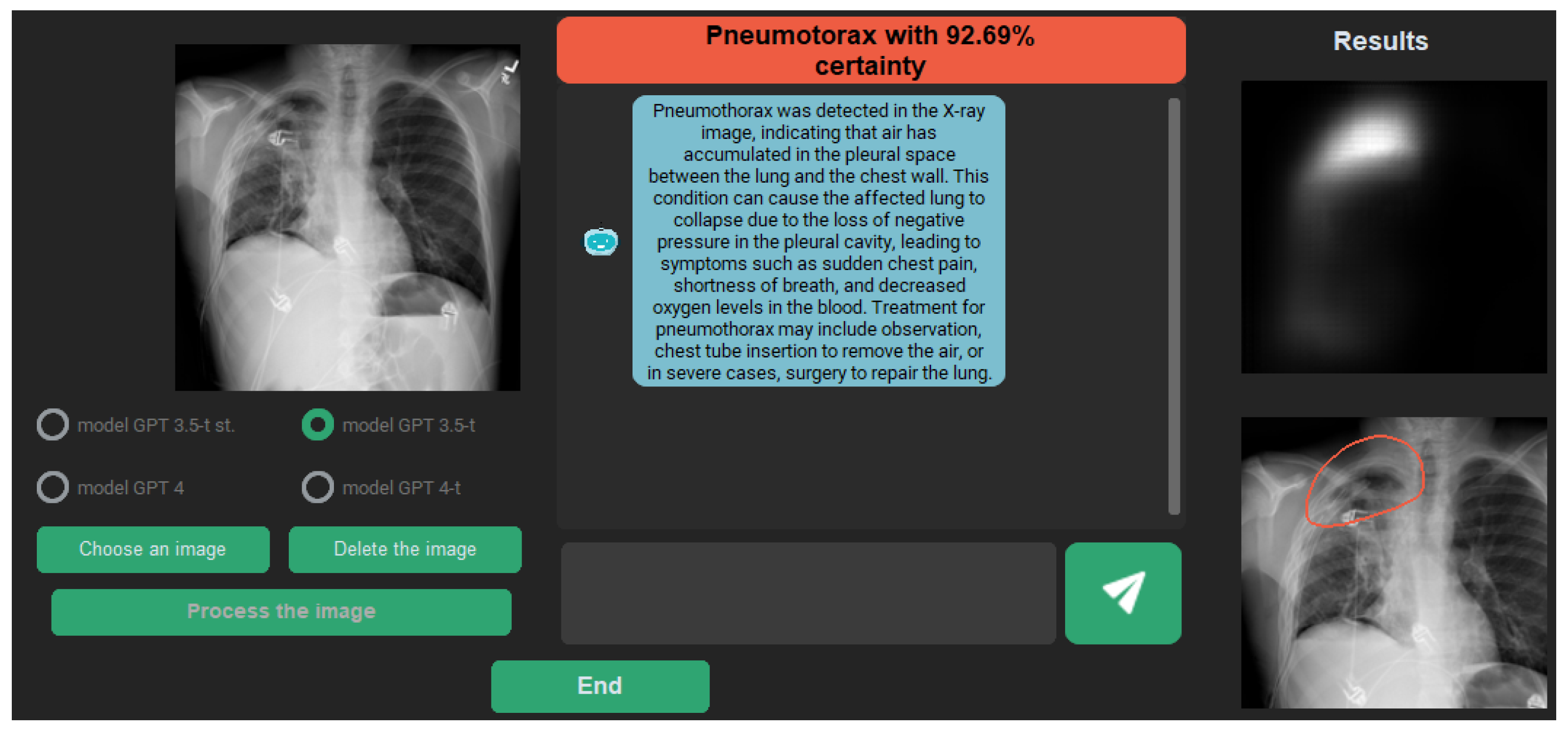
Reconstructions provide insight into what our model requires for accurate classification, aiding model explainability. Doctors can identify regions highlighted by the model as collapsed areas and focus on confirming the classification result. With time, this can lead to increased trust in the model, enabling more autonomous use and speeding up the diagnostic process by avoiding numerous negative images. With slight modifications, this approach can be used as an explanation module, taking an X-ray image as input and returning a diagnosis with identified regions for positive cases. Adding textual information to provide details such as severity and other useful information could further improve the module.

One possible explanation module prototype can be seen in Figure 12, which uses the classification output of the network and the segmentation map as a prompt for Chat-GPT. Chat-GPT then takes the role of the doctor and describes the detected illness with the possibility of communicating further to ask more questions about what to do with this information and how to get better.

7. Conclusions

In this study, we present a modified CapsNet architecture called C-CapsNet, which combines elements from Efficient-CapsNet and the original CapsNet, while incorporating segmentation masks as reconstruction targets. By using segmentation masks for reconstructions, the models can effectively generalize the essential information required for accurate reconstruction, leading to improved performance. However, generalizing information from fully detailed input images poses significant challenges for our models. Through comprehensive evaluations on two diverse datasets, we demonstrate that utilizing segmentation masks enhances model performance in classification, surpassing other capsule and convolutional models.

Our findings indicate that the BCE loss function yields superior results for reconstruction, even when reconstructing original images. The best-performing C-CapsNet model achieved a mean F1 score of 93% on the Oxford Pets dataset while reaching the final F1 score of 67% on the SIIM-ACR PNEUMOTHORAX dataset. Different CapsNet implementations can be used for different datasets, as no superior implementation can be found in our experiments. The performance of CapsNet models can be increased by using segmentation masks. Furthermore, these models offer potential applications in enhancing explainability and fostering trust among medical professionals and other users by creating images capable of showcasing the exact regions the models are looking at during their diagnosis.

Future investigations will explore more intricate reconstruction topologies, incorporating skipped connections to leverage the benefits observed in traditional U-Net architectures. Additionally, we will explore an alternative reconstruction target, namely the original input image multiplied by the mask, which could facilitate improved generalization by downplaying the significance of the background. Moreover, we will consider employing the Dice loss as the primary reconstruction loss metric.

However, our approach entails certain limitations. Firstly, it relies on the availability of training datasets that contain both classification labels and corresponding segmentation masks. Given the scarcity of such datasets, the widespread adoption of this method may be hindered. Additionally, the performance of the network, although superior to other methods, is not yet at a level suitable for clinical use. Mitigating this limitation could involve leveraging pre-trained feature extractors and incorporating more extensive datasets to improve overall performance.

References

1. Krizhevsky, A.; Sutskever, I.; Hinton, G.E. Imagenet classification with deep convolutional neural networks. Commun. ACM 2017, 60, 84–90. [Google Scholar] [CrossRef]
2. Belongie, S.; Carson, C.; Greenspan, H.; Malik, J. Color-and texture-based image segmentation using EM and its application to content-based image retrieval. In Proceedings of the 6th International Conference on Computer Vision (IEEE Cat. No. 98CH36271), Bombay, India, 7 January 1998; pp. 675–682. [Google Scholar]
3. Specht, D.F. A general regression neural network. IEEE Trans. Neural Netw. 1991, 2, 568–576. [Google Scholar] [CrossRef] [PubMed]
4. Abdelhamid, A.A.; El-Kenawy, E.S.M.; Alotaibi, B.; Amer, G.M.; Abdelkader, M.Y.; Ibrahim, A.; Eid, M.M. Robust speech emotion recognition using CNN+ LSTM based on stochastic fractal search optimization algorithm. IEEE Access 2022, 10, 49265–49284. [Google Scholar] [CrossRef]
5. Lopac, N.; Hržić, F.; Vuksanović, I.P.; Lerga, J. Detection of Non-Stationary GW Signals in High Noise From Cohen’s Class of Time–Frequency Representations Using Deep Learning. IEEE Access 2021, 10, 2408–2428. [Google Scholar] [CrossRef]
6. Jaiswal, A.; AbdAlmageed, W.; Wu, Y.; Natarajan, P. Capsulegan: Generative adversarial capsule network. In Proceedings of the European Conference on Computer Vision (ECCV) Workshops, Munich, Germany, 8–14 September 2018; pp. 526–535. [Google Scholar]
7. Mazzia, V.; Salvetti, F.; Chiaberge, M. Efficient-capsnet: Capsule network with self-attention routing. Sci. Rep. 2021, 11, 14634. [Google Scholar] [CrossRef] [PubMed]
8. Hinton, G.E.; Krizhevsky, A.; Wang, S.D. Transforming auto-encoders. In Proceedings of the International Conference on Artificial Neural Networks, Espoo, Finland, 14–17 June 2011; Springer: Berlin/Heidelberg, Germany, 2011; pp. 44–51. [Google Scholar]
9. Sabour, S.; Frosst, N.; Hinton, G.E. Dynamic routing between capsules. Adv. Neural Inf. Process. Syst. 2017, 30, 3856–3866. [Google Scholar]
10. Ribeiro, F.D.S.; Leontidis, G.; Kollias, S. Capsule routing via variational bayes. In Proceedings of the AAAI Conference on Artificial Intelligence, New York, NY, USA, 7–12 February 2020; Volume 34, pp. 3749–3756. [Google Scholar]
11. Wang, W.; Lee, F.; Yang, S.; Chen, Q. An improved capsule network based on capsule filter routing. IEEE Access 2021, 9, 109374–109383. [Google Scholar] [CrossRef]
12. Haq, M.U.; Sethi, M.A.J.; Rehman, A.U. Capsule Network with Its Limitation, Modification, and Applications—A Survey. Mach. Learn. Knowl. Extr. 2023, 5, 891–921. [Google Scholar] [CrossRef]
13. Xi, E.; Bing, S.; Jin, Y. Capsule network performance on complex data. arXiv 2017, arXiv:1712.03480. [Google Scholar]
14. Patrick, M.K.; Adekoya, A.F.; Mighty, A.A.; Edward, B.Y. Capsule networks–a survey. J. King Saud-Univ.-Comput. Inf. Sci. 2022, 34, 1295–1310. [Google Scholar]
15. Wang, Y.; Huang, L.; Jiang, S.; Wang, Y.; Zou, J.; Fu, H.; Yang, S. Capsule networks showed excellent performance in the classification of hERG blockers/nonblockers. Front. Pharmacol. 2020, 10, 1631. [Google Scholar] [CrossRef] [PubMed]
16. Xiang, C.; Zhang, L.; Tang, Y.; Zou, W.; Xu, C. MS-CapsNet: A novel multi-scale capsule network. IEEE Signal Process. Lett. 2018, 25, 1850–1854. [Google Scholar] [CrossRef]
17. Mitterreiter, M.; Koch, M.; Giesen, J.; Laue, S. Why Capsule Neural Networks Do Not Scale: Challenging the Dynamic Parse-Tree Assumption. arXiv 2023, arXiv:2301.01583. [Google Scholar] [CrossRef]
18. LaLonde, R.; Bagci, U. Capsules for object segmentation. arXiv 2018, arXiv:1804.04241. [Google Scholar]
19. Bernard, V.; Wannous, H.; Vandeborre, J.P. Eye-Gaze estimation using a deep capsule-based regression network. In Proceedings of the 2021 International Conference on Content-Based Multimedia Indexing (CBMI), Lille, France, 28–30 June 2021; pp. 1–6. [Google Scholar]
20. Rodríguez-Sánchez, A.; Haller-Seeber, S.; Peer, D.; Engelhardt, C.; Mittelberger, J.; Saveriano, M. Affordance detection with Dynamic-Tree Capsule Networks. arXiv 2022, arXiv:2211.05200. [Google Scholar]
21. Zhang, S.; Zhou, Q.; Wu, X. Fast dynamic routing based on weighted kernel density estimation. In Proceedings of the International Symposium on Artificial Intelligence and Robotics; Springer: Berlin/Heidelberg, Germany, 2018; pp. 301–309. [Google Scholar]
22. Huang, G.; Liu, Z.; Van Der Maaten, L.; Weinberger, K.Q. Densely connected convolutional networks. In Proceedings of the IEEE Conference on Computer Vision and Pattern Recognition, Honolulu, HI, USA, 21–26 July 2017; pp. 4700–4708. [Google Scholar]
23. Gao, S.H.; Cheng, M.M.; Zhao, K.; Zhang, X.Y.; Yang, M.H.; Torr, P. Res2net: A new multi-scale backbone architecture. IEEE Trans. Pattern Anal. Mach. Intell. 2019, 43, 652–662. [Google Scholar] [CrossRef] [PubMed]
24. Ronneberger, O.; Fischer, P.; Brox, T. U-net: Convolutional networks for biomedical image segmentation. In Proceedings of the International Conference on Medical image Computing and Computer-Assisted Intervention, Munich, Germany, 5–9 October 2015; Springer: Berlin/Heidelberg, Germany, 2015; pp. 234–241. [Google Scholar]
25. Phaye, S.S.R.; Sikka, A.; Dhall, A.; Bathula, D.R. Multi-level dense capsule networks. In Proceedings of the Asian Conference on Computer Vision, Perth, Australia, 2–6 December 2018; Springer: Berlin/Heidelberg, Germany, 2018; pp. 577–592. [Google Scholar]
26. Yang, S.; Lee, F.; Miao, R.; Cai, J.; Chen, L.; Yao, W.; Kotani, K.; Chen, Q. RS-CapsNet: An advanced capsule network. IEEE Access 2020, 8, 85007–85018. [Google Scholar] [CrossRef]
27. Chen, J.; Liu, Z. Mask dynamic routing to combined model of deep capsule network and U-Net. IEEE Trans. Neural Netw. Learn. Syst. 2020, 31, 2653–2664. [Google Scholar] [CrossRef] [PubMed]
28. Jarrett, K.; Kavukcuoglu, K.; Ranzato, M.; LeCun, Y. What is the best multi-stage architecture for object recognition? In Proceedings of the 2009 IEEE 12th International Conference on Computer Vision, Kyoto, Japan, 29 September–2 October 2009; pp. 2146–2153. [Google Scholar]
29. Hinton, G.E.; Sabour, S.; Frosst, N. Matrix capsules with EM routing. In Proceedings of the International Conference on Learning Representations, Vancouver, BC, Canada, 30 April–3 May 2018. [Google Scholar]
30. LaLonde, R.; Torigian, D.; Bagci, U. Encoding Visual Attributes in Capsules for Explainable Medical Diagnoses. arXiv 2019, arXiv:1909.05926. [Google Scholar]
31. Cheriet, M.; Said, J.N.; Suen, C.Y. A recursive thresholding technique for image segmentation. IEEE Trans. Image Process. 1998, 7, 918–921. [Google Scholar] [CrossRef]
32. Gould, S.; Gao, T.; Koller, D. Region-based segmentation and object detection. Adv. Neural Inf. Process. Syst. 2009, 22, 655–663. [Google Scholar]
33. Gupta, D.; Anand, R.S. A hybrid edge-based segmentation approach for ultrasound medical images. Biomed. Signal Process. Control 2017, 31, 116–126. [Google Scholar] [CrossRef]
34. Kaur, D.; Kaur, Y. Various image segmentation techniques: A review. Int. J. Comput. Sci. Mob. Comput. 2014, 3, 809–814. [Google Scholar]
35. Xia, Y.; Feng, D.; Wang, T.; Zhao, R.; Zhang, Y. Image segmentation by clustering of spatial patterns. Pattern Recognit. Lett. 2007, 28, 1548–1555. [Google Scholar] [CrossRef]
36. LeCun, Y.; Bottou, L.; Bengio, Y.; Haffner, P. Gradient-based learning applied to document recognition. Proc. IEEE 1998, 86, 2278–2324. [Google Scholar] [CrossRef]
37. Zhou, Z.; Rahman Siddiquee, M.M.; Tajbakhsh, N.; Liang, J. Unet++: A nested u-net architecture for medical image segmentation. In Deep Learning in Medical Image Analysis and Multimodal Learning for Clinical Decision Support; Springer: Berlin/Heidelberg, Germany, 2018; pp. 3–11. [Google Scholar]
38. Li, C.; Tan, Y.; Chen, W.; Luo, X.; He, Y.; Gao, Y.; Li, F. ANU-Net: Attention-based nested U-Net to exploit full resolution features for medical image segmentation. Comput. Graph. 2020, 90, 11–20. [Google Scholar] [CrossRef]
39. LaLonde, R.; Xu, Z.; Irmakci, I.; Jain, S.; Bagci, U. Capsules for biomedical image segmentation. Med. Image Anal. 2021, 68, 101889. [Google Scholar] [CrossRef] [PubMed]
40. Nguyen, T.; Hua, B.S.; Le, N. 3d-ucaps: 3d capsules unet for volumetric image segmentation. In Proceedings of the International Conference on Medical Image Computing and Computer-Assisted Intervention, Strasbourg, France, 27 September–1 October 2021; Springer: Berlin/Heidelberg, Germany, 2021; pp. 548–558. [Google Scholar]
41. Tran, M.; Ly, L.; Hua, B.S.; Le, N. SS-3DCAPSNET: Self-Supervised 3d Capsule Networks for Medical Segmentation on Less Labeled Data. In Proceedings of the 2022 IEEE 19th International Symposium on Biomedical Imaging (ISBI), Kolkata, India, 28–31 March 2022; pp. 1–5. [Google Scholar]
42. Bui, T.D.; Shin, J.; Moon, T. Skip-connected 3D DenseNet for volumetric infant brain MRI segmentation. Biomed. Signal Process. Control 2019, 54, 101613. [Google Scholar] [CrossRef]
43. Qamar, S.; Jin, H.; Zheng, R.; Ahmad, P.; Usama, M. A variant form of 3D-UNet for infant brain segmentation. Future Gener. Comput. Syst. 2020, 108, 613–623. [Google Scholar] [CrossRef]
44. Shah, M.; Bhavsar, N.; Patel, K.; Gautam, K.; Chauhan, M. Modern Challenges and Limitations in Medical Science Using Capsule Networks: A Comprehensive Review. In Proceedings of the International Conference on Image Processing and Capsule Networks, Bangkok, Thailand, 10–11 August 2023; pp. 1–25. [Google Scholar]
45. Morais, M.; Calisto, F.; Santiago, C.; Aleluia, C.; Nascimento, J. Classification of breast cancer in Mri with multimodal fusion. In Proceedings of the 2023 IEEE 20th International Symposium on Biomedical Imaging (ISBI), Cartagena, Colombia, 18–21 April 2023; pp. 1–4. [Google Scholar]
46. Shiri, P.; Baniasadi, A. Convolutional fully-connected capsule network (cfc-capsnet): A novel and fast capsule network. J. Signal Process. Syst. 2022, 94, 645–658. [Google Scholar] [CrossRef]
47. Scherer, D.; Müller, A.; Behnke, S. Evaluation of pooling operations in convolutional architectures for object recognition. In Proceedings of the International Conference on Artificial Neural Networks, Thessaloniki, Greece, 15–18 September 2010; Springer: Berlin/Heidelberg, Germany, 2010; pp. 92–101. [Google Scholar]
48. LeCun, Y. The MNIST Database of Handwritten Digits. 1998. Available online: http://yann.lecun.com/exdb/mnist/ (accessed on 11 October 2021).
49. Parkhi, O.M.; Vedaldi, A.; Zisserman, A.; Jawahar, C.V. Cats and dogs. In Proceedings of the IEEE Conference on Computer Vision and Pattern Recognition, Providence, RI, USA, 16–21 June 2012. [Google Scholar]
50. Wang, X.; Peng, Y.; Lu, L.; Lu, Z.; Bagheri, M.; Summers, R.M. Chestx-ray8: Hospital-scale chest x-ray database and benchmarks on weakly-supervised classification and localization of common thorax diseases. In Proceedings of the IEEE Conference on Computer Vision and Pattern Recognition, Honolulu, HI, USA, 21–26 July 2017; pp. 2097–2106. [Google Scholar]
51. Paszke, A.; Gross, S.; Chintala, S.; Chanan, G.; Yang, E.; DeVito, Z.; Lin, Z.; Desmaison, A.; Antiga, L.; Lerer, A. Automatic Differentiation in PyTorch. NIPS 2017 Workshop on Autodiff. 2017. Available online: https://openreview.net/forum?id=BJJsrmfCZ (accessed on 10 December 2022).
52. Kingma, D.P.; Ba, J. Adam: A method for stochastic optimization. arXiv 2014, arXiv:1412.6980. [Google Scholar]
53. Opitz, J.; Burst, S. Macro f1 and macro f1. arXiv 2019, arXiv:1911.03347. [Google Scholar]
54. Wang, F.; Kong, T.; Zhang, R.; Liu, H.; Li, H. Self-supervised learning by estimating twin class distribution. IEEE Trans. Image Process. 2023, 32, 2228–2236. [Google Scholar] [CrossRef] [PubMed]
55. He, K.; Zhang, X.; Ren, S.; Sun, J. Deep residual learning for image recognition. In Proceedings of the IEEE Conference on Computer Vision and Pattern Recognition, Las Vegas, NV, USA, 27–30 June 2016; pp. 770–778. [Google Scholar]
56. Umirzakova, S.; Mardieva, S.; Muksimova, S.; Ahmad, S.; Whangbo, T. Enhancing the Super-Resolution of Medical Images: Introducing the Deep Residual Feature Distillation Channel Attention Network for Optimized Performance and Efficiency. Bioengineering 2023, 10, 1332. [Google Scholar] [CrossRef] [PubMed]
Figure 1. Schematic representation of the overall topology of C-CapsNet. The total loss used to train the network is the sum of classification loss and scaled reconstruction loss.
Make 06 00068 g001
Figure 2. Explanation of how the features extracted are transformed into desired capsules.
Make 06 00068 g002
Figure 3. The explanation of the masking operation.
Make 06 00068 g003
Figure 4. Examples of images from Oxford Pets dataset. The first column shows the input image, the second shows the mask with a border in grey, and the last shows the overlay of the segmentation mask over the input image.
Make 06 00068 g004
Figure 5. Examples of images from SIIM-ACR Pneumothorax dataset. The first column shows the input image, the second shows the segmentation mask, and the last shows the mask overlayed over the input image. Rows with empty segmentation masks show healthy lungs.
Make 06 00068 g005
Figure 6. Graph of the progress of validation F1 score recorded during the training phase for the best run of capsule models from each category.
Make 06 00068 g006
Figure 7. Graph of the progress of validation F1 score recorded during the training phase for the best run of convolutional models from each category and best capsule model.
Make 06 00068 g007
Figure 8. Examples of the reconstructions using capsule models with different targets. Clockwise: original image, colored reconstruction, segmentation reconstruction, and greyscale reconstruction.
Make 06 00068 g008
Figure 9. Graph of the progress of validation F1 score recorded during the training phase for the best run of capsule models from each category.
Make 06 00068 g009
Figure 10. Graph of the progress of validation F1 score recorded during the training phase for the best run of convolutional models from each category and best capsule model.
Make 06 00068 g010
Figure 11. Examples of the reconstructions using capsule models with different targets. Each row shows one example of the original input with the reconstruction, and the original segmentation mask with its reconstruction.
Make 06 00068 g011
Figure 12. Visualization of a possible explanation module using the segmented mask as input for Chat-GPT, which is taking the role of a doctor.
Make 06 00068 g012