Article

Motor PHM on Edge Computing with Anomaly Detection and Fault Severity Estimation through Compressed Data Using PCA and Autoencoder

1
Electronic Convergence Material and Device Research Center, Korea Electronics Technology Institute, Saenari-ro 25, Bundang-gu, Seongnam-si 13509, Republic of Korea
2
Smart Manufacturing Research Center, Korea Electronics Technology Institute, Changeop-ro 42, Sujeong-gu, Seongnam-si 13449, Republic of Korea
*
Author to whom correspondence should be addressed.
These authors contributed equally to this work.
Mach. Learn. Knowl. Extr. 2024, 6(3), 1466-1483; https://doi.org/10.3390/make6030069
Submission received: 13 May 2024 / Revised: 18 June 2024 / Accepted: 21 June 2024 / Published: 28 June 2024
(This article belongs to the Section Data)

Abstract

:
The motor is essential for manufacturing industries, but wear can cause unexpected failure. Predictive and health management (PHM) for motors is critical in manufacturing sites. In particular, data-driven PHM using deep learning methods has gained popularity because it reduces the need for domain expertise. However, the massive amount of data poses challenges to traditional cloud-based PHM, making edge computing a promising solution. This study proposes a novel approach to motor PHM in edge devices. Our approach integrates principal component analysis (PCA) and an autoencoder (AE) encoder achieving effective data compression while preserving fault detection and severity estimation integrity. The compressed data is visualized using t-SNE, and its ability to retain information is assessed through clustering performance metrics. The proposed method is tested on a custom-made experimental platform dataset, demonstrating robustness across various fault scenarios and providing valuable insights for practical applications in manufacturing.

1. Introduction

Motors are essential components in various manufacturing processes. However, they can wear out over time, resulting in unexpected equipment failures. PHM (prognostics and health management) is necessary to prevent unexpected equipment failures. PHM uses sensor data to assess system health, detect anomalies, and predict performance for the remaining lifespan of the asset [1,2,3]. Due to the importance of motors in the manufacturing industry, many studies focus on PHM to provide early warnings for motor failures and enable effective maintenance strategies [4,5,6,7].
There are two primary approaches to PHM for motors: model-based PHM and data-driven PHM [8]. Model-based PHM, which uses mathematical models, can be challenging, especially for complex systems [9]. However, data-driven PHM has gained considerable attention with the development of the smart factory and advances in data processing technologies, such as the Industrial Internet of Things (IIoT) devices and deep learning (DL) methods. With these advancements, data-driven PHM with DL is a valuable approach in manufacturing environments, especially because it can reduce the reliance on domain expertise alone.
A variety of deep learning techniques have been applied to predictive and health management (PHM) of rotating machinery. Among these, self-supervised and semi-supervised learning have emerged as effective methods to overcome the challenge of limited labeling data. For example, Cui et al. employed a self-attention-based signal transformer to achieve a diagnosis accuracy of up to 92.81% on the CWRU dataset [10]. This approach combined self-attention with contrastive learning to enhance fault detection capabilities. Similarly, Ding et al. employed momentum contrast learning for self-supervised pretraining, demonstrating substantial improvements in detection accuracy and fault occurrence time on experimental datasets [11]. Wang et al. also achieved high precision, recall, and accuracy across different datasets using a 1D convolutional neural network for self-supervised signal representation learning [12]. Semi-supervised learning has also demonstrated potential in PHM, effectively leveraging both labeled and unlabeled data. Yu et al. demonstrated the efficacy of consistency regularization with a convolutional residual network (CRN), achieving an average accuracy of 99.16% [13]. Chen et al. integrated deep neural networks (DNNs) with a Gaussian mixture model (GMM), significantly improving performance metrics [14]. Miao et al. developed an attention-assisted cyclic attention neural network, achieving an average accuracy of 99.29% [15].
Zhao et al. introduced a hybrid method for rotating machinery, improving diagnostic accuracy [16]. LPS-DGAT was effective under speed fluctuations and low labeling rates [17]. For wind turbines, techniques addressed gearbox faults with limited labels [18,19]. A digital-twin-driven network was proposed for rolling bearings, solving domain adaptation challenges [20]. A semi-supervised method with infrared imaging enhanced bevel gearbox fault detection [21]. Lastly, graph-based models [22,23,24], deep sparse autoencoder [25] and generative adversarial networks (GANs) [26,27,28] also demonstrated high accuracy in complex fault diagnosis tasks.
Supervised learning remains vital for PHM due to its high accuracy, clear model interpretation, and versatility with various data types. Huo et al. achieved up to 100% accuracy in gear fault diagnosis using VGG and CNNs on two datasets [29]. Zhu et al. combined CNNs and GRUs in Res-HSA, demonstrating high accuracy and low error on the IEEE-PHM-2012 and C-MAPSS datasets [30]. Sun et al. achieved 99.97% accuracy in rotating machinery fault diagnosis with a bi-channel CNN and optimized Hilbert curve images [31]. Wei et al. improved accuracy under noisy conditions with the WSAFormer-DFFN model, combining CNN and self-attention structures [32]. These studies highlight the effectiveness of supervised learning for fault diagnosis using hybrid models. Integrating CNNs with attention mechanisms improves feature extraction and pattern recognition, while combining different neural network architectures captures both spatial and temporal dependencies. This approach better handles complex and noisy datasets, increasing diagnostic accuracy and confidence.
Transfer learning has been leveraged to enhance PHM by utilizing knowledge from related domains. Zhang et al. explored feature-level transfer learning, demonstrating higher fault identification accuracy under complex working conditions [33,34]. This approach has proven effective in improving diagnostic performance and adapting to new fault scenarios with limited labeled data. Unsupervised learning, though less commonly applied, has also contributed to PHM by discovering underlying patterns in unlabeled data [35,36,37].
The recent studies on motor PHM using deep learning techniques are summarized in Table 1. These studies encompass a variety of methods, including supervised, unsupervised, and semi-supervised learning approaches. The focus has been on improving fault diagnosis accuracy and generalizability by leveraging large datasets and advanced DL models. However, the necessity to rely on substantial data volumes and high-performance computing resources presents significant challenges for real-time data analysis and the transmission of large datasets. This is due to the rapid increase in data volumes, which have reached zettabytes of scale in traditional cloud-based PHM systems [38].
To mitigate these challenges, edge computing has emerged as a promising solution [39,40]. Edge computing facilitates real-time data analysis and reduces bandwidth requirements by processing data close to the source. This approach enables real-time analysis without the need to transfer large datasets across networks, reducing data storage and bandwidth [41,42,43].
In this study, we propose a novel approach for motor PHM on edge devices. Initially, we establish an experimental framework to simulate two distinct motor fault scenarios with varying severity. Vibration data are collected through high-resolution sensors and stored directly on the edge device. Given that edge devices generally have limited computational resources and memory, we devised an efficient data compression technique using principal component analysis (PCA) and an autoencoder (AE) encoder. Our research introduces a method for anomaly detection and fault severity estimation with minimal data, emphasizing an efficient data compression technique that maintains diagnostic accuracy.
Our study is distinct in its approach of collecting data from two representative fault types and utilizing these data to evaluate the performance of these compression methods. Specifically, we assess the degree of compression achieved by PCA and AE encoder and their impact on distinguishing between normal and faulty states, as well as the clustering performance by fault type. Our findings indicate that the degree of compression significantly impacts performance, underscoring the need for optimal data compression to enhance fault detection and classification in edge computing. This approach enables real-time analysis with limited resources while maintaining high diagnostic accuracy, making it practical for modern industrial applications.
The primary contributions of this study are as follows:
1.
We introduce an efficient data compression method for motor PHM on edge devices, addressing the limitations of their limited computational resources and memory.
2.
We analyze how different compression levels affect fault detection accuracy and severity classification, highlighting the trade-offs between data compression and diagnostic performance.
This article is structured as follows: Section 2 describes the experimental platform and data collection process. Section 3 details the proposed approach for data compression, unsupervised anomaly detection, and fault severity estimation. Section 4 presents the results. Finally, conclusions are made. Our source code was built with the scikit-learn [44] machine learning library and TensorFlow library [45].

2. Experimental Platform and Data Acquisition

Figure 1 shows the experimental platform we built for the edge-based PHM of motor. We utilized a 0.75 kW three-phase induction motor with a squirrel-cage rotor type manufactured by SIEMENS. The rotating body, which includes a hole for inserting weights, was positioned at the center of the shaft. The accelerometer used in this experiment was model VSA005 from IFM, which has a measuring range of ± 25 g and a frequency range of 0–10 kHz. IFM’s VSE004 diagnostic software was used for vibration measurement and monitoring. Throughout the experiments, the motor operated at a speed of 1000 rpm.
For effective monitoring, we selected a sensor (VSA005 from IFM) with a high sampling rate of 20 k. The downsampling technique was used to overcome the limitation of the software (VSE004 from IFM), which could only sample data at a rate of 100 k. By averaging every 5 data points from the original 100 k raw data, we effectively transformed it into a 20 k format. This approach allowed us to overcome the software limitation and contributed to the overall stability and reliability of the experiment.
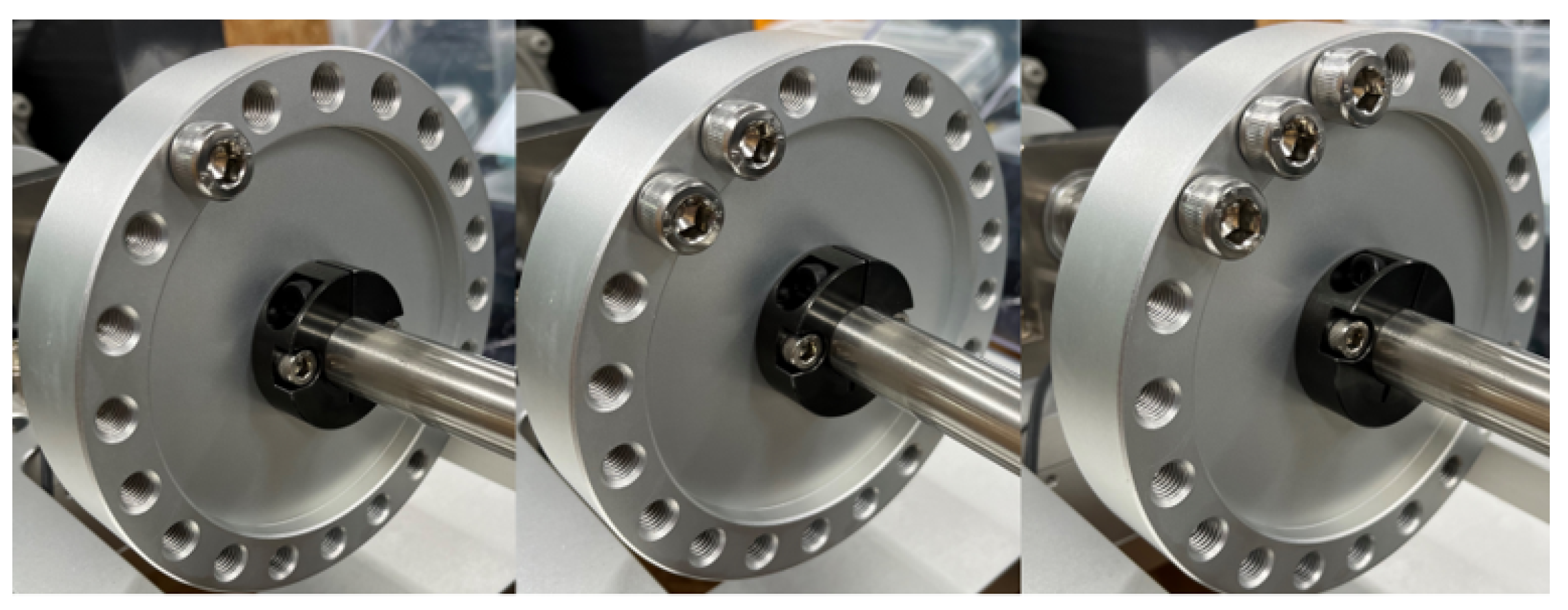
We conducted experiments under three experimental conditions: (1) normal condition, (2) eccentricity fault condition, (3) bearing fault condition. The bearing fault was induced by intentionally drilling holes, and the severity of the fault increased with the number of holes, as shown in Figure 2. The eccentricity fault was induced by adding weights to the rotating body and the fault severity was escalated by increasing the number of weights, as shown in Figure 3.

3. Methodology

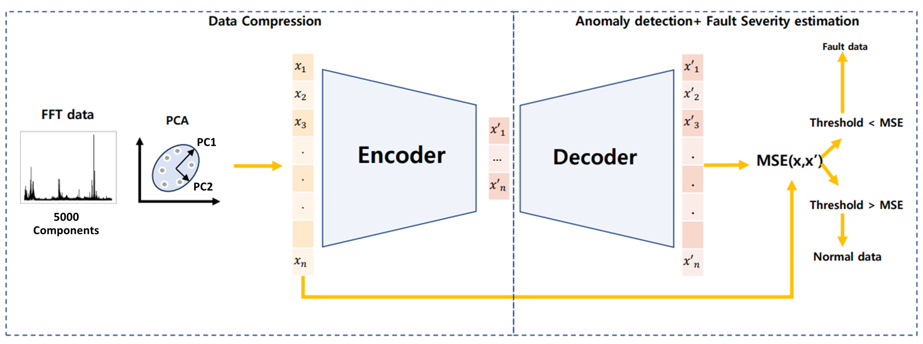
In this section, we will explain the methods that we use in this study. An implementation scheme of our proposed method is shown in Figure 4. The effects of motor faults appear as peaks in the frequency domain. Therefore, we first apply the fast Fourier transform (FFT), which is widely used in vibration analysis, to analyze the frequency domain [46]. We performed the FFT in 0.5 s increments and set the resolution of the FFT to 2 Hz. This resulted in each dataset having 5000 initial components. Given that tens of gigabytes of data are generated per sensor per day, the need for compression is crucial to manage the bandwidth and storage requirements effectively.
We utilize PCA and an AE encoder for data compression. Due to the challenge of collecting fault data in manufacturing environments, we fit PCA using a dataset composed solely of normal data, as well as another dataset containing a mix of 1% anomaly data and 99% normal data. By training the AE exclusively on normal data, it becomes proficient at identifying deviations from typical patterns. To detect faults, we reconstruct the compressed data using the AE decoder and use the mean squared error (MSE) to distinguish between normal and abnormal data. Additionally, we use clustering performance metrics and the t-SNE technique based on the degree of data compression to evaluate the preservation of essential information.

3.1. Principal Component Analysis

PCA is an unsupervised statistical method that can be used for dimensionality reduction and feature extraction [47,48]. PCA aims to transform a high-dimensional dataset into a lower-dimensional space while preserving the most important information. The PCA process involves several steps [49]. First, the data are normalized using Equation (1).
Normalization = X μ σ
where X is the original data, μ is the mean, and σ is the standard deviation Then, the covariance matrix is computed using Equation (2).
Σ = 1 n ( X μ ) T ( X μ )
where n is the number of data, X is the normalized data, and μ is the mean. After that, the principal components are obtained through computing the eigenvectors and eigenvalues of the covariance matrix. Principal components are the directions in which the data vary the most. From the eigenvector matrix, we select the first k columns. The principal components are then used to project the data into a lower-dimensional space using Equation (3),
z = V k T · x
where z is projection, X is the normalized data, V k T is a matrix containing k eigenvectors, and k is the number of eigenvectors that we choose.
We separate the PCA process into two stages: the fitting stage, where we obtain the principal components through eigenvalue decomposition (specifically, V k , as shown in Equation (3)); and the transformation stage, where the original data are projected onto the principal components to obtain a reduced-dimensional representation. In the fitting stage, we applied PCA in two scenarios: one involving only normal data, and the other with a 1% admixture of abnormal data to simulate manufacturing environments. After the PCA fitting process, we calculated the explained variance ratios and compared the results. This comparison allowed us to retain the principal components that explain a substantial portion of the dataset’s variance, achieving effective dimensionality reduction while preserving the most informative aspects of the data.

3.2. Autoencoder

An autoencoder is an artificial neural network that compresses input data into a lower-dimensional latent space, and then, reconstructs it back to its original form. It consists of two components, an encoder and a decoder. The encoder consists of multiple hidden layers that progressively reduce the dimensionality of the input data [50]. The encoder compressed the high-dimensional input data x R n in to latent vectors h R m by a function f θ :
f θ ( h ( i 1 ) ) = s f ( W i × h ( i 1 ) + b i )
where h ( i 1 ) denotes the output of the previous layer. s f is the activation function and we used the rectified linear unit (ReLU) function for the hidden layers and a linear activation function for the latent vectors in this study. W i is the weight matrix for the i t h layer. b i is the bias vector for the i t h layer.
The decoder reconstructs the original input from the latent vectors using a function g θ . At each layer i it applies the function as follows:
g θ ( h ( i 1 ) ) = s g ( W i × h ( i 1 ) + b i )
where s g represents the activation function used in the decoder. In this study, we employed the ReLU function for the hidden layers and a linear activation function for the output layer. W i is the weight matrix specific to the i-th decoder layer. b i is the bias vector specific to the i-th decoder layer.
During training, the AE minimizes the difference between the input data and the reconstructed output [51]. This process is typically achieved by adjusting the neural network parameters to reduce the mean squared error (MSE), which is calculated as follows:
M S E = 1 n i = 1 n ( x i x ^ i ) 2
where n represents the number of data points. x i denotes the original input data. x ^ i represents the corresponding reconstructed output.
Anomaly detection is a powerful application of AEs [35,37,52,53,54]. By training the AE on normal data, it learns to reconstruct the normal data accurately. However, when abnormal data are input during testing, the AE struggles to reconstruct them effectively and it leads to higher reconstruction errors. As a result, data with significant reconstruction errors can be detected as anomalies. In our case, we trained an AE using only compressed normal data for anomaly detection. After training, we used an AE encoder for data compression and an AE decoder for anomaly detection and fault severity estimation. We determined the threshold for anomaly detection by considering the top 5% of the data based on the loss function.

3.3. t-Distributed Stochastic Neighbor Embedding

t-SNE is an unsupervised dimensionality reduction technique aimed at mapping high-dimensional data into a lower-dimensional space while preserving local data structures and inter-point relationships [55]. Therefore, it is appropriate for evaluating compression in latent vectors. t-SNE comprises several key steps, described below [56].
Initially, it applies stochastic neighbor embedding (SNE) to the dataset, transforming high-dimensional Euclidean distances between data points into conditional probabilities, capturing similarities. The similarity between data point x j and data point x i is represented by the conditional probability p j | i , defined in Equation (7):
p j | i = exp | | x i x j | | 2 2 σ i 2 k i exp | | x i x k | | 2 2 σ i 2
In the low-dimensional space, t-SNE uses a student t-distribution with one degree of freedom, as expressed in Equation (8):
q j | i = 1 + | | y i y j | | 2 1 k l 1 + | | y k y l | | 2 1
The t-SNE minimizes the cost function defined in Equation (9), which includes the Kullback–Leibler (KL) divergence to align conditional probability distributions in high- and low-dimensional spaces.
Cost = K L ( P i | | Q i ) = i j p j | i log p j | i q j | i
where P i represents the conditional probability distribution among all data points given a data point x i , and Q i corresponds to the conditional probability distribution over all other mapped points given mapped point y i [57]. The optimization of this cost function is achieved using a gradient descent method.
The ability of an AE to generate a compressed latent space representation demonstrates its effectiveness in capturing essential information from the input data [58]. The t-SNE method can be employed to qualitatively evaluate and visualize the efficiency of data compression [59]. This study utilized the t-SNE method to visualize the distribution of data in the latent space compressed by the AE encoder as a function of the number of latent vectors. This visualization demonstrates the effectiveness of the compressed data in preserving the essential information of the original data.

4. Result

In this section, we discuss the results obtained from applying our methodology to datasets. In manufacturing environments, there can be scenarios where fault data are either unavailable (due to lacking labels) or in limited supply. Therefore, we applied our methodology in two scenarios: one using only normal data during the PCA fitting stage, and another incorporating 1% of anomaly data.

4.1. PCA Fitting with Only Normal Data

We first assumed that there were no fault or labeled fault data. We exclusively applied the PCA fitting stage to the normal data. After completing the PCA fitting process, we obtained the explained variance ratios for different numbers of components, as shown in Table 2. We collected data for 40 min with a sensor with a sampling rate of 20 k, and performed FFT in 0.5 s increments. As a result, 4800 datasets were obtained for each scenario. Accordingly, when we performed PCA, we obtained 4800 components, which is the same number as the maximum number of datasets. To assess the trade-off between preserving information from the original data and achieving data compression, we conducted experiments using various PCA-explained variance ratios of 50%, 60%, and 70%. Through this process, the data were compressed to 1.08%, 2.24%, and 6.64% of the FFT data size, respectively.
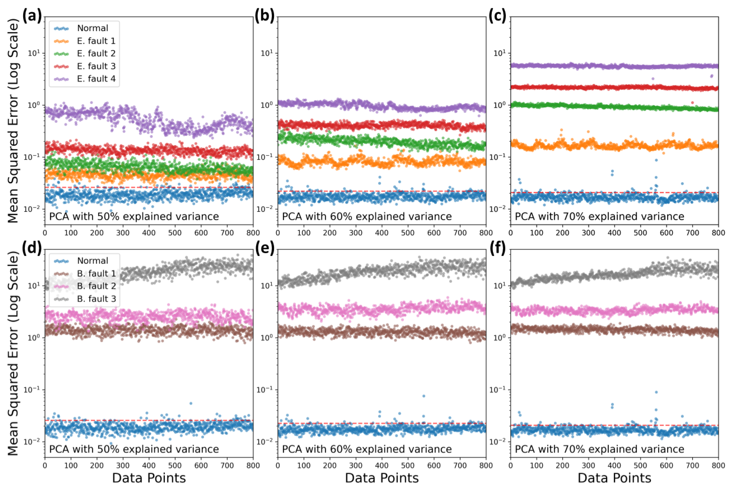
As a tool of anomaly detection and fault severity estimation, we used the AE decoder to analyze both the eccentricity fault datasets and the bearing fault datasets to compute the MSE. The results are depicted in Figure 5, where the number after each label represents the fault severity, i.e., a label number of 1 (E. fault 1, B. fault 1) represents the mildest fault. For anomaly detection, as shown in Figure 5, it is possible to detect anomalies across all explained variance ratios of the dataset, with the MSE increasing as the fault severity increases. The fault detection criterion is the red dashed line, representing the top 5% MSE threshold based on normal data. However, when the explained variance ratio is 50% (Figure 5a,d), it is hard to distinguish between the two lower-severity faults (E. fault 1, 2 and B. fault 1, 2). When the PCA-explained variance ratio is increased to 60% (Figure 5b,e), the MSE difference between the two lower-severity faults becomes more pronounced. In Figure 5c,f, the separation of MSE based on fault severity is clearly visible. This demonstrates the trade-off between the PCA-explained variance ratio and fault severity identification, which is critical for balancing data compression with effective fault detection.
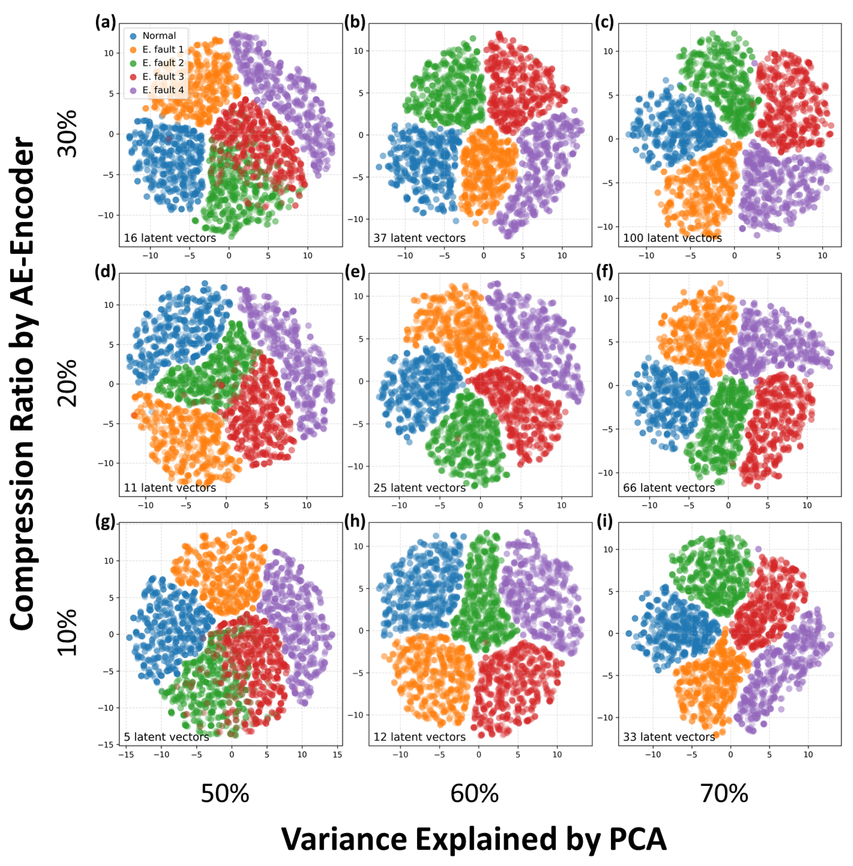
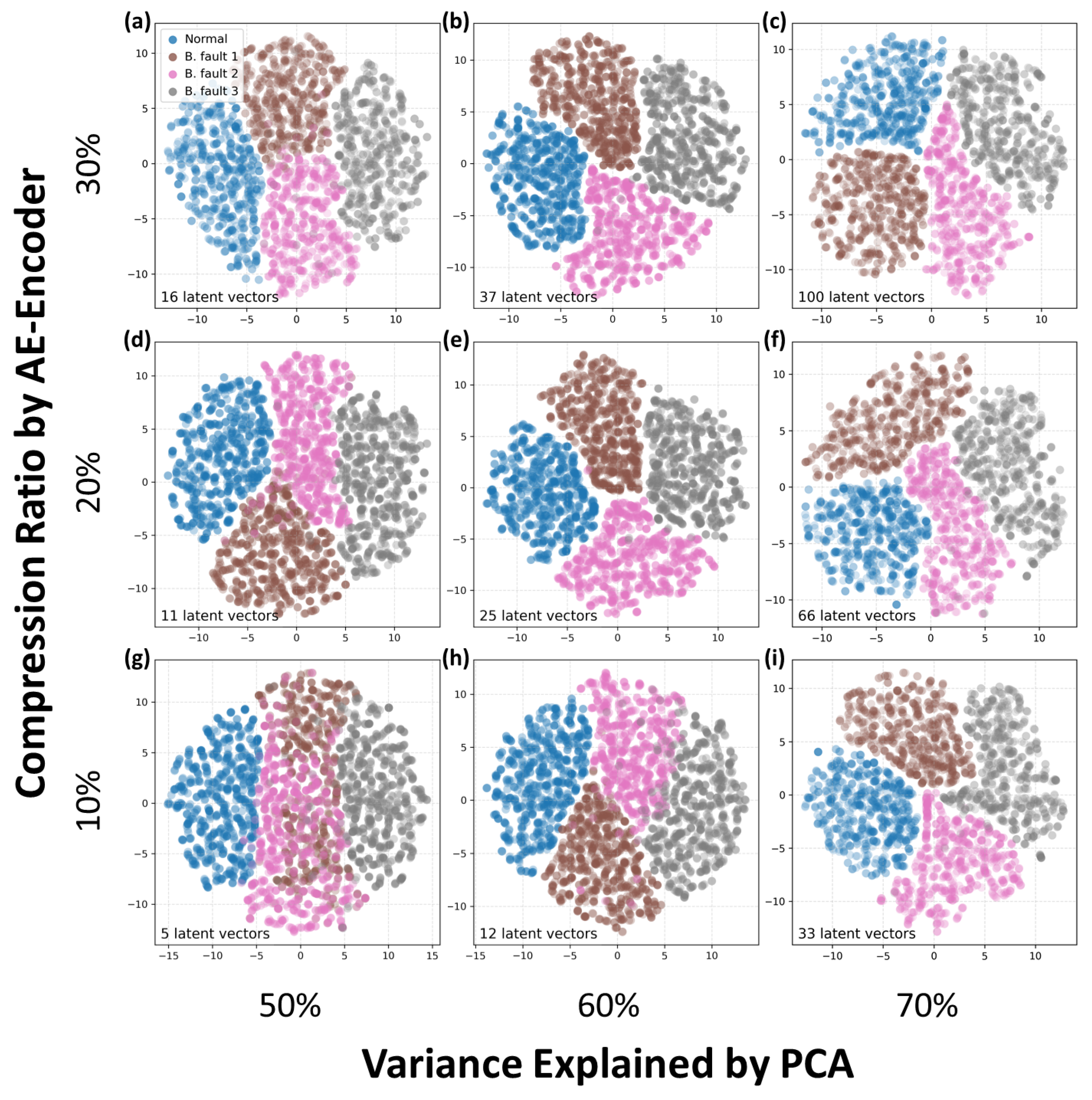
The PCA and AE encoder models, fitted and trained on the normal data, were sequentially applied to generate compressed datasets of eccentricity fault data and bearing fault data to visualize the distribution of the compressed data. This process included the following steps: First, we applied PCA to each dataset and adjusted the number of components to explain 50%, 60%, and 70% of the variance. Specifically, in the PCA model fitted with normal data, 54 components explained 50% of the variance, 124 components explained 60%, and 332 components explained 70% (refer to Table 2). Next, we trained an autoencoder on normal data, where the number of latent vectors was set to 10%, 20%, and 30% of the principal components. For instance, for the PCA with 332 components (70% variance explained), the latent vectors for the autoencoder were 33, 66, and 100, respectively. After training, we applied the autoencoder to compress each dataset (eccentricity fault data combined with normal data and bearing fault data combined with normal data) and visualized the compressed data using t-SNE. The results of these visualizations are presented in Figure 6 and Figure 7. The t-SNE visualization helps reduce uncertain estimates by showing the distribution of the compressed data. This qualitative evaluation demonstrates the trade-offs involved in selecting the appropriate level of compression to ensure data integrity. Following this visual analysis, we use clustering metrics to quantitatively validate the results and ensure the reliability of our methodology.
Figure 8 illustrates the clustering performance results of comparing normal data with two types of fault data using the PCA and AE encoder compression models trained on normal data. Figure 8a shows the results for normal data and eccentricity fault data, while Figure 8b presents the results for normal data and bearing fault data. In this evaluation, data were compressed by adjusting the PCA-variance-explained ratio and the number of latent vectors in the AE encoder, followed by measuring clustering performance. Clustering performance was assessed using three metrics: the Adjusted Rand Index (ARI), normalized mutual information (NMI), and the Fowlkes–Mallows Index (FMI). High clustering scores indicate that despite the data compression, the boundaries between normal and anomalous states, as well as the severity of faults, were clearly distinguished. This implies that the compression techniques maintained the integrity of the data necessary for accurate fault detection and severity classification.
Specifically, when clustering normal data and eccentricity fault data, the most distinct results were observed with a PCA-variance-explained ratio of 60% and AE encoder compression rates of 10% or 20%, corresponding to 25 latent vectors. At this setting, the data compression ratios were reduced to 0.24% and 0.5%, respectively, compared to the original vibration data post-FFT, while still achieving high performance. For normal data and bearing fault data, the clustering performance was relatively lower. However, our approach provides effective compression strategies even for data that are more challenging to cluster. For example, a compression method with an NMI of about 0.67 using only 0.22% of the data can be obtained with a PCA-variance-explained ratio of 50% and an AE encoder compression ratio of 20%. Alternatively, a compression method with an NMI of about 0.76 using 0.66% of the data can be obtained with a PCA-variance-explained ratio of 70% and an AE encoder compression ratio of 10%.

4.2. PCA with 1% Anomaly Data

We also considered the case where a small amount (1%) of fault data are added. During the PCA fitting stage, we utilized a dataset that combined 1% anomaly data with the remaining 99% normal data. For the PCA fitting using eccentricity fault data, we mixed the fault severity levels to reflect actual manufacturing conditions (E. fault 1: 50%, E. fault 2: 33.3%, E. fault 3: 16.7%). For the bearing fault data, there were significant deviations from the normal data, as shown in Figure 5d–f. Mixing data with such large deviations would lead to excessive data compression during the PCA process, resulting in excessive loss of information. Therefore, only the mildest defects (B. fault 1: 100%) were considered in the PCA fitting with the bearing fault data.
The explained variance ratios for each PCA result are presented in Table 3 and Table 4. Despite adding only 1% fault data, a higher explained variance ratio is achieved with fewer principal components compared to using only normal data. The fault data introduce more variability and distinct features, making it easier for PCA to capture significant directions of variance. Fault data often have distinct patterns or anomalies that stand out compared to the homogeneous normal data, allowing PCA to capture these differences more effectively with fewer components.
The performance evaluation results using PCA fitting with 1% fault data are shown in Figure 9. The MSE results (Figure 9a,b,e,f) effectively differentiate fault severity levels. The t-SNE visualization shows that information in the latent space is well preserved. For PCA fitting with eccentricity fault data, 70% explained variance and 30% AE latent vector ratio resulted in 56 latent vectors and a 1.12% compression ratio (Figure 9c,d). For PCA fitting using the bearing fault dataset, only 70 principal components were needed to explain 70% variance, significantly lower than the 188 components for the 1% eccentricity fault dataset and 332 components for the normal dataset. Thus, we used 80% explained variance and 30% AE latent vector count, resulting in 70 latent vectors and a data compression ratio of 1.4% (Figure 9g,h).
The results in Figure 9 also demonstrate the versatility of our method in fault detection and data compression across different fault scenarios. Figure 9b,d show bearing fault data compressed using PCA fitted with 1% eccentricity fault data, while Figure 9e,g show eccentricity fault data compressed using PCA fitted with 1% bearing fault data. These results indicate that our method can effectively be applied to different fault scenarios even with data from only one fault type. This is because PCA captures significant variance directions that indicate fault patterns, which are applicable across different types of faults. By including a small amount of fault data, PCA adapts to capture key features distinguishing normal from faulty conditions. The subsequent AE compression preserves these features in the latent space, ensuring essential fault information is retained. Additionally, selecting an appropriate compression ratio is crucial to maintaining the balance between data reduction and information preservation, ensuring the compressed data are both efficient and effective for fault detection. This adaptability makes our method versatile for real-world manufacturing environments, where comprehensive labeled datasets for all fault types are impractical.

5. Conclusions

This study introduces an innovative approach for PHM of motors in manufacturing environments using edge computing. By addressing the challenges of data volume and processing limitations on edge devices, we developed a data compression method combining PCA and an AE encoder. Our experimental setup involved capturing vibration data under normal, eccentricity fault, and bearing fault conditions using high-resolution sensors. The methodology involved FFT followed by PCA and AE encoder compression. By fitting PCA on normal data and incorporating a minimal amount of fault data, we optimized the compression process. AE models, trained to accurately reconstruct normal data, allowed for effective anomaly detection through mean squared error (MSE) evaluation.
The results demonstrated that our approach could achieve significant data compression ratios while maintaining high accuracy in fault detection and severity estimation. Specifically, PCA combined with AE provided effective compression down to 1.12% of the original data size, enabling real-time analysis on edge devices without significant information loss. The t-SNE visualizations further validated the preservation of essential data characteristics in the compressed space, facilitating clear fault differentiation.
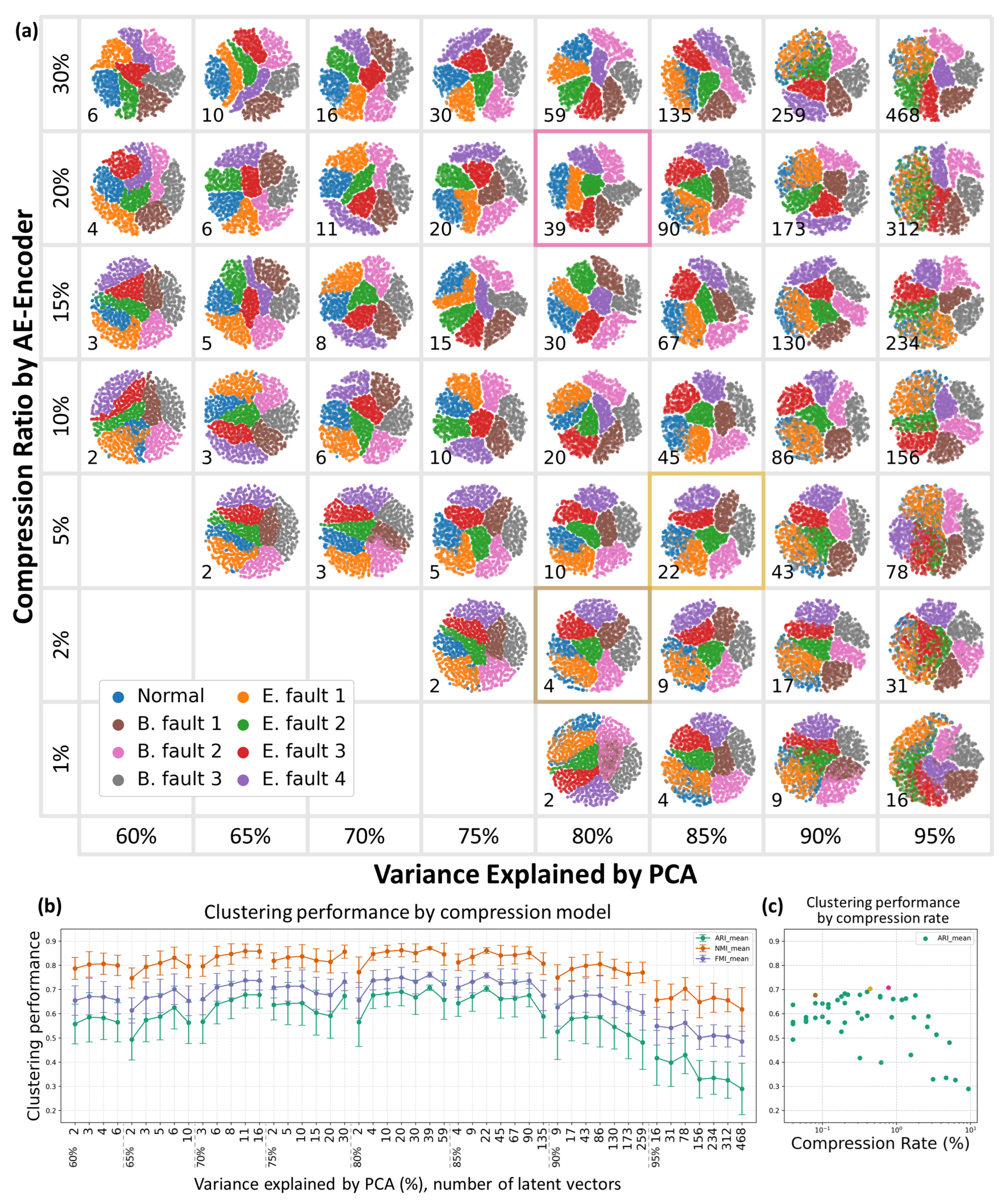
Figure 10 summarizes the clustering performance across different compression ratios and methods, offering both qualitative and quantitative analysis. These results were obtained by using PCA fitted with 0.5% eccentricity fault and 0.5% bearing fault data (E. fault 1: 25%, E. fault 2: 16.7%, E. fault 3: 8.3%, B. fault 1: 50%), demonstrating how well the compression methods preserve the structure of the data across different fault types and severities. Figure 10a shows t-SNE visualizations of data compressed using various PCA-variance-explained ratios and AE compression levels. Figure 10b presents clustering performance metrics, such as ARI, NMI, FMI, for different PCA-variance-explained ratios and the number of AE latent vectors. Figure 10c highlights three representative data points with excellent compression rates and high ARI clustering scores, marked in pink, yellow, and brown. The corresponding t-SNE visualizations in Figure 10a are also highlighted in the same colors. The compression method highlighted in pink uses only 0.78% of the data, in comparison to the FFT data. The yellow and brown methods utilize 0.44% and 0.08%, respectively. These methods demonstrate optimal compression while retaining a reasonable amount of essential information. This demonstrates that our methodology can effectively compress data in a manufacturing environment.
In conclusion, our research provides a viable solution for motor PHM on edge devices, striking a balance between data compression and diagnostic accuracy. By significantly reducing the storage space required and minimizing bandwidth usage for data transmission, our approach enhances the efficiency of data management in manufacturing processes. Additionally, our techniques improve clustering performance and facilitate better fault identification accuracy by leveraging an effective balance in compression degree. Furthermore, our approach includes data structure visualization, which aids in understanding the underlying patterns and relationships within the data. This advancement not only optimizes current manufacturing processes but also lays the groundwork for future innovations in predictive maintenance and operational efficiency.

Author Contributions

Conceptualization, J.H.C. and W.H.C.; methodology, J.H.C. and S.K.J.; validation, H.K.; formal analysis, J.H.C., S.K.J., W.H.C. and S.M.; investigation, S.K.J. and S.M.; resources, J.H.C., W.H.C. and S.M.; data curation, J.H.C. and S.M.; writing—original draft preparation, J.H.C. and S.K.J.; writing—review and editing, S.K.J., W.H.C. and S.M.; visualization, S.K.J., W.H.C. and S.M.; supervision, H.K.; project administration, H.K.; funding acquisition, H.K. All authors have read and agreed to the published version of the manuscript.

Funding

This work was supported by KETI Basic Research Program funded by Korea Electronics Technology Institute (401C3899), Material Innovation Leading Project through the National Research Foundation of Korea (NRF) funded by the Ministry of Science and ICT (2020M3H4A3081879), and Semiconductor Equipment Development Program funded by KoMiKo (41CC4572).

Data Availability Statement

The data that support the findings of this study are available from the corresponding author upon reasonable request.

Conflicts of Interest

The authors declare no conflicts of interest.

References

  1. Lee, J.; Wu, F.; Zhao, W.; Ghaffari, M.; Liao, L.; Siegel, D. Prognostics and Health Management Design for Rotary Machinery Systems—Reviews, Methodology and Applications. Mech. Syst. Signal Process. 2014, 42, 314–334. [Google Scholar] [CrossRef]
  2. Xu, J.; Wang, Y.; Xu, L. PHM-Oriented Integrated Fusion Prognostics for Aircraft Engines Based on Sensor Data. IEEE Sens. J. 2014, 14, 1124–1132. [Google Scholar] [CrossRef]
  3. Guan, F.; Cui, W.W.; Li, L.F.; Wu, J. A Comprehensive Evaluation Method of Sensor Selection for PHM Based on Grey Clustering. Sensors 2020, 20, 1710. [Google Scholar] [CrossRef]
  4. Zhao, J.; Burke, A.F. Electric Vehicle Batteries: Status and Perspectives of Data-Driven Diagnosis and Prognosis. Batteries 2022, 8, 142. [Google Scholar] [CrossRef]
  5. Zhang, W.; Peng, G.; Li, C.; Chen, Y.; Zhang, Z. A New Deep Learning Model for Fault Diagnosis with Good Anti-Noise and Domain Adaptation Ability on Raw Vibration Signals. Sensors 2017, 17, 425. [Google Scholar] [CrossRef]
  6. Wu, S.D.; Wu, P.H.; Wu, C.W.; Ding, J.J.; Wang, C.C. Bearing Fault Diagnosis Based on Multiscale Permutation Entropy and Support Vector Machine. Entropy 2012, 14, 1343–1356. [Google Scholar] [CrossRef]
  7. Xu, G.; Liu, M.; Jiang, Z.; Söffker, D.; Shen, W. Bearing Fault Diagnosis Method Based on Deep Convolutional Neural Network and Random Forest Ensemble Learning. Sensors 2019, 19, 1088. [Google Scholar] [CrossRef]
  8. Meng, H.; Li, Y.F. A Review on Prognostics and Health Management (PHM) Methods of Lithium-Ion Batteries. Renew. Sustain. Energy Rev. 2019, 116, 109405. [Google Scholar] [CrossRef]
  9. Zio, E. Prognostics and Health Management (PHM): Where Are We and Where Do We (Need to) Go in Theory and Practice. Reliab. Eng. Syst. Saf. 2022, 218, 108119. [Google Scholar] [CrossRef]
  10. Cui, L.; Tian, X.; Wei, Q.; Liu, Y. A Self-Attention Based Contrastive Learning Method for Bearing Fault Diagnosis. Expert Syst. Appl. 2024, 238, 121645. [Google Scholar] [CrossRef]
  11. Ding, Y.; Zhuang, J.; Ding, P.; Jia, M. Self-Supervised Pretraining via Contrast Learning for Intelligent Incipient Fault Detection of Bearings. Reliab. Eng. Syst. Saf. 2022, 218, 108126. [Google Scholar] [CrossRef]
  12. Wang, H.; Liu, Z.; Ge, Y.; Peng, D. Self-Supervised Signal Representation Learning for Machinery Fault Diagnosis under Limited Annotation Data. Knowl.-Based Syst. 2022, 239, 107978. [Google Scholar] [CrossRef]
  13. Yu, K.; Ma, H.; Lin, T.R.; Li, X. A Consistency Regularization Based Semi-Supervised Learning Approach for Intelligent Fault Diagnosis of Rolling Bearing. Measurement 2020, 165, 107987. [Google Scholar] [CrossRef]
  14. Chen, C.; Wang, Y.; Ruan, H.; Qin, Y.; Tang, B. A Robust Intelligent Fault Diagnosis Method for Rotating Machinery under Noisy Labels. Meas. Sci. Technol. 2023, 34, 125153. [Google Scholar] [CrossRef]
  15. Miao, J.; Deng, Z.; Deng, C.; Chen, C. Boosting Efficient Attention Assisted Cyclic Adversarial Auto-Encoder for Rotating Component Fault Diagnosis under Low Label Rates. Eng. Appl. Artif. Intell. 2024, 133, 108499. [Google Scholar] [CrossRef]
  16. Zhao, B.; Cheng, C.; Zhao, S.; Peng, Z. Hybrid Semi-Supervised Learning for Rotating Machinery Fault Diagnosis Based on Grouped Pseudo Labeling and Consistency Regularization. IEEE Trans. Instrum. Meas. 2023, 72, 3515812. [Google Scholar] [CrossRef]
  17. Su, H.; Yao, Q.; Xiang, L.; Hu, A. Semi-Supervised Temporal Meta-Learning Framework for Wind Turbine Bearing Fault Diagnosis under Limited Annotation Data. IEEE Trans. Instrum. Meas. 2024, 73, 3512309. [Google Scholar] [CrossRef]
  18. Yan, S.; Shao, H.; Xiao, Y.; Zhou, J.; Xu, Y.; Wan, J. Semi-Supervised Fault Diagnosis of Machinery Using LPS-DGAT under Speed Fluctuation and Extremely Low Labeled Rates. Adv. Eng. Inform. 2022, 53, 101648. [Google Scholar] [CrossRef]
  19. Zhao, X.; Jia, M.; Liu, Z. Semisupervised Deep Sparse Auto-Encoder with Local and Nonlocal Information for Intelligent Fault Diagnosis of Rotating Machinery. IEEE Trans. Instrum. Meas. 2021, 70, 3501413. [Google Scholar] [CrossRef]
  20. Zhang, Y.; Ji, J.; Ren, Z.; Ni, Q.; Gu, F.; Feng, K.; Yu, K.; Ge, J.; Lei, Z.; Liu, Z. Digital Twin-Driven Partial Domain Adaptation Network for Intelligent Fault Diagnosis of Rolling Bearing. Reliab. Eng. Syst. Saf. 2023, 234, 109186. [Google Scholar] [CrossRef]
  21. Li, X.; Li, Y.; Yan, K.; Shao, H.; (Jing) Lin, J. Intelligent Fault Diagnosis of Bevel Gearboxes Using Semi-Supervised Probability Support Matrix Machine and Infrared Imaging. Reliab. Eng. Syst. Saf. 2023, 230, 108921. [Google Scholar] [CrossRef]
  22. Chen, X.; Wang, Z.; Zhang, Z.; Jia, L.; Qin, Y. A Semi-Supervised Approach to Bearing Fault Diagnosis under Variable Conditions towards Imbalanced Unlabeled Data. Sensors 2018, 18, 2097. [Google Scholar] [CrossRef] [PubMed]
  23. Chen, S.; Yang, R.; Zhong, M. Graph-Based Semi-Supervised Random Forest for Rotating Machinery Gearbox Fault Diagnosis. Control Eng. Pract. 2021, 117, 104952. [Google Scholar] [CrossRef]
  24. Pan, H.; Xu, H.; Zheng, J.; Shao, H.; Tong, J. A Semi-Supervised Matrixized Graph Embedding Machine for Roller Bearing Fault Diagnosis under Few-Labeled Samples. IEEE Trans. Ind. Inform. 2024, 20, 854–863. [Google Scholar] [CrossRef]
  25. Maestro-Prieto, J.A.; Ramírez-Sanz, J.M.; Bustillo, A.; Rodriguez-Díez, J.J. Semi-Supervised Diagnosis of Wind-Turbine Gearbox Misalignment and Imbalance Faults. Appl. Intell. 2024, 54, 4525–4544. [Google Scholar] [CrossRef]
  26. Cui, L.; Tian, X.; Shi, X.; Wang, X.; Cui, Y. A Semi-Supervised Fault Diagnosis Method Based on Improved Bidirectional Generative Adversarial Network. Appl. Sci. 2021, 11, 9401. [Google Scholar] [CrossRef]
  27. Li, X.; Zhang, F.L. Classification of Multi-Type Bearing Fault Features Based on Semi-Supervised Generative Adversarial Network (GAN). Meas. Sci. Technol. 2024, 35, 025107. [Google Scholar] [CrossRef]
  28. Zhang, T.; Li, C.; Chen, J.; He, S.; Zhou, Z. Feature-Level Consistency Regularized Semi-supervised Scheme with Data Augmentation for Intelligent Fault Diagnosis under Small Samples. Mech. Syst. Signal Process. 2023, 203, 110747. [Google Scholar] [CrossRef]
  29. Huo, D.; Kang, Y.; Wang, B.; Feng, G.; Zhang, J.; Zhang, H. Gear Fault Diagnosis Method Based on Multi-Sensor Information Fusion and VGG. Entropy 2022, 24, 1618. [Google Scholar] [CrossRef]
  30. Zhu, J.; Jiang, Q.; Shen, Y.; Xu, F.; Zhu, Q. Res-HSA: Residual Hybrid Network with Self-Attention Mechanism for RUL Prediction of Rotating Machinery. Eng. Appl. Artif. Intell. 2023, 124, 106491. [Google Scholar] [CrossRef]
  31. Sun, K.; Liu, D.; Cui, L. Rotating Machinery Fault Diagnosis Based on Optimized Hilbert Curve Images and a Novel Bi-Channel CNN with Attention Mechanism. Meas. Sci. Technol. 2023, 34, 125022. [Google Scholar] [CrossRef]
  32. Wei, Q.; Tian, X.; Cui, L.; Zheng, F.; Liu, L. WSAFormer-DFFN: A Model for Rotating Machinery Fault Diagnosis Using 1D Window-Based Multi-Head Self-Attention and Deep Feature Fusion Network. Eng. Appl. Artif. Intell. 2023, 124, 106633. [Google Scholar] [CrossRef]
  33. Jin, Y.; Yang, J.; Yang, X.; Liu, Z. Cross-Domain Bearing Fault Diagnosis Method Based on SMOTENC and Deep Transfer Learning under Imbalanced Data. Meas. Sci. Technol. 2024, 35, 015121. [Google Scholar] [CrossRef]
  34. Fang, H.; Liu, H.; Wang, X.; Deng, J.; An, J. The Method Based on Clustering for Unknown Failure Diagnosis of Rolling Bearings. IEEE Trans. Instrum. Meas. 2023, 72, 3509508. [Google Scholar] [CrossRef]
  35. Huang, X.; Wen, G.; Dong, S.; Zhou, H.; Lei, Z.; Zhang, Z.; Chen, X. Memory Residual Regression Autoencoder for Bearing Fault Detection. IEEE Trans. Instrum. Meas. 2021, 70, 3515512. [Google Scholar] [CrossRef]
  36. Li, Z.; Xu, P.; Wang, X.B. Online Anomaly Detection and Remaining Useful Life Prediction of Rotating Machinery Based on Cumulative Summation Features. Meas. Control 2023, 56, 615–629. [Google Scholar] [CrossRef]
  37. Xiao, D.; Qin, C.; Yu, H.; Huang, Y.; Liu, C.; Zhang, J. Unsupervised Machine Fault Diagnosis for Noisy Domain Adaptation Using Marginal Denoising Autoencoder Based on Acoustic Signals. Measurement 2021, 176, 109186. [Google Scholar] [CrossRef]
  38. Rezaeianjouybari, B.; Shang, Y. Deep Learning for Prognostics and Health Management: State of the Art, Challenges, and Opportunities. Measurement 2020, 163, 107929. [Google Scholar] [CrossRef]
  39. Shi, W.; Dustdar, S. The Promise of Edge Computing. Computer 2016, 49, 78–81. [Google Scholar] [CrossRef]
  40. Çınar, Z.M.; Abdussalam Nuhu, A.; Zeeshan, Q.; Korhan, O.; Asmael, M.; Safaei, B. Machine Learning in Predictive Maintenance towards Sustainable Smart Manufacturing in Industry 4.0. Sustainability 2020, 12, 8211. [Google Scholar] [CrossRef]
  41. Nain, G.; Pattanaik, K.K.; Sharma, G.K. Towards Edge Computing in Intelligent Manufacturing: Past, Present and Future. J. Manuf. Syst. 2022, 62, 588–611. [Google Scholar] [CrossRef]
  42. Zhou, Q.; Chen, R.; Huang, B.; Liu, C.; Yu, J.; Yu, X. An Automatic Surface Defect Inspection System for Automobiles Using Machine Vision Methods. Sensors 2019, 19, 644. [Google Scholar] [CrossRef]
  43. Kristiani, E.; Wang, L.Y.; Liu, J.C.; Huang, C.K.; Wei, S.J.; Yang, C.T. An Intelligent Thermal Compensation System Using Edge Computing for Machine Tools. Sensors 2024, 24, 2531. [Google Scholar] [CrossRef] [PubMed]
  44. Pedregosa, F.; Varoquaux, G.; Gramfort, A.; Michel, V.; Thirion, B.; Grisel, O.; Blondel, M.; Prettenhofer, P.; Weiss, R.; Dubourg, V.; et al. Scikit-Learn: Machine Learning in Python. J. Mach. Learn. Res. 2011, 12, 2825–2830. [Google Scholar]
  45. Abadi, M.; Agarwal, A.; Barham, P.; Brevdo, E.; Chen, Z.; Citro, C.; Corrado, G.S.; Davis, A.; Dean, J.; Devin, M.; et al. TensorFlow: Large-Scale Machine Learning on Heterogeneous Distributed Systems. arXiv 2016, arXiv:1603.04467. [Google Scholar] [CrossRef]
  46. Wang, Y.; Zheng, L.; Gao, Y.; Li, S. Vibration Signal Extraction Based on FFT and Least Square Method. IEEE Access 2020, 8, 224092–224107. [Google Scholar] [CrossRef]
  47. Wold, S.; Esbensen, K.; Geladi, P. Principal Component Analysis. Chemom. Intell. Lab. Syst. 1987, 2, 37–52. [Google Scholar] [CrossRef]
  48. Dunteman, G.H. Principal Components Analysis; Sage: Newcastle upon Tyne, UK, 1989. [Google Scholar]
  49. Sehgal, S.; Singh, H.; Agarwal, M.; Bhasker, V.; Shantanu. Data Analysis Using Principal Component Analysis. In Proceedings of the 2014 International Conference on Medical Imaging, m-Health and Emerging Communication Systems (MedCom), Greater Noida, India, 7–8 November 2014; pp. 45–48. [Google Scholar] [CrossRef]
  50. Chen, S.; Guo, W. Auto-Encoders in Deep Learning—A Review with New Perspectives. Mathematics 2023, 11, 1777. [Google Scholar] [CrossRef]
  51. Ng, A. Sparse Autoencoder. CS294A Lect. Notes 2011, 72, 1–19. [Google Scholar]
  52. Kraljevski, I.; Duckhorn, F.; Tschöpe, C.; Wolff, M. Machine Learning for Anomaly Assessment in Sensor Networks for NDT in Aerospace. IEEE Sens. J. 2021, 21, 11000–11008. [Google Scholar] [CrossRef]
  53. Wei, Y.; Jang-Jaccard, J.; Xu, W.; Sabrina, F.; Camtepe, S.; Boulic, M. LSTM-Autoencoder-Based Anomaly Detection for Indoor Air Quality Time-Series Data. IEEE Sens. J. 2023, 23, 3787–3800. [Google Scholar] [CrossRef]
  54. Nizam, H.; Zafar, S.; Lv, Z.; Wang, F.; Hu, X. Real-Time Deep Anomaly Detection Framework for Multivariate Time-Series Data in Industrial IoT. IEEE Sens. J. 2022, 22, 22836–22849. [Google Scholar] [CrossRef]
  55. van der Maaten, L.; Hinton, G. Visualizing Data Using T-SNE. J. Mach. Learn. Res. 2008, 9, 2579–2605. [Google Scholar]
  56. Anowar, F.; Sadaoui, S.; Selim, B. Conceptual and Empirical Comparison of Dimensionality Reduction Algorithms (PCA, KPCA, LDA, MDS, SVD, LLE, ISOMAP, LE, ICA, t-SNE). Comput. Sci. Rev. 2021, 40, 100378. [Google Scholar] [CrossRef]
  57. Oliveira, F.H.M.; Machado, A.R.P.; Andrade, A.O. On the Use of T-Distributed Stochastic Neighbor Embedding for Data Visualization and Classification of Individuals with Parkinson’s Disease. Comput. Math. Methods Med. 2018, 2018, 8019232. [Google Scholar] [CrossRef]
  58. Wang, Y.; Yao, H.; Zhao, S. Auto-Encoder Based Dimensionality Reduction. Neurocomputing 2016, 184, 232–242. [Google Scholar] [CrossRef]
  59. Hou, X.; Shen, L.; Sun, K.; Qiu, G. Deep Feature Consistent Variational Autoencoder. In Proceedings of the 2017 IEEE Winter Conference on Applications of Computer Vision (WACV), Santa Rosa, CA, USA, 24–31 March 2017; pp. 1133–1141. [Google Scholar] [CrossRef]
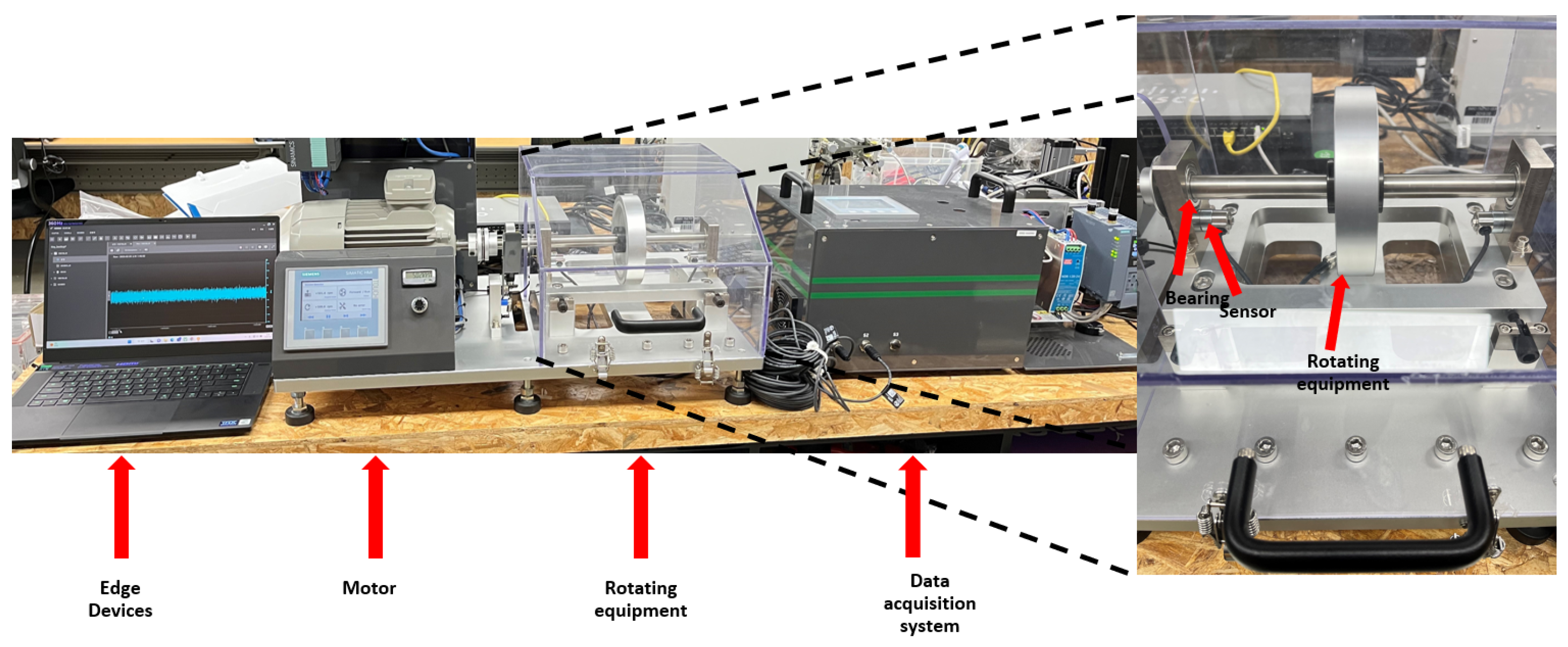
Figure 1. Experimental platform used for data extraction.
Make 06 00069 g001
Figure 2. Detail of bearing fault implementation.
Make 06 00069 g002
Figure 3. Detail of eccentricity fault implementation.
Make 06 00069 g003
Figure 4. An implementation scheme of our proposed method.
Make 06 00069 g004
Figure 5. Calculated MSE of eccentricity and bearing fault datasets using PCA fitted only with normal data. (ac) show MSE results for eccentricity faults (E. fault 1 to E. fault 4) at 50%, 60%, and 70% explained variance. (df) show MSE results for bearing faults (B. fault 1 to B. fault 3) at the same explained variance. Each graph includes a red dashed line indicating the top 5% MSE threshold based on normal data. The legend is consistent across all graphs.
Make 06 00069 g005
Figure 6. t-SNE visualization of normal and eccentricity fault data after compression. (a,d,g) show results where the principal components were selected to explain 50% of the variance. (b,e,h) show PCA with 60% variance explained. (c,f,i) show PCA with 70% variance explained. AE encoder compression rates are 30% in (ac), 20% in (df), and 10% in (gi). The number of latent vectors is indicated in each subplot. The legend colors are consistent across all subplots.
Make 06 00069 g006
Figure 7. t-SNE visualization of normal and bearing fault data after compression. (a,d,g) show results where the principal components were selected to explain 50% of the variance. (b,e,h) show PCA with 60% variance explained. (c,f,i) show PCA with 70% variance explained. AE encoder compression rates are 30% in (ac), 20% in (df), and 10% in (gi). The number of latent vectors is indicated in each subplot. The legend colors are consistent across all subplots.
Make 06 00069 g007
Figure 8. Clustering performance evaluation using PCA and AE encoder compression models fitted and trained with normal data. (a) Normal data and eccentricity fault data. (b) Normal data and bearing fault data. The evaluation was performed by adjusting the PCA-variance-explained ratio and the number of latent vectors in the AE encoder. The legend colors are consistent between (a) and (b).
Make 06 00069 g008
Figure 9. Calculated MSE and t-SNE visualizations of eccentricity and bearing fault datasets. (ad) show results with PCA fitted using 1% eccentricity fault data and 99% normal data. Each graph includes a red dashed line indicating the top 5% MSE threshold based on normal data. (eh) show results with PCA fitted using 1% bearing fault data and 99% normal data.
Make 06 00069 g009
Figure 10. (a) t-SNE visualizations of data compressed using different PCA-variance-explained ratios (60% to 95%) and AE compression levels (1% to 30%). Numbers indicate the number of latent vectors after compression. (b) Clustering performance metrics (ARI, NMI, FMI) for varying PCA-variance-explained ratios and number of AE latent vectors. (c) Clustering performance as a function of the compression rate, with three representative points highlighted in pink, yellow, and brown. The pink method uses 0.78% of the FFT data, yellow uses 0.44%, and brown uses 0.08%. These points show high compression rates and appropriate accuracy, with corresponding t-SNE visualizations highlighted in (a).
Make 06 00069 g010
Table 1. A summary of deep-learning-based fault diagnosis methods for rotating machinery.
ModelReference
Self-Supervised LearningSelf-Attention-Based Signal Transformer[10]
Momentum Contrast Learning (MCL)[11]
1D Convolutional Neural Network (1DCNN)[12]
Semi-Supervised LearningConvolutional Residual Network (CRN)[13]
Deep Neural Networks (DNNs), Two-Component Gaussian Mixture Model (GMM)[14]
Cyclic Adversarial Autoencoder (CAAE), Boosting Efficient Attention (BEA)[15]
Grouped Pseudo-Labeling, Consistency Regularization, Convolutional Neural Network (CNN)[16]
Label Propagation Strategy and Dynamic Graph Attention Network (LPS-DGAT)[17]
Relevant Random Subspace Method for Co-Training (Rel-RASCO), Co-Training by Committee (CoBC)[18]
Semi-Supervised Meta-Learning Framework (SeMeF) with Temporal Convolutional Module[19]
Partial Domain Adaptation Network Driven by Digital Twin[20]
Semi-Supervised Probability Support Matrix Machine (SPSMM)[21]
Visibility Graph Feature (VGF), Graph-Based Semi-Supervised Learning[22]
Random Forest, Graph-Based Semi-Supervised Learning[23]
Semi-Supervised Matrixized Graph Embedding Machine (SMGEM)[24]
Semi-Supervised Deep Sparse Autoencoder[25]
Bidirectional Wasserstein Generative Adversarial Network with Gradient Penalty (BiWGAN-GP)[26]
Semi-Supervised Generative Adversarial Network (GAN)[27]
Generative Adversarial Networks (GAN), Earth Mover’s Distance (EMD), Feature Consistency Regularization (FCR)[28]
Supervised LearningVisual Geometry Group Network (VGG), Convolutional Neural Network (CNN)[29]
Convolutional Neural Network (CNN) and Gated Recurrent Units (GRUs) with Self-Attention Mechanism[30]
Convolutional Neural Network (CNN) with Attention Mechanisms[31]
1D Window-Based Self-Attention and Deep Feature Fusion Network (WSAFormer-DFFN)[32]
Transfer LearningSynthetic Minority Over-sampling Technique Nominal and Continuous (SMOTENC) and Deep Transfer Learning[33]
Transfer Clustering Calculation Center Points (TCCP)[34]
Unsupervised LearningMemory Residual Regression Autoencoder (MRRAE)[35]
Discrete Wavelet Transform (DWT), Regression Analysis[36]
Noisy Domain Adaptive Marginal Stacking Denoising Autoencoder (NDAmSDA)[37]
Table 2. The number of principal components and explained ratio with only normal data.
Number of ComponentsExplained Variance Ratio (%)
112.93
5450.15
8155.00
12460.06
19765.03
33270.00
51475.01
74580.01
104385.00
145190.01
208395.00
4800100
Table 3. The number of principal components and the explained variance ratio obtained by fitting PCA with 1% eccentricity fault data and 99% normal data.
Number of ComponentsExplained Variance Ratio (%)
114.84
2750.02
4455.07
7160.05
11465.05
18870.01
33975.00
56180.01
85885.01
127290.01
192695.00
4800100
Table 4. The number of principal components and the explained variance ratio obtained by fitting PCA with 1% bearing fault data and 99% normal data.
Number of ComponentsExplained Variance Ratio (%)
133.74
750.28
1455.46
2460.21
4165.13
7070.12
12175.03
23480.02
50085.00
91690.01
160695.00
4800100
Disclaimer/Publisher’s Note: The statements, opinions and data contained in all publications are solely those of the individual author(s) and contributor(s) and not of MDPI and/or the editor(s). MDPI and/or the editor(s) disclaim responsibility for any injury to people or property resulting from any ideas, methods, instructions or products referred to in the content.