Real-Time Hybrid Simulation with Deep Learning Computational Substructures: System Validation Using Linear Specimens

Abstract

Hybrid simulation (HS) is an advanced simulation method that couples experimental testing and analytical modeling to better understand structural systems and individual components’ behavior under extreme events such as earthquakes. Conducting HS and real-time HS (RTHS) can be challenging with complex analytical substructures due to the nature of direct integration algorithms when the finite element method is employed. Thus, alternative methods such as machine learning (ML) models could help tackle these difficulties. This study aims to investigate the quality of the RTHS tests when a deep learning algorithm is used as a metamodel to represent the dynamic behavior of a nonlinear analytical substructure. The compact HS laboratory at the University of Nevada, Reno was utilized to conduct exclusive RTHS tests. Simulating a braced frame structure, the RTHS tests combined, for the first time, linear brace model specimens (physical substructure) along with nonlinear ML models for the frame (analytical substructure). Deep long short-term memory (Deep-LSTM) networks were employed and trained to develop the metamodels of the analytical substructure using the Python environment. The training dataset was obtained from pure analytical finite element simulations for the complete structure under earthquake excitation. The RTHS evaluations were first conducted for virtual RTHS tests, where substructuring was sought between the LSTM metamodel and virtual experimental substructure. To validate the proposed RTHS testing methodology and full system, several actual RTHS tests were conducted. The results from ML-based RTHS were evaluated for different ML models and compared against results from conventional RTHS with finite element models. The paper demonstrates the potential of conducting successful experimental RTHS using Deep-LSTM models, which could open the door for unparalleled new opportunities in structural systems design and assessment.

1. Introduction

Hybrid simulation (HS) is a well-established structural testing method that combines experimental components and analytical models simultaneously to evaluate structural elements and overall system behavior under realistic dynamic loading conditions usually from extreme events such as earthquake, wind, etc. Takanashi et al. [1] introduced the first HS in the early 1970s as “on-line testing”, where the non-linear dynamic differential equation of motion was solved with updating the stiffness component of a spring-mass model from the structural experiment at each time step. Since then, there have been numerous studies to expand the range of applications and the applicability of this technique to earthquake loading, then recently, other hazards as well. In general, in HS one or more numerically simulated structural components are replaced by experimental components. In such case, no information on the stiffness of the experimental substructure is needed and a resisting force is fed directly to the hybrid model at each time step to solve the equation and obtain a new input for next time step. This further explains the “online” nature of HS where the input signal to the tested physical specimens in the laboratory are driven by online hybrid model. It is noted that HS is the common term used among the structural and earthquake engineering communities. However, HS can be compared to similar concepts in other disciplines such as the general cyber-physical systems, hardware-in-the-loop systems, etc.

In each time step of the dynamic analysis in HS or real-time HS (RTHS), the differential equation is usually solved with direct integration methods for a coupled experimental/computational model, where the finite element (FE) method has been traditionally used for the computational system. Therefore, one of the main focuses of HS/RTHS studies has been developing numerical integration algorithms specialized on solving the equation of motion for substructured models for efficient and reliable experiment results (e.g., [2,3,4,5]). However, conducting real-time applications could quickly become challenging when the simulated structure has complex computational substructure such as large degrees of freedoms in addition to numerical and/or experimental nonlinearities. It was previously demonstrated by Del Carpio et al. [6] that a careful sensitivity analysis is needed first for large and complex structures to provide accurate and stable simulations. More recently, Bas and Moustafa [7] evaluated currently available direct integration algorithms for RTHS when computational models involve complex nonlinear behaviors. The study concluded that the current integration algorithms might have limitations on conducting RTHS tests when some types of nonlinear behaviors are involved, and experiments become even more sensitive to hardware capabilities. Another important focus of RTHS research studies has been on accurate actuator control. Several efforts have focused on experimental actuator delay compensation and errors amplitude quantification—i.e., results quality and response assessment—due to the nature of combined experimental substructure and the servo-hydraulic actuator [8,9,10,11].

In order to tackle the current challenges and improve RTHS testing advancements, potential alternatives for simulation and control have been explored across various disciplines [12,13,14]. One of those potential alternatives is using machine learning (ML) for computational substructures, which has been introduced by the authors [15] and is further extended through actual testing in this study. ML has recently become a very popular tool to consider in earthquake engineering due to offering advantages such as providing computational efficiency, handling complex datasets, decision-making processes, and treating uncertainties [16]. ML has been widely used in several different earthquake and structural engineering applications, including system identification and damage detection [17,18,19], seismic hazard assessment [20,21], and nonlinear structural response metamodeling [22,23,24,25,26].

In general, ML algorithms can be grouped based on the tasks that are designed to solve, which are namely: classification, regression, and clustering. In this study, the envisioned ML application is regression since the analytical substructure’s dynamic response is aimed to be represented by an ML model. Linear regression (LR) is one of the regression models in ML, which is capable of predicting basic behaviors. In introducing the concept of ML for RTHS, Bas et al. [15] used LR as the metamodel of the computational substructure in the RTHS system for the first time as a simplified model to prove the concept. However, to capture and predict the nonlinear behavior of static and dynamic response of structures, artificial neural networks (ANN) have been widely used during the past decade (e.g., [27]). Mucha [28] used ANNs to represent the analytical substructure in HS to replace the FE models of a bicycle frame and analyzed it under time-varying force. ANNs have been used in several classification and regression problems in the past decade. Yet, ANNs have a simple architecture and one-way output flow (feedforward neural network), which limits their capacity to be used in complicated applications. Therefore, deep learning, which is one of the subgroups of ML, gained increasing popularity for various ML applications.

Deep learning uses stacked layers of neural networks to obtain higher level of features from the input. More advanced deep learning algorithms are recently developed, such as convolutional neural network (CNN) and recurrent neural networks (RNN), which are more suitable for long-range time-varying nonlinear response predictions. Zhang et al. [23] used deep long short-term memory (Deep-LSTM) networks to predict the nonlinear seismic response of structures. To extend the introduced concept of using ML for RTHS and leverage enhanced ML algorithms, the authors conducted some foundational and preliminary work [29] to develop, validate, and verify the communication between Python-based deep-LSTM metamodels, used for RTHS computational substructures, and typical hardware and other RTHS system components. The study successfully integrated Python-based models in RTHS loops and established and validated the communication for RTHS tests with advanced deep learning ML models. However, no actual physical specimens were considered in that foundational study by the authors and there is a need to extend this development further when actual specimens are used. In RTHS, the model is expected to make a prediction based on the online feedback received from the laboratory physical substructure. Thus, there is an obvious need to assess the ML training and resulting models predication under realistic input in RTHS setting.

The overall goal of this study presented herein is to fill the above knowledge gap and build on our previous work [15,29] to conduct actual ML-driven RTHS tests with physical specimens. Thus, our specific objective is to assess the quality of ML training and models for RTHS testing as well as the obtained test results through comparisons with FE-driven RTHS tests. The paper first provides a discussion of the motivation behind this study and how it differentiates and complements previous work by the authors. Then, the paper briefly introduces the HS/RTHS setup and the system configuration where Python is used as computational environment. A one-bay one-story concentrically braced frame (CBF) is used as the case study structure in this paper. The CBF is used to train and evaluate the metamodels under earthquake excitation. For RTHS in this study, the two columns and the beam of the CBF with heavily nonlinear material behavior were considered to be the computational substructure. Meanwhile, the experimental substructure was a physical small-scale steel brace that was kept linear elastic throughout this study to enable accurate validation and assessment comparisons. For the ML modeling, Deep-LSTM networks were used to generate the advanced metamodels that represent the analytical substructures for RTHS. Several online RTHS experiments were conducted without test specimens and then with physical brace test specimens. Moreover, the need and implication of using delay compensator was also investigated for ML-based RTHS tests with and without specimens. For the latter, the adaptive time series compensator (ATS), which was developed by Chae et al. [8], was used for delay compensation. The test results are compared in this paper with virtual RTHS predictions, where metamodel was coupled with analytical experimental substructure, and pure analytical FE solutions to access the quality of the RTHS tests when advanced metamodels are used as computational substructures.

2. Motivation

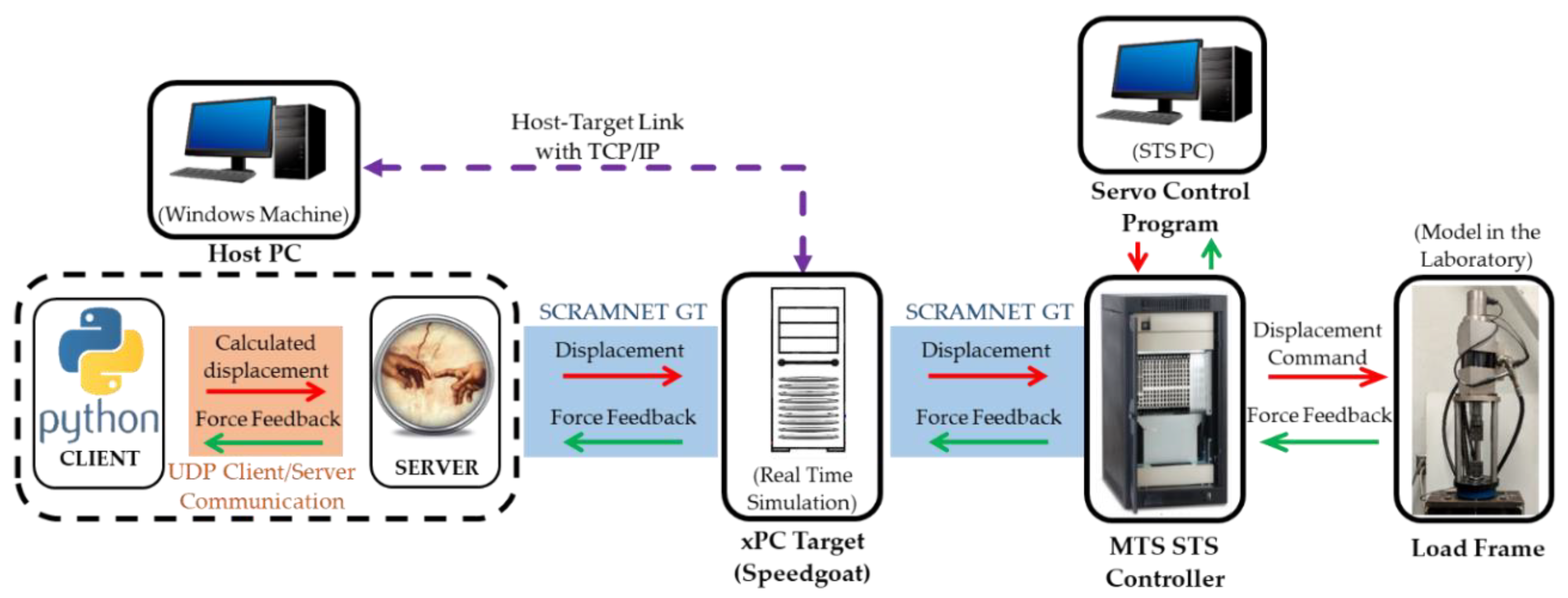
Currently, the use of ML has been rapidly emerging in structural engineering application and is considered a promising alternative approach to obtain surrogate models that can predict structural responses based on available input/output data. Using an ML algorithm representing the FE model for dynamic response prediction gives computationally more efficient results with substantial accuracy. As mentioned earlier, during RTHS, the dynamic differential equation of motion is solved for a coupled numerical-experimental model. Figure 1a illustrates traditional HS where the analytical substructure is modeled using the FE method and coupled with experimental substructure (a brace in the example shown in Figure 1). When experimental substructures are velocity or rate-dependent, HS is conducted in real-time, i.e., RTHS as defined earlier. In order to satisfy real-time requirements at each time step, the equation of motion has to be solved, i.e., numerically integrated, in a limited amount of time that is commonly 10 milliseconds or less. Therefore, once the analytical substructure involves larger degrees of freedoms as well as numerical and/or experimental nonlinear behaviors, conducting real-time testing may not be possible [7]. Thus, using ML metamodel to represent the analytical substructure’s dynamic response in lieu of FE models in RTHS loop could expand RTHS testing capabilities. Such a concept has been proposed by the authors [15,29] and is illustrated in Figure 1b to show how ML models can replace FE models.

Our previous work focused only on communication development for RTHS with Python-based deep learning ML metamodels. Such previous work successfully showed that using metamodels to drive the actuator in RTHS setting is possible and validation was considered using free actuators. In other words, hypothetical linear elastic specimens were used in that study, where an obtained actuator displacement command was multiplied with the constant stiffness value to represent a hypothetical force feedback value at a given time step. Thus, the motivation for this study and how it differentiates from our previous work has three components: (1) consider actual realistic experimental substructures so that the quality of the RTHS test results can be investigated; (2) train two new and different LSTM models for two CBF cases to generalize the results when the dynamic and seismic response vary; (3) conduct and compare results from virtual and actual RTHS tests to assess the deep learning models training quality and prediction performance under ‘idealized’ and actual input from the experimental substructure; and (4) investigate whether using ML-driven RTHS can eliminate the need for using actuator delay compensators (e.g., ATS) that are heavily needed in traditional RTHS tests. Accordingly, the RTHS test results section in this paper provides several scenarios with and without actual experimental specimens and virtual RTHS that are all compared against pure analytical solutions.

3. RTHS Setup

3.1. HS System Components

The recently developed compact HS setup at the Large-Scale Structures Laboratory (LSSL) at the University of Nevada, Reno (UNR) was used for this study [30]. This setup is feasible for many studies including investigating computational challenges in HS/RTHS [7], developing new substructuring concepts [30], developing innovative approaches for computational substructures [29], and for educational demonstrations among other uses.

The FE-based computational substructure of the HS/RTHS can be either modelled in Simulink or OpenSees (an open-source FE simulation software [31]). With the recent developments at UNR [29], Python can be also used as a computational environment to conduct RTHS with ML analytical substructures. The setup is capable of running both slow (pseudo-dynamic) and real-time HS tests. OpenFresco [32] is used as a middleware for the HS tests when analytical substructures are modeled in: (1) specialized FE platforms, e.g., OpenSees that can be run on the Host PC; and (2) Python-based ML models that can also run on the Host PC or even on a high performance computing cluster [29]. Meanwhile, Simulink-based models can be easily compiled and run through a real-time machine such as xPC target. Moreover, OpenFresco has a predictor-corrector algorithm to control different time step ranges between the simulation, integration, and controller. Therefore, the test rate, i.e., constant velocity, pseudo-dynamic, or RTHS, can be controlled through OpenFresco.

The system components at UNR are shown in Figure 2 and more details about such components are explained as follows:

• A small-scale load frame: This is the experimental substructure of the setup. This load frame has a dynamic actuator with 31.14 kN (7 kips) maximum load capacity, ±25.4 mm (± 1 in) stroke, and its peak velocity at no load is 338.84 mm/s (13.34 in/s). The actuator runs with an isolated hydraulic pump with a pumping capacity of 8.71 lt/min (2.3 gpm), and the reservoir capacity of oil volume is 56.78 lt (15 gallons).
• SCRAMNetGT ring: Provides shared memory locations for real-time communication between the various hardware and software hosting components.
• MTS STS controller: Controls the motion of the actuator with 2048 Hz clock speed. It has four channels that allows the system to control up to four actuators simultaneously when needed; however, in the current setup, only one actuator is controlled.
• Real-time high-performance Simulink machine (Speedgoat xPC Target): Provides a high-performance host-target prototyping environment that enables connection of the Simulink and Stateflow models to physical systems. Simulink based analytical models are ran through xPC.
• Host PC (Windows machine): Host PC is where the analytical models (MATLAB, OpenSees, or Python) and the HS middleware OpenFresco are located. The xPC target machine and the Host PC have a TCP/IP connection to set up and initialize the SCRAMNetGT memory locations. Moreover, the Host PC is also assembled with SCRAMNetGT card for real-time applications along with OpenFresco middleware.

3.2. RTHS Configuration

A proper data communication between analytical and experimental substructures is crucial for HS/RTHS experiments. OpenFresco was developed at the University of California, Berkeley to act as an interface software between FE models and the controllers and data acquisition systems in the laboratories to facilitate HS testing [32]. Moreover, it also allows to connect different computational drivers to the HS/RTHS loop. In a recent study by the authors [29], a novel communication scheme was developed to connect the Python environment to the HS/RTHS loop using OpenFresco. This section briefly explains the recent developments when Python-based ML models are used as computational substructures. It should be noted that there are two possible Python environment locations to use within the RTHS loop: Local PC, i.e., Host PC, or cluster such as high-performance computers, supercomputers, etc. In this section, only communication with the Local PC is explained. However, interested readers are referred to Bas and Moustafa [29] for more detailed information about the communication with clusters.

Figure 3 schematically shows the communication loop and details when Python-based metamodel substructures are located in Local PC (Host PC) for RTHS. As mentioned earlier, the Host PC is where the xPC connections are made to set up SCRAMNetGT memory locations and initialize the simulations. The architecture of OpenFresco communication is called the “client&middle-tier server”. In this architecture, OpenFresco is the middle-tier server, where Python is the client. OpenFresco and Python communication is established through UDP/TCP channel. Since the OpenFresco side is the server of the UDP/TCP connection, the channel is opened at the OpenFresco side, and the simulation application site is set. On the Python side, the ‘socket’ module is used for connection set up with either TCP or UDP protocols. Therefore, the client, i.e., Python, connects the open connection provided by the server. The UDP protocol is used in this study for the Python and OpenFresco connection. On the other hand, the OpenFresco also connects to the experimental site. In this study, the local experimental site was used. Furthermore, the interface with the laboratory hardware was defined with the experimental control, where the xPC target transfers data that is obtained from the Host PC to/from the controller. In this HS setup, the xPC target and the Host PC connection can be either provided with TCP/IP or SCRAMNetGT connection. The SCRAMNetGT secures more stable and faster data transfer over TCP/IP connection. Therefore, the SCRAMNetGT connection was used as the experimental control for this study.

Briefly, the data transfer concept of the RTHS setting is explained as follows. The analytical substructure (metamodel) runs from Python, and the input displacements are calculated at each time step to be sent to the experimental substructure as displacement command. The force from the experimental substructure is measured from the specimen and fed back into the metamodel. The time step synchronization between the controller, integration, and simulation is satisfied through the predictor–corrector algorithm that is defined in OpenFresco. For the computational substructures with metamodels, the integration time step becomes the prediction time step since there is no integration processed with metamodels. In this study, the prediction time step and the simulation time step were set to be 0.02 s, which was also the same used for the ML training time step as explained later.

4. Modeling Assumptions

Deep LSTM networks were considered in this study to develop the metamodels that are in turn used to represent nonlinear analytical or computational substructures for RTHS. The training dataset was obtained from pure analytical responses of the overall structure. This section first introduces the FE model that was used to generate the training dataset. The section also explains the methodology for the deep learning algorithm and hyperparameter calibrations of the metamodels.

4.1. Model Parameters and Training Dataset

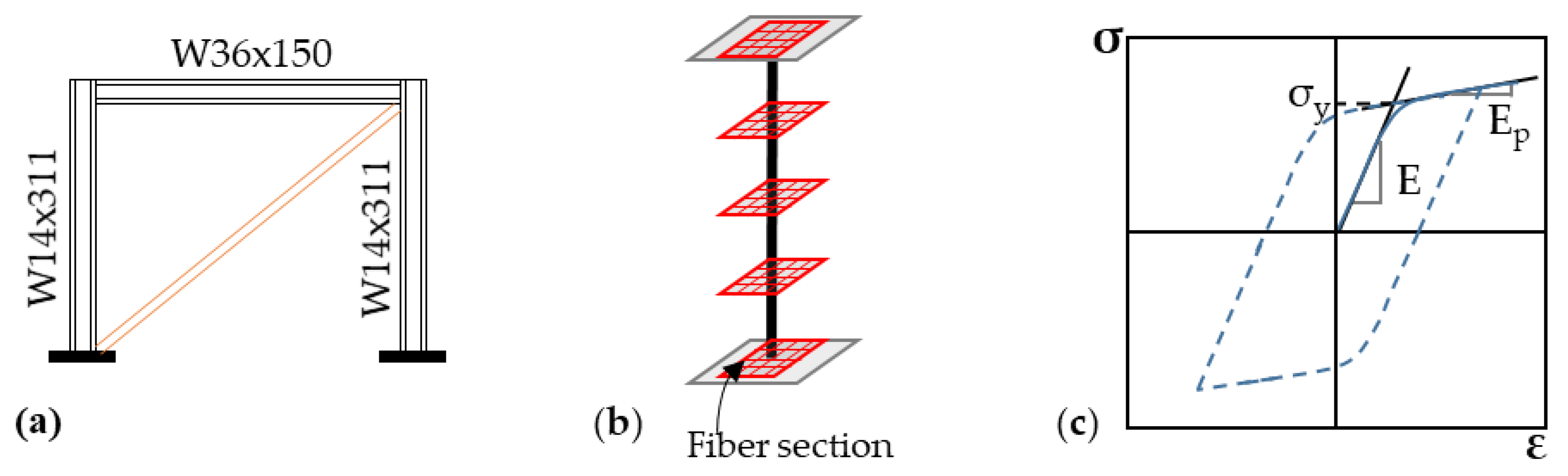
The features of the structure used in this study, and in turn, the parameters for the FE model used in this study is introduced here. This model is what was used in the training of the LSTM metamodel and identifying the training dataset as explained in this section. As mentioned before, a one-bay one-story CBF was selected to be the case study structure, and was trained under earthquake excitation to be used in the RTHS experiments. CBFs are suitable for substructuring where typically braces experience complex behavior that is hard to model numerically, such as buckling, and is more suitable to be experimentally tested. However, for this study the experimental braces were tested only in the linear elastic range for other purposes such as assessment and verification. Concurrently, the columns and beams of CBFs are easier to model with high accuracy and in turn, are suitable for analytical substructuring in HS setting. In the HS setup presented in Section 3.1, a small-scale brace—i.e., the experimental substructure—was combined with an analytical substructure for a prototype steel frame at the full scale. In the present study, the analytical substructure was modeled with material nonlinearity and was represented accordingly in the sought LSTM models. Two RTHS cases were utilized: without specimen and with the specimen. For the cases without a specimen, no physical brace was used so the actuator was free to move. However, the actuator’s displacement was multiplied by a constant stiffness to generate a hypothetical force feedback that represent a linear elastic test specimen. For the cases with the actual physical specimen, the specimen was tested only within in the linear elastic range. That is to establish a case that could be compared against full pure analytical models, which is desired for proper assessment of the performance of RTHS with deep learning models.

The pure analytical model of the CBF was modeled in OpenSees [31]. The columns (W14 × 311) and beam (W36 × 150) elements were modeled with fiber sections along with the distributed plasticity as illustrated in Figure 4. The nonlinear steel material model was defined using uniaxial Giuffré–Menegotto–Pinto material with isotropic strain hardening [33], which is known as Steel 02 in OpenSees and illustrated in Figure 4 as well. The yield stress of the material was selected to be 250 MPa, and the elastic modulus 200 GPa. As mentioned earlier, the experimental substructure is considered to remain linear elastic for the purpose of this study. In order to get the brace characteristics, two specimens were tested under increasing scale cyclic loading (Figure 5). The axial stiffness of the brace in the linear elastic phase was obtained as 46.76 kN/mm. The geometric or length scale (S_L) was 25 for the small-scale brace, which represents a prototype brace with 1169 kN/mm axial stiffness in prototype scale. Again, the experimental substructure was selected to remain linear elastic for both types of RTHS, i.e., with and without specimen cases, to make a valid comparison for quality assessment.

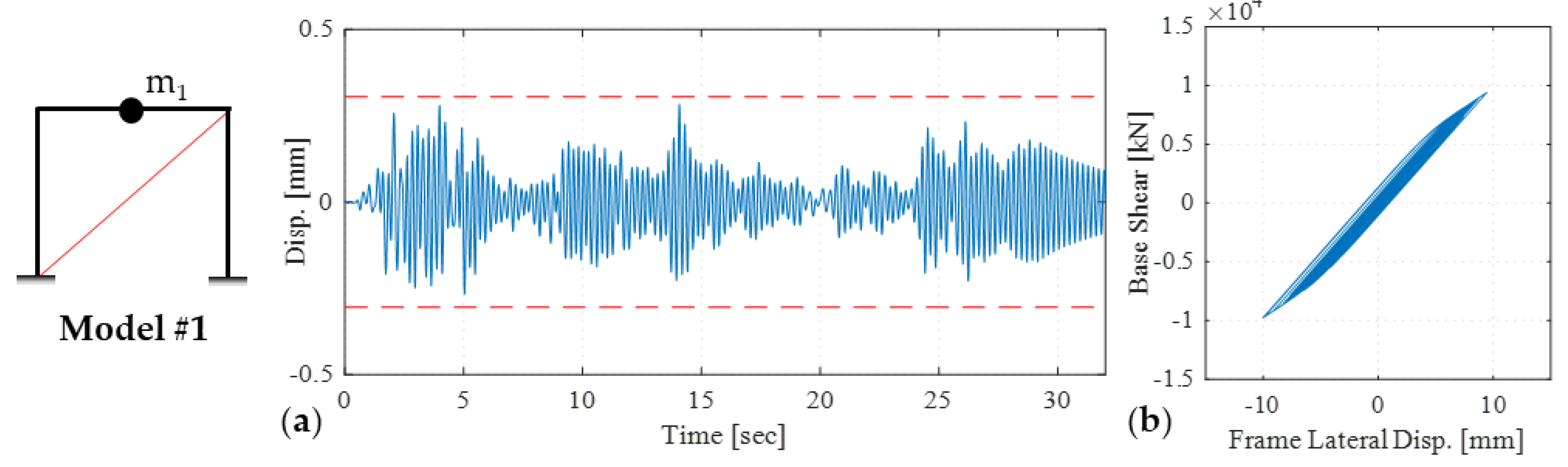
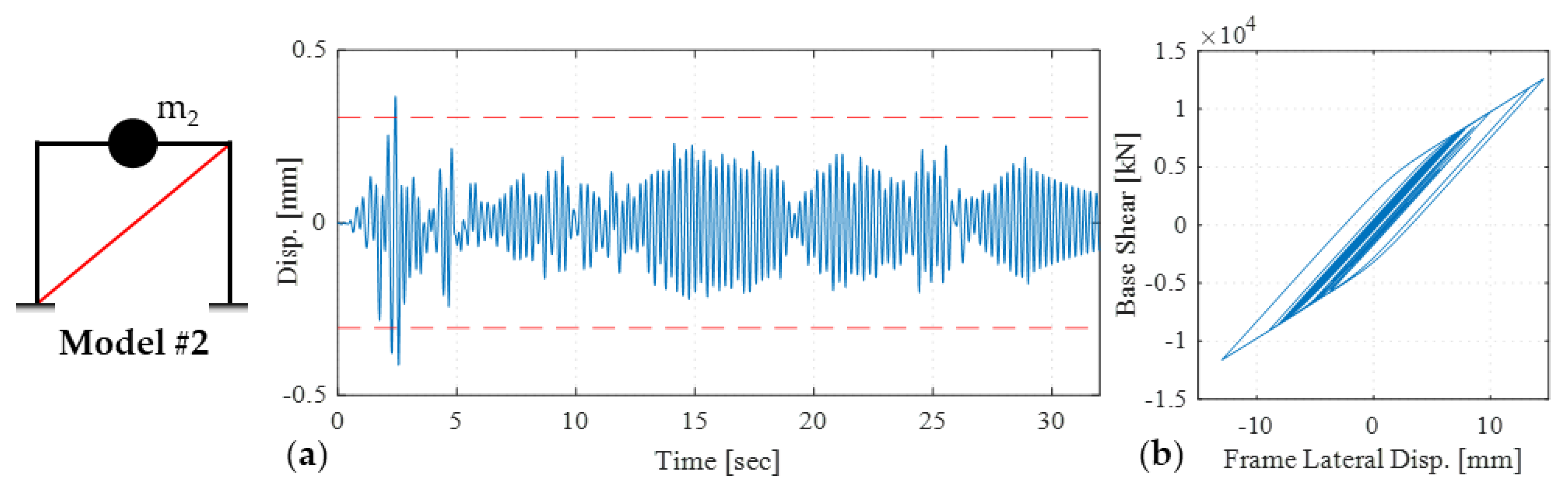
In this study, to guarantee that the brace remained in linear elastic range, two different analytical models were considered with different mass assignment: 1.40 kN-s²/mm (i.e., m₁) and 1.75 kN-s²/mm (i.e., m₂). The frame with lighter mass, designated as Model 1, had a natural vibration period of 0.22 s, while the other frame, i.e., Model 2, had a 0.25 s period. The inherent damping of the structure was modeled using 2% mass proportional damping.

The nonlinear time history analysis of the pure analytical CBFs was conducted under the popular ground motion from 1940 El Centro earthquake. The implicit Newmark method (average acceleration) was selected as the integration algorithm with 0.001 s time steps. The duration of the earthquake record is 31.2 s, but the analysis was carried out for 32 s. For the purpose of training of the metamodels, the dataset was resampled at 0.02 s time step, which led to 1600 data points for each response. The brace displacement time histories for Model 1 and Model 2 are given in Figure 6 and Figure 7, respectively, where the yield displacement is marked with red dashed lines. It can be seen that for Model 1, the brace behavior remains linear elastic, i.e., does not exceed yield displacement, when response is obtained from the pure analytical model. Moreover, the global frame force–displacement relationship was also obtained for both models and also shown in Figure 6 and Figure 7. From the global frame response, it can be seen that Model 2 experienced slightly larger hysteretic loops—i.e., higher nonlinearities—and the brace just slightly exceeded the yield displacement, when compared to Model 1.

The training dataset inputs for the deep LSTM network were selected to be the earthquake ground motion acceleration and the brace force time history, while the output (prediction) of the metamodel was the displacement of the brace, i.e., input for the experimental substructure. During RTHS testing, the force of the brace is dependent on the brace displacement due to the nature of the closed-loop system. This dependency generates a high-level uncertainty in the metamodel, which can lead to unstable predictions. Moreover, the load frame itself has its own uncertainty and other sources of errors due to the nature of the servo hydraulic system. Thus, the training surface was expanded by introducing a systematic bias to the brace force time history as explained in next section. The training dataset was expended with six more cases using offsets of ±5%, ±10%, and ±15% on the brace force. Accordingly, the input had 11,200 data points that covered seven cases of the force input and bias. However, it is noted that the same ground motion data was repeated seven times for the seven cases of force and bias. This is because the bias is not meant to represent a different test or ground motion intensity, but rather an embedded systematic error for the given intended ground motion input.

4.2. Model Parameters and Training Dataset

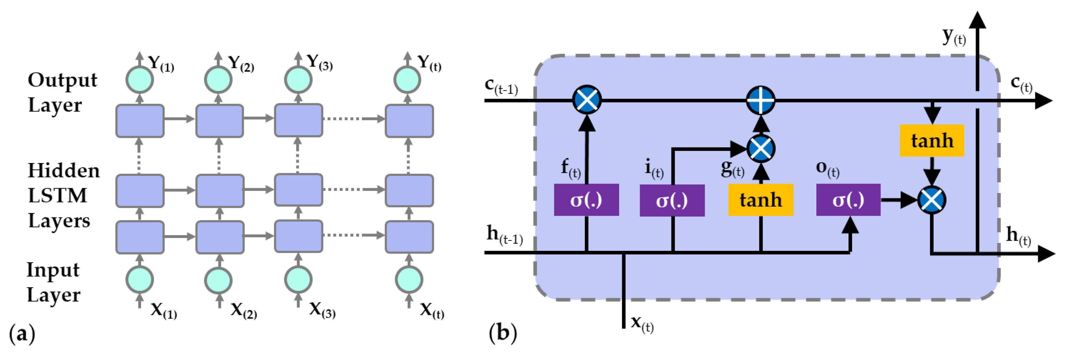
As previously mentioned, deep LSTM networks were selected and used here in this study to model the analytical substructure of the RTHS system. It is noted that other models were checked such as recurrent neural network (RNN), which is one of the most popular ML algorithms for predicting time series. The advantage of RNN over other ML algorithms is that it has a backward connection point, and thus, the layers can get an additional input that is the model output from the previous time step. However, RNN models have two main drawbacks: (i) having a limited short-term memory, and (ii) having unstable gradients [34]. Thus, models like RNN were not found to be promising for the application in hand, and the LSTM model was selected and used instead, LSTM cells are developed to converge faster and detect the long-term dependencies of the datasets as discussed next.

An LSTM network and a cell architecture are represented in Figure 8. In every time step, the LSTM cell receives two additional inputs other than (x(t)), which are to represent short-term states (h(t-1)) and long-term states (c(t-1)). The previous time step output vector (h(t-1)) and current time step inputs (x(t)) are fed into four different fully connected layers. In a regular RNN cell, there is only g(t) layer, which is the weighted sum of the inputs with an activation function of tanh. The other three gate controllers are the ones that help to control memory information for longer sequences and use the logistic function as an activation function (0 or 1). The long-term state’s unnecessary parts are deleted at the forget gate (output of f(t)). The input gate controls which parts of g(t) should be added in the long-term state. Moreover, the parts of the long-term state should be the output to both h(t), and the output gate (o(t)) manages y(t). The equations for the LSTM cell computations are briefly given in Equations (1)–(6). In the equations, W_xi, W_xf, W_xo, W_xg, are the weighted matrices for the input vector and W_hi, W_hf, W_ho, W_hg are the weighted matrices of the previous short-term state vector h(t-1) for each layer. Moreover, every layer has the bias term which are $b_{\mathrm{i}}$, $b_{\mathrm{f}}$, $b_{\mathrm{o}}$, and $b_{\mathrm{g}}$.

$$i_{\left(t\right)}=\sigma \left(W_{xi}{}^T{x}_{\left(t\right)}+W_{hi}{}^T{h}_{\left(t-1\right)}+b_i\right)$$

(1)

$$f_{\left(t\right)}=\sigma \left(W_{xf}{}^T{x}_{\left(t\right)}+W_{hf}{}^T{h}_{\left(t-1\right)}+b_f\right)$$

(2)

$$o_{\left(t\right)}=\sigma \left(W_{xo}{}^T{x}_{\left(t\right)}+W_{ho}{}^T{h}_{\left(t-1\right)}+b_o\right)$$

(3)

$$g_{\left(t\right)}=\tanh \left(W_{xg}{}^T{x}_{\left(t\right)}+W_{hg}{}^T{h}_{\left(t-1\right)}+b_g\right)$$

(4)

$$c_{\left(t\right)}=f_{\left(t\right)}\otimes c_{\left(t-1\right)}+i_{\left(t\right)}\otimes g_{\left(t\right)}$$

(5)

$$y_{\left(t\right)}=h_{\left(t\right)}=o_{\left(t\right)}\otimes tanh\left(c_{\left(t\right)}\right)$$

(6)

The training of the deep LSTM model was done in Python environment using Tensorflow 2.0 [35]. The LSTM model input sequences require three-dimension (3D) arrays, which are batch size (number of samples of the dataset), lookback (previous time steps), and size of the input dimension (number of the features) [34]. The hyperparameters of the LSTM network were tuned by feeding the inputs and the output datasets to the model. The optimizer of the training was selected to be an Adam (Adaptive Moment Estimator) optimizer with a learning rate of 0.001 [36]. The number of epochs was set to be 10³. Moreover, the model was trained to minimize the cost function of mean squared error (MSE). Based on a previous study by the authors [29], two deep learning models were trained to be used with 10 and 15 lookbacks. Each model had an input layer, four LSTM layers with 30 units/layer, and one dense layer, which is a fully connection layer that outputs the prediction.

5. Online RTHS Tests

In this section, the deep LSTM network models which were trained for the two CBF models, i.e., Model #1 and Model #2, with lookbacks 15 and 20, were used and evaluated for RTHS tests. Hereafter, the models with 15 lookbacks are referred to as Model 1a and Model 2a, and the ones with 20 lookbacks are referred to as Model 1b and Model 2b, respectively. In order to investigate the quality of the ML models within the HS loop, two sets of RTHS tests were considered. In the first set, the tests were conducted without a real specimen, but a hypothetical specimen was represented by multiplying the actual actuator displacement by a constant stiffness value to obtain the force feedback. The second set used actual specimens but as mentioned before, the selected ground motion and frame characteristics were supposed to keep the brace within the linear elastic range. The use of a delay compensator was also evaluated during the tests. Thus, all sets of RTHS tests were conducted twice with and without using the ATS compensator and designated in figures as wATS or woATS, respectively. One last variable that was considered in this assessment was related to the force input through the lookback dimension where either the first or last dimension was updated with the actuator force feedback. Therefore, a total of 32 different RTHS tests were conducted and selected test results are presented and discussed here. The experimental substructure response as obtained from the RTHS tests is represented with both force–displacement relationship as well as force and displacement time histories. The error calculations for all 32 tests are also discussed. Moreover, to make a careful evaluation of the deep learning models within the experimental setup, error calculations for virtual RTHS tests are also presented. The virtual RTHS tests are meant to reveal how the LSTM models predictions can vary when using RTHS feedback from an ‘idealized’ analytical FE model versus experimental setup, i.e., analytically and experimentally simulated linear elastic brace behavior. The variation is such cases would be attributed to how the experimental feedback can be contaminated due to laboratory, hardware, and experimental errors, which makes the equivalent feedback from an FE analytical simulation ‘idealized’.

5.1. Experimental Substructure Response: Force–Displacement Relationship

Firstly, the experimental substructure responses for each model and each RTHS test type, i.e., with specimen and without specimen, are presented. Only selected test cases are presented here for the discussion, which are the tests that used the first term of the force input through the lookback dimension for the update. As explained in the training dataset, a systematic bias was introduced to the force input to increase the training domain in an attempt to represent and capture potential force feedback uncertainties because of force–displacement dependencies and initial load frame feedback.

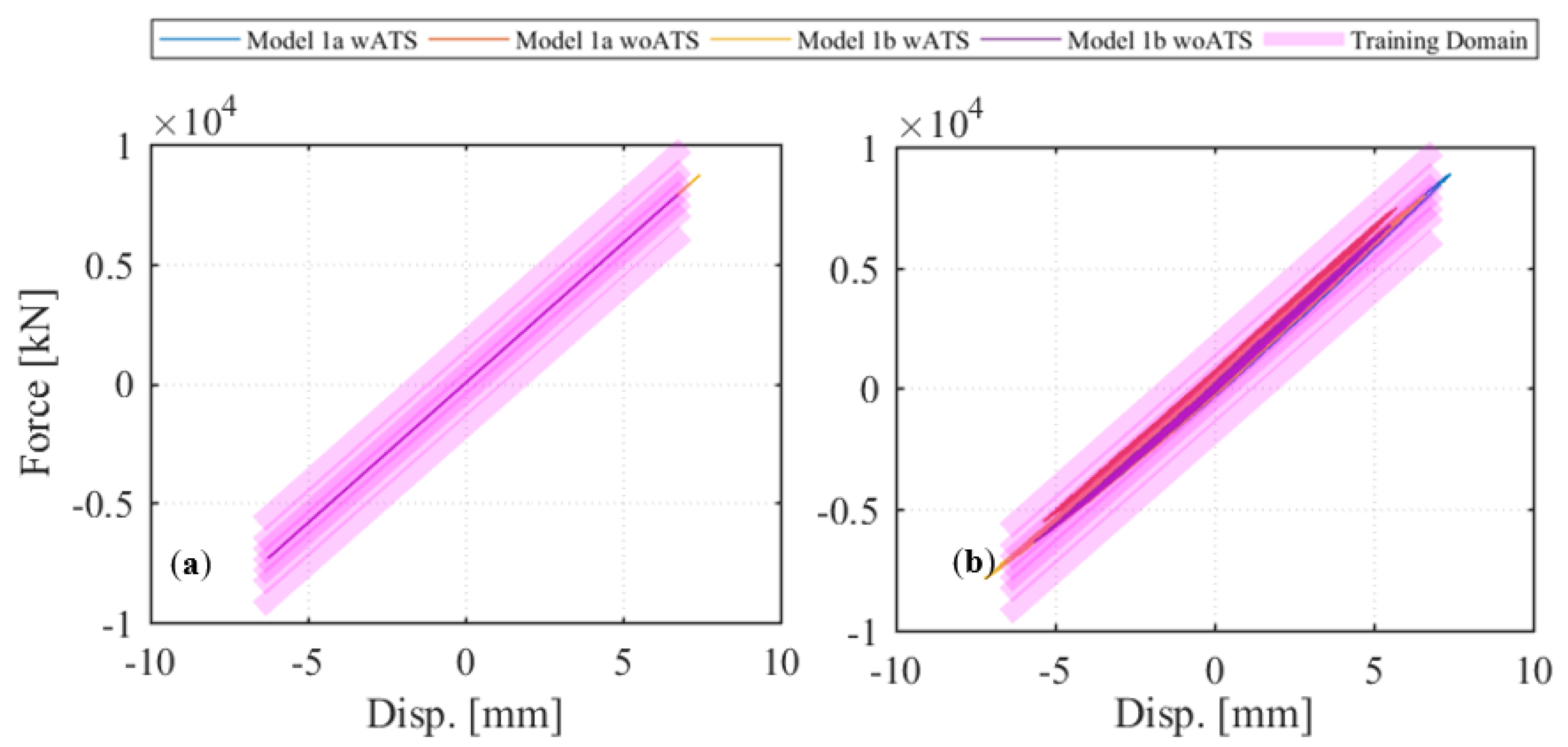
Figure 9 shows the equivalent brace axial force–displacement relationship at the prototype CBF full-scale from the two RTHS tests for Model 1 with and without specimen. It is noted that the applied actuator displacement commands and retrieved force feedback from the experimental specimen are scaled down by S_L = 25 and up by S_L² = 625, respectively, to adjust for the varying geometric scale between physical substructure (brace) and analytical substructure (CBF). It can be seen from the figure that the actual observed actuator response in the case of no specimen—i.e., hypothetical brace case—falls within the training domain as desired. The test results when the real specimen was used (Figure 9b) also confirms that the actual brace remained linear elastic through the RTHS tests as desired. Moreover, the brace force–displacement relationship also falls within the training domain, which confirms that reliable test results can be obtained when deep learning models are considered for computational substructures. The figures also suggest that expanding the training domain in the way proposed and adopted by the authors, i.e., introduced systematic bias, worked well. No stability problems occurred, and both tests with and without actual specimens were successfully conducted.

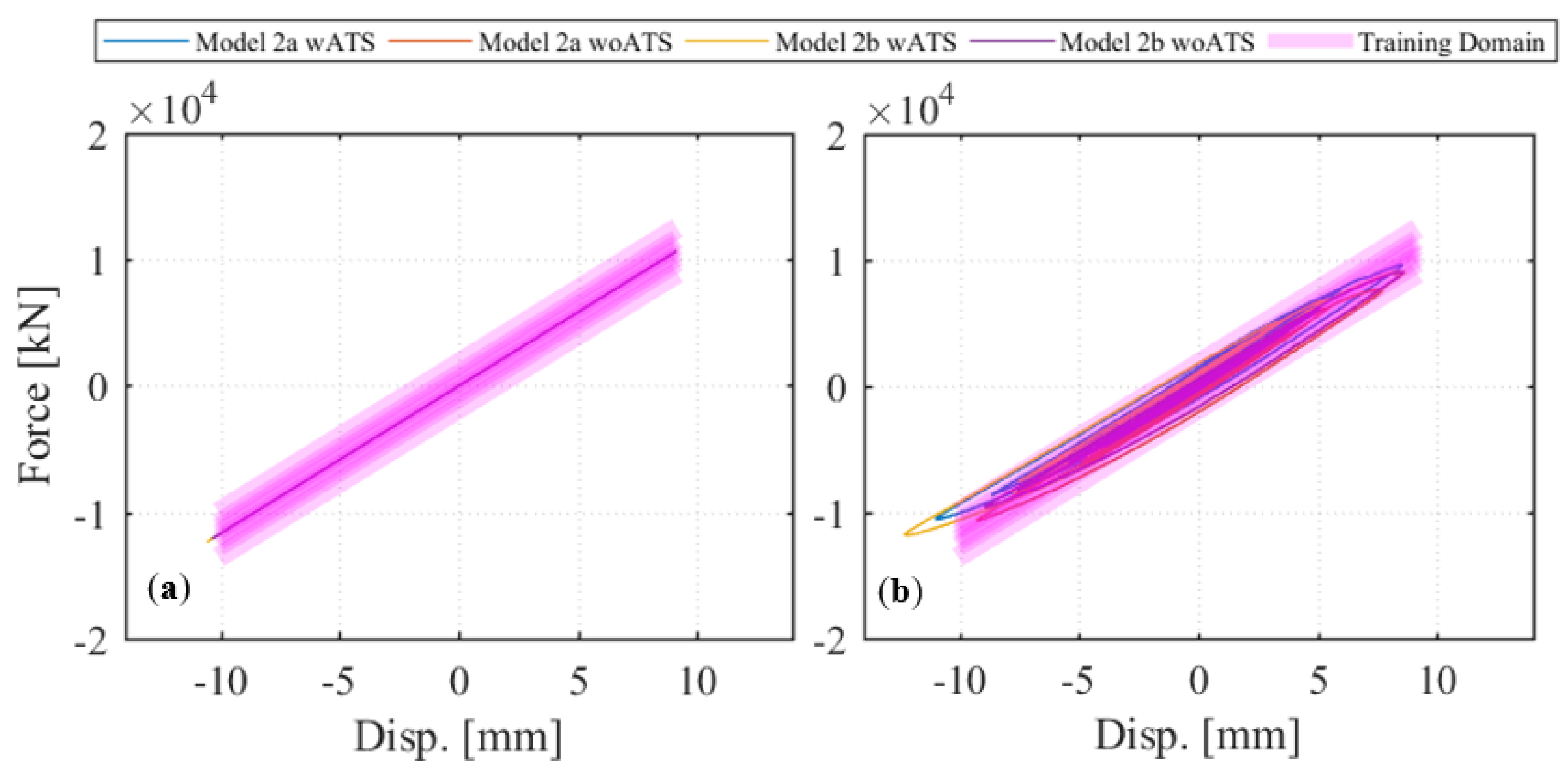
The RTHS test results for Model 2a and Model 2b, which were expected to slightly get into the nonlinear range when compared to Model 1 counterparts, are presented. The equivalent brace axial force–displacement relationship at the prototype full-scale is shown in Figure 10. The values in Figure 10 present up-scaled forces and displacements by similitude scale of 625 and 25, respectively, with respect to actual tested physical specimen scale. For the models where no actual specimen was used, the tests performed well (see Figure 10a). As shown above in the training phase, it was observed that the brace displacement in Model 2 slightly exceeded the yield displacement. The implications of that showed itself in case of RTHS tests with the specimen. It can be seen from Figure 10b that the actual specimen showed some minor hysteretic loops, which is not considered severe nonlinearity. Moreover, the specimen was used repeatedly in other tests without showing any plastic behavior, which confirms that the specimen in general remained linear elastic. The most important observation from Figure 10 is that the devised training domain contained all the minor hysteretic loops, and in turn, ensured a stable test through the end. Again, this is another confirmation that expanding the training domain worked well and led to successful execution of RTHS tests with no stability issues. It is also noted that both Figure 9 and Figure 10 compare cases with and without using the ATS. It is observed from the figures that using the ATS delay compensator did not have any significant effect on test results for both models and each ML-driven RTHS test type.

5.2. Experimental Substructure Response: Force and Displacement Time Histories

In this part, the displacement and force time histories for the experimental substructure responses are shown and compared with the training force input and output displacement datasets. For this evaluation, selected test results from what we consider ‘good’ and ‘bad’ tests are shown and discussed. In Section 5.1, it is shown that ML-driven RTHS with specimens can be successfully executed without stability issues. However, no every successfully completed test is a valid test as there could be large errors in the interpreted response. In this section, we try to take a deeper look at the quality of the test results. This is possible through comparisons with virtual RTHS scenarios where the deep learning models are expected to provide better predications with no experimental errors involved. Moreover, comparisons are also provided against pure FE analytical solutions that represent exact solutions in the case of the linear elastic brace considered for this study.

5.2.1. Selected Results from ‘Good’ RTHS Tests

In this section, RTHS test results from good tests are presented. Model 1b RTHS test results are selected when delay compensator was used. For the force input, the first lookback dimension was updated with the force feedback from the experimental substructure is shown. The RTHS test results are compared with the exact solution, which is the pure analytical model response.

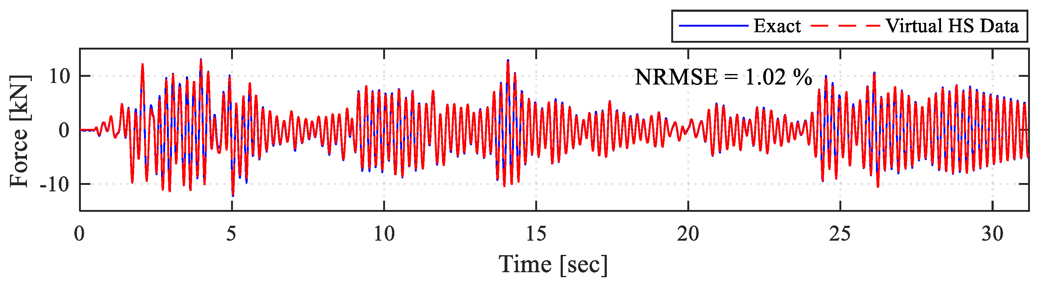
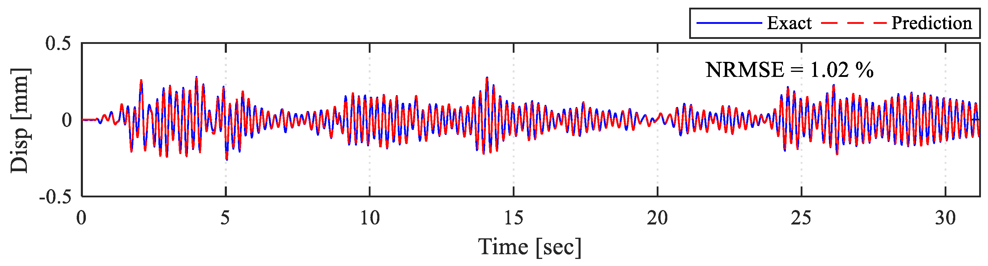
First, the virtual HS results are shown, where at each time step, linear elastic force feedback was calculated and fed back to the deep learning model (i.e., analytical substructure). This case can be considered as a coupled LSTM-FE model. Figure 11 shows the brace displacement time history comparison for LSTM prediction and the exact displacement. It can be seen that the model predictions are accurate enough for a stable and accurate virtual HS analysis. Moreover, Figure 12 shows force time histories from the same analysis. Since virtual HS relies on pure calculation, the force time history for the virtual HS has the same behavior as the displacement prediction time histories.

Figure 13 shows the brace displacement time history for the aforementioned model, where no actual specimen is used. However, this time the LSTM model was integrated into the RTHS loop, where the actuator was free to move, and the displacement feedback was multiplied with the stiffness constant to represent linear-elastic brace response. It can be seen from the figure that the LSTM model has accurate predictions as well. 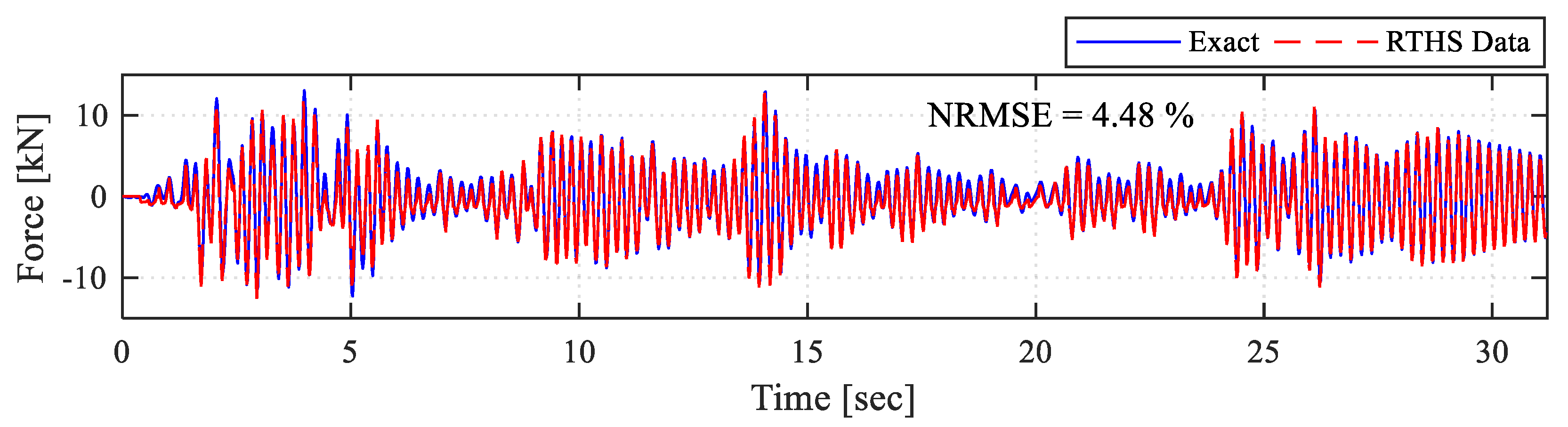Moreover, Figure 14 shows the comparison of force feedback from the experimental setup and the exact force values, which is the training input. It can be seen that the error in the obtained forces is more than the displacement prediction error. This is due to the experimental errors related to the RTHS setup, which is expected but was never quantified yet for ML-driven RTHS tests. Such errors are again the main motivation of extending the training domain when generating the Deep-LSTM models. Overall, both the training domain and the accurate predictions reflected well to the force–time histories, and the test was completed successfully with adequate accuracy.

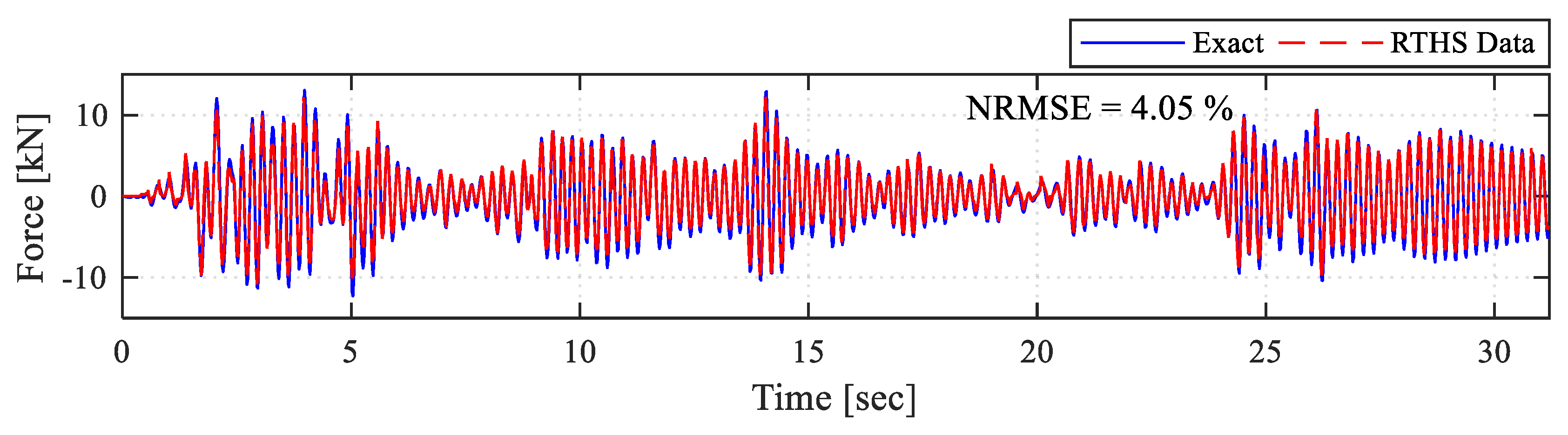
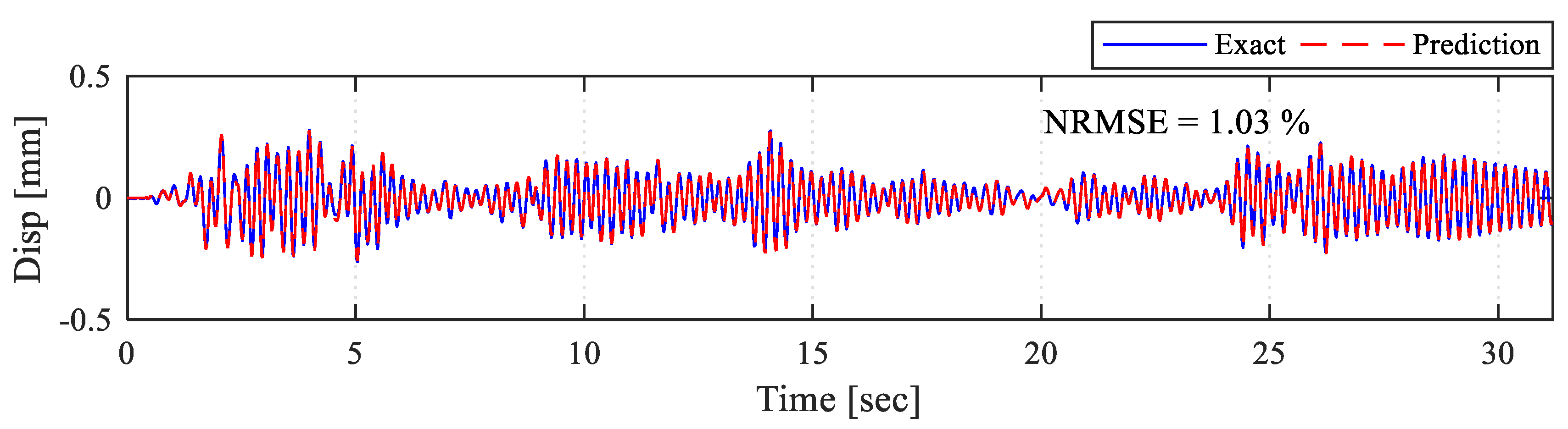
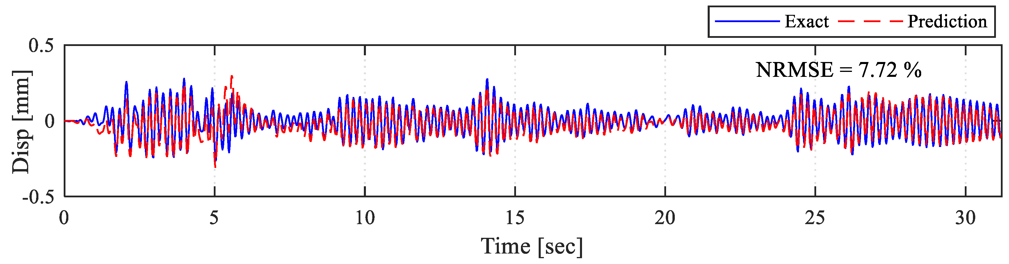
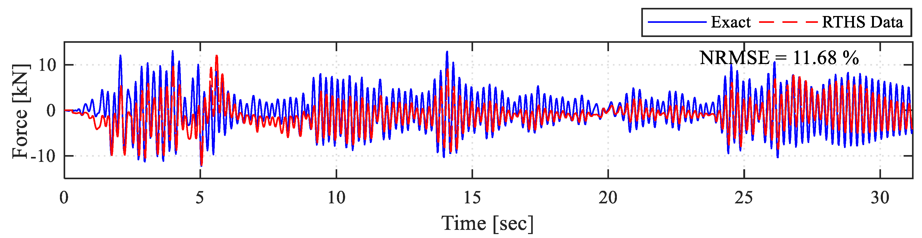
Next, the RTHS test results for the same model with the actual specimen are shown. The LSTM predicted displacement time histories are compared with the exact solution in Figure 15. It can be seen that the model predictions are the same as the previous case without specimen (average error is about 1%). Moreover, Figure 16 shows the force feedback time history response from the actual specimen. It can be seen that, with the actual specimen present, the model successfully completed the RTHS tests with relatively small error (~4.5%) similar to the case of free actuator without specimen showed above in Figure 14.

5.2.2. Selected Results from ‘Bad’ RTHS Tests

This section aims at presenting a case of successfully completed ML-driven test but with relatively large errors, which we call it a ‘bad’ test. The sample test results are from Model 1a RTHS tests when no delay compensator was used, but for using actual force feedback to update the last lookback dimension as opposed to the first dimension in the ‘good’ test in Section 5.2.1. These RTHS test results are again compared with the exact solution, which was possible to obtain from pure analytical models because of the linear elastic brace behavior. The goal here is to show that due care is needed when handling the Deep-LSTM model attributes to avoid getting large errors.

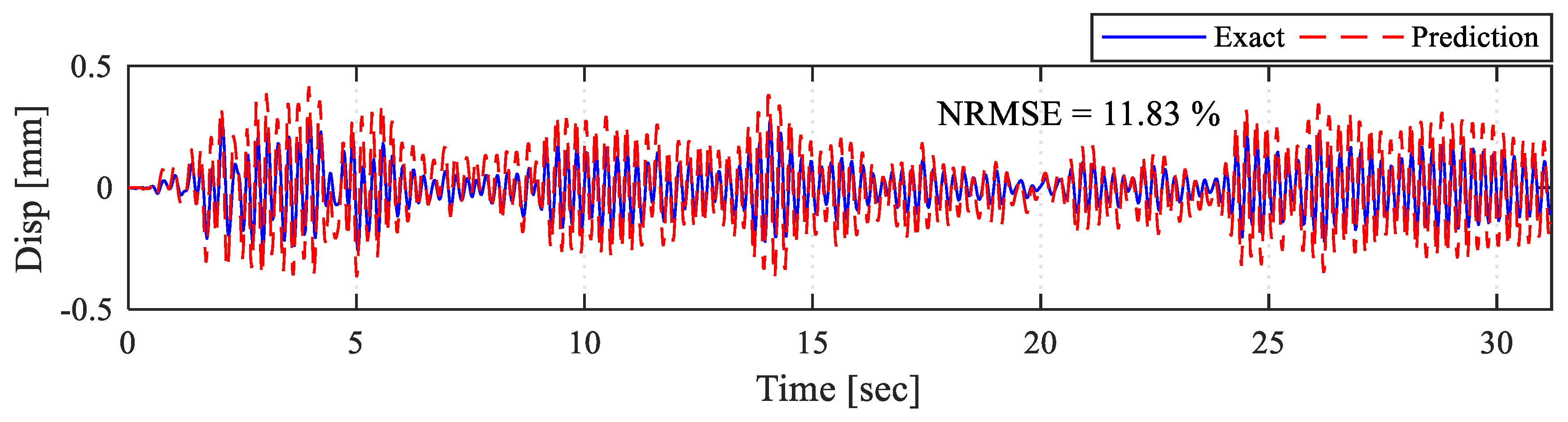
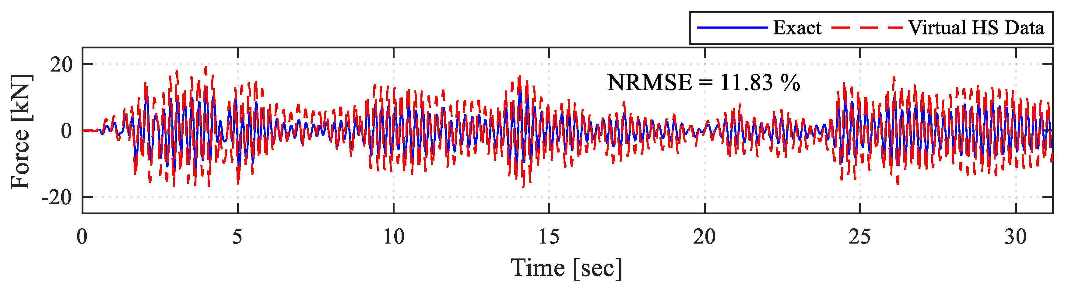
As before, the virtual HS results from coupled LSTM-FE model are shown first, where at each time step, linear elastic force feedback was calculated and fed back to the deep learning model (i.e., analytical substructure). Figure 17 shows the brace displacement time history comparison for LSTM prediction and the exact displacement. Moreover, Figure 18 shows force time histories from the same analysis. Since virtual HS relies on pure calculation, the force time history for the virtual HS has the same behavior as the displacement prediction time histories, and both showed relatively large errors of about 11.8%. Thus, the virtual HS trials could be very beneficial to consider before actual future ML-based RTHS testing to get an early sense of what model attributes will likely lead to more accurate results.

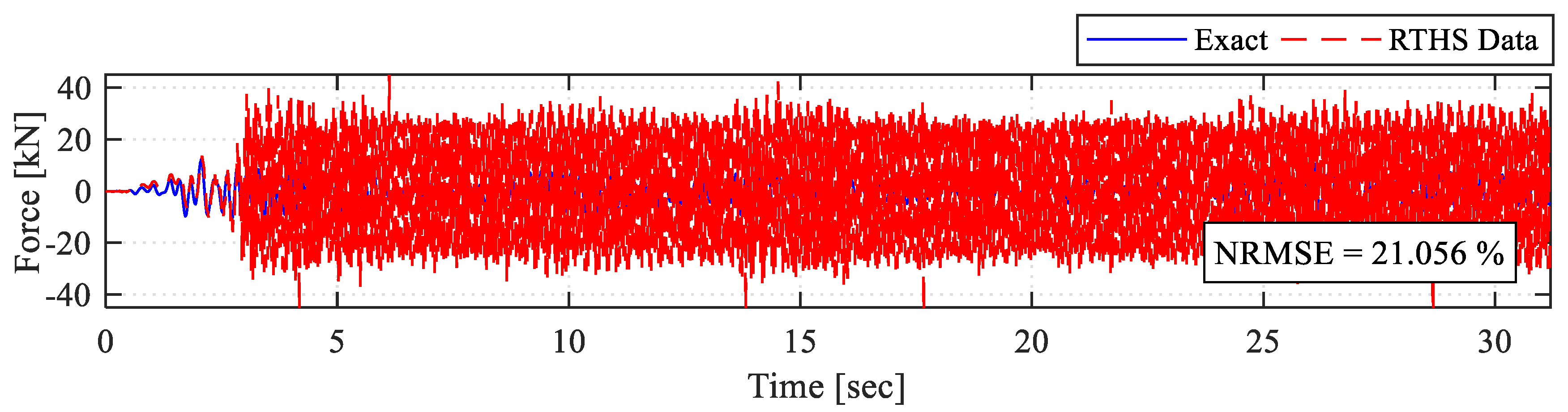
Figure 19 shows the brace displacement time history for Model 1a where no actual specimen was used. As seen from the LSTM displacement predictions, a large prediction error starts early on during the testing. These errors just kept accumulating and were further propagated because of the nature of the hardware setup which eventually led to incorrect experimental results. The force feedback obtained from the experimental setup is compared with the training force input in Figure 20. The error from the displacement prediction, which is also the actuator input command, is reflected in the force feedback as expected. When the RTHS setting did not have any delay compensator, and the force feedback was fed into the force input’s last dimension, the model predictions were not appropriate to conduct an accurate test, even though the test was still successfully executed, i.e., stable and displacements remained within the training output range.

The RTHS test results for the same case above are evaluated but now from the tests that used an actual specimen. Figure 21 shows the brace displacement prediction time histories. It can be seen that when an actual specimen is used in the HS setup, it helped stabilize and suppress the error in the early stages of the test, and in turn, no large errors accumulated and more reliable test results were obtained. Although the predictions were not still very accurate (average error dropped to about 7.7% down from 28% when no specimen was used), it provided satisfactory enough predictions that were not as noisy or contaminated with artificial high frequencies as the case with no specimen. Figure 22 shows the brace force feedback obtained in return to the predicted brace displacement. As it is seen from the force time history, the force feedback was appropriate and relevant to the displacement input. Therefore, it can be observed that including an actual specimen within the system helps improve the performance of the RTHS testing with ML/LSTM computational substructures.

5.3. Error Evaluation

The normalized root mean square errors (NRMSE) was calculated for all conducted RTHS cases (see sample values on Figure 11, Figure 12, Figure 13, Figure 14, Figure 15, Figure 16, Figure 17, Figure 18, Figure 19, Figure 20, Figure 21 and Figure 22 above). A summary of the NRMSE values from the tests that used first and last force feedback lookback dimension update is provided in

Table 1. NRMSE (%) for brace displacement predictions where ‘first’ force input dimension is updated in RTHS tests.

		Model 1		Model 2
		Model 1a	Model 1b	Model 2a	Model 2b
Virtual Hybrid Simulation		1.05	1.02	1.02	1.13
w/ATS	w/o Specimen	1.06	1.03	1.04	1.12
	w/Specimen	1.03	1.03	1.06	1.10
w/o ATS	w/o Specimen	0.97	1.02	1.02	1.12
	w/Specimen	0.93	1.02	1.02	1.11

and

Table 2. NRMSE (%) for brace displacement predictions where ‘last’ force input dimension is updated in RTHS tests.

		Model 1		Model 2
		Model 1a	Model 1b	Model 2a	Model 2b
Virtual Hybrid Simulation		11.82	5.46	10.48	13.02
w/ATS	w/o Specimen	29.78	20.85	26.32	27.16
	w/Specimen	20.02	17.39	12.07	12.94
w/o ATS	w/o Specimen	28.37	2.04	27.65	28.42
	w/Specimen	7.72	5.01	6.54	23.88

, respectively. In these tables, the brace displacement predictions are compared with the training displacement data. Before conducting the tests, virtual HS tests were conducted, where at every time step, the displacement predicted by the deep learning model and the input force was calculated from a constant stiffness multiplier. It can be seen from the results that in general, the models have more errors when the last lookback dimension is updated during the RTHS tests as opposed to the first dimension even from the virtual HS cases.

For Model 1, the error is reduced for the actual RTHS cases with physical specimen and no ATS delay compensator used. On the other hand, the error is more pronounced for Model 2 with the last dimension update. This error accumulated when the online RTHS tests were conducted as seen from the values in the table. When tests include actual specimens, this slightly helped stabilizing and reducing the error. Overall, the system performed well for all ‘first’ lookback dimension update test cases when the feedback is used for the first force input’s lookback dimension, and all these cases did not have any noise in the predictions. Another observation, which is more pronounced in Table 2, is that the use of ATS does not reduce the error in the predictions, and in fact, it might increase the error in some cases. Therefore, it can be concluded that the use of delay compensators—such as ATS—is not recommended nor needed when ML models are used for RTHS computational substructuring.

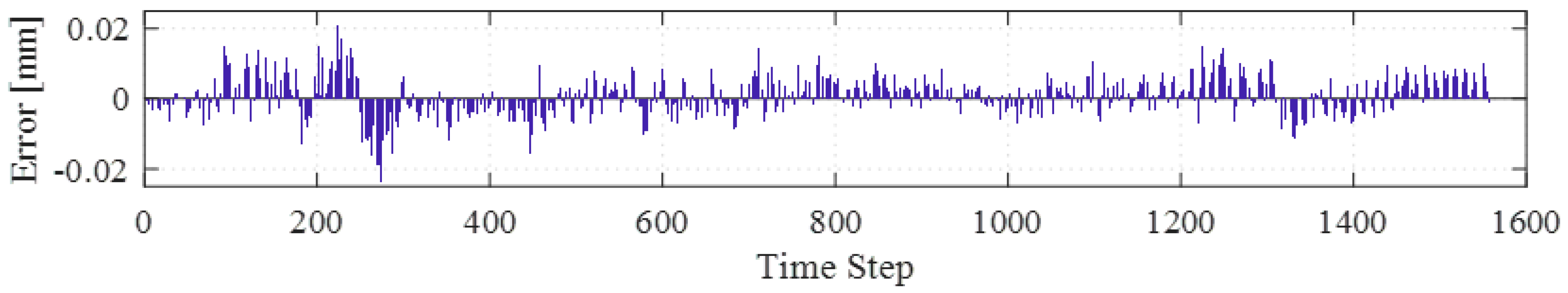
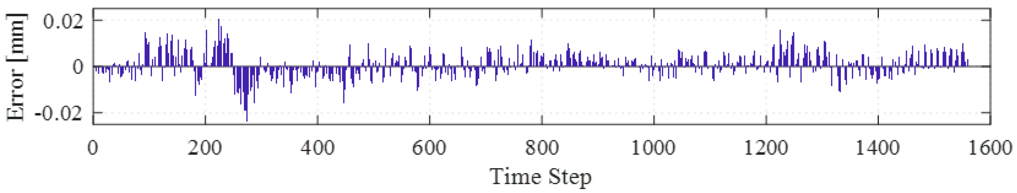
Lastly, the absolute error (in mm) at the small brace scale for each time step of the displacement prediction during the RTHS is reported for the selected models and cases presented above in Section 5.2. Figure 23 and Figure 24 show the difference between the exact displacement and displacement prediction (input for the actuator) for the sample ‘good test’ case presented in Section 5.2.1. As implied from the previously provided discussion and comparisons, the error is very small for both cases with and without specimens, and such small errors did not lead to any issues during the RTHS tests. 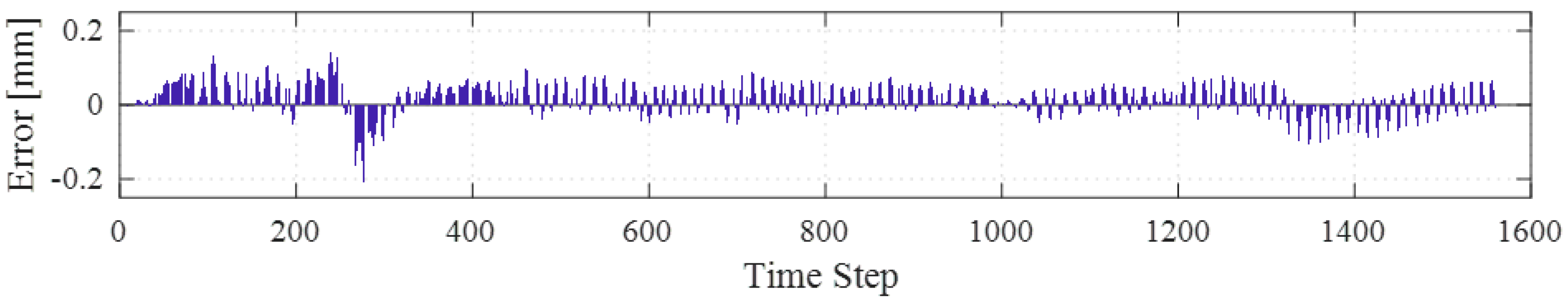On the other hand, Figure 25 and Figure 26 show the same displacement difference calculation for the ‘bad test’ example presented in Section 5.2.2. A systematic error can be observed from the case where no specimen is used. Figure 26 shows the results for the tests with actual specimen used in the loop. Although the error values are still relatively large when a specimen is included, yet it is better and much smaller than the case without specimen. That figure confirms the observation that the tests with specimen did not experience the same systematic or significant error accumulation as the ones with a free actuator.

6. Concluding Remarks

This study focused on assessing the quality of RTHS results when ML models are used to represent computational substructure behavior under dynamic excitation. Two FE models of one-bay one-story CBF were developed and used to obtain training datasets for the ML models. Deep-LSTM networks were used to develop the metamodels of the computational substructure’s response under earthquake excitation. Two different models were developed for each CBF case with 15 and 20 lookbacks. Overall, a total of 32 RTHS tests were conducted in this study. Both RTHS tests with and without an actual specimen were considered for further assessment and better understanding of test results. However, whenever an actual specimen was used in the online RTHS tests, the specimen remained linear elastic for possible evaluation against an exact analytical solution. For each RTHS case, the force feedback from the actuator was either updated in the first or the last lookback dimension of the force input. While the study provides for the first time exclusive results for ML-driven RTHS tests with physical specimens, the following major conclusions can be drawn:

• The experimental substructure response in terms of the brace force–displacement relationship was found to adequately fit within the envisioned training domain proposed herein. This confirms that it is recommended to expand the training domain to somehow account for the uncertainties associated with RTHS force–displacement dependency and errors from hardware.
• To inform and select ML model attributes for ML-driven RTHS testing, two practices are recommended with the assumption of linear elastic specimens. Either free-actuator tests, i.e., with actual hardware but without specimen, or virtual HS tests, i.e., FE simulated specimen, can be conducted. The examples from good and bad tests presented in this paper show that the virtual HS tests can be more revealing. In either way, careful model tuning or parameter identification—e.g., LSTM lookback dimension update—should be considered since the ML prediction error can quickly propagate and accumulate with the experimental errors.
• By inspecting force and displacement time histories from RTHS tests with LSTM models, it was observed that RTHS with actual specimen, which is the more realistic case, showed less error accumulations and better predictions. In other words, test specimens help stabilize and reduce experimental errors in the tested cases. Thus, error predictions from virtual HS or free-actuator testing will provide correct trends on model attributes and performance, but will likely get smaller during actual tests with specimens.
• Based on results from 32 tests and utilized test setup, it can be demonstrated that using ML models within the RTHS loop for analytical substructuring can eliminate the need for actuator delay compensators. This is because the models can be trained with inherent delay beforehand. However, more testing scenarios, different hardware and laboratory setups, etc. should be considered for future studies before a solid reliable recommendation can be made in this regard.
• Overall, NL-driven RTHS tests performed well when deep learning metamodels were used to represent the analytical substructure dynamic behavior, and no stability issues were observed. The study also highlighted that the accuracy of test results could be affected by the nature of the LSTM model update during the test. For example, the models where the first lookback dimension is updated, as opposed to last one, performed better. Thus, more future research is also recommended to study ML modeling features and parameters sensitivity as it pertains to RTHS performance, and extend this concept to nonlinear physical specimens, where deep learning models need to be trained based on complex unknown behavior.