Abstract
Forest structure estimation is very important in geological, ecological and environmental studies. It provides the basis for the carbon stock estimation and effective means of sequestration of carbon sources and sinks. Multiple parameters are used to estimate the forest structure like above ground biomass, leaf area index and diameter at breast height. Among all these parameters, vegetation height has unique standing. In addition to forest structure estimation it provides the insight into long term historical changes and the estimates of stand age of the forests as well. There are multiple techniques available to estimate the canopy height. Light detection and ranging (LiDAR) based methods, being the accurate and useful ones, are very expensive to obtain and have no global coverage. There is a need to establish a mechanism to estimate the canopy height using freely available satellite imagery like Landsat images. Multiple studies are available which contribute in this area. The majority use Landsat images with random forest models. Although random forest based models are widely used in remote sensing applications, they lack the ability to utilize the spatial association of neighboring pixels in modeling process. In this research work, we define Convolutional Neural Network based model and analyze that model for three test configurations. We replicate the random forest based setup of Grant et al., which is a similar state-of-the-art study, and compare our results and show that the convolutional neural networks (CNN) based models not only capture the spatial association of neighboring pixels but also outperform the state-of-the-art.
1. Introduction
Estimation of forest’s structure is of immense importance in geological, ecological and environmental studies. Carbondioxide, one of the constituents in the atmosphere, plays a vital role in the life cycle on the planet. It is consumed by plants, via photosynthesis, to generate food contents and oxygen. However, due to global industrial revolution, carbondioxide is constantly being pumped into the atomosphere, resulting in rising levels. The level of carbondioxide has increased from 280 ppm, before the industrial age, to around 390 ppm in 2012 and now it has risen to a value of around 407 ppm [1]. To provide a fair perspective, this value has not gone above 300 ppm in the past 800,000 years. Due to its contribution in green house effects, this rising level of carbondioxide is resulting in a rise of average global temperatures. Keeping this burning issue of global warming in focus, the carbon stock estimation at multiple scales has become a critical parameter [2]. Assessment of forest’s structure directly yields the estimate of carbon stock. The analysis of global carbon cycle is directly related to the variations in percentage coverage of the forests and can be used to manage the sequestration and carbon-sources/carbon-sinks [3,4]. Furthermore, the forest covering and its variations have a direct impact on the diversity of ecosystems. The severe consequences of deforestation on the environment and ecosystems make the problem of forest structure estimation important to discover. Multiple parameters are being used to quantify the forest structures for the estimation of carbon biomass. The noteworthy parameters are tree height, diameter at breast height (DBH), species of trees, age of trees, leaf area index (LAI), vegetation height, above ground biomass (AGB), canopy gap size and fractional cover [5,6,7,8]. The vegetation height is of particular importance here because it provides the basis for the long term change analysis of forest regions [9,10] and when combined with species information and site quality, it can be used to get the educated estimates of stand age and successional stages [11]. The method of in situ surveys provides accurate figures at ground level based on statistical sampling of the geographical region under study. Although accurate, this method is not feasible because it requires a huge amount of resources in terms of manpower, time and cost for complete spatial coverage and is susceptible to the area’s accessibility and human related errors at large scale estimations. The method, even with its limited scope, is used to perform the calibrations and evaluations of more automated techniques developed for this task [12].
Light detection and ranging (LiDAR) imaging provides an accurate mechanism to develop the 3D models of the target. In this imaging mechanism, the LASER light is shot at a target in pulses and the reflected light is received by a receiver. The reflection of light from variable distance causes it to arrive at the receiver at slightly different times, and this difference in time is then converted into distance which is then converted into high resolution three dimensional model of the target. LiDAR is proved to be a useful tool to assess and manage the damages of natural disasters [13]. It is used in a wide array of applications in forestry like large-scale forest inventory management, biophysical monitoring of forests and biomass estimation [14,15,16]. It provides accurate means to map the canopy height and has been used for this purpose several times [17,18,19]. The usefulness of LiDAR data in remote sensing applications cannot be undermined, however, this data (when requested on-demand) is expensive to obtain and does not have global coverage. There is a need to establish a mechanism to estimate the height of vegetation using globally available and low cost (or even free) satellite data with the assistance of available LiDAR data. In this work, we utilize the deep convolutional network to relate the Landsat images with LiDAR data. This estimated mapping is then used to estimate the digital canopy height through Landsat imagery only. Because the Landsat data has global coverage with a massive database and is freely available, its utilization in digital canopy height estimation can provide a very cheap alternative to expensive and hard to obtain LiDAR data.
Multiple studies have established the relationship between Landsat imagery and in situ measurements like fractional cover [20], above earth woody vegetation biomass [21,22,23] and leaf area index [24,25]. Some of these techniques utilize statistical techniques like linear and non-linear regression models of single or multiple attributes while others incorporate machine learning techniques, both supervised and unsupervised. Researchers have used the depth information from LiDAR data and mapped it to Landsat data using statistical models to enhance spatiotemporal coverage [26,27,28,29,30]. Wilkes et al. utilize LiDAR derived canopy height in combination with a composite of Landsat imagery with Moderate Resolution Imaging Spectroradiometer (MODIS) to estimate the canopy height using random forest regression model [31]. Some use the composite of Landsat data with other sensors in combination with LiDAR data to estimate the canopy height [31,32,33] while others focus on the utilization of Landsat imagery only in combination with LiDAR data [33,34]. The common attribute of all these works is that they use the random forest ensemble regression model.
The random forest machine learning ensemble algorithm is quite famous among remote sensing experts [31,35,36,37,38] due to its ease of use, high non-linearity and robustness to outliers in training data. Pal et al. classify seven classes of land covers in enhanced thematic mapper sensor data using random forest models [35]. Mellor et al. utilize random forest models on thematic mapper sensor data in combination with auxillary terrain data and climate attributes to classify between forest/non-forest class [36]. Others have used random forest models for carbon mapping and above ground biomass estimation [31,37,38]. Besides the popularity of random forest model among the experts, the inherent shortcoming of random forest regressor, with reference to spatial data, is that it does not utilize the spatial associations of landcover in satellite data. They make the prediction of single location by treating each input point independently. To exploit the mutual dependence of neighboring landcovers, we use the convolutional neural networks (CNN) with Landsat and LiDAR data to estimate the digital canopy height of the region under study. The proposed network predicts the canopy height with mean absolute error of 3.092 m and variance of 0.864 m, outperforming the state-of-the-art.
2. Proposed Solution
In this research work, we are using the Landsat images in combination with digital canopy height extracted from airborne LiDAR data in the area located near Flagstaff, Arizona. While previous studies use similar or the same combination of types of data for canopy height estimation, they select the random forest ensemble model for prediction. Because this algorithm utilizes the pixel-to-pixel mapping to establish the model, it inherently loses the useful information of spatial relationship between the neighboring land covers. As the remote sensing data is spatial in nature, our assumption is that the neighboring land covers are associated with each other and do encode useful information, when processed together. Keeping this in view, we propose the utilization of the deep CNN model for estimation of vegetation height. These deep learning models have the capabilities to unravel the hidden spatial patterns along with the radiometric associations of input (Landsat images in this case) with the target data (LiDAR data in this case). To our knowledge, CNNs have never been used before for the estimation of canopy height from Landsat and LiDAR data. We adopt a five stepped approach. (1) data preprocessing (2) feature selection (3) model selection and training (4) inference (5) comparison with recent similar work.
3. Study Area and Data
3.1. Study Area
This study is conducted in the area on the west and north west of Flagstaff, Arizona. This region falls in the area of Coconino National Forest Flagstaff, Arizona. Coconino national forest spans a total area of 1.85 million acres. The average annual temperature of the forest is 8 C. Average annual rainfall precipitation is mm and average snowfall is cm. This forest is home to various tree species, especially Ponderosa pines, Limber pine, Single leaf pinyon pine, Arizona cypress and many others [39]. The type of vegetation in this forest is dependent upon the elevation. At lowest elevations (4500 feet to 6500 feet), the forest is mainly covered in sagebrushes and small shrubs. In elevations between 6500 feet and 8000 feet, the majority of the area is covered by Ponderosa pine (average height of 37 m) [40]. Our area of study falls in this elevation bracket. Other species situated in the region of study are Rocky Mountain juniper (average height of 15 m), quaking aspen (average height of 23 m) and Gambel oak (average height of 6 m). Table 1 shows the percentage coverage of the type of trees in the study area. The maps shown in the Figure 1 display the area under study. The left image shows the false color composite of Landsat data and the right image shows the corresponding canopy height model.

Table 1.
Landcover types and percentage in area of study.
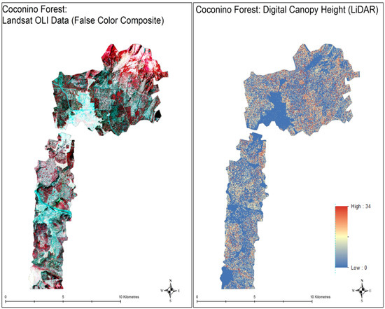
Figure 1.
Map of study area. The left image is the false composite image of area under study and the right image is the digital canopy height generated from the light detection and ranging (LiDAR) data obtained from OpenTopography [41]. The Landsat data not only contain 11 bands of Landsat 8 but also contain 19 normalized and direct band ratios.
LiDAR Data
The LiDAR data used in this study is freely available on https://opentopo.sdsc.edu and was collected on 16 October 2017 for Jonathan Donager, Northern Arizona University, School of Earth Sciences and Environmental Sustainability to study the forest structure changes and its influence on snowpack persistence and accumulation [41]. The data was gathered by National Center for Airborne Laser Mapping (NCALM) as seed grant. The Raster resolution of this data is and the point cloud density is . The digital elevation model (DEM) and digital terrain model (DTM) derived from this data are used to compute the canopy height model (CHM) to be used in this study. Figure 1 displays the CHM map for the area under study. The data is resampled to match the spatial resolution of Landsat data using nearest pixel settings. The height of the canopy ranges from 0 m to 34 m.
3.2. Landsat Data
The Landsat data is chosen in such a way that it falls as close to the date of acquisition of LiDAR data as possible to minimize the temporal changes. The cloud free operational land imager (OLI) data of the area of interest is available for 3 October 2017 and is selected for this study. The path/row of the data is 37/36. The OLI sensor provides the data with spatial resolution of 30 m and radiometric resolution of 16 bit. The OLI sensor is mounted on the Landsat 8 satellite which revisits the given area every 16 days.
3.3. Feature Construction
Generally the deep learning models are known for their capability to mine the complex patterns in the given data without the need of feature engineering, however, it is recommended to have some features engineered as per domain knowledge. This results in relatively simpler models and also contributes to faster convergence. Studies have shown that different vegetation indices and band ratios are correlated with different canopy types and heights [34]. We take the head start from the work of Grant et el. and calculate a total of 19 vegetation indices and band ratios mentioned in their study [34]. We stack these features with Landsat imagery. Table 2 provides the list of constructed indices as features. Indexes 1 to 11 are for Landsat original bands. Indexes 12 to 30 are defined in Table 2.
Table 2.
The list of used vegetation indices and simple band ratios.
4. Methodology
We utilized the Landsat bands and selected vegetation indices stacked together as the input and the corresponding canopy height image as the target to the model. The digital canopy height image was down-sampled to match the spatial resolution of Landsat imagery using nearest pixels settings. The following step-wise approach was followed for the training process.
- Data preprocessing and partitioning.
- Feature selection.
- CNN model development and training.
4.1. Data Preprocessing and Partitioning
The input Landsat and the target canopy height images are divided into 30 × 30 pixel image tiles with no overlap. The dataset forms a total of 87 (30 × 30) images. Both input and target images are normalized using min-max scaler and then partitioned into training and test set by the 70:30 ratio. The training dataset is further partitioned into training and validation set by ratio of 85:15. The training data is used to train the model and is validated via validation dataset on each training epoch. The test dataset is then used to model the generalization error. Figure 2 displays the true CHM of test data set and shows that the test dataset is evenly distributed over the whole study region.
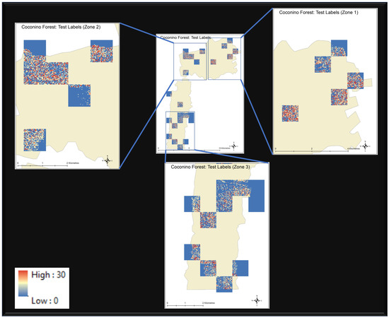
Figure 2.
Visual interpretation of test data set distribution over the area of study. The rest of the area (not covered by these tiles) makes the training data.
4.2. Feature Selection
Every single feature serves a specific purpose in the bigger domain of remote sensing applications. The red, green and blue bands, which lie in visible region of spectrum, provide the visual interpretation of what we see on the ground. Short Wave Infrared bands (SWIR) can penetrate thin clouds and discriminate moisture content of soil and vegetation. Near Infrared band (NIR) is highly responsive to chlorophyll contents. These different bands, when combined in a specific manner, can lead to completely new interpretations. Normalized Difference Vegetation Index (NDVI), which is derived from NIR and Red band, provides pretty good estimation of biomass. Normalized Burn Ratio (NBR), which is derived from NIR and SWIR, is used to estimate fire severity and highlight recently burned areas. NDVI and NBR are two of the many good examples of how multiple bands can be combined in different ways for different applications. The idea is to explore the option of combining all the features together to form a complex composite input and feed it to deep learning algorithms which are known for handling complex input–output relationships to see if it can model the relation between Landsat data and canopy height or not. Three approaches are followed in the feature selection process and then compared. In the first approach, all the 30 features are stacked together as bands and used in training. In the second approach, the features selected by [34] are used to train the CNN. Figure 3 represents the features selected by [34].
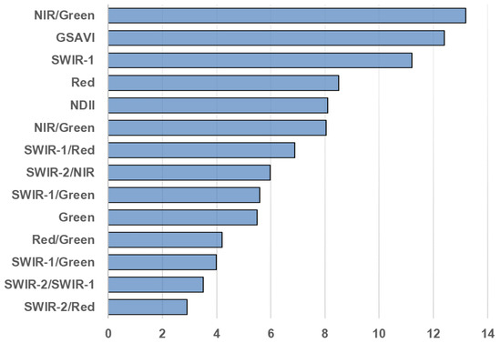
Figure 3.
Relative importance score of feature in [34].
In the third approach, individual features (selected bands, band ratios and vegetation indices) are assessed one-by-one using CNN training and are ranked based on validation mean square error. Figure 4 displays the features with their usefulness. Once the features are enlisted based on their usefulness, a threshold is defined on feature score to remove the “less useful” features. Features in Figure 3 do not match with features in Figure 4 or have different ranking placement. There are three major factors that may cause this difference. First, geographical locations of areas under study are very different. Second, types of vegetation under study are different and third, the mechanism to select features in the two studies is very different.
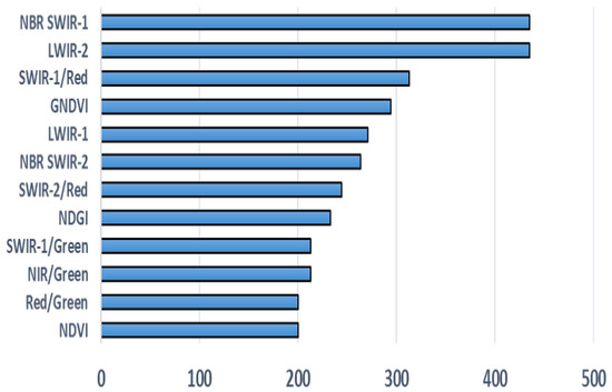
Figure 4.
CNN based feature usefulness score.
4.3. CNN Model Development
CNNs have drawn enough attention for their applications in image identification and signal processing [42,43] and are being used in remote sensing applications like road network extraction [44], vehicle detection [45], semantic segmentation [46] and scenario classification [47]. CNNs are capable of unraveling the hidden patterns in image data. Besides pixel to pixel intensity association, CNNs utilize spatial association of neighboring pixels for classification and regression tasks. Using the combinations of convolutional layers and max pooling layers, CNN gets enhanced accuracy in classification tasks and usually outperforms the traditional machine learning models like support vector machines and random forests [48,49]. CNNs have several major components i.e., convolutional layers, pooling layers, dropout layers and fully connected layers. The convolutional layers, in assistance with pooling layers, are responsible for feature extraction at different scales in the image. Fully connected layers utilize those features for regression or classification.
For this research work, we experimented with multiple configurations of the CNNs and after comprehensive testing process we proposed the network architecture shown in Figure 5. The network takes image as input where N is the total number of bands. There are four convolutional layers in the network. The first layer extracts 256 features from the input data at full resolution. The result of the first layer is fed to the second convolutional layer which extracts 8 features from its input image. The third layer extracts 16 features whereas the fourth (and the last layer) extracts one feature image which is then passed through linear activation function. We have bypassed the fully connected layer and the result of the linear activation layer is considered the target image. We use drop out of at first layer to avoid the overfitting problem. Each layer is followed by batch normalization and activation function of rectified linear unit (ReLu) except the final layer (for which the activation is linear). The stochastic gradient descent function is used for training with the Mean Absolute Error (MAE) as loss function as shown in (1). We utilize the MAE as loss metric to be able to make a fair comparison with [34].
where is the canopy height model derived from LiDAR data, M is number of pixels in the image (=900 in this case) and is the predicted average canopy height model by the network.
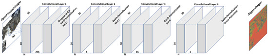
Figure 5.
Our designed CNN. Here N is the number of features (bands and band ratios) in the input Landsat data.
4.4. Network Training
Four approaches are followed for the training process of CNN. In the first test case, all 30 features (11 bands and 19 band ratios and vegetation indices) are utilized in the training process. In the second test case, the features are selected by [34] with selected CNN model. Grant et al. utilized the SciKit Learn [50] random forest default feature selection model in their study so in the third test case, those features are tested with random forest regression model with identical settings adopted by Grant et al. In the fourth test case, we train and analyze the model using the features selected by the CNN based procedure and the results are compared.
4.4.1. Test Case 1: Training with All the Features
In this approach, the Landsat data with all the bands along with the selected band ratios and vegetation indices discussed in Section 3.3 are stacked together to form a total of 30 band images. With canopy height image as the target output, the network is trained to minimize the mean absolute error between prediction and known output.
4.4.2. Test Case 2: Training with Features Selected by Grant et al.
In order to cope with the overfitting in the first test case, it is important to select the useful features before training the model. Grant et al. in their research [34] ranked the features discussed in Section 3.3 based on their usability score. They used the Scikit-Learn random forest library’s default feature scoring mechanism to rank the features [50]. In this test case, we test our network by training using the features selected according to [34] to see if it has any benefit in training or not. The selected features are used to trained our proposed CNN model.
4.4.3. Test Case 3: Training with Features, Selected by Grant et al., Using Random Forest Regression Model
Because the features in the previous test case are selected specifically for random forest models, we test these features using random forest regression instead of our proposed CNN architecture. We train the random forest model with the identical settings described in [34] for comparison.
4.4.4. Test Case 4: Training with Features Selected by CNN Based Feature Selection Method
In this test case, we determine the feature usability score for CNN by analyzing each feature individually. Each feature is used to train a simple CNN based model for 2000 epochs and then ranked based on least mean square validation error. The reciprocal of this error is taken as the score of usefulness. Figure 4 shows the usefulness score of the feature in descending order. We take all the features with score greater than or equal to 200 and use them in the training process of the final CNN model.
5. Results and Discussion
5.1. Test Case 1: Training with All Features
CNN model is trained with all the available features in this approach. With canopy height image as the target output, the network is trained to minimize the mean absolute error between prediction and known output. Figure 6 shows a training and evaluation graph for the training process. It is visible from the graph that the training error decreases with increasing epochs and gets as low as 0.085 (2.89 m) but the validation error stays at 0.1 (3.4 m). This gap in the training and validation error suggests that the model is overfitting.
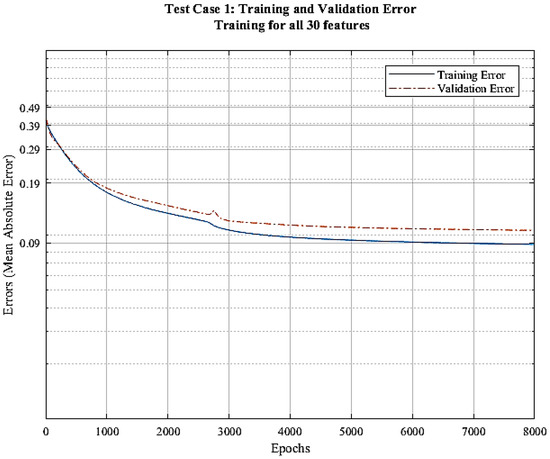
Figure 6.
Error vs. epochs graph for test case 1.
5.2. Test Case 2: Training with Features Selected by Grant et al.
In this approach, we select features in order to avoid overfitting. We select features according to criteria mentioned in [34]. There seems to be no improvements in the training process when the features selected from the research in [34] are utilized. The consistent gap in the training and validation errors clearly indicates that the model is still overfitting. This is probably due to the fact that these features are scored based on their performance on random forest regression algorithm and are not suited to be used for CNN. Figure 7 displays the training and validation error of the process vs. epochs.
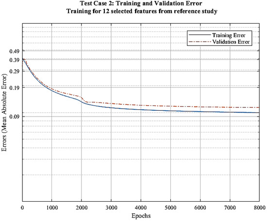
Figure 7.
Error vs. epochs graph for test case 2.
5.3. Test Case 3: Training with Features, Selected by Grant et al., Using Random Forest Regression Model
We use the same features as discussed in the previous test case and develop a random forest regression model instead of our proposed CNN model. We use the identical settings for random forest described in [34] for comparison. With the selected features and the settings, the trained model has the accuracy of 0.0202 (0.68 m) in terms of mean squared error and 0.068 (2.33 m) in terms of mean absolute error but the variance is very high i.e., 0.1522 (5.17 m). This suggests that for random forest based regression model, the selected features in [34] may not be independent and may vary from dataset to dataset.
5.4. Test Case 4: Training with Features Selected by CNN Based Feature Selection Method
In the last case, we determine the features’ usefulness score for our proposed CNN model. Figure 4 shows the usefulness score of the feature in descending order. We select all the features with score greater than or equal to 200 and use them in the training process of the final CNN model. Figure 8 displays the training and validation error vs. epoch curves. The training and validation error decreases down to 0.085 (2.89 m) and 0.0904 (3.092 m).
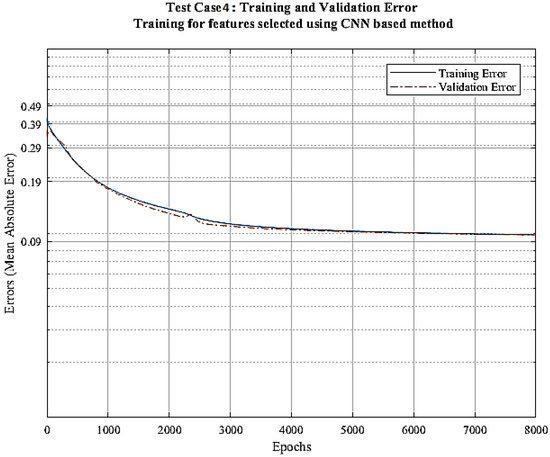
Figure 8.
Error vs. epochs graph for test case 4.
5.5. Discussion
For the test case 1, when all the features are selected for training, the mean absolute error for test data is 3.65 m, mean square error is 1.05 m with the variance is 1.009 m. When the features selected in [34] are assessed with CNN in test case 2, the mean absolute error is 3.43 m and mean squared error is 0.98 m with the variance of 0.923. These test data results are better than the test case 1 but the consistent gap between training and validation error graph in Figure 7 suggests that the model is overfitting. In the third test case, when we train the random forest with the features selected in [34], we get the model with mean absolute error of 2.33 m and mean square error of 0.686 m with the variance of 5.168. In terms of test error, this model is better but the confidence is too low because of very high variance. These results suggest that for the random forest model, the feature selection method is dependent on the data and may need to be repeated for the data for new regions. Among all the configurations tested, the test case 4, i.e., CNN model with the features selected based on the CNN based techniques, provides the best accuracy in terms of errors and confidence in inference. The model provides the predictions with the mean absolute error of 3.092 m, mean squared error of 0.8872 m and the variance of 0.864 m. Table 3 summarizes the accuracy of all the configurations on test data. Figure 9 visually compares the predictions of our CNN model with the true canopy height model. It can be seen in the predicted images that the CNN tends to smooth out spatial details in the image but this can be improved by more training samples and relatively complex models. Keeping in view the limited computational resources and available training data, we limit the complexity of the model in this study. It is evident from the results that the CNN does exploit the spatial association of pixels while predicting the canopy height from Landsat imagery.
Table 3.
Result comparison table for the four test cases.
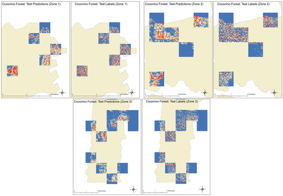
Figure 9.
Visual comparison of predicted and actual canopy heights in different zones of area under study.
6. Conclusions and Future Work
In this research work, we utilize the combination of Landsat imagery and LiDAR derived digital canopy height model to develop a deep learning model to predict the canopy height from Landsat data only. Literature is available with similar work. Grant et al. propose the solution for the same problem in their research work [34]. They utilize the random forest ensemble regression model to make the predictor. Our hypothesis is that random forest model is good in solving remote sensing related problems, however, it is inherently incapable of exploiting the spatial associations of neighboring pixels. In this work, we have proposed the usage of convolutional neural networks to develop the deep learning model to predict the canopy height using Landsat data only. CNNs not only associate the values of inputs to targets but also take into account the spatial structures in neighboring pixels for training and inference. We conducted comprehensive testing and came up with a suitable CNN structure. Inspired by the work in [34], we engineered a total of 19 vegetation indices and band ratios. We tested multiple approaches to verify multiple feature selection methods and showed that the feature selection using simple CNN based method works for CNN based models. For the given data, we compared our work with random forest based model defined in [34] and showed that our model outperforms the random forest model in terms of decision confidence. One of the limitations of deep learning methods is that they require huge amounts of data and computational power for successful implementation. In the absence of enough data, a heavy regularization penalty needs to be applied in order to avoid the overfitting problem. Furthermore, it is observed that the (automatic) selection of optimum features varies on a case to case basis, i.e., the feature selection method, adopted by researchers in [34], in our area of study does not guarantee the selection of the same features because of the difference in vegetation type and geographical location. The complexity of the model was kept relatively low due to limited computational resources, however, for future work, we are planning to increase the diversity in training along with the complexity of the model to get even better accuracy.
Author Contributions
Conceptualization, S.A.A.S.; Data curation, S.A.A.S.; Methodology, S.A.A.S. and M.A.M.; Software, S.A.A.S.; Supervision, A.B.; Validation, M.A.M.; Writing—original draft, S.A.A.S. and M.A.M.; Writing—review & editing, A.B. All authors have read and agreed to the published version of the manuscript.
Funding
This research received no external funding.
Acknowledgments
I would like to extend my gratitude to Joseph Piwowar, in Department of Geography and Environmental Studies, University of Regina for his technical expertise and feedback which helped me make significant improvements in this work.
Conflicts of Interest
The authors declare no conflict of interest.
References
- National Oceanic and Atmospheric Administration. Science and Information of Climate-Smart Nation. 2020. Available online: Climate.gov (accessed on 2 February 2020).
- Boudreau, J.; Nelson, R.F.; Margolis, H.A.; Beaudoin, A.; Guindon, L.; Kimes, D.S. Regional aboveground forest biomass using airborne and spaceborne LiDAR in Québec. Remote Sens. Environ. 2008, 112, 3876–3890. [Google Scholar] [CrossRef]
- Hamburg, S.P.; Zamolodchikov, D.G.; Korovin, G.N.; Nefedjev, V.V.; Utkin, A.I.; Gulbe, J.I.; Gulbe, T.A. Estimating the carbon content of Russian forests; a comparison of phytomass/volume and allometric projections. Mitig. Adapt. Strateg. Glob. Chang. 1997, 2, 247–265. [Google Scholar] [CrossRef]
- Ding, H.; Nunes, P.A.; Teelucksingh, S.S. European Forests and Carbon Sequestration Services: An Economic Assessment of Climate Change Impacts; Nota di Lavoro-Fondazione Eni Enrico Mattei (FEEM): Milan, Italy, 2010. [Google Scholar]
- Botkin, D.B.; Simpson, L.G. Biomass of the North American boreal forest: A step toward accurate global measures. Biogeochemistry 1990, 9, 161–174. [Google Scholar]
- Botkin, D.B.; Simpson, L.G.; Nisbet, R.A. Biomass and carbon storage of the North American deciduous forest. Biogeochemistry 1993, 20, 1–17. [Google Scholar] [CrossRef]
- Jenkins, J.C.; Chojnacky, D.C.; Heath, L.S.; Birdsey, R.A. National-scale biomass estimators for United States tree species. For. Sci. 2003, 49, 12–35. [Google Scholar]
- Centre, P.F.; Penner, M. Canada’s Forest Biomass Resources: Deriving Estimates from Canada’s Forest Inventory; Pacific Forestry Centre Victoria: Victoria, BC, Canada, 1997; Volume 370. [Google Scholar]
- Maron, M.; Gordon, A.; Mackey, B.G. Agree on biodiversity metrics to track from space. Nature 2015, 523, 403–405. [Google Scholar]
- Cook, G.D.; Liedloff, A.C.; Cuff, N.J.; Brocklehurst, P.S.; Williams, R.J. Stocks and dynamics of carbon in trees across a rainfall gradient in a tropical savanna. Austral Ecol. 2015, 40, 845–856. [Google Scholar] [CrossRef]
- Stojanova, D.; Panov, P.; Gjorgjioski, V.; Kobler, A.; Džeroski, S. Estimating vegetation height and canopy cover from remotely sensed data with machine learning. Ecol. Inform. 2010, 5, 256–266. [Google Scholar] [CrossRef]
- Yu, Y.; Saatchi, S.; Heath, L.S.; LaPoint, E.; Myneni, R.; Knyazikhin, Y. Regional distribution of forest height and biomass from multisensor data fusion. J. Geophys. Res. Biogeosci. 2010, 115. [Google Scholar] [CrossRef]
- Axel, C.; van Aardt, J.A.N. Building damage assessment using airborne lidar. J. Appl. Remote Sens. 2017, 11, 1–17. [Google Scholar] [CrossRef]
- Næsset, E. Airborne laser scanning as a method in operational forest inventory: Status of accuracy assessments accomplished in Scandinavia. Scand. J. For. Res. 2007, 22, 433–442. [Google Scholar] [CrossRef]
- Næsset, E. Practical large-scale forest stand inventory using a small-footprint airborne scanning laser. Scand. J. For. Res. 2004, 19, 164–179. [Google Scholar] [CrossRef]
- Thomas, V.; Treitz, P.; McCaughey, J.; Morrison, I. Mapping stand-level forest biophysical variables for a mixedwood boreal forest using LiDAR: An examination of scanning density. Can. J. For. Res. 2006, 36, 34–47. [Google Scholar] [CrossRef]
- Nelson, R.; Short, A.; Valenti, M. Measuring biomass and carbon in Delaware using an airborne profiling LiDAR. Scand. J. For. Res. 2004, 19, 500–511. [Google Scholar] [CrossRef]
- Næsset, E.; Gobakken, T. Estimation of above-and below-ground biomass across regions of the boreal forest zone using airborne laser. Remote Sens. Environ. 2008, 112, 3079–3090. [Google Scholar] [CrossRef]
- Drake, J.B.; Dubayah, R.O.; Knox, R.G.; Clark, D.B.; Blair, J.B. Sensitivity of large-footprint lidar to canopy structure and biomass in a neotropical rainforest. Remote Sens. Environ. 2002, 81, 378–392. [Google Scholar] [CrossRef]
- Scarth, P.; Röder, A.; Schmidt, M.; Denham, R. Tracking grazing pressure and climate interaction—The role of Landsat fractional cover in time series analysis. In Proceedings of the 15th Australasian Remote Sensing and Photogrammetry Conference, Alice Springs, Australia, 13–17 September 2010; pp. 13–17. [Google Scholar]
- Foody, G.M.; Boyd, D.S.; Cutler, M.E. Predictive relations of tropical forest biomass from Landsat TM data and their transferability between regions. Remote Sens. Environ. 2003, 85, 463–474. [Google Scholar] [CrossRef]
- Powell, S.L.; Cohen, W.B.; Healey, S.P.; Kennedy, R.E.; Moisen, G.G.; Pierce, K.B.; Ohmann, J.L. Quantification of live aboveground forest biomass dynamics with Landsat time-series and field inventory data: A comparison of empirical modeling approaches. Remote Sens. Environ. 2010, 114, 1053–1068. [Google Scholar] [CrossRef]
- Avitabile, V.; Baccini, A.; Friedl, M.A.; Schmullius, C. Capabilities and limitations of Landsat and land cover data for aboveground woody biomass estimation of Uganda. Remote Sens. Environ. 2012, 117, 366–380. [Google Scholar] [CrossRef]
- Coops, N.; Delahaye, A.; Pook, E. Estimation of eucalypt forest leaf area index on the south coast of New South Wales using Landsat MSS data. Aust. J. Bot. 1997, 45, 757–769. [Google Scholar] [CrossRef]
- Eriksson, H.M.; Eklundh, L.; Kuusk, A.; Nilson, T. Impact of understory vegetation on forest canopy reflectance and remotely sensed LAI estimates. Remote Sens. Environ. 2006, 103, 408–418. [Google Scholar] [CrossRef]
- Hudak, A.T.; Lefsky, M.A.; Cohen, W.B.; Berterretche, M. Integration of LiDAR and Landsat ETM+ data for estimating and mapping forest canopy height. Remote Sens. Environ. 2002, 82, 397–416. [Google Scholar] [CrossRef]
- Pascual, C.; Garcia-Abril, A.; Cohen, W.B.; Martin-Fernandez, S. Relationship between LiDAR-derived forest canopy height and Landsat images. Int. J. Remote Sens. 2010, 31, 1261–1280. [Google Scholar] [CrossRef]
- Hill, R.A.; Boyd, D.S.; Hopkinson, C. Relationship between canopy height and Landsat ETM+ response in lowland Amazonian rainforest. Remote Sens. Lett. 2011, 2, 203–212. [Google Scholar] [CrossRef]
- Ota, T.; Ahmed, O.S.; Franklin, S.E.; Wulder, M.A.; Kajisa, T.; Mizoue, N.; Yoshida, S.; Takao, G.; Hirata, Y.; Furuya, N.; et al. Estimation of airborne LiDAR-derived tropical forest canopy height using Landsat time series in Cambodia. Remote Sens. 2014, 6, 10750–10772. [Google Scholar] [CrossRef]
- Ahmed, O.S.; Franklin, S.E.; Wulder, M.A.; White, J.C. Characterizing stand-level forest canopy cover and height using Landsat time series, samples of airborne LiDAR, and the random forest algorithm. ISPRS J. Photogramm. Remote Sens. 2015, 101, 89–101. [Google Scholar] [CrossRef]
- Wilkes, P.; Jones, S.D.; Suarez, L.; Mellor, A.; Woodgate, W.; Soto-Berelov, M.; Haywood, A.; Skidmore, A.K. Mapping forest canopy height across large areas by upscaling ALS estimates with freely available satellite data. Remote Sens. 2015, 7, 12563–12587. [Google Scholar] [CrossRef]
- García, M.; Saatchi, S.; Ustin, S.; Balzter, H. Modelling forest canopy height by integrating airborne LiDAR samples with satellite RADAR and multispectral imagery. Int. J. Appl. Earth Obs. Geoinf. 2018, 66, 159–173. [Google Scholar] [CrossRef]
- Wang, M.; Sun, R.; Xiao, Z. Estimation of forest canopy height and aboveground biomass from spaceborne LiDAR and Landsat imageries in Maryland. Remote Sens. 2018, 10, 344. [Google Scholar] [CrossRef]
- Staben, G.; Lucieer, A.; Scarth, P. Modelling LiDAR derived tree canopy height from Landsat TM, ETM+ and OLI satellite imagery—A machine learning approach. Int. J. Appl. Earth Obs. Geoinf. 2018, 73, 666–681. [Google Scholar] [CrossRef]
- Pal, M. Random forest classifier for remote sensing classification. Int. J. Remote Sens. 2005, 26, 217–222. [Google Scholar] [CrossRef]
- Mellor, A.; Haywood, A.; Stone, C.; Jones, S. The performance of random forests in an operational setting for large area sclerophyll forest classification. Remote Sens. 2013, 5, 2838–2856. [Google Scholar] [CrossRef]
- Mascaro, J.; Asner, G.P.; Knapp, D.E.; Kennedy-Bowdoin, T.; Martin, R.E.; Anderson, C.; Higgins, M.; Chadwick, K.D. A tale of two “forests”: Random Forest machine learning aids tropical forest carbon mapping. PLoS ONE 2014, 9, e85993. [Google Scholar] [CrossRef] [PubMed]
- Karlson, M.; Ostwald, M.; Reese, H.; Sanou, J.; Tankoano, B.; Mattsson, E. Mapping tree canopy cover and aboveground biomass in Sudano-Sahelian woodlands using Landsat 8 and random forest. Remote Sens. 2015, 7, 10017–10041. [Google Scholar] [CrossRef]
- United States Department of Agriculture. Coconino National Forest Services. Available online: https://www.fs.usda.gov/detail/coconino/about-forest/?cid=fsbdev3_054859 (accessed on 2 February 2020).
- Wikipedia Contributors. Coconino National Forest—Wikipedia, The Free Encyclopedia. 2018. Available online: https://en.wikipedia.org/wiki/Coconino_National_Forest (accessed on 12 December 2018).
- Donager, J. Characterizing Forest Structure Changes and Effects on Snowpack, AZ. 2017. Available online: https://doi.org/10.5069/G90Z716B (accessed on 17 November 2018).
- Marmanis, D.; Datcu, M.; Esch, T.; Stilla, U. Deep learning earth observation classification using ImageNet pretrained networks. IEEE Geosci. Remote Sens. Lett. 2016, 13, 105–109. [Google Scholar] [CrossRef]
- Fu, G.; Liu, C.; Zhou, R.; Sun, T.; Zhang, Q. Classification for high resolution remote sensing imagery using a fully convolutional network. Remote Sens. 2017, 9, 498. [Google Scholar] [CrossRef]
- Cheng, G.; Wang, Y.; Xu, S.; Wang, H.; Xiang, S.; Pan, C. Automatic road detection and centerline extraction via cascaded end-to-end convolutional neural network. IEEE Trans. Geosci. Remote Sens. 2017, 55, 3322–3337. [Google Scholar] [CrossRef]
- Chen, X.; Xiang, S.; Liu, C.L.; Pan, C.H. Vehicle detection in satellite images by hybrid deep convolutional neural networks. IEEE Geosci. Remote Sens. Lett. 2014, 11, 1797–1801. [Google Scholar] [CrossRef]
- Zhao, W.; Du, S.; Wang, Q.; Emery, W.J. Contextually guided very-high-resolution imagery classification with semantic segments. ISPRS J. Photogramm. Remote Sens. 2017, 132, 48–60. [Google Scholar] [CrossRef]
- Othman, E.; Bazi, Y.; Alajlan, N.; Alhichri, H.; Melgani, F. Using convolutional features and a sparse autoencoder for land-use scene classification. Int. J. Remote Sens. 2016, 37, 2149–2167. [Google Scholar] [CrossRef]
- Ball, J.E.; Anderson, D.T.; Chan, C.S. Comprehensive survey of deep learning in remote sensing: Theories, tools, and challenges for the community. J. Appl. Remote Sens. 2017, 11, 042609. [Google Scholar] [CrossRef]
- Mahdianpari, M.; Salehi, B.; Rezaee, M.; Mohammadimanesh, F.; Zhang, Y. Very deep convolutional neural networks for complex land cover mapping using multispectral remote sensing imagery. Remote Sens. 2018, 10, 1119. [Google Scholar] [CrossRef]
- Pedregosa, F.; Varoquaux, G.; Gramfort, A.; Michel, V.; Thirion, B.; Grisel, O.; Blondel, M.; Prettenhofer, P.; Weiss, R.; Dubourg, V.; et al. Scikit-learn: Machine Learning in Python. J. Mach. Learn. Res. 2011, 12, 2825–2830. [Google Scholar]
© 2020 by the authors. Licensee MDPI, Basel, Switzerland. This article is an open access article distributed under the terms and conditions of the Creative Commons Attribution (CC BY) license (http://creativecommons.org/licenses/by/4.0/).