1. Introduction
Machine learning prediction models are highly impacting all facets of industry and science. They are being developed to diagnose illnesses, drive cars, suggest purchases to potential customers and mine the human genome. The built environment has the opportunity to leverage the same algorithms and techniques to improve efficiency and to create new business models [
1]. Building performance analysis has dozens of uses for temporal prediction of electricity, heating and cooling energy. Prediction is often made both on the short-term (hours or days ahead) or long-term (weeks, months or years ahead). Short-term prediction is generally used for real-time HVAC control and efficiency of upcoming hours [
2,
3], scheduling and management of power stations and demand response schemes [
4,
5,
6] and the analysis of residential metering and sub-metering [
7], in addition to many other applications. Long-term prediction is used for the evaluation of energy conservation measures through a baseline model generation [
8] and capacity expansion and planning.
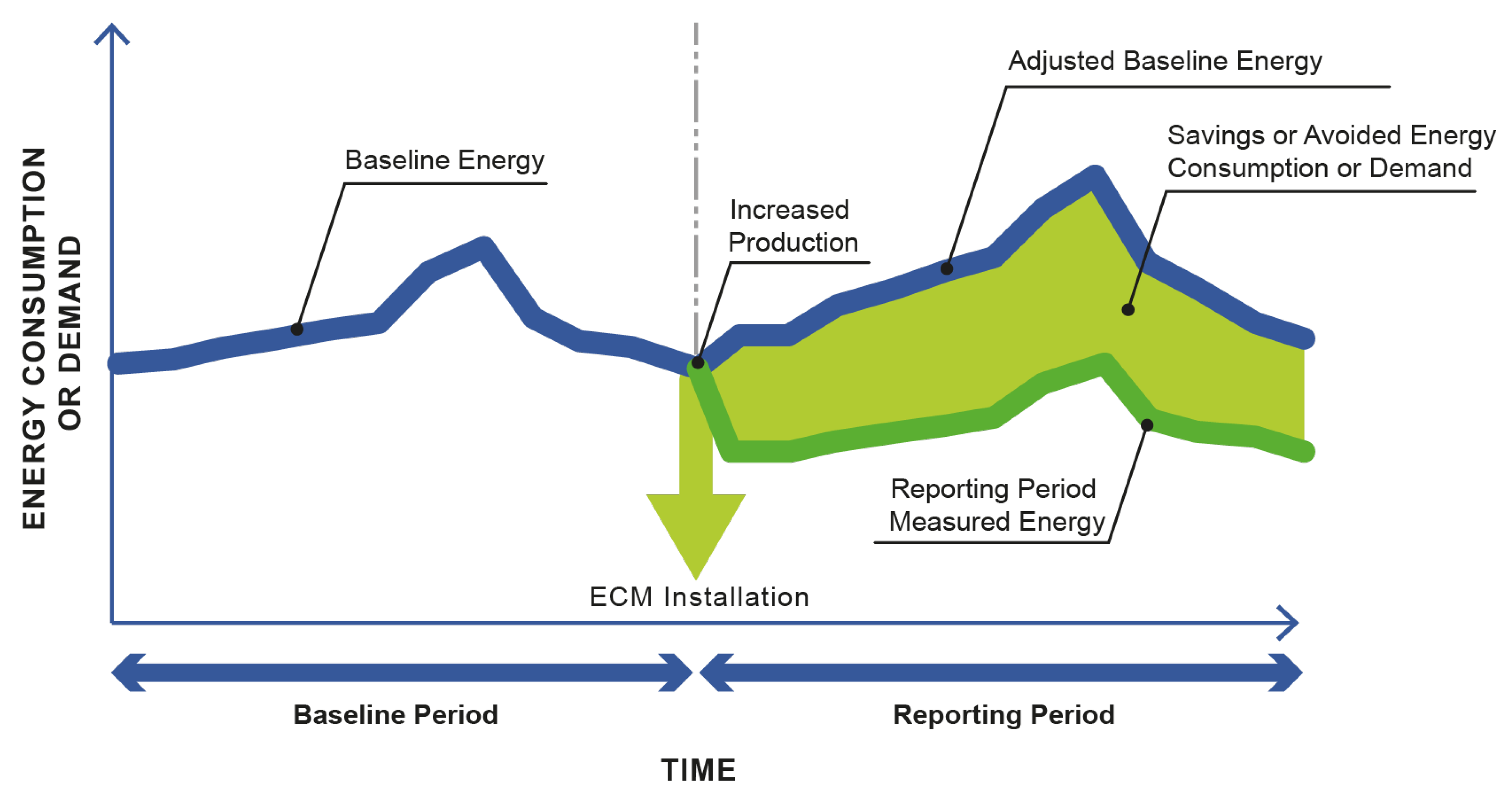
Figure 1 illustrates the measurement and verification procedure using long-term energy prediction models. A period of baseline energy consumption is used to create a machine learning prediction model to evaluate how much energy a building would use in a
status quo baseline mode. An energy conservation measure (ECM) is installed and the difference between the baseline is the avoided energy consumption or demand. This process is crucial for the implementation of energy savings implementations as it gives building owners, designers and contractors a means of evaluating the success of such measures.
1.1. Contemporary Building Energy Prediction
A recent comprehensive review of building performance prediction studies is available that describes the models, techniques, input features and uses for energy prediction in buildings [
10]. This study reviewed research that implemented the most common prediction modeling techniques as applied to building energy prediction. These models include Support Vector Machines (SVM), Artificial Neural Networks (ANN), Ensemble methods and various other techniques. A majority of the literature focuses on a single building or a small set of buildings case studies. Other ML reviews in the building industry show similar libraries of work [
11,
12].
The concern of the recent work in this area is the use of training data from a single case study building.
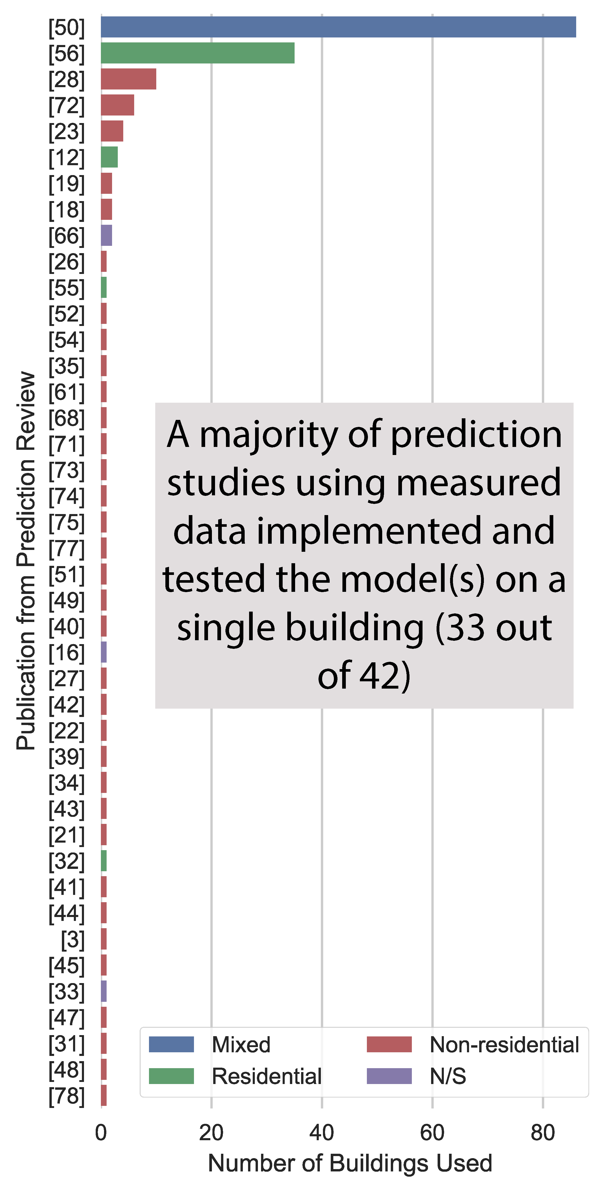
Figure 2 illustrates the number of buildings used to train models in a selection of long-term prediction papers from the previously-mentioned review publication [
10]. A majority of the models produced were implemented on only a single building. Case studies are an integral part of the building performance research community as they provide a tangible example of a new technology or method on a real building project. However, the challenge of using a case study as a machine learning application is that the results may not be generalizable across other types of buildings. Training a machine learning model on such a small set of data results in a solution that is designed specifically for that scenario. Such development produces models that have questionable value when applied to the broader building stock.
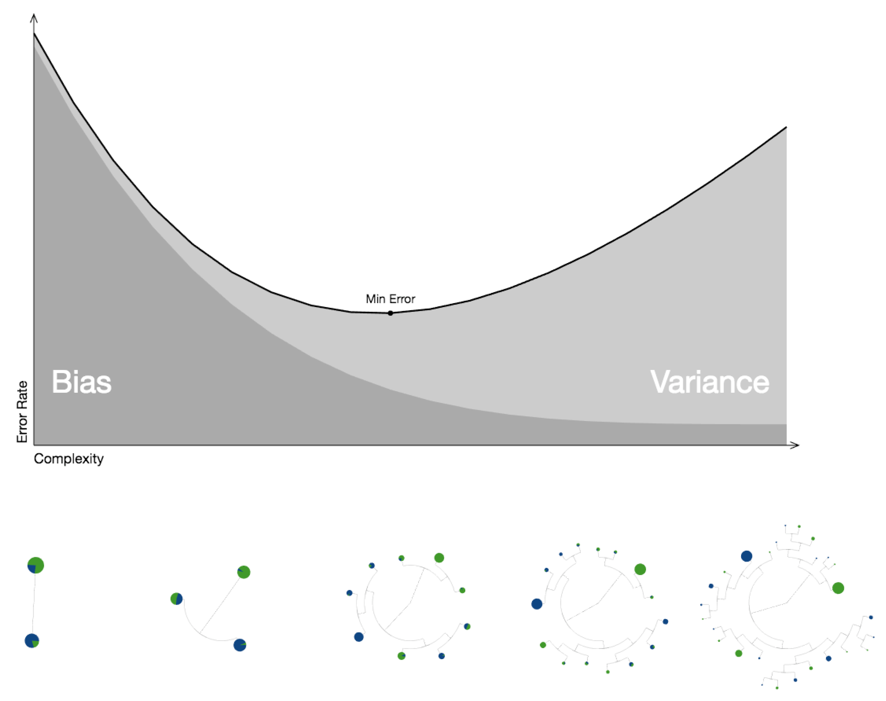
This type of generalizability challenge is discussed extensively in the machine learning community. This concept is related to the bias-variance trade-off that is illustrated in
Figure 3. A model with high bias suffers from a lack of complexity to capture the behavior that is occurring in reality in a meaningful way. This model would be considered as a scenario that is potentially
underfitting the data. On the other hand, an overly complex model suffers from high variance; this model can capture all the detailed behavior in the data that is used to train the model, but the model does not perform as well with new data sets (buildings) or future data.
Three fundamental studies were completed in the last four years, which took the process of machine learning for prediction to a diverse set of buildings. The first used 400 randomly selected buildings and applied six conventional, open prediction models to create a measurement and verification baseline [
8]. The next study used 537 buildings and applied ten prediction models to understand further which model performed best among a large set of building [
14]. The final study focused on the evaluation of what percentage of the building stock are appropriate to be used with
automated methods as developed in the previous two studies [
15].
Overall, these studies tested an extensive set energy prediction methods on a large set of buildings and this method was a step in the direction of generalizability of energy prediction models. However, these studies are problematic for use as a benchmarking data set for other researchers due to the lack of access to the exact models or data used. Access to these aspects of their studies would allow future techniques to be compared directly through the application of the old machine learning methods on new data or implementation of modern methods on their old data. These studies give the community an understanding of what models work better than others in the context of the bias-variance trade-off, but they do not provide the ability to test new models and techniques.
1.2. The Importance of Benchmarking
Despite the advancement of machine learning and prediction for performance data for buildings, a significant barrier to wide-spread dissemination is that the techniques are not easily reproducible and the results are not generalizable. Engineers, data scientists and researchers should be asking themselves does my machine learning technique scale across hundreds of buildings? And is it faster or more accurate? How do we compare, each technique against previously created methods?
The time-series data mining community identified this problem as early as 2003: “Much of this work has very little utility because the contribution made”…“offer an amount of improvement that would have been completely dwarfed by the variance that would have been observed by testing on many real-world data sets or the variance that would have been observed by changing minor (unstated) implementation details [
16]. This research group has most recently completed an extensive review of time-series classification algorithms on the UC Riverside open time-series data set [
17,
18].
Since then, a large portion of the machine learning community has created a program called
MLPerf that uses benchmark data sets to test the software, hardware and cloud-based solutions for applications such as image classification, speech recognition, sentiment analysis and several other common machine learning challenges (
https://mlperf.org/). This effort is predicted to move the entire community forward by allowing for quantitative comparison of the library of techniques in the community. Several other good examples of benchmarking data set and analysis can be found in specific scientific domains such as biology [
19], information retrieval [
20] and intrusion detection [
21].
The built environment still struggles with model generalizability despite these advancements in the larger ML community. Most of the existing building performance data science studies rely on each researcher creating their methods, finding a case study data set and determining efficacy on their own. Not surprisingly, most of those researchers find extraordinarily positive results. However, the ability to compare those results to other publications and techniques is limited.
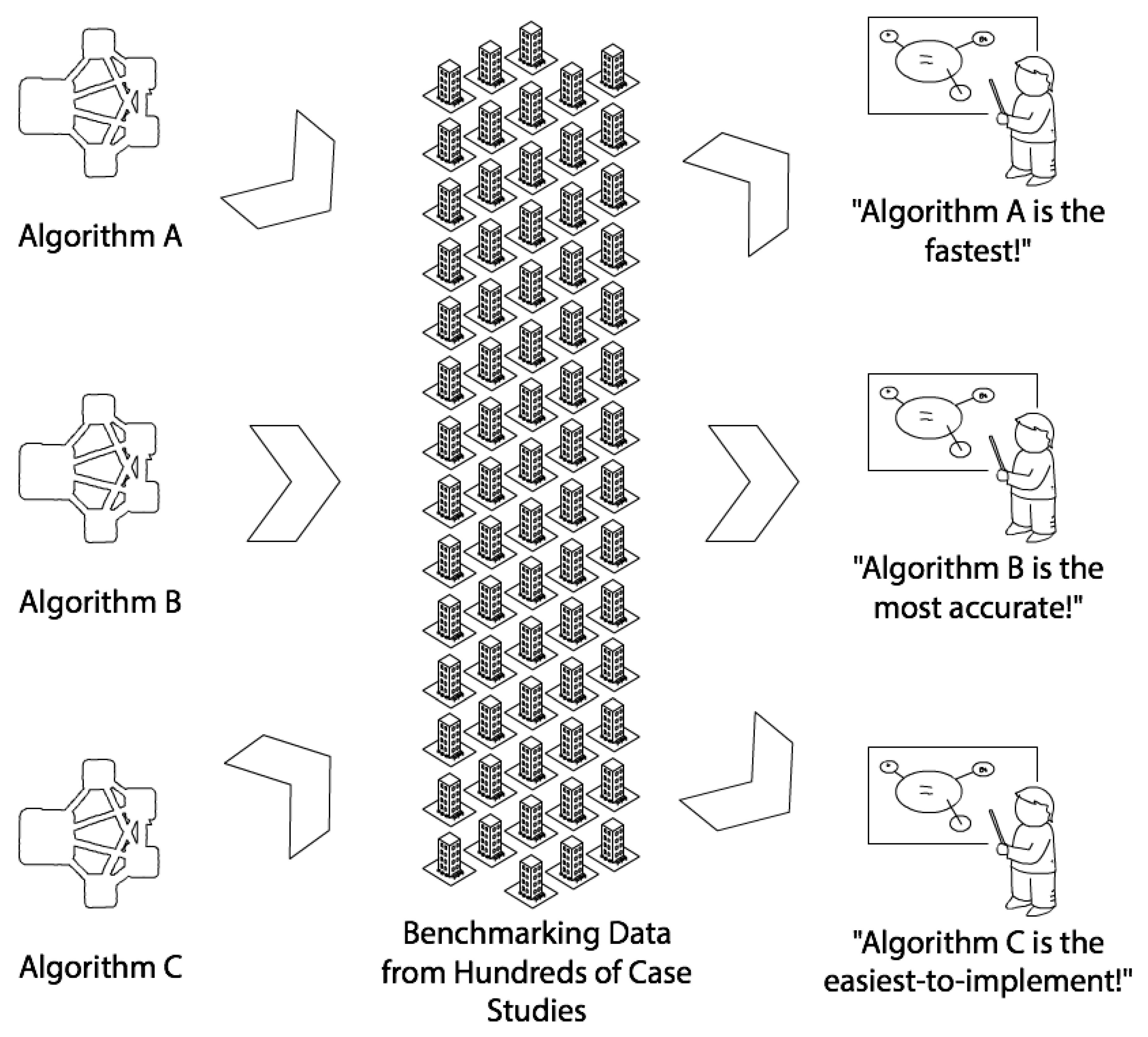
Using an extensive, consistent benchmark data set from hundreds (or thousands) of buildings, a researcher can determine how well their methods perform across a heterogeneous data set. If multiple researchers use the same data set, then there can be meaningful comparisons of accuracy, speed and ease-of-use.
Figure 4 illustrates the vision that benchmarking can achieve in this context. The purpose of this paper is to establish an example of machine learning benchmarking for energy forecasting and prediction.
The creation of benchmarking data sets and methods sets the research community towards an environment in which there is a measure of accountability in the claims made by new algorithms. These new techniques will likely be implemented on the test case(s) developed in the course of a research study but will also need to be applied as much as possible to benchmarking methods to show which type of improvement is occurring in the literature and the quantification of development.
Good Examples from the Past—ASHRAE Great Energy Predictor Shootout I and II
In the non-residential building research domain, there is a single set of examples of a benchmarking data set that was utilized for several machine learning studies. This set is the
Great Energy Predictor Shootout competitions held in the early 1990s and hosted by the ASHRAE Society. The first competition included the use of a single building’s electrical, cooling and heating meters in a contest where the participants were asked predict a single month of data using three months of training data [
22]. This competition resulted in several publications based on the top set of performers. A second competition was held, the aptly-named
Great Energy Predictor Shootout II that asked participants to predict the energy savings for an energy savings project [
23]. These data sets have since been used as a benchmarking comparison data set on several studies, including one focused on residential modeling using SVM [
24] and another that predicts consumption of office buildings in Greece [
25].
1.3. Improving Model Generalizability—Open Benchmarking Data Sets and Open Models
This paper outlines a demonstration of how benchmarking of performance prediction models can be accomplished on an open data set using open-source prediction techniques. The variability of accuracy results across different sizes of machine learning implementation strategies will be tested and discussed. Initially, in
Section 2, an overview of prediction considerations for building energy performance is reviewed. Next, in
Section 3, a framework for implementation is outlined using an open data set of 482 buildings. In
Section 4, the results are showcased and interpreted in the context of the different primary use types and operations considerations.
Section 5 describes the usefulness and interpretation of this test case scenario and potential future directions for the prediction model development community. Finally, in
Section 6, a discussion of the conclusions, limitations and a request for data inclusion from future researchers are presented.
2. Review of Building Energy Prediction Input Considerations
To initiate the prediction model discussion, an overview of the conventional energy performance prediction considerations is covered in this section. These aspects of machine learning-based modeling for buildings are most prominent in non-residential buildings such as offices, educational facilities, laboratories and health-care. These categories are the key considerations when developing prediction models for buildings.
2.1. Daily, Weekly and Seasonal Schedules
Buildings operate on several types of schedules. A majority of non-residential buildings have
occupied and
unoccupied periods that usually coincide with daytime and nighttime. These diurnal cycles are generally one of the best indicators of the building use type—that is, offices are open from 9 a.m. to 6 p.m. and hotels are most active from 6 p.m. to 10 a.m. An example of daily pattern extraction and analysis is found in the
DayFilter process [
26]. Most buildings also have a weekly schedule; the default being certain behavior on weekdays and different behavior on weekends. Finally, many buildings have seasonal changes such as when educational buildings have certain behavior during a regular session versus during breaks or holiday seasons. Extraction and analysis of longer-term schedules are covered extensively in an overview of temporal feature extraction from meter data using the STL package [
27,
28]. The concept of scheduling in non-residential buildings is most often related to the predefined schedules programmed into the automation systems in the building, unlike the human behavior that is discussed later. These schedules are determined usually by the operations and maintenance policy or by the energy management group within an organization. Many buildings have very predictable schedules, while others are much more volatile. Modeling such behavior can often be done using time-series methods that find auto-correlation behavior or by using date/time features as inputs to prediction models.
2.2. Human Behavior
The concept of
human behavior as an influence is similar to the previously-discussed schedules; however, there is a more stochastic element to this behavior. Buildings that are more influenced by occupant behavior generally have demand response-based control systems that use sensors, cameras or other detection methods to modulate systems only when humans are present or using the space for a specific purpose [
29]. Sometimes humans even can control spaces using various types of interfaces with the building, although this is less common in non-residential buildings. Modeling occupant behavior is considered more complex than schedule as human behavior can be less systematic; thus, auto correlation-based time-series methods are less effective.
2.3. Weather
A major energy-consuming component for most buildings is heating, ventilation and air-conditioning (HVAC) systems. Intuitively, these systems tend to use more energy as the outdoor conditions get hotter (in the case of cooling) or colder (in the case of heating). Often this relationship is linear, but it can also be non-linear based on the HVAC system type and operation policy. Two common building performance modeling techniques address the influence of weather using
change point models [
30] and the
time-of-week and temperature [
31]. The degree of influence of weather varies greatly among the building stock. It is influenced by the percentage of internal load versus envelope-based load, HVAC system type, climate and other factors.
2.4. Non-Routine Events
Non-routine events are disruptions in the regular operation of a building due to events such as a change in the operational schedule of the building, equipment breakdowns and events or human behavior that is highly irregular as compared to past behavior. These events could be planned or unplanned by the operations and facilities management staff. Non-routine events are hard to predict with conventional input variables but models can be tuned to quickly adapt to the change using approaches related to change-point prediction or other types of behavior change detection techniques. Changepoint detection models are often unsupervised and some techniques have been adapted from the analysis of social media data to be used on energy meter data [
27,
32].
3. Benchmarking Open Source Methods on Open Building Energy Data for Long-Term Prediction
The goal of this paper is to show an example benchmarking analysis applied to a diverse enough data set to illustrate the benefits of scalability and generalizability amongst the building stock. The regression testing framework for this paper is outlined in this section. The open hourly data from the
Building Data Genome Project (BDG) is used in this paper as a starting point [
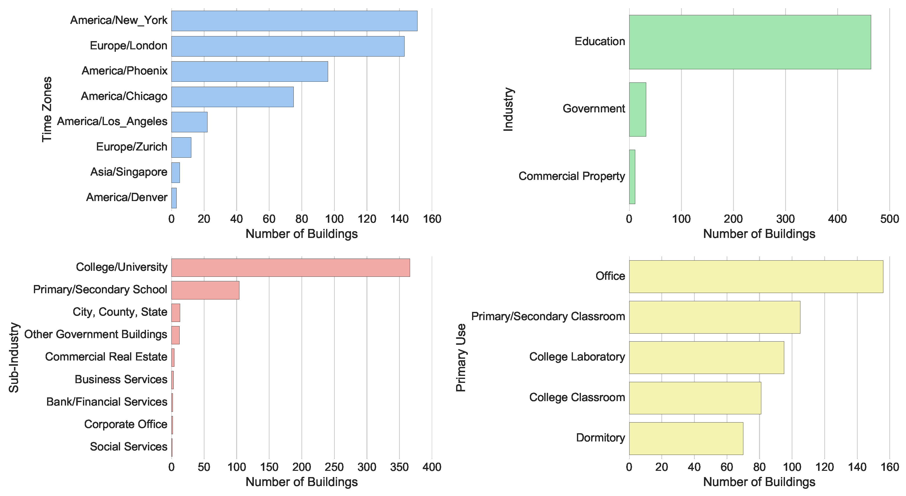
33]. This data set includes data from over 500 buildings, mostly from educational institutions.
Figure 5 illustrates the breakdown of four meta-data points from this data-set.
3.1. Machine Learning Input Variables
One year of whole building hourly electrical meter data is used in this process from a subset of 482 buildings from the main BDG repository. These buildings were selected due to the temporal and metadata completeness. Various temporal and meta-data based model input variables were extracted from the raw data for use in the machine learning process. The input variables available as predictors of energy consumption are outlined in this section.
Table 1 outlines the basic set of machine learning input variables used in this benchmarking approach. The overall goal of this benchmarking process is to predict the hourly whole building electrical meter data consumption of each building using these input variables.
3.2. Training and Test Data Set Scenario
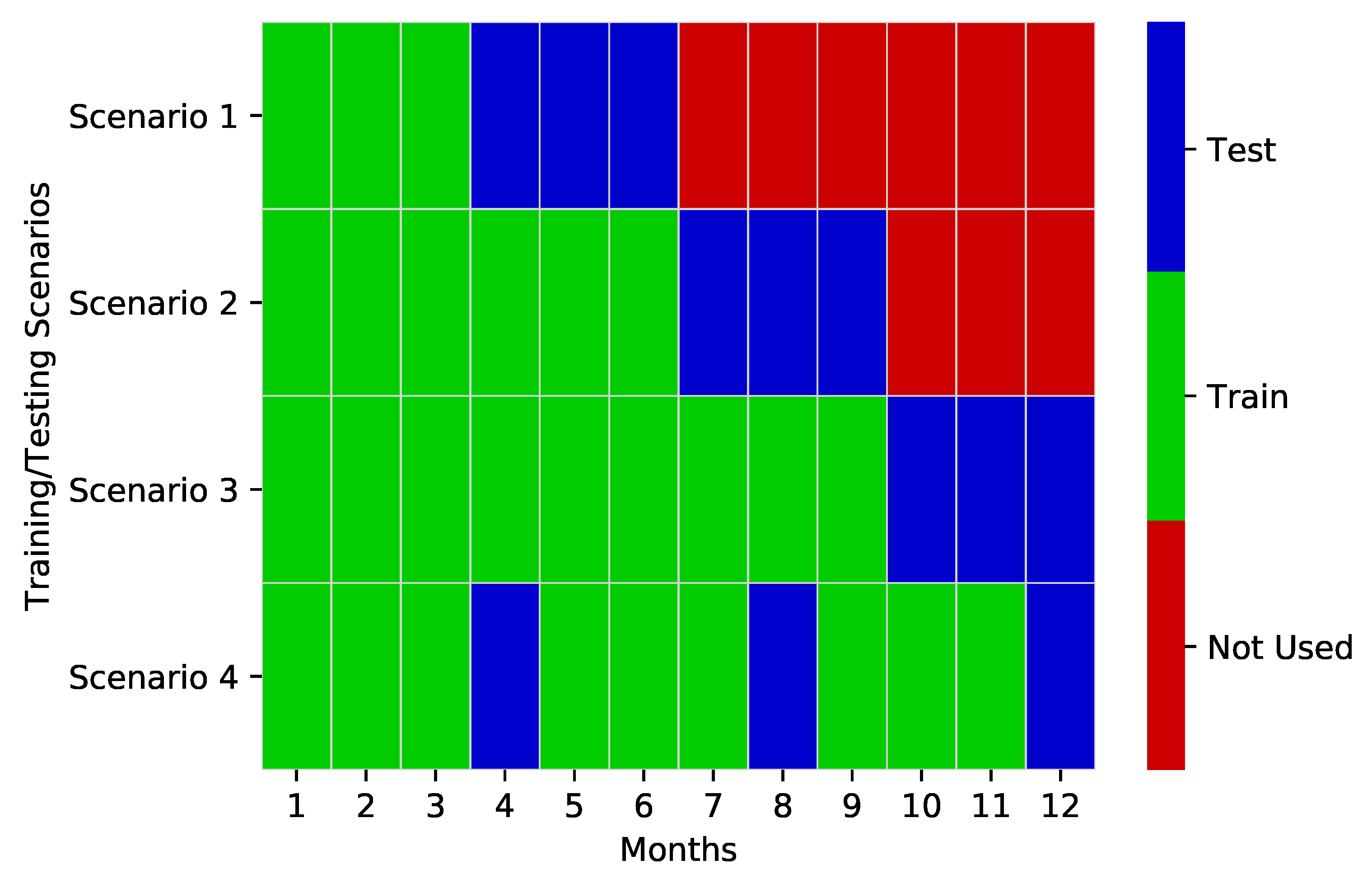
For the comparison of various open-source techniques, a simplified training and testing scenario is utilized for the comparison. Four different training and testing data scenarios are tested, as seen in
Figure 6. Scenarios 1–3 are made up of 3, 6 and nine-month training windows and a three-month continuous testing window. Scenario 4 is made up of 3-month training windows followed by a one-month test window that repeats itself three times. These scenarios provide a certain level of cross-validation that is realistic in the context of medium to long-term energy prediction in the built environment.
3.3. Open Source Regression Models from Sci-Kit Learn Python Library
The regression model catalog from the Sci-kit Learn Library is used in this benchmarking process [
34]. We use these models as a starting point for the benchmarking process as many of these models have been developed for decades and are some of the most often used prediction models in the machine learning community. The more extensive array of more advanced models (e.g., deep learning, specific energy-focused prediction models) is left outside the scope of this paper as these will be the
improved techniques that the broader research community would likely be testing. The models from this library use used with default hyperparameter and attributes settings.
This study focuses on general forecasting methods as a foundation for comparison for more building domain-specific regression or prediction models. These models do not take into consideration the auto-correlation aspect of prediction or the building context-specific nature of the built environment.
3.4. Accuracy Metrics
The two metrics used in this analysis to evaluate model fit are the Coefficient of Variation of the Room Mean Square Error (CVRMSE) and the Mean Absolute Percentage Error (MAPE). MAPE is a commonly used loss function for regression problems and model evaluation. CVRMSE is one of the metrics most commonly used in performance analysis of energy models in the building industry [
9,
35]. The metrics are a combination of the values of number of compared values (
n), measured values (
m), predicted values (
f) and parameters (
p).
Table 2 illustrates the formulas for these metrics. ASHRAE Standard 14 guides the use of CVRSME for building performance comparison and fixes the
p value at 1.
4. Results
The range of regression models was implemented on the 482 buildings from the Building Data Genome Project and two types of analysis are illustrated in this section. The first is focused on the distribution of model fit across the population of buildings for each of the models. The second analysis chooses the model with the highest overall accuracy across the building set and shows the diversity of results across different randomly chosen sizes of prediction model implementation cohorts to illustrate the generalizability of the tested models.
4.1. Model Fit Overview for the Example Benchmarking Scenario
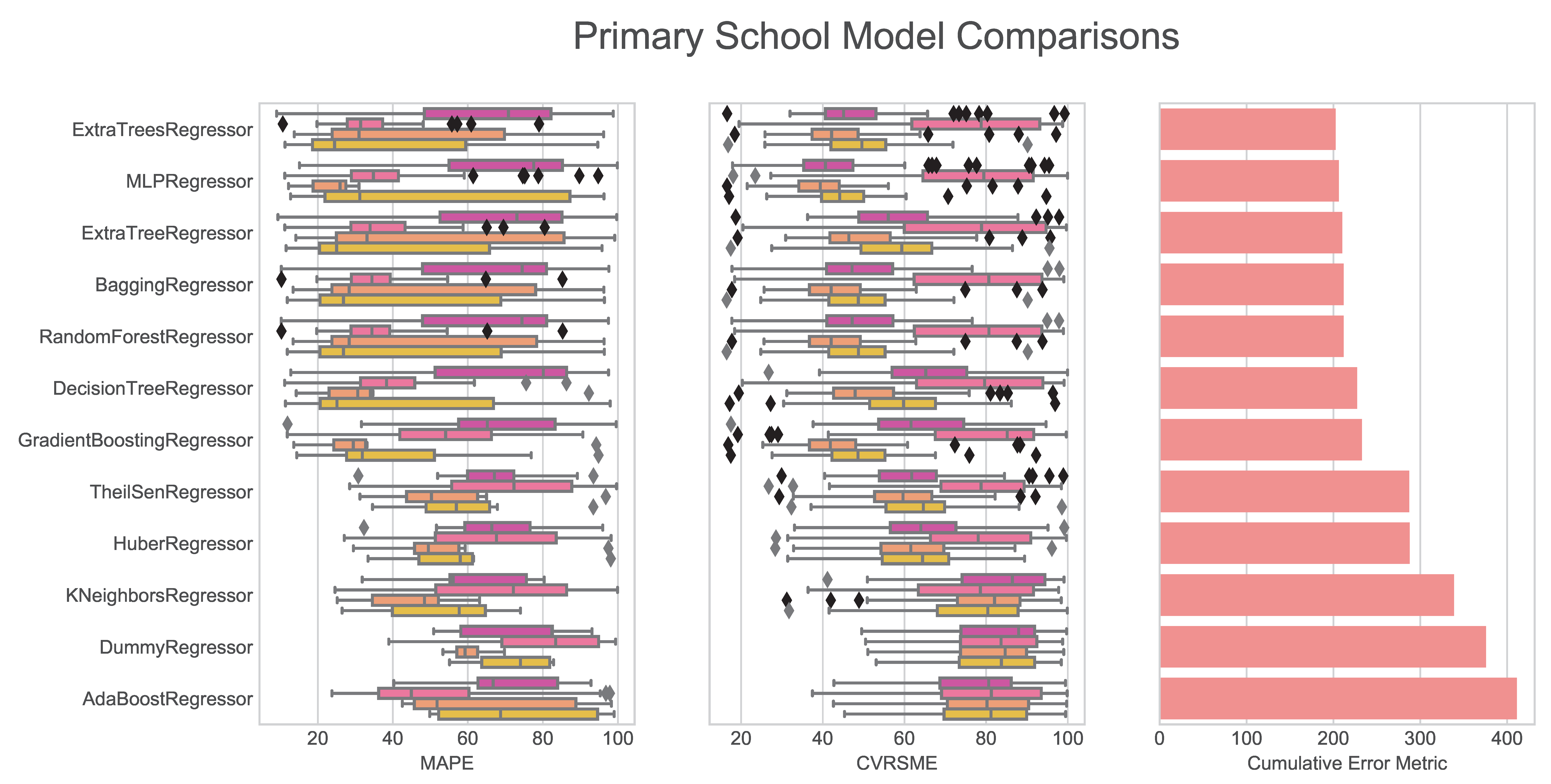
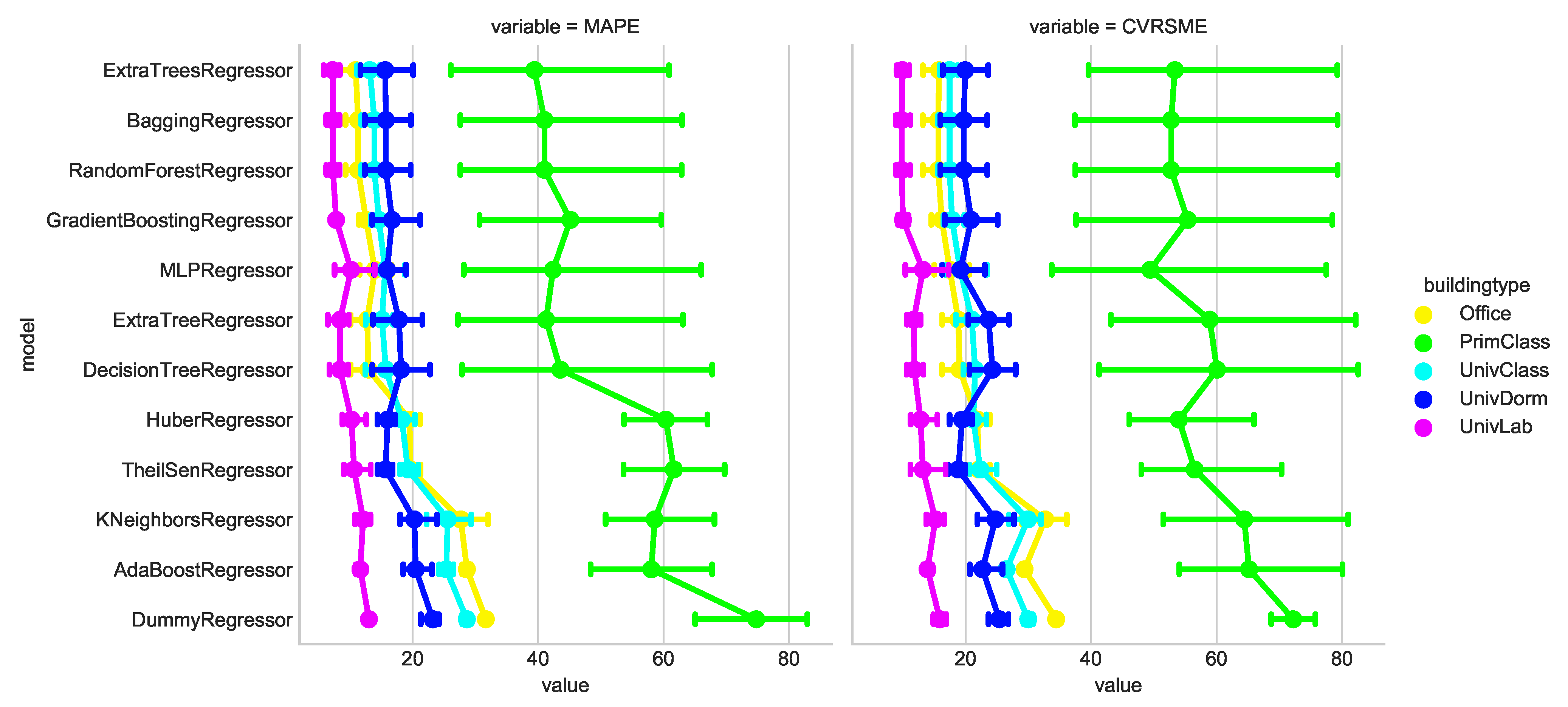
Figure 7 illustrates the twelve Sci-Kit learn models applied to all the building use types using the MAPE and CVRMSE metrics. The detailed results of all model implementations can be found in
Appendix A. The graphics in the appendix provide a more detailed breakdown of each of the building use types according to all three error metrics as well as an analysis of each of the four training/testing scenarios. This analysis is provided as an example of a typical predictive model implementation scenario. Future researchers can take this analysis as a template to test their prediction models across the range of buildings.
For the example analysis, it appears that laboratories have the highest accuracy across all of the models. This situation could be due to laboratories being the most systematically schedule-driven of all the building types. Laboratories often have large equipment that is operated continuously or in set time schedules throughout an entire year. University classrooms and offices behave in similar ways across the models as these two use types are often identical and many of these buildings are mixed-use types. University dormitories have the fourth-highest accuracy for most of the models; however, they are better fits for models such as the Huber Regressor or the TheilSen Regressor. Finally, the Primary School buildings are by far the worst performers among the building use types. These buildings are dependent more on human behavior within their annual schedule phases, resulting in the lack of predictability using the methods and models outlined in this simple example.
This analysis shows that the models tested have a range of behavior and there is some consistency of which models perform better or worse. The primary school classrooms pose a very distinct challenge as opposed the other building use types. This scenario shows that a much more complex model is likely necessary to model that particular building use type adequately. There would probably need to be an ensemble or series of prediction models developed and tested to implement on the whole data set to show overall improvement. These schools, in particular probably need additional input data as well to be more adequately modeled.
4.2. Generalizability Analysis
In this analysis, the diversity of modeling accuracy is put in the context of different sizes of prediction model implementation populations. The goal of this analysis is to show that for each machine learning modeling approach the
usefulness of the modeling technique is better proven with the larger the size and diversity of implementation on real-world building data sets. The first way to illustrate this concept is to show the range of modeling accuracy for our simple benchmarking example across all the buildings tested.
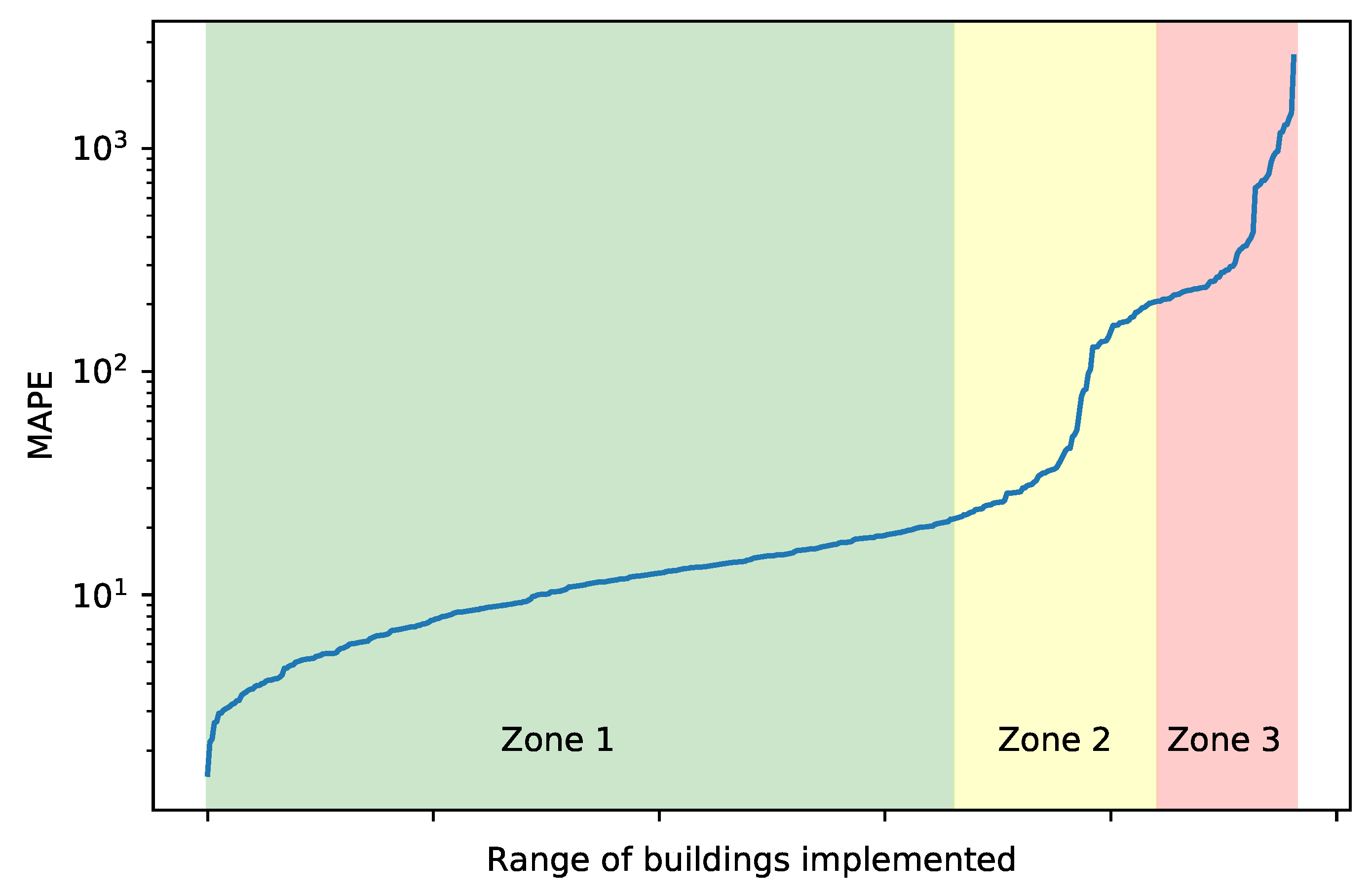
Figure 8 illustrates a line chart that plots the increasing error rates across the 482 buildings using the
ExtraTreesRegressor model, which was the best performing model for most of the building types. This visualization has been manually segmented into three zones. Zone 1 illustrates buildings (almost two-thirds of the data set) in which the example benchmarking modeling scenario presented in this paper is considered adequate or
good. It can safely be stated that this model is generalizable across that cohort of buildings. On the other hand, Zones 2 and 3 illustrate buildings in which either the input features or the model itself cannot account for behavior in those buildings; thus they do a
poor or very poor job at predicting their consumption. Most of these buildings are from the previously-mentioned Primary/Secondary School use type. Future researchers would add complexity to the overall modeling strategy or invent a whole new approach to create a paradigm in which the entire range of buildings shows
good performance.
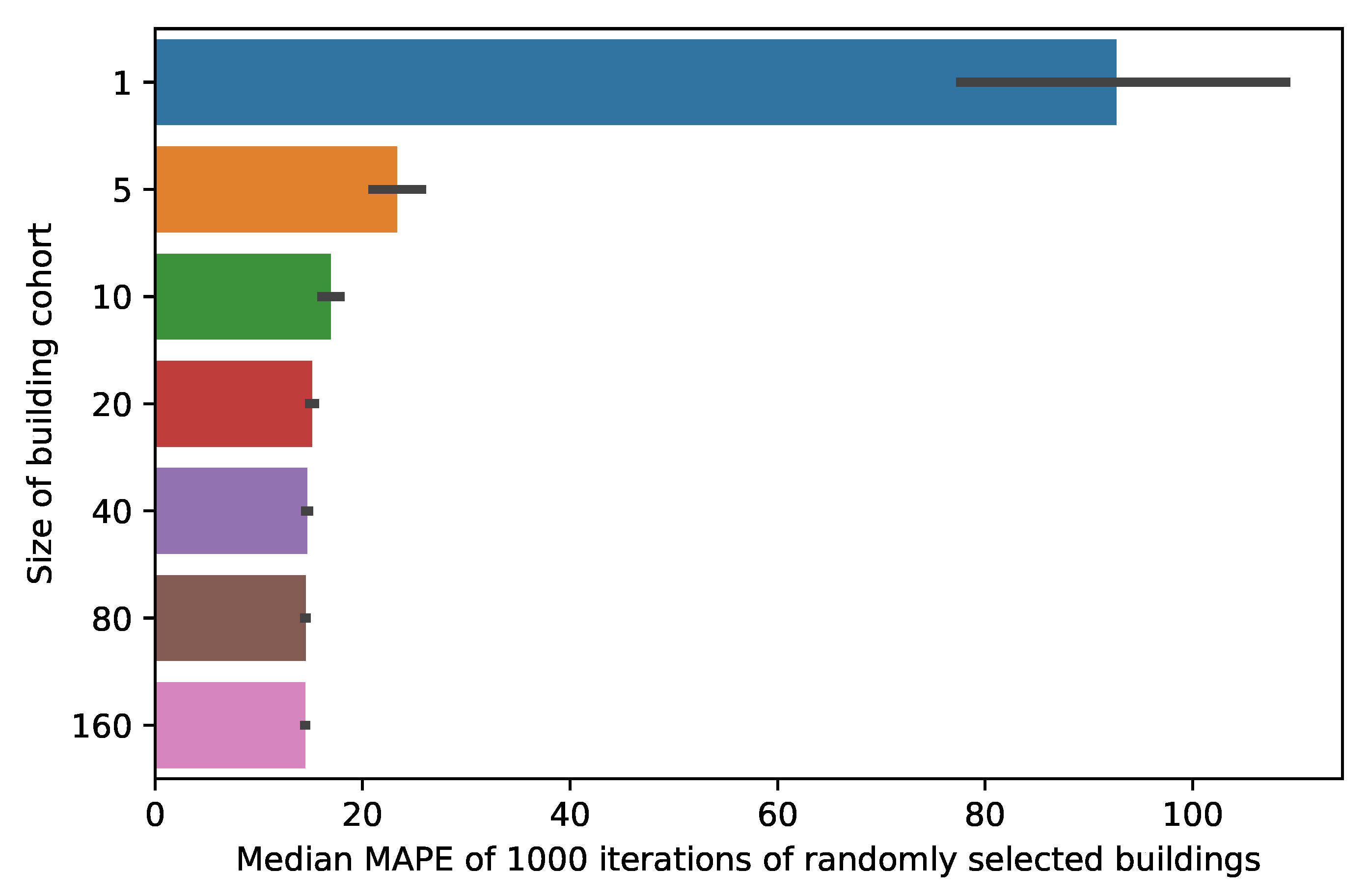
To further investigate, different cohorts (or groups of buildings) are randomly extracted from the performance accuracy data set to show the median MAPE values based on how many buildings are in the cohort. In
Figure 9, the MAPE from various sizes of prediction model implementation were extracted from the overall data set. One thousand random extractions of each of the cohort sizes yielded are plotted as the average median accuracy with uncertainty bars. In this scenario, a single, randomly selected building would have a much higher median error rate than even a group of five buildings. Median was chosen as the metric as it reduces the influence of the extreme outliers of error. As more buildings are added to the analysis, the error rate gets closer to the actual
generalizable error rate for this particular modeling technique, in this case, a MAPE of around 14%.
This example scenario illustrates that using a randomly selected building to apply a simple baseline model produces worse results than for a more extensive set of buildings. However, in a typical predictive model case study situation, an analyst often picks a building and builds a more complex model specifically for that building. In that situation, the analyst chooses specific input features from that building that would result in the lowest error. This model, while accurate on that single building, would likely be less reliable on the more substantial portfolio of buildings. This case would cause the error rate for the single building cohort to be much lower than the larger groups. This scenario is not tested in this paper due to the constraints of building and testing much more complex prediction models.
It should be noted that the analysis in this section should only be interpreted in the context of the buildings, input features, models and model fit metrics outlined in this paper. This whole scenario is provided as a template for future researchers and companies who want to implement various modeling techniques on the BDG data set while adding their own case study data sets. The subsequent sections outline some areas of potential future improvement in this pursuit.
5. Discussion
5.1. Long-Term versus Short-Term Forecasting Applications
It should be noted that this benchmarking test setup is aligned with the use of prediction in the context of measurement and verification. This type of prediction is considered medium or long-term forecasting focused on the evaluation of energy savings of building performance interventions. This application has several characteristics that differentiate it from short-term applications such as day-ahead prediction for control and demand response. For example, long-term forecasting is usually retroactive as the energy savings prediction is focused on what energy the building would have consumed if the intervention had not taken place. This situation means that input variables such as weather are known and not forecasts themselves. Additionally, in this benchmark scenario, only a few time-series features are used, notably the time-of-day and day-of-week. Short-term forecasting usually incorporates more of the near-term historical structure of the data to make forecasts. The relevance of what happened yesterday or the day before can be informative to the short-term application. The benchmarking process in this paper could be adapted to focus on these short-term forecasting applications.
5.2. On the Need for Generalizability of Building Performance Forecasting in Various Applications
The results of this analysis illustrate that a narrow set of modeling configurations produce different accuracy results across a range of buildings. If the goal of a machine learning expert is to create accurate models for the whole population of buildings, then there is a significant amount of effort to be done to improve the generalizable accuracy of the model strategy. The need for such generalizable modeling strategies is emerging as the size of internet-of-things (IoT) and energy metering grows exponentially. Portfolio managers might have hundreds of buildings with each building having numerous sub-metering systems at the different levels of the energy-consuming hierarchy. It is possible to develop and manually tune a machine learning model for a few meters but impractical for hundreds or thousands of data streams.
However, in current practice, it is not always the objective to scale a model across numerous buildings. The machine learning expert is instead tasked with the development of a data-driven model for a single building for scenarios such as demand response and automated fault detection and diagnostics. In these scenarios, the impact of the customized models is more valuable that the scalability or generalizability and there are resources and human resources to build customized models. The primary reason for the lack of generalizability of techniques in the literature is likely due to the contemporary lack of focus on the objective of individual model accuracy rather than overall scalability amongst large numbers of buildings.
5.3. Potential Future Enhancements of the Benchmarking Process
As previously discussed, this benchmarking implementation is limited in its application of prediction models, feature extraction techniques and parameter tuning. This subsection discusses the potential future advancements in modeling frameworks in the context of the benchmarking example in this paper and relevant recent prediction studies.
5.3.1. Testing Model Hyperparameters in the Benchmarking Process
Machine learning models often have several inputs that specify thresholds and options that influence the way the model trains or predicts using the input training data and features. These hyperparameters must be preset before implementation as they have an impact performance. For example, neural network models such as multi-layer perceptrons have input parameters related to hidden layer attributes and iterations that enable a user to tune them for best performance on a particular data set. Further benchmarking work could focus on these modeling aspect to test which configuration of parameters results in the best model fit.
5.3.2. Using More Advanced Time-Series Prediction Techniques
There is a library of time-series specific modeling techniques that could be tested on the benchmark data set to understand how the univariate temporal structure of each meter could be used for prediction. A recent review covered the used of more advanced time-series techniques for building energy prediction [
36]. This review illustrates the accuracy of the six most popular models: ANN [
37], ARIMA [
38], SVM [
39], Fuzzy [
40], Grey [
41] and MA and ES [
42]. All of these top-performing time-series models achieved less than 3% MAPE, yet only on a single or small set of meter data streams. Once again, in the overall review, only a few studies used more than one building to train and test their technique or released the data for others to implement and compare their techniques. These techniques are valuable but the community deserves to understand how generalizable these techniques are and how they scale.
5.3.3. Transfer Learning: Using Training Data from the Whole Population for Prediction of Each Building
This area of innovation in modeling would seek to create prediction models that use the data from hundreds or thousands of buildings to predict consumption for a single building. These models would try to predict which other buildings are so similar due to their metadata or behavior that they could be used to enhance model training. An analogous scenario in building prediction is the use of surrogate models derived from physics-based simulation [
43]. Another example is an application that focuses on using cross-building transfer learning to model smart meter data in scenarios where unlabeled data exists [
44].
5.3.4. Automated Feature Extraction and Deep Learning Methods
In the example scenario from this paper, input features for prediction were extracted in a somewhat manual process using engineering and professional judgment about which behavior needed to be captured to predict the hourly energy consumption. This approach works for many buildings but often there are complicated situations that manual feature engineering will miss. New types of modeling, such as deep learning model can capture a more significant amount of more complex behavior without manual feature engineering. These models have shown tremendous value in image and video recognition applications and have been applied to building performance prediction several times [
45,
46,
47]. These studies show promise but once again, are applied to a limited number of buildings or sets of buildings. The community would benefit in understanding whether the complexity and lack of interpretability of these models are worth the potential increase in accuracy across several building types.
5.3.5. Finding Additional Phenomena to Measure or Collect that Can Be Used as Input for the Modeling Process
This scenario presented included a list of input features shown in
Table 1. These are commonly accessible input features for performance prediction and they capture consumption behavior for a majority of the buildings. However, numerous other phenomena could be digitized using sensors or harvested from data sources such as building information models (BIM). For example, carbon dioxide sensor data from the building management system (BMS) would likely enhance the ability to predict behavior related to occupancy. An explosion of internet-of-things (IoT) data is becoming available to use to supplement prediction models. However, the limitation of using these data streams is that all buildings in a benchmarking scenario would need to include such data for comparison to occur. Collection and processing of such data are not trivial.
5.3.6. Focus on the Accuracy of a Modeling Framework Rather Than an Individual Model
The reality of applying machine learning models to a large number of buildings is that techniques that generalize well will likely be a series of models and modeling and pre/post-processing steps. The literature usually categorizes these processes as
hybrids. This type of approach usually requires the sharing of code to be able to reproduce the results. Kaggle machine learning competitions are an excellent example of where elaborate ensembles and a whole series of modeling choices are what yields the best results, not any single model algorithm [
48,
49].
5.3.7. Integration of Data-Driven Modeling with Physics-Based White-Box Modeling
A significant opportunity exists to combine the decades of physics-based modeling in the built environment with machine learning models. The thermodynamic and heat transfer characteristics contained in those simulation input files could enhance with prediction capability of data-driven methods. The field of Bayesian calibration of simulation models provides the foundation for this effort [
50].
6. Conclusions
This publication gives readers a simple example of mainstream prediction techniques applied to a large, diverse data set. Five different primary use types of buildings were analyzed—offices, laboratories, university classrooms, dormitories and primary/secondary schools. The mainstream models and input variables in this process produced reasonable results for most buildings with ensemble methods such as decision-tree based techniques such as ExtraTrees and Bagging regressors. Primary/Secondary schools stood apart as a difficult building type to predict due to seasonal shifts. While these results are interesting, they are only relevant to the range of behavior from the 482 buildings tested. This publication intends to provide an example of the application of open prediction models to open data sets.
The results illustrate the there are a wide diversity of behavior types in the building stock and no single modeling technique can claim, so far, that it comprehensively accounts for all the different types of buildings or behaviors. Thus, the future of building performance prediction is likely to be dominated by modeling frameworks or ensembles of methods that can account for a broad diversity of behavior. Modeling techniques will likely filter buildings into groups that respond best to certain types of prediction models. With a growing benchmarking data set that encompasses more and more building types and behavior from the overall populations of buildings, the value of these more complex processes of models will be easier to showcase.
6.1. Limitations
The key limitation of this analysis is congruent with the limitation of machine learning in general: the models developed and the resulting metrics are limited by the range of training data utilized to build the models. The conclusions of the model comparison in this paper are only relevant to office, laboratories, classrooms and dormitories from university campuses in the context of the geographical and operational environments of the Building Data Genome Project data set. Thus, the primary goal of this analysis is not to be comprehensive in capturing the behavior of the building stock but to provide an example and data set that can be built upon with a more diverse set of data. It is crucial that additional data from thousands (or millions) of other buildings are added overtime for the methodology to achieve the main goal of a comprehensive benchmarking process. New algorithms coming into the public domain should be tested against this growing set of building data sets to quantify what improvements are being made in the domain.
Author Contributions
Conceptualization, methodology, investigation, writing and funding acquisition, C.M.
Funding
This research was funded by the Singapore Ministry of Education (MOE) grant number R296000181133.
Acknowledgments
Benchmarking of building performance prediction models is only possible through the donation of example data sets. The numerous public and anonymous data donors in the Building Data Genome Project made this publication possible.
Conflicts of Interest
The funders had no role in the design of the study; in the collection, analyses, or interpretation of data; in the writing of the manuscript, or in the decision to publish the results.
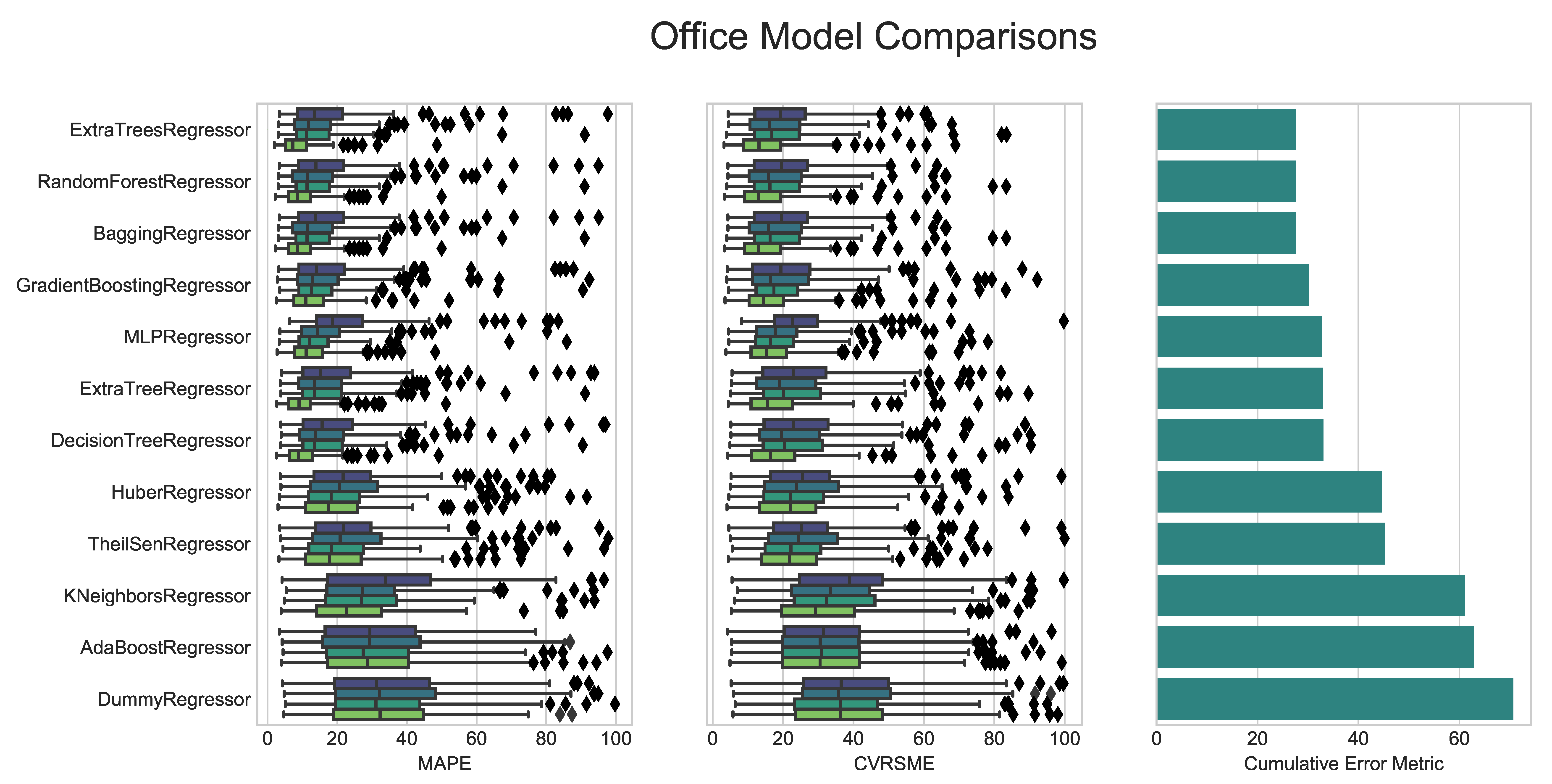
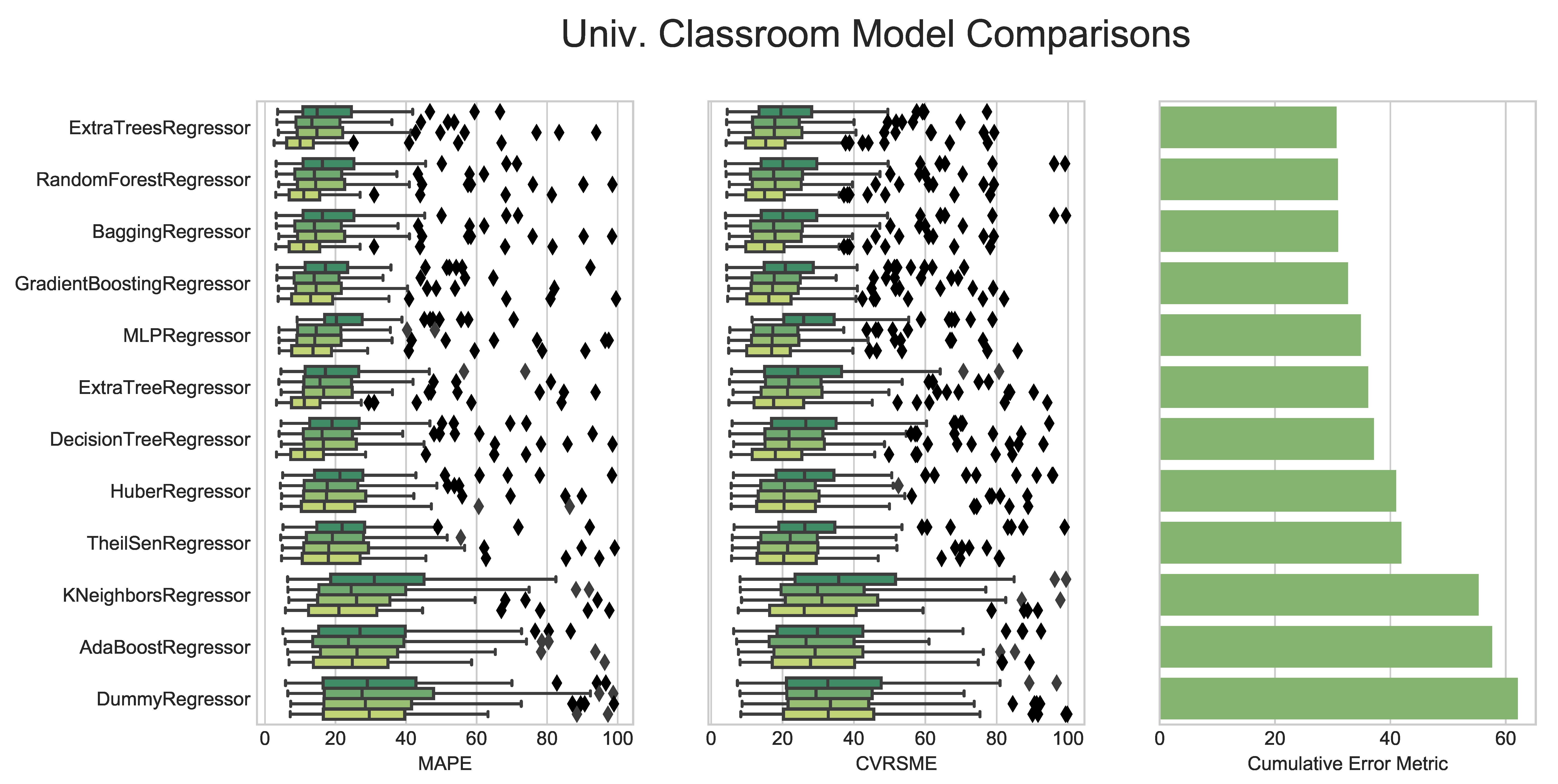
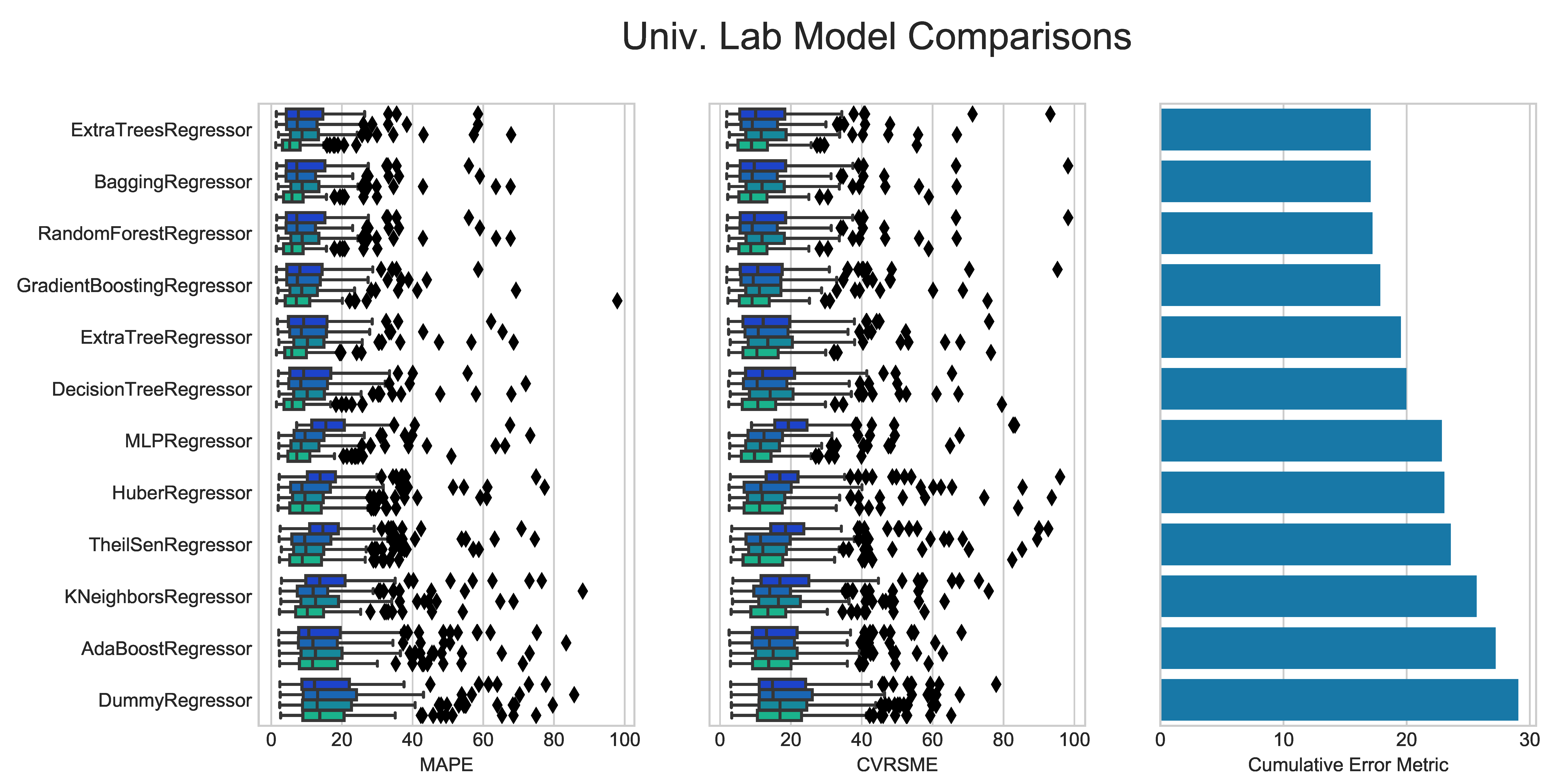
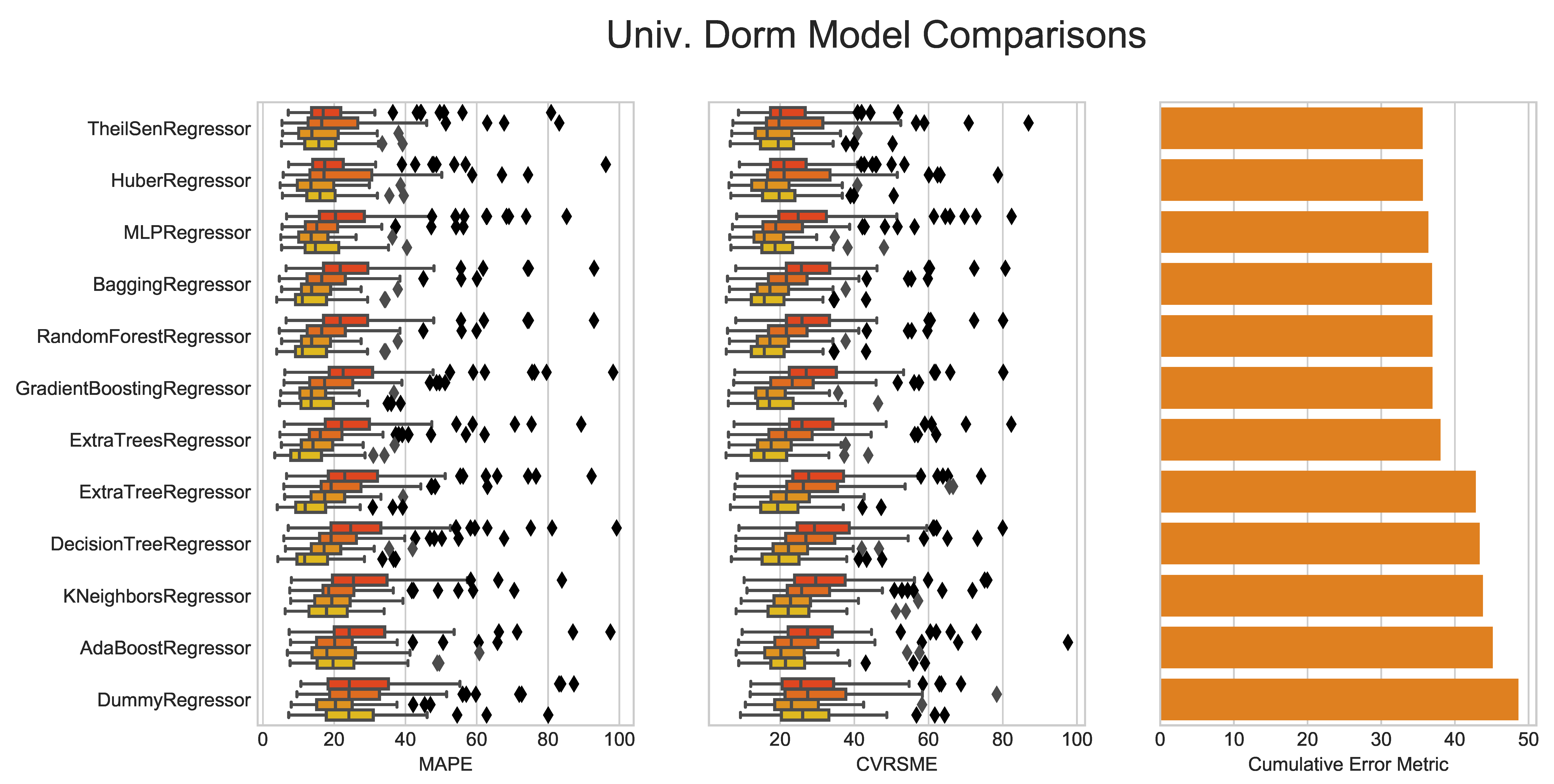
Appendix A. Detailed Model Comparison Breakdowns
Figure A1.
Detailed Breakdown of Benchmarking Models on Office Buildings.
Figure A1.
Detailed Breakdown of Benchmarking Models on Office Buildings.
Figure A2.
Detailed Breakdown of Benchmarking Models on University Classroom Buildings.
Figure A2.
Detailed Breakdown of Benchmarking Models on University Classroom Buildings.
Figure A3.
Detailed Breakdown of Benchmarking Models on University Laboratory Buildings.
Figure A3.
Detailed Breakdown of Benchmarking Models on University Laboratory Buildings.
Figure A4.
Detailed Breakdown of Benchmarking Models on University Dormitory Buildings.
Figure A4.
Detailed Breakdown of Benchmarking Models on University Dormitory Buildings.
Figure A5.
Detailed Breakdown of Benchmarking Models on Primary School Buildings.
Figure A5.
Detailed Breakdown of Benchmarking Models on Primary School Buildings.
References
- Agrawal, A.; Gans, J.; Goldfarb, A. Prediction Machines: The Simple Economics of Artificial Intelligence; Harvard Business Press: Brighton, MA, USA, 2018. [Google Scholar]
- Solomon, D.M.; Winter, R.L.; Boulanger, A.G.; Anderson, R.N.; Wu, L.L. Forecasting Energy Demand in Large Commercial Buildings Using Support Vector Machine Regression; Tech. Rep. CUCS-040-11; Department of Computer Science, Columbia University: New York, NY, USA, 2011. [Google Scholar]
- Fan, C.; Xiao, F.; Wang, S. Development of prediction models for next-day building energy consumption and peak power demand using data mining techniques. Appl. Energy 2014, 127, 1–10. [Google Scholar] [CrossRef]
- Borges, C.E.; Penya, Y.K.; Ferńandez, I.; Prieto, J.; Bretos, O. Assessing tolerance-based robust short-term load forecasting in buildings. Energies 2013, 6, 2110–2129. [Google Scholar] [CrossRef]
- Escrivá-Escrivá, G.; Álvarez-Bel, C.; Roldán-Blay, C.; Alcázar-Ortega, M. New artificial neural network prediction method for electrical consumption forecasting based on building end-uses. Energy Build. 2011, 43, 3112–3119. [Google Scholar] [CrossRef]
- Jetcheva, J.G.; Majidpour, M.; Chen, W.P. Neural network model ensembles for building-level electricity load forecasts. Energy Build. 2014, 84, 214–223. [Google Scholar] [CrossRef]
- Jain, R.K.; Smith, K.M.; Culligan, P.J.; Taylor, J.E. Forecasting energy consumption of multi-family residential buildings using support vector regression: Investigating the impact of temporal and spatial monitoring granularity on performance accuracy. Appl. Energy 2014, 123, 168–178. [Google Scholar] [CrossRef]
- Granderson, J.; Price, P.N.; Jump, D.; Addy, N.; Sohn, M.D. Automated measurement and verification: Performance of public domain whole-building electric baseline models. Appl. Energy 2015, 144, 106–113. [Google Scholar] [CrossRef]
- Efficiency Valuation Organisation. International Performance Measurement and Verification Protocol. Available online: http://www.eeperformance.org/uploads/8/6/5/0/8650231/ipmvp_volume_i__2012.pdf (accessed on 27 August 2019).
- Amasyali, K.; El-Gohary, N.M. A review of data-driven building energy consumption prediction studies. Renew. Sustain. Energy Rev. 2018, 81, 1192–1205. [Google Scholar] [CrossRef]
- Foucquier, A.; Robert, S.; Suard, F.; Stéphan, L.; Jay, A. State of the art in building modelling and energy performances prediction: A review. Renew. Sustain. Energy Rev. 2013, 23, 272–288. [Google Scholar] [CrossRef]
- Massana, J.; Pous, C.; Melendez, J.; Colomer, J. Short-term load forecasting in a non-residential building contrasting models and attributes. Energy Build. 2015, 92, 322–330. [Google Scholar] [CrossRef]
- Stephanie, T.C.Y. Model Tuning and the Bias-Variance Tradeoff. 2019. Available online: http://www.r2d3.us/visual-intro-to-machine-learning-part-2/ (accessed on 29 November 2018).
- Granderson, J.; Touzani, S.; Custodio, C.; Sohn, M.D.; Jump, D.; Fernandes, S. Accuracy of automated measurement and verification (M&V) techniques for energy savings in commercial buildings. Appl. Energy 2016, 173, 296–308. [Google Scholar] [CrossRef]
- Grandersona, J.; Touzani, S.; Fernandes, S.; Taylor, C. Application of automated measurement and verification to utility energy efficiency program data. Energy Build. 2017, 142, 191–199. [Google Scholar] [CrossRef]
- Keogh, E.; Kasetty, S. On the Need for Time Series Data Mining Benchmarks: A Survey and Empirical Demonstration. Data Min. Knowl. Discov. 2003, 7, 349–371. [Google Scholar] [CrossRef]
- Bagnall, A.; Lines, J.; Bostrom, A.; Large, J.; Keogh, E. The great time series classification bake off: A review and experimental evaluation of recent algorithmic advances. Data Min. Knowl. Discov. 2017, 31, 606–660. [Google Scholar] [CrossRef] [PubMed]
- Chen, Y.; Keogh, E.; Hu, B.; Begum, N.; Bagnall, A.; Mueen, A.; Batista, G. The UCR Time Series Classification Archive 2015. Available online: https://www.cs.ucr.edu/~eamonn/time_series_data/2015 (accessed on 27 August 2019).
- Sonego, P.; Pacurar, M.; Dhir, S.; Kertész-Farkas, A.; Kocsor, A.; Gáspári, Z.; Leunissen, J.A.; Pongor, S. A protein classification benchmark collection for machine learning. Nucleic Acids Res. 2007, 35, 232–236. [Google Scholar] [CrossRef] [PubMed]
- Liu, T.y.; Xu, J.; Qin, T.; Xiong, W.; Li, H. LETOR: Benchmark Dataset for Research on Learning to Rank for Information Retrieval. In Proceedings of the SIGIR 2007 Workshop Learning to Rank for Information Retrieval; ACM: New York, NY, USA, 2007; Volume 3, pp. 3–10. [Google Scholar] [CrossRef]
- Kayacık, H.G.; Zincir-Heywood, N. Analysis of Three Intrusion Detection System Benchmark Datasets Using Machine Learning Algorithms. In Proceedings of the International Conference on Intelligence and Security Informatics, Atlanta, GA, USA, 19–20 May 2005; pp. 362–367. [Google Scholar] [CrossRef]
- Kreider, J.F.; Haberl, J.S. Predicting hourly building energy use: The great energy predictor shootout—Overview and discussion of results. ASHRAE Trans. 1994, 100, 1104–1118. [Google Scholar]
- Haberl, J.S.; Thamilseran, S. Great Energy Predictor Shootout II: Measuring Retrofit Savings—Overview and Discussion of Results. In Proceedings of the 1996 Annual Meeting of the American Society of Heating, Refrigerating and Air-Conditioning Engineers (ASHRAE), Inc., San Antonio, TX, USA, 22–26 June 1996. [Google Scholar]
- González, P.A.; Zamarreño, J.M. Prediction of hourly energy consumption in buildings based on a feedback artificial neural network. Energy Build. 2005, 37, 595–601. [Google Scholar] [CrossRef]
- Karatasou, S.; Santamouris, M.; Geros, V. Modeling and predicting building’s energy use with artificial neural networks: Methods and results. Energy Build. 2006, 38, 949–958. [Google Scholar] [CrossRef]
- Miller, C.; Nagy, Z.; Schlueter, A. Automated daily pattern filtering of measured building performance data. Autom. Constr. 2015, 49, 1–17. [Google Scholar] [CrossRef]
- Miller, C.; Meggers, F. Mining electrical meter data to predict principal building use, performance class, and operations strategy for hundreds of non-residential buildings. Energy Build. 2017, 156, 360–373. [Google Scholar] [CrossRef]
- Cleveland, R.B.; Cleveland, W.S.; McRae, J.E.; Terpenning, I. STL: A Seasonal-Trend Decomposition Procedure Based on Loess. J. Off. Stat. 1990, 6, 3–73. [Google Scholar]
- Hong, T.; Chen, Y.; Belafi, Z.; D’Oca, S. Occupant behavior models: A critical review of implementation and representation approaches in building performance simulation programs. Build. Simul. 2018, 11, 1–14. [Google Scholar] [CrossRef]
- Kelly Kissock, J.; Eger, C. Measuring industrial energy savings. Appl. Energy 2008, 85, 347–361. [Google Scholar] [CrossRef]
- Mathieu, J.L.; Price, P.N.; Kiliccote, S.; Piette, M.A. Quantifying changes in building electricity use, with application to demand response. IEEE Trans. Smart Grid 2011, 2, 507–518. [Google Scholar] [CrossRef]
- James, N.A.; Kejariwal, A.; Matteson, D.S. Leveraging cloud data to mitigate user experience from ‘breaking bad’. In Proceedings of the 2016 IEEE International Conference on Big Data (Big Data), Washington, DC, USA, 5–8 December 2016; pp. 3499–3508. [Google Scholar] [CrossRef]
- Miller, C.; Meggers, F. The Building Data Genome Project: An open, public data set from non-residential building electrical meters. Energy Procedia 2017, 122, 439–444. [Google Scholar] [CrossRef]
- Pedregosa, F.; Varoquaux, G.; Gramfort, A.; Michel, V.; Thirion, B.; Grisel, O.; Blondel, M.; Prettenhofer, P.; Weiss, R.; Dubourg, V.; et al. Scikit-learn: Machine Learning in Python. J. Mach. Learn. Res. 2011, 12, 2825–2830. [Google Scholar]
- ASHRAE. Guideline 14-2014. Available online: https://www.techstreet.com/mss/products/preview/1888937 (accessed on 27 August 2019).
- Deb, C.; Zhang, F.; Yang, J.; Lee, S.E.; Shah, K.W. A review on time series forecasting techniques for building energy consumption. Renew. Sustain. Energy Rev. 2017, 74, 902–924. [Google Scholar] [CrossRef]
- Chitsaz, H.; Shaker, H.; Zareipour, H.; Wood, D.; Amjady, N. Short-term electricity load forecasting of buildings in microgrids. Energy Build. 2015, 99, 50–60. [Google Scholar] [CrossRef]
- Rallapalli, S.R.; Ghosh, S. Forecasting monthly peak demand of electricity in India-A critique. Energy Policy 2012, 45, 516–520. [Google Scholar] [CrossRef]
- Li, Q.; Meng, Q.; Cai, J.; Yoshino, H.; Mochida, A. Applying support vector machine to predict hourly cooling load in the building. Appl. Energy 2009, 86, 2249–2256. [Google Scholar] [CrossRef]
- Efendi, R.; Ismail, Z.; Deris, M.M. A new linguistic out-sample approach of fuzzy time series for daily forecasting of Malaysian electricity load demand. Appl. Soft Comput. J. 2015, 28, 422–430. [Google Scholar] [CrossRef]
- Jiang, Y.; Yao, Y.; Deng, S.; Ma, Z. Applying grey forecasting to predicting the operating energy performance of air cooled water chillers. Int. J. Refrig. 2004, 27, 385–392. [Google Scholar] [CrossRef]
- Taylor, J.W. Short-term load forecasting with exponentially weighted methods. IEEE Trans. Power Syst. 2012, 27, 458–464. [Google Scholar] [CrossRef]
- Melo, A.P.; Cóstola, D.; Lamberts, R.; Hensen, J.L. Development of surrogate models using artificial neural network for building shell energy labelling. Energy Policy 2014, 69, 457–466. [Google Scholar] [CrossRef]
- Mocanu, E.; Nguyen, P.H.; Kling, W.L.; Gibescu, M. Unsupervised energy prediction in a Smart Grid context using reinforcement cross-building transfer learning. Energy Build. 2016, 116, 646–655. [Google Scholar] [CrossRef]
- Mocanu, E.; Nguyen, P.H.; Gibescu, M.; Kling, W.L. Deep learning for estimating building energy consumption. Sustain. Energy Grids Netw. 2016, 6, 91–99. [Google Scholar] [CrossRef]
- Fan, C.; Xiao, F.; Zhao, Y. A short-term building cooling load prediction method using deep learning algorithms. Appl. Energy 2017, 195, 222–233. [Google Scholar] [CrossRef]
- Mocanu, E.; Mocanu, D.C.; Nguyen, P.H.; Liotta, A.; Webber, M.E.; Gibescu, M.; Slootweg, J.G. On-Line Building Energy Optimization Using Deep Reinforcement Learning. IEEE Trans. Smart Grid 2019, 10, 3698–3708. [Google Scholar] [CrossRef]
- Mangal, A.; Kumar, N. Using big data to enhance the bosch production line performance: A Kaggle challenge. In Proceedings of the 2016 IEEE International Conference on Big Data (Big Data), Washington, DC, USA, 5–8 December 2016; pp. 2029–2035. [Google Scholar] [CrossRef]
- Baba, Y.; Nori, N.; Saito, S.; Kashima, H. Crowdsourced data analytics: A case study of a predictive modeling competition. In Proceedings of the DSAA 2014—Proceedings of the 2014 IEEE International Conference on Data Science and Advanced Analytics, Shanghai, China, 30 October–1 November 2014; pp. 284–289. [Google Scholar] [CrossRef]
- Chong, A.; Lam, K.P.; Pozzi, M.; Yang, J. Bayesian calibration of building energy models with large datasets. Energy Build. 2017, 154, 343–355. [Google Scholar] [CrossRef]
© 2019 by the author. Licensee MDPI, Basel, Switzerland. This article is an open access article distributed under the terms and conditions of the Creative Commons Attribution (CC BY) license (http://creativecommons.org/licenses/by/4.0/).
