Large-Scale Simultaneous Inference with Hypothesis Testing: Multiple Testing Procedures in Practice

Abstract

A statistical hypothesis test is one of the most eminent methods in statistics. Its pivotal role comes from the wide range of practical problems it can be applied to and the sparsity of data requirements. Being an unsupervised method makes it very flexible in adapting to real-world situations. The availability of high-dimensional data makes it necessary to apply such statistical hypothesis tests simultaneously to the test statistics of the underlying covariates. However, if applied without correction this leads to an inevitable increase in Type 1 errors. To counteract this effect, multiple testing procedures have been introduced to control various types of errors, most notably the Type 1 error. In this paper, we review modern multiple testing procedures for controlling either the family-wise error (FWER) or the false-discovery rate (FDR). We emphasize their principal approach allowing categorization of them as (1) single-step vs. stepwise approaches, (2) adaptive vs. non-adaptive approaches, and (3) marginal vs. joint multiple testing procedures. We place a particular focus on procedures that can deal with data with a (strong) correlation structure because real-world data are rarely uncorrelated. Furthermore, we also provide background information making the often technically intricate methods accessible for interdisciplinary data scientists.

1. Introduction

We are living in a data-rich era in which every field of science or industry generates data seemingly in an effortless manner [1,2]. To cope with these big data a new field has been established called data science [3,4]. Data science combines the skill sets and expert knowledge from many different fields including statistics, machine learning, artificial intelligence, and pattern recognition [5,6,7,8]. One method that is of central importance in this field is statistical hypothesis testing [9]. Statistical hypothesis testing is an unsupervised learning method comparing a null hypothesis with an alternative hypothesis to make a quantitative decision selecting one of these. When making such a decision there is a probability to make a Type 1 (false positive) and Type 2 (false negative) error and the goal is to minimize both errors simultaneously to maximize the power (true positives). The high dimensionality of many big data sets requires the repetition of such testing many times to be tested for each covariate. Unfortunately, these simultaneous comparisons can increase the Type 1 errors if no counter measures are taken. To avoid such false results different procedures have been introduced. In this paper, we discuss such methods called multiple testing procedures (MTPs) (or multiple testing corrections (MTCs) or multiple comparisons (MCs)) [10,11,12] for controlling either the family-wise error (FWER) or the false-discovery rate (FDR). We emphasize their principal approach allowing categorization of them as (1) single-step vs. stepwise approaches, (2) adaptive vs. non-adaptive approaches, and (3) marginal vs. joint MTPs.

For the model assessment of multiply tested hypothesis there are many error measures that can be used focusing on either the Type 1 errors or the Type 2 errors. For instance, the FDX (false-discovery exceedance [13]), pFDR (positive FDR [14]) or PFER (per family error rate [15]) are examples for Type 1 errors whereas the FNR (false negative rate [16]) is a Type 2 error. However, in practice, the FWER [17] and the FDR [18,19] that are derived from Type 1 errors are the most popular ones and in this paper we will focus on those.

A further distinction of MTPs is in the way they perform the correction. MTPs can be single-step, step-down, or step-up procedures. Single-step procedures apply the same constant correction to each test whereas stepwise procedures are variable in their correction and decisions also depend on previous steps. Furthermore, the latter procedures are also based on rank ordered p-values of the tests and they inspect them in either decreasing order of their significance (step-down) or increasing (step-up) order. In recent decades many MTPs have been developed that fall within this setting [20]. For instance, we will discuss the Šidák [21], Bonferroni [17] and Westfall & Young [22] single-step corrections and Holm [23], Hochberg [24], Benjamine & Hochberg [19], Benjamini-Yekutieli [25] and Westfall & Young (maxT and minP) [22] for stepwise procedures and the Benjamini-Krieger-Yekutieli multi-stage procedure [26].

Due to the importance of this topic MTPs have been discussed widely in the literature. Unfortunately, modern MTC procedures are usually non-trivial and the original literature is quite technical in many aspects [14,16,19,27]. Examples for advanced reviews can be found in [28,29,30,31]. This technical level possesses major challenges for interdisciplinary scientists not familiar with statistical jargon. For this reason, our review does not aim at a compact and formal presentation of the procedures that may be statistically elegant but practically difficult to decipher.

Specifically, our review differs from previous overview articles in the following points. First, our presentation is intended for interdisciplinary scientists working in data science. For this reason, we are aiming at an intermediate level of description and present also background information that is frequently omitted in advanced texts. This should help to make our review useful for a broad readership from many different fields. Second, we focus on MTC procedures that are practically applicable to a wide range of problems. Due to the fact that usually covariates in data sets are, at least to some degree, correlated with each other, and are not independent, we focus on approached that can deal with such dependency structures [25,32,33,34]. That means we neglect to a large extend the presentation of methods assuming independence or weak correlations because such methods require an intricate diagnosis of the data to justify their application for real data. Third, we present examples for the practical application of the methods for the statistical programming language R [35]. This should further enhance the accessibility of the presented methods.

This paper is organized as follows. In the next section, we present general preliminaries containing definitions required for the discussion of the MTPs. Furthermore, we provide information about the practical usage of MTPs for the statistical programming language R. Then we present a motivation of the problem from a theoretical and experimental view. In Section 4 we discuss a categorization of different MTPs and in the Section 5 and Section 6 we discuss methods controlling the FWER and the FDR. Then we discuss the computational complexity of the procedures in Section 7 and present a summary of these in Section 8. This paper finishes in Section 9 with concluding remarks.

2. Preliminaries

In this section, we briefly review some statistical preliminaries as needed for the models discussed in the following sections. First, we provide some definitions of our formal setting, error measures und different types of error control. Second, we describe how to simulate correlated data that can be used for a comparative analysis of different MTPs. For a practical realization of this we also provide information of an implementation for the statistical programming language R.

2.1. Formal Setting

Let us assume we test m hypotheses for which $H_1,H_2,\dots H_m$ are the corresponding null hypotheses and $p_1,p_2\dots ,p_m$ the corresponding p-values. The p-values are obtained from a comparison of a test statistic $t_i$ with a sampling distribution assuming $H_i$ is true. Briefly, assuming two-sided tests, the p-values are given by

$$\begin{array}{c}\hfill p_i=Pr(|t_i|>|T(\alpha )||H_i \mathrm{is} \mathrm{true})\end{array}$$

(1)

where $T(\alpha )$ is a cut-off value determined by the value of the significance level $\alpha$ of the individual tests. We indicate the reordered p-values in increasing order by $p_{(1)},p_{(2)}\dots ,p_{(m)}$ with

$$\begin{array}{c}{p}_{(1)}\le p_{(2)}\cdots \le p_{(m)}\end{array}$$

(2)

and we call the correspondingly reordered null hypotheses $H_{(1)},H_{(1)},\dots ,H_{(m)}$. When the indices of the reorder p-values are explicitly needed, e.g., for the minP procedure discussed in Section 5.6, these p-values are denoted by

$$\begin{array}{c}\hfill p_{r_1}\le p_{r_2}\le \cdots \le p_{r_m}.\end{array}$$

(3)

In general, a MTP can be applied to p-values or cut-off values; however, corrections of p-values are more common because one does not need to specify the type of the alternative hypothesis (i.e., right-sided, left-sided or two-sided) and in the following we focus on these.

Depending on the application, the definition of a set of hypotheses to be considered for a correction may not always be obvious. However, in genomic or finance applications, tests for genes or stocks provide such definitions naturally, e.g., as pathways or portfolios. In our context such a set of hypotheses is called a family. Hence, an MTP is applied to a family of hypothesis tests.

In

Table 1. A contingency table summarizing the outcome of m hypothesis tests.

		Decision
		reject $H_0$	accept $H_0$
Truth	$H_0$ is true	$N_{1|0}$	$N_{0|0}$	$m_0$
	$H_0$ is false	$N_{1|1}$	$N_{0|1}$	$m-m_0$
		R	m−R	m

we summarize the possible outcome of the m hypothesis tests. Here we assumed that of the m tests $m_0$ are true null hypotheses and $m-m_0$ false null hypotheses. Furthermore, R is the total number of rejected null hypotheses of which $N_{1|0}$ have been falsely rejected.

The MTCs we discuss in the following make use of the error measures:

$$\begin{array}{ccc}\hfill \mathrm{FWER}& =& Pr(N_{1|0}\ge 1)\hfill \end{array}$$

(4)

$$\begin{array}{ccc}\hfill \mathrm{FDR}& =& \mathbb{E}[\mathrm{FDP}]\hfill \end{array}$$

(5)

$$\begin{array}{ccc}\hfill \mathrm{PFER}& =& \mathbb{E}[N_{1|0}]\hfill \end{array}$$

(6)

$$\begin{array}{ccc}\hfill \mathrm{PCER}& =& \frac{\mathbb{E}[N_{1|0}]}{m}\hfill \end{array}$$

(7)

Here FWER is the family-wise error which is the probability to make at least one Type 1 error. Alternatively, it can be written as

$$\begin{array}{ccc}\hfill \mathrm{FWER}& =& 1-Pr(N_{1|0}=0).\hfill \end{array}$$

(8)

The FDR is the false-discovery rate. The FDR is the expectation value of the false-discovery proportion (FDP) defined as

$$\begin{array}{c}\hfill \mathrm{FDP}=\left\{\begin{array}{c}\frac{N_{1|0}}{R}\mathrm{R}\ge 1\hfill \\ 0\mathrm{R}=0\hfill \end{array}\right.\end{array}$$

(9)

Finally, PFER is the per family error rate, which is the expected number of Type 1 errors and PCER is the per comparison error rate, which is the average number of expected Type 1 error across all tests.

Definition 1 (Weak control of FWER).

We say a procedure controls the FWER in the weak sense if the FWER is controlled at level α only when all null hypotheses are true, i.e., when $m_0=m$ [36].

Definition 2 (Strong control of FWER).

We say a procedure controls the FWER in the strong sense if the FWER is controlled at level α for any configuration of null hypotheses.

Similar definitions as for a weak and strong control of the FWER stated above can be formulated for the control of the FDR. In general, a strong control is superior because it allows more flexibility regarding the valid configurations.

Formally, an MTP will be applied to the raw p-values $p_1,p_2\dots ,p_m$ and, according to some method-specific rule,

$$\begin{array}{c}\hfill p_i\le c_i\end{array}$$

(10)

based on cut-off (or critical) values $c_i$, a decision is made to either reject or accept a null hypothesis. After the application of such a MTP the problem can be restated in terms of adjusted p-values, i.e., $p_1^{adj},p_2^{adj}\dots ,p_m^{adj}$. Typically, the adjusted p-values are given as a function of the critical values. For instance, for a single-step Bonferroni correction, the estimation of adjusted p-values corresponds just to the multiplication with a constant factor, $p_i^{adj}=m{p}_i$, whereas m is the total number of hypotheses. A more complex example is given by the single-step minP procedure using data-dependent factors [22].

In general, for stepwise procedures the cut-off values $c_i$ vary with the steps, i.e., with index i, and are not constant, which makes the estimation of the adjusted p-values more complex. As a result, alternatively, the adjusted p-values can then be used for making a decision,

$$\begin{array}{c}\hfill p_i^{adj}\le \alpha ,\end{array}$$

(11)

based on the significance level of $\alpha$.

For historical reasons, we want to mention a very influential conceptual idea that inspired many MTPs, which has been introduced by Simes [37]. There it has been proven that the FWER error is weakly controlled if we reject all null hypothesis when an index i with $i\in \{1,\dots ,m\}$ exists for which holds

$$\begin{array}{c}\hfill p_i\le \frac{i\alpha }{m}.\end{array}$$

(12)

That means the (original) Simes correction either rejects all m null hypothesis or none. This makes the procedure practically not very useful because it does not allow to make statements about individual null hypothesis, but conceptually we will find similar ideas in subsequent sections; see Section 6.1 about the Benjamini-Hochberg procedure.

2.2. Simulations in R

To compare MTPs with each other to identify the optimal correction for a given problem, we describe below a general framework that can be applied. Specifically, we show how to generate multivariate normal data with certain correlation characteristics. Due to the fact that on this there are many perspectives possible, we provide two complementary perspectives and the corresponding practical realization using the statistical programming language R [35]. Furthermore, we show how to apply MTPs in R.

2.3. Focus on Pairwise Correlations

In general, the population covariance between two random variables $X_i$ and $X_j$ is defined by

$$\begin{array}{c}\hfill {\sigma }_{ij}=cov(X_i,X_j)=E\left[(X_i-{\mu }_i)(X_j-{\mu }_j)\right].\end{array}$$

(13)

From this the population correlation between $X_i$ and $X_j$ is defined by

$$\begin{array}{c}\hfill {\rho }_{ij}=\frac{cov(X_i,X_j)}{{\sigma }_{ii}{\sigma }_{jj}}=\frac{{\sigma }_{ij}}{{\sigma }_{ii}{\sigma }_{jj}}.\end{array}$$

(14)

In matrix notation, the covariance matrix for a random vector $\mathit{X}$ of dimension n is given by

$$\begin{array}{c}\hfill \mathbf{\Sigma }=\mathbb{E}\left[(\mathit{X}-{\mathit{\mu }}_{\mathit{X}}){(\mathit{X}-{\mathit{\mu }}_{\mathit{X}})}^T\right].\end{array}$$

(15)

By using the correlation matrix $\mathit{\rho }$, with elements given by Equation (14), the covariance matrix $\mathbf{\Sigma }$ can be written as

$$\begin{array}{c}\hfill \mathbf{\Sigma }={\mathit{D}}_{\mathit{\sigma }}\mathit{\rho }{\mathit{D}}_{\mathit{\sigma }}\end{array}$$

(16)

with diagonal matrix ${\mathit{D}}_{\sigma }=diag({\sigma }_{11},\dots ,{\sigma }_{mm})$.

Hence, by specifying the pairwise correlations between the covariates the corresponding covariance matrix can be obtained. This covariance matrix $\mathbf{\Sigma }$ can then be used to generated multivariate normal data, i.e., $N(\mathit{\mu },\mathbf{\Sigma })$. For simulating multivariate normal data with a mean vector of $\mathit{\mu }$ and a covariance matrix of $\mathbf{\Sigma }$ one can use the R package mvtnorm [38,39]. An example is shown in Listing 1.

Listing 1: Generating multivariate normal data with the R package mvtnorm. An example is shown for a two-sample, two-sided t-test. Each population is defined by a mean vector of μ (called mu1 and mu2) and a covariance matrix of Σ (called Sigma1 and Sigma2).

2.4. Focus on a Network Correlation Structure

The above way to generate multivariate normal data does not allow control of the causal structure among the covariates. It controls only the pairwise correlations. However, for many applications it is necessary to use a specific correlation structure that is consistent with the underlying causal relations of the covariates. For instance, in biology the causal relations among genes are given by underlying regulatory networks. In general, such a constraint covariance matrix is given by a Gaussian graphical model (GGM). The generation of such a consistent covariance matrix is intricate and the interested reader is referred to [40] for a detailed discussion.

For simulating multivariate normal data for constraint covariance matrices one can use the R package mvgraphnorm [41]. An example is shown in Listing 2.

Listing 2: Generating multivariate normal data with the R package mvgraphnorm. An example is shown for a two-sample, two-sided t-test. Each population is defined by a mean vector of μ (called mu1 and mu2) and a covariance matrix of Σ (called Sigma1 and Sigma2). Furthermore, g1 and g2 are two causal structures (networks).

2.5. Application of Multiple Testing Procedures

For the correction of the p-values one can use the ‘p.adjust’ function which is part of the core R package, see Listing 3. This function includes the Šidák, Bonferroni, Holm, Hochberg, Hommel, Benjamini-Hochberg, and Benjamini-Yekutieli procedure. For the Benjamini-Krieger-Yekutieli and Blanchard-Roquain procedure one can use the functions ‘multiple.down’ and ‘BlaRoq’ from the mutoss package [42]. For the Step-down (SD) maxT and SD minP the multtest package [43] can be used (see Reference Manual for the complex setting of the functions’ arguments). Recently a much faster computational realization has been found for the Hommel procedure included in the package hommel [44].

Listing 3: Application of MTPs to raw p-values given by the variable p.values.

3. Motivation of the Problem

Before we discuss procedures for dealing with MTCs, we present motivations that demonstrate the need for such a correction. First, we present theoretical considerations that quantify formally the problem of testing multiple hypotheses and the accompanied misinterpretations of the significance level of single hypotheses. Second, we provide an experimental example that demonstrates these problems impressively.

3.1. Theoretical Considerations

Suppose we are testing three null hypotheses $H_0=\{H_1,H_2,H_3\}$ independently, each for a significance level of $\alpha =0.05$. That means for each hypothesis test $H_i$ with $i\in \{1,2,3\}$ we are willing to make a false positive decision of $\alpha$ whereas $\alpha$ is defined by

$$\begin{array}{c}\hfill \alpha =Pr(\mathrm{reject} H_i|H_i \mathrm{is} \mathrm{true}).\end{array}$$

(17)

For these three hypotheses we would like to know our combined error, or our simultaneous error, in rejecting at least one hypothesis falsely, i.e., we would like to know

$$\begin{array}{c}\hfill Pr(\mathrm{reject} \mathrm{at} \mathrm{least} \mathrm{one} H_0| \mathrm{all} H_0 \mathrm{are} \mathrm{true}).\end{array}$$

(18)

To obtain this error we need some auxiliary steps. Assuming independence of the null hypotheses, from the $\alpha$s of each hypothesis test follows that the probability to accept all three null hypotheses $H_0$ is

$$\begin{array}{c}\hfill Pr(\mathrm{accept} \mathrm{all} \mathrm{three} H_0| \mathrm{all} H_0 \mathrm{are} \mathrm{true})={(1-\alpha )}^3.\end{array}$$

(19)

The reason for this is that $1-\alpha$ is the probability to accept $H_i$ when $H_i$ is true, i.e.,

$$\begin{array}{c}\hfill 1-\alpha =Pr(\mathrm{accept} H_i|H_i \mathrm{is} \mathrm{true}).\end{array}$$

(20)

Furthermore, because all three null hypotheses are independent from each other $Pr(\mathrm{accept} \mathrm{all} \mathrm{three} H_0| \mathrm{all} H_0 \mathrm{are} \mathrm{true})$ is just the product of these hypotheses,

$$\begin{array}{c}\hfill Pr(\mathrm{accept} \mathrm{all} \mathrm{three} H_0|\mathrm{all} H_0 \mathrm{are} \mathrm{true})=\prod _{i=1}^{3}Pr(\mathrm{accept} H_i|H_i \mathrm{is} \mathrm{true})={(1-\alpha )}^3.\end{array}$$

(21)

From this we can obtain the probability to reject at least one $H_0$ by

$$\begin{array}{ccc}\hfill Pr(\mathrm{reject} \mathrm{at} \mathrm{least} \mathrm{one} H_0|\mathrm{all} H_0 \mathrm{are} \mathrm{true})& =& 1-Pr(\mathrm{accept} \mathrm{all} \mathrm{three} H_0|\mathrm{all} H_0 \mathrm{are} \mathrm{true})\hfill \end{array}$$

(22)

$$\begin{array}{ccc}& \hspace{1em}\hspace{1em}\hspace{1em}\hspace{1em}=& 1-{(1-\alpha )}^3.\hfill \end{array}$$

(23)

because this is just the complement of the probability in Equation (19).

For a significance level of $\alpha =0.05$ we can now calculate that $Pr$(reject at least one $H_0$|all $H_0$ are true) = 0.14, i.e., despite the fact that we are only making an error of $5\%$ in falsely rejecting $H_i$ for a single hypothesis the combined error for all three tests is $14\%$.

In Figure 1 we show the generalization of this for m independent hypothesis tests given by

$$\begin{array}{ccc}\hfill \mathrm{FWER}& =& Pr(\mathrm{reject} \mathrm{at} \mathrm{least} \mathrm{one} H_0|\mathrm{all} H_0 \mathrm{are} \mathrm{true})\hfill \end{array}$$

(24)

$$\begin{array}{ccc}& \hspace{1em}\hspace{1em}=& 1-Pr(\mathrm{accept} \mathrm{all} \mathrm{m} H_0|\mathrm{all} H_0 \mathrm{are} \mathrm{true})\hfill \end{array}$$

(25)

$$\begin{array}{ccc}& =& 1-{(1-\alpha )}^m.\hspace{1em}\hspace{1em}\hspace{1em}\hspace{1em}\hspace{1em}\hspace{1em}\hspace{1em}\hspace{1em}\hspace{1em}\hfill \end{array}$$

(26)

As one can see, the probability to reject at least one $H_0$ falsely approaches quickly 1. Here the dashed red line indicates the number of tests for which this probability is $95\%$. That means for testing 59 tests or more we are almost certain to make such a false rejection.

The inlay in Figure 1 highlights the first 10 tests to show that even with a moderate number of tests the FWER is much larger than the significance level of an individual test. Ideally, one would like a strong control of the FWER because this guaranties a control for all possible combinations of true null hypotheses.

These results demonstrate that the significance level of single hypotheses can be quite misleading with respect to the error from testing many hypotheses. For this reason, different methods have been introduced to avoid this explosion in errors by controlling them.

3.2. Experimental Example

To demonstrate the practical importance of the problem an experimental study was presented by [45]. In their study they used a post-mortem Atlantic salmon as subject and showed “a series of photographs depicting human individuals in social situations with a specified emotional valence, either socially inclusive or socially exclusive. The salmon was asked to determine which emotion the individual in the photo must have been experiencing” [45]. Using fMRI neuroimaging to monitor the brain activity of the deceased salmon they found out of 8064 voxels 16 to be statistically significant when testing 8064 hypotheses without any multiple testing correction.

Since the physiological state of the fish is clear (it is dead) the measured activities correspond to Type 1 errors. They showed also that by applying multiple correcting procedures these errors can be avoided. The purpose of their experimental study was to highlight the severity of the multiple testing problem in general fMRI neuroimaging studies [46] and the need for applying MTC procedures [47].

However, the above problems are not limited to neuroimaging but similar problems have been reported in proteomics [48], transcriptomics [49], genomics [50], GWAS [51], finance [52], astrophysics [53] and high-energy physics [54].

4. Types of Multiple Testing Procedures

MTPs can be categorized in three different ways. (1) Single-step vs. stepwise approaches, (2) adaptive vs. non-adaptive approaches and (3) marginal vs. joint MTPs. In the following section, we discuss each of these categories.

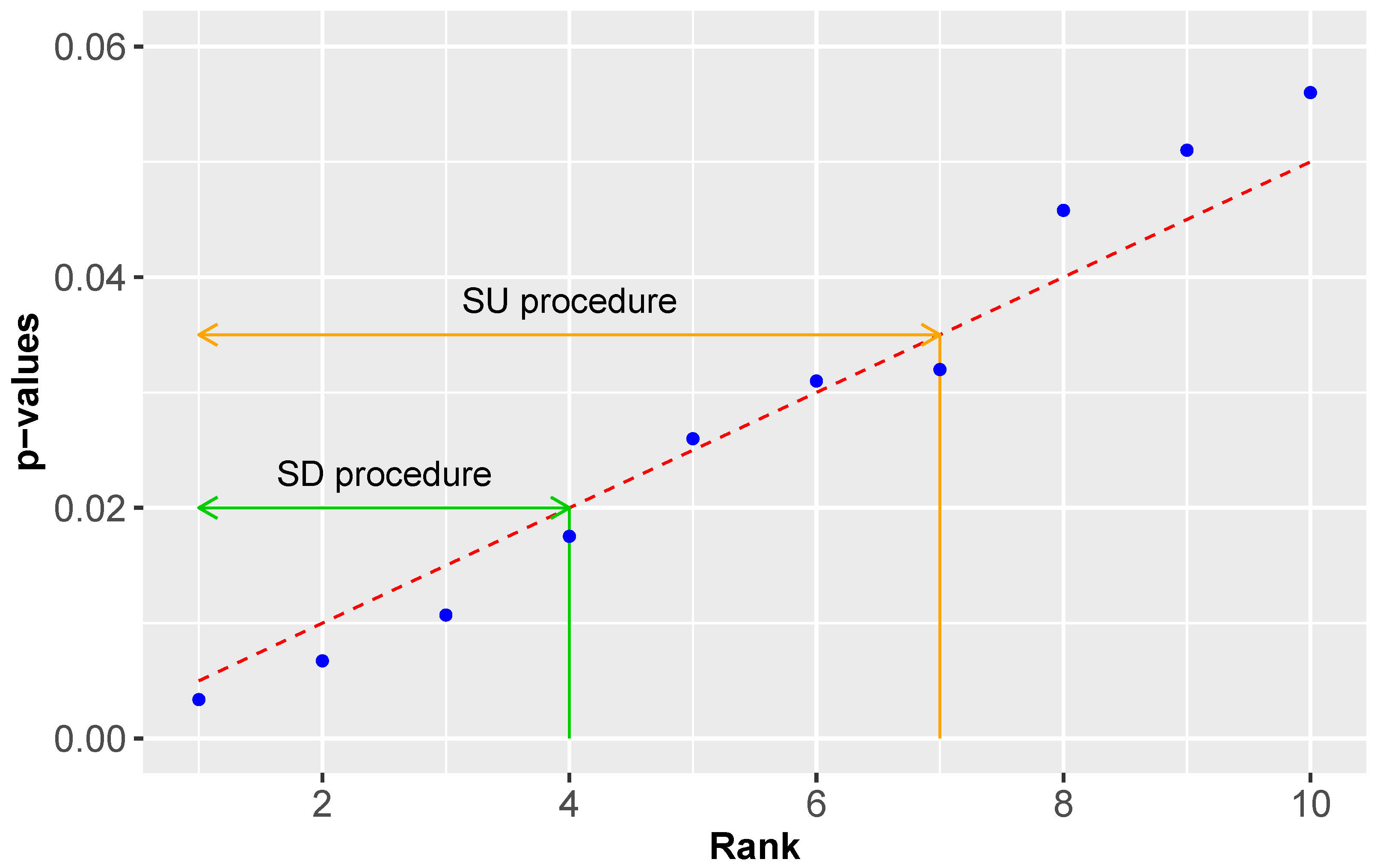
4.1. Single-Step vs. Stepwise Approaches

Overall, there are three different types of MTPs commonly distinguished by the way they conceptually compare p-values with critical values [55].

• Single-step (SS) procedure
• Step-up (SU) procedure
• Step-down (SD) procedure

The SU and SD procedures are commonly referred to as stepwise procedures.

Assuming we have ordered p-values as given by Equation (2) then the procedures are defined as follows.

Definition 3. Single-step (SS) procedure:

A SS procedure tests the condition

$$\begin{array}{c}\hfill p_{(i)}\le c_i\end{array}$$

(27)

and rejects the null hypothesis i if this condition holds.

For a SS procedure there is no order needed in which the conditions are tested. Hence, previous decisions are not taken into consideration. Furthermore, usually, the critical values $c_i$ are constant for all tests, i.e., $c_i=c$ for all i.

Definition 4. Step-up (SU) procedure:

Conceptually, a SU procedure starts from the least significant p-value, $p_{(m)}$, and goes toward the most significant p-value, $p_{(1)}$, by testing successively if the condition

$$\begin{array}{c}\hfill p_{(i)}\le c_i\end{array}$$

(28)

holds. For the first index $i^{*}$ for which this condition holds the procedure stops and rejects all null hypothesis j with $j\le i^{*}$, i.e., reject the null hypotheses

$$\begin{array}{c}\hfill H_{(1)},H_{(1)},\dots ,H_{(i^{*})}.\end{array}$$

(29)

If such an index does not exist do not reject any null hypothesis.

Formally, a SU procedure identifies the index

$$\begin{array}{c}\hfill i^{*}=max\left\{i\in \{1,\dots ,m\}|p_{(i)}\le c_i\right\}\end{array}$$

(30)

for the critical values $c_i$. Usually, the $c_i$s are not constant but change with index i.

Definition 5. Step-down (SD) procedure:

Conceptually, a SU procedure starts from the most significant p-value, $p_{(1)}$, and goes toward the least significant p-value, $p_{(m)}$, by testing successively if the condition

$$\begin{array}{c}\hfill p_{(i)}\le c_i\end{array}$$

(31)

holds. For the first index $i^{*}+1$ for which this conditiondoes not holdthe procedure stops. Then it rejects all null hypothesis j with $j\le i^{*}$, i.e., reject the null hypotheses

$$\begin{array}{c}\hfill H_{(1)},H_{(1)},\dots ,H_{(i^{*})}.\end{array}$$

(32)

If such an index does not exist do not reject any null hypothesis.

Formally, a SD procedure identifies the index

$$\begin{array}{c}\hfill i^{*}=max\left\{i\in \{1,\dots ,m\}|p_{(j)}\le c_j,\mathrm{for}\mathrm{all}j\in \{1,\cdots ,i\}\right\}\end{array}$$

(33)

for the critical values $c_i$.

Regarding the meaning of both procedures, we want to make two remarks. First, we would like to remark that the direction, either ‘up’ or ‘down’, is meant with respect to the significance of p-values. That means a SU procedure steps toward more significant p-values (hence it steps up) whereas a SD procedure steps toward less significant p-values (hence it steps down).

Second, the crucial difference between a SU procedure and a SD procedure is that a SD procedure is more strict requiring all p-values below $i^{*}$ to be significant as well whereas a SU procedure does not require this.

In Figure 2 we visualize the working mechanism of a SD and a SU procedure. The dashed red line corresponds to the critical values $c_i$ and the blue points to rank ordered p-values. Whenever a p-value is below the dashed red line its corresponding null hypothesis is rejected, otherwise accepted. The green range indicates p-values identified with a SD procedure whereas the orange range indicates p-values identified with a SU procedure. As one can see, a SU procedure is less conservative than a SD procedure because it does not have the monotonicity requirement.

4.2. Adaptive vs. Non-Adaptive Approaches

Another way to categorize MTPs is if they estimate the number of null hypotheses $m_0$ from the data or not. The former type of procedures is called adaptive procedures (AD) and the latter ones non-adaptive (NA) [56,57]. Specifically, adaptive MTP estimate the number of null hypotheses $m_0$ from a given data set and then use this estimate for a multiple test procedure. In contrast, NA MTP assume $m_0=m$.

4.3. Marginal vs. Joint Multiple Testing Procedures

A third way to categorize MTPs is if they are using marginal or joint distributions of the test statistics. Multivariate procedures are capable of taking into account the dependency structure in the data (among the test statistics) and, hence, such MTPs can be more powerful than marginal procedures because the latter just ignore this information. For instance, the dependency structure manifests as a correlation structure which can have a noticeable effect on the results.

Usually, procedures using joint distributions are based on resampling approaches, e.g., Bootstrapping or permutations [10,22]. Hence, they are nonparametric methods which require computational approaches.

5. Controlling the FWER

We start our presentation of MTPs with methods for controlling the FWER [58]. In the following, we will discuss procedures from Šidák, Bonferroni, Holm, Hochberg, Hommel, and Westfall-Young. This discussion emphasizes the working mechanisms behind the procedures. In Section 8 we present a summary of the underlying assumptions the procedures rely on.

5.1. Šidák Correction

The first MTP we discuss for controlling the FWER has been introduced by Šidák [21]. Let’s say we want to control the FWER at a level $\alpha$. If we reverse Equation (26) we obtain an adjusted significance level given by

$$\begin{array}{c}\hfill {\alpha }_S=1-{(1-\alpha )}^{1/m}.\end{array}$$

(34)

This equation allows calculation of the corresponding adjusted significance level ${\alpha }_S$ of the individual hypotheses for every FWER of $\alpha$ and every m (number of hypotheses). A null hypothesis $H_i$ is rejected if

$$\begin{array}{c}\hfill p_i\le {\alpha }_S\end{array}$$

(35)

holds. Hence, by using ${\alpha }_S(m)$ the FWER is controlled at level $\alpha$.

The procedure given by Equation (35) is called single-step Šidák correction. For completeness we also want to mention that there is a SD Šidák correction defined by

$$\begin{array}{c}\hfill p_i\le 1-{(1-\alpha )}^{1/m-i+1}.\end{array}$$

(36)

From Equations (34) and (35) we can derive adjusted p-values for the single-step Šidák correction which are given by

$$\begin{array}{c}\hfill p_i^{adj}=min\{1-{(1-p_i)}^m,1\}\end{array}$$

(37)

These adjusted p-values can alternatively be used to test for significance by comparing them with the original significance level, i.e.,

$$\begin{array}{c}\hfill p_i^{adj}\le \alpha .\end{array}$$

(38)

In Figure 3A, we show the adjusted significance level ${\alpha }_S$ of the individual hypotheses for a single-step Šidák correction in dependence on the number of hypotheses m for $\alpha =0.05$. As one can see, the adjusted significance level ${\alpha }_S$ becomes quickly more stringent for an increasing number of hypothesis tests m.

5.2. Bonferroni Correction

The Bonferroni correction controls the FWER under general dependence [17]. From a Taylor expansion of Equation (34) up to the linear term, we obtain the following approximation given by

$$\begin{array}{c}\hfill {\alpha }_B=\frac{\alpha }{m}.\end{array}$$

(39)

By using Boole’s inequality one can elegantly show that this controls the FWER [50].

Equation (39) is the adjusted Bonferroni significance level. We can use this adjusted significance level to test every p-value and reject the null hypothesis $H_i$ if

$$\begin{array}{c}\hfill p_i\le {\alpha }_B.\end{array}$$

(40)

From Equations (39) and (40) we can derive adjusted p-values which are given by

$$\begin{array}{c}\hfill p_i^{adj}=min\{m{p}_i,1\}.\end{array}$$

(41)

These adjusted p-values can alternatively be used to test for significance by comparing them with the original significance level, i.e.,

$$\begin{array}{c}\hfill p_i^{adj}\le \alpha .\end{array}$$

(42)

The result of this is shown in Figure 3. Specifically, the FWER in Equation (26) is shown for the corrected significance level ${\alpha }_B$ given by

$$\begin{array}{c}\hfill \mathrm{FWER}=1-{(1-{\alpha }_B)}^m.\end{array}$$

(43)

As one can see, the FWER is for all m controlled because it is always below $\alpha =0.05$. Here it is important to emphasize that the y-axis range is only from $0.048$ to $0.05$ to see the effect.

5.3. Holm Correction

A modified Bonferroni correction has been suggested by [23], called the Holm correction. In contrast to a Bonferroni correction, but also Sidak, it is a sequential procedure that tests ordered p-values. For this reason, it has also been also called ‘the sequentially rejective Bonferroni test’ [23].

Let us indicate by

$$\begin{array}{c}\hfill p_{(1)}\le p_{(2)}\cdots \le p_{(m)}\end{array}$$

(44)

the ordered sequence of p-values in increasing order. Then the Holm correction tests the following conditions in a SD manner:

$$\begin{array}{ccc}\hfill \mathrm{Step}1.:\mathrm{Reject} H_{(1)} \mathrm{if} p_{(1)}& \le & \frac{\alpha }{m}\hfill \end{array}$$

(45)

$$\begin{array}{ccc}\hfill \mathrm{Step}2.:\mathrm{Reject} H_{(2)} \mathrm{if} p_{(2)}& \le & \frac{\alpha }{m-1}\hfill \end{array}$$

(46)

$$\begin{array}{ccc}\hfill \mathrm{Step}3.:\mathrm{Reject} H_{(3)} \mathrm{if} p_{(3)}& \le & \frac{\alpha }{m-2}\hfill \\ & ⋮& \end{array}$$

(47)

$$\begin{array}{ccc}\hfill \mathrm{Step}m.:\mathrm{Reject} H_{(m)} \mathrm{if} p_{(m)}& \le & \frac{\alpha }{1}\hfill \end{array}$$

(48)

If at any step the $H_{(i)}$ is not rejected, the procedure stops and all other p-values, i.e., $p_{(i)},p_{(i+1)},\dots p_{(m)}$ are accepted. Compactly, the above testing criteria of the steps can be written as

$$\begin{array}{c}\hfill p_{(i)}\le \frac{\alpha }{m-i+1}\end{array}$$

(49)

for $i\in \{1,\dots ,m\}$. As one can see, the first step, i.e., $i=1$, is exactly a Bonferroni correction and each following step is in the same spirit but considering the changed number of remaining tests. The optimal cut-off index of this SD procedure can be identified by

$$\begin{array}{c}\hfill i^{*}=max\left\{i\in \{1,\dots ,m\}|p_{(j)}\le \frac{\alpha }{m-j+1},\mathrm{for} \mathrm{all} j\in \{1,\dots ,i\}\right\}.\end{array}$$

(50)

From this the adjusted p-values of a Holm correction can be derived [12] and are given by

$$\begin{array}{c}\hfill p_{(i)}^{adj}=\underset{j\le i}{max}\left\{\underset{k\in \{1,\dots ,j\}}{min}\left\{(m-k+1)p_{(k)},1\right\}\right\}.\end{array}$$

(51)

The nested character of this formulation comes from the strict requirement of a SD procedure that all p-values, $p_{(i)}$, need to be significant with $j\le i$ (see the j index in Equation (50)). An alternative, more explicit form to obtain the adjusted p-values is given by the following sequential formulation [59]:

$$\begin{array}{c}\hfill p_{(i)}^{adj}=\left\{\begin{array}{c}min\{m{p}_{(i)},1\}\mathrm{if}i=1\hfill \\ max\{p_{(i-1)}^{adj},(m-i+1)p_{(i)}\}\mathrm{if}i=\{2,\dots ,m\}\hfill \end{array}\right.\end{array}$$

(52)

A computational realization of a Holm correction is given by Algorithm 1.

Algorithm 1: SD Holm correction procedure.

Input: $p_{(1)}\le p_{(2)}\cdots \le p_{(m)}$  1 $k=0$  2 while $p_{(k+1)}\le \alpha /(m-k)$ do  3 $⎿$ $k=k+1$  4 Reject $H_{(1)},H_{(1)},\dots H_{(k)}$

Similar to a Bonferroni correction, also Holm does not require the independence of the test statistics and provides a strong control of the FWER. In general, this procedure is more powerful than a Bonferroni correction.

5.4. Hochberg Correction

Another MTC that is formally very similar to the Holm correction is the Hochberg correction [24], shown in Algorithm 2. The only difference is that it is a SU procedure.

Algorithm 2: SU Hochberg correction procedure

Input: $p_{(1)}\le p_{(2)}\cdots \le p_{(m)}$  1 $k=m$  2 while $p_{(k)}>\alpha /(m-k+1)$ do  3 $⎿$ $k=k-1$  4 Reject $H_{(1)},H_{(1)},\dots H_{(k)}$

The adjusted p-values of the Hochberg correction are given by [59]:

$$\begin{array}{c}\hfill p_{(i)}^{adj}=\left\{\begin{array}{c}{p}_{(i)}\mathrm{if}i=m\hfill \\ min\{p_{(i+1)}^{adj},(m-i+1)p_{(i+1)}\}\mathrm{if}i=\{m-1,\dots ,2\}\hfill \end{array}\right.\end{array}$$

(53)

The Hochberg correction is an optimistic approach because it tests backwards, and it stops as soon as a p-value is significant at level $\alpha /(m-k+1)$. The SU character makes it more powerful and, hence, the SU Hochberg procedure is more powerful than the SD Holm procedure.

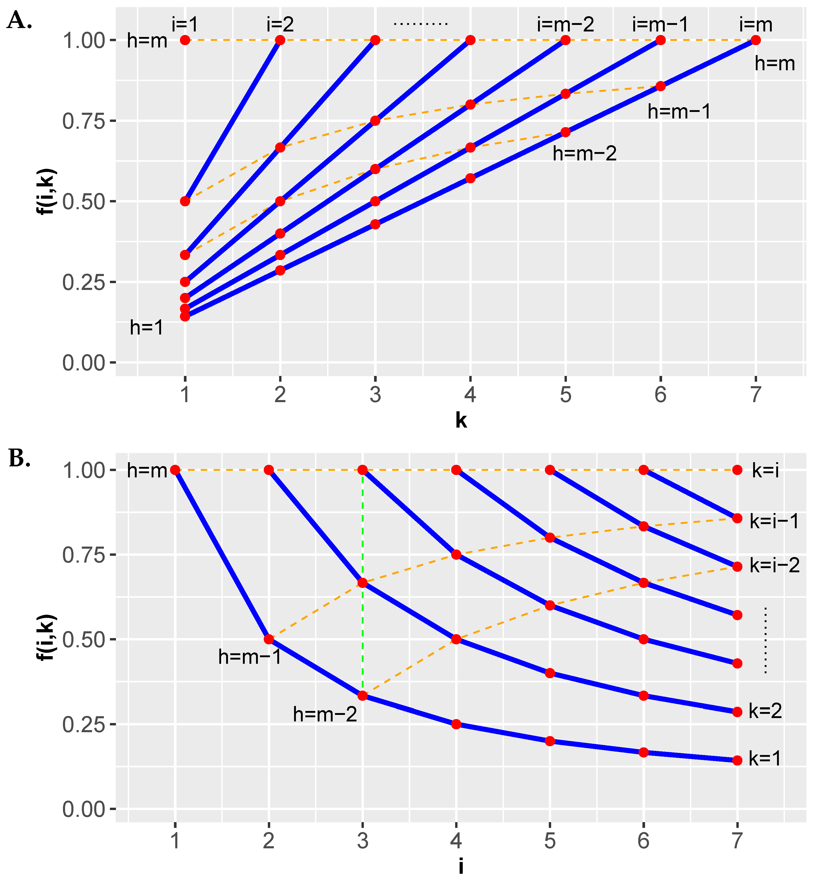
5.5. Hommel Correction

The next MTP we discuss, the Hommel correction [60], is far more complex than the previous procedures. The method evaluates the set

$$\begin{array}{c}\hfill i^{*}=max\left\{i\in \{1,\dots ,m\}|p_{(m-i+k)}>\frac{k}{i}\alpha , \mathrm{for} \mathrm{all} k\in \{1,\dots ,i\}\right\}\end{array}$$

(54)

and determines the maximum index for which this condition holds [28]. If such an index does not exist, then we reject $H_{(1)},H_{(1)},\dots H_{(m)}$ otherwise we reject only the p-values for which holds

$$\begin{array}{c}\hfill p<\frac{\alpha }{i^{*}}.\end{array}$$

(55)

In Figure 4 we visualize the testing condition for $m=7$. In this figure the scaling factor $f(i,k)=k/i$ is shown in dependence on the index i and k. Each red point corresponds to an index pair $(i,k)$. Figure 4A shows $f(i,k)$ for fixed i values and Figure 4B shows $f(i,k)$ for fixed k values. This leads to k respectively i dependent curves shown in blue, i.e., $f(i \mathrm{fixed}, k)$ and $f(i,k \mathrm{fixed})$. In both figures, the isolines shown as orange dashed lines, connect points with a constant index $h=m-i+k$. For each blue line (in both figures) the points on these lines have indices $h=m$, $h=m-1$ etc. going from high to low values of $f(i,k)$. These indices are used for the rank ordered p-values, i.e.,

$$\begin{array}{c}\hfill p_{(h)}=p_{(m-i+k)}.\end{array}$$

(56)

According to Equation (54), for each index i there are i different values of k. In Figure 4A these correspond to the points on the blue lines and in Figure 4B these correspond to the points in vertical columns. In Figure 4B we highlight just one of these as a green dashed line.

The following array in Equation (57) shows for each step of the procedure the corresponding conditions that need to be tested. At Step 1, the index $i=m$. For reasons of simplicity we use the notation $F(i,k)=f(i,k)\alpha =k\alpha /i$. Only if all conditions for a step (for a column) are true, the procedure stops and $i^{*}$ corresponds to the i value of this step. Otherwise the procedure continues to the next step.

$$\begin{array}{c}\hfill \begin{array}{cccccc}Step:& 1& 2& \dots & m-1& m\\ i:& m& m-1& \dots & 2& 1\\ & p_{(m)}>F(m,m)& p_{(m)}>F(m-1,m-1)& \dots & p_{(m)}>F(2,2)& p_{(m)}>F(1,1)\\ & p_{(m-1)}>F(m,m-1)& p_{(m-1)}>F(m-1,m-2)& \dots & p_{(m-1)}>F(2,1)& \\ & ⋮& ⋮& & & \\ & p_{(3)}>F(m,3)& p_{(3)}>F(m-1,2)& & & \\ & p_{(2)}>F(m,2)& p_{(2)}>F(m-1,1)& & & \\ & p_{(1)}>F(m,1)& & & & & \end{array}\end{array}$$

(57)

As one can see from the triangular shaped array, the number of conditions per step decreases by one. Specifically, always the smallest p-value from the previous step is dropped. This increased the probability for all conditions to hold from step to step because also the corresponding values of $F(i,k)$ increase. Specifically, $F(c,d)<F(c-1,d)$ hold for all c because

$$\begin{array}{c}\hfill \frac{d\alpha }{c}<\frac{d\alpha }{c-1}\end{array}$$

(58)

holds for all c. Hence, the smallest p-values tested per step are compared to decreasingly stringent conditions.

In algorithmic form, one can write the Hommel correction as shown in Algorithm 3. In this form the Hommel correction is less compact but easier to understand. It has been found that the Hommel procedure is more powerful than Bonferroni, Holm and Hochberg [28]. Finally, we want to mention that very recently a much faster computational realization has been found [44]. This algorithm has a linear time complexity and leads to an astonishing improvement allowing the application to millions of tests.

Algorithm 3: Hommel correction procedure

Input: $p_{(1)}\le p_{(2)}\cdots \le p_{(m)}$  1 $i=m$  2 while $p_{(m-i+k)}\le \frac{k}{i}\alpha$ for at least one $k\in \{1,\cdots ,i\}$ do  3 $⎿$ $i=i-1$  4 $i^{*}=i$  5 if $i^{*}=0$ then  6 $⎿$ Reject $H_{(1)},H_{(1)},\dots H_{(m)}$  7 else  8 $⎿$ Reject $H_{(l)}$ with $p_l<\frac{\alpha }{i^{*}}$

5.5.1. Examples

Let us consider some numerical examples for $m=5$. In this case, the general array in Equation (57) assumes the following numerical values.

$$\begin{array}{c}\begin{array}{cccccc}Step:& 1& 2& 3& 4& 5\\ i:& 5& 4& 3& 2& 1\\ & p_{(5)}>0.05& p_{(5)}>0.05& p_{(5)}>0.05& p_{(5)}>0.05& p_{(5)}>0.05\\ & p_{(4)}>0.04& p_{(4)}>0.037& p_{(4)}>0.033& p_{(4)}>0.025& \\ & p_{(3)}>0.03& p_{(3)}>0.025& p_{(3)}>0.016& & \\ & p_{(2)}>0.02& p_{(2)}>0.012& & & \\ & p_{(1)}>0.01& & & & \end{array}\end{array}$$

(59)

• Example 1: $p_{(1)}=0.011,p_{(2)}=0.021,p_{(3)}=0.031,p_{(4)}=0.41,p_{(5)}=0.051$. In this case, $i^{*}=5$ and $\alpha /i^{*}=0.01$. From this follows that no hypothesis can be rejected.
• Example 2: $p_{(1)}=0.009,p_{(2)}=0.021,p_{(3)}=0.031,p_{(4)}=0.41,p_{(5)}=0.051$. In this case, $i^{*}=4$ and $\alpha /i^{*}=0.0125$. From this it follows that $H_{(1)}$ can be rejected.
• Example 3: $p_{(1)}=0.009,p_{(2)}=0.021,p_{(3)}=0.024,p_{(4)}=0.41,p_{(5)}=0.051$. In this case, $i^{*}=3$ and $\alpha /i^{*}=0.016$. From this it follows that $H_{(1)}$ can be rejected.

These examples should demonstrate that the application and outcome of a Hommel correction is non-trivial.

5.6. Westfall-Young Procedure

For most real-world situations, the joint distribution of the test statistics is unknown. Westfall and Young made seminal contributions by showing that in this case resampling-based methods can be used, under certain conditions, to estimate p-values without the need for making many theoretical assumptions [22]. However, in order to do this one needs (1) access to the data and (2) be able to resample the data in such a way that the resulting permutations allow estimation of the null hypotheses of the test statistics. The latter is usually possible for two-sample tests but may be more involved for other types of tests.

In particular, four such permutation-based methods have been introduced by Westfall and Young [22]. Two of these are single-step procedures and two are SD procedures. The single-step procedures are called single-step minP

$$\begin{array}{c}\hfill {\tilde{p}}_j=Pr\left(\underset{l\in \{1,\dots ,m\}}{min}{P}_l\le p_j|H_0^C\right)\end{array}$$

(60)

and single-step maxT

$$\begin{array}{c}\hfill {\tilde{p}}_j=Pr\left(\underset{l\in \{1,\dots ,m\}}{max}|T_l|\ge t_j|H_0^C\right)\end{array}$$

(61)

and their adjusted p-values are given by the above Equations (60) and (61). Here $H_0^C$ is an intersection of all true null hypotheses, $P_l$ denotes unadjusted p-values from permutations and $T_l$ denotes test statistics from permutations. The $p_j$ and $t_j$ are the p-values and test statistics from the un-permuted data.

Without additional assumptions, single-step maxT and single-step minP provide a weak control of the FWER. However, for subset pivotality both procedures control the FWER strongly [22]. Here subset pivotality is a property of the distribution of raw p-values and holds if all subsets of p-values have the identical joint distribution under the complete null distribution [10,22,61] (for a discussion of an alternative an practically simpler sufficient condition see [62]). Furthermore, the results from single-step maxT and single-step minP give the same results when the test statistics are identically distributed [49].

From a computational perspective, the single-step minP is computationally more demanding than the single-step maxT because it is based on p-values and not on test statistics. The difference is that one can get a resampled value of a test statistic from one resampled data set whereas for a p-value one needs a distribution of resampled test statistics which can only be obtained from many resampled data sets. This has been termed double permutation [63].

The SD procedures are called SD minP

$$\begin{array}{c}\hfill {\tilde{p}}_{r_j}=\underset{k\in 1,\dots ,j\}}{max}\left\{Pr\left(\underset{l\in \{k,\dots ,m\}}{min}{P}_{r_l}\le p_{r_k}|H_0^C\right)\right\}\end{array}$$

(62)

and SD maxT

$$\begin{array}{c}\hfill {\tilde{p}}_{s_j}=\underset{k\in 1,\dots ,j\}}{max}\left\{Pr\left(\underset{l\in \{k,\dots ,m\}}{max}|T_{s_l}|\ge t_{s_k}|H_0^C\right)\right\}\end{array}$$

(63)

and their adjusted p-values are given by the above Equations (62) and (63). The indices $r_k$ and $s_k$ are the ordered indices, i.e., $|t_{s_1}|\ge |t_{s_2}|\ge \cdots \ge |t_{s_m}|$ and $p_{r_1}\le p_{r_2}\le \cdots \le p_{r_m}$.

Interestingly, it can be shown that assuming the $P_l$ are uniformly distributed in $[0,1]$ the p-values in Equation (62) correspond with the ones obtained from the Holm procedure [63]. That means in general the SD minP procedure is less conservative than Holm’s procedure. Again, the SD minP is computationally more demanding than the SD maxT because of the required double permutations. Also, assuming subset pivotality both procedures have a strong control of the FWER [64].

The general advantage of using maxT and minP procedures over all other procedures discussed in our paper is that these use potentially the dependency structure among the test statistics. That means when such a dependency (correlation) is absent there is no apparent need for using these procedures. However, most data sets have some kind of dependency since the associated covariates are usually connected with each other. In such situations, the maxT and minP procedures can lead to an improved power.

In algorithmic form, the SD maxT and SD minP procedure can be formulated as shown in Algorithms 4 and 5. For Step 2 in Algorithm 5, it is important to point out that the estimates of the raw p-value $p_{i,b}$ are obtained for the same permutations obtained in Step 1.

Algorithm 4: Westfall-Young step-down maxT procedure.

Algorithm 5: Westfall-Young step-down minP procedure.

6. Controlling the FDR

Now we come to a second type of correction methods. In contrast to the methods discussed so far controlling the FWER, the methods we are discussing in the next sections are controlling the FDR. That means these methods have a different optimization goal. In Section 8 we present a summary of the underlying assumptions the procedures rely on.

6.1. Benjamini-Hochberg Procedure

The first method from this category we discuss controlling the FDR is called the Benjamini-Hochberg (BH) procedure [19]. The BH procedure can be considered a breakthrough method because it introduced a novel way of thinking to the community. The procedure assumes ordered p-values as in Equation (44). Then it identifies by a SU procedure the largest index k for which

$$\begin{array}{c}\hfill p_{(i)}\le i\frac{\alpha }{m}\end{array}$$

(66)

holds and rejects the null hypotheses $H_{(1)},H_{(2)},\dots ,H_{(k)}$. Compactly, this can be formulated by

$$\begin{array}{c}\hfill k=max\left\{i\in \{1,\dots ,m\}|p_{(i)}\le i\frac{\alpha }{m}\right\}.\end{array}$$

(67)

If no such index exists then no hypothesis is rejected.

Conceptually, the BH procedure uses Simes inequality [37], see Section 2.1. In algorithmic form, the BH procedure can be formulated as shown in Algorithm 6.

Algorithm 6: SU Benjamini-Hochberg procedure

Input: $p_{(1)}\le p_{(2)}\cdots \le p_{(m)}$  1 $k=0$  2 while $p_{(k+1)}\le ((k+1)\alpha )/m$ do  3 $⎿$ $k=k+1$  4 Reject $H_{(1)},H_{(1)},\dots H_{(k)}$

The adjusted p-values of the BH procedure are given by [49]

$$\begin{array}{c}\hfill p_{(i)}^{adj}=\underset{j\in \{1,\dots ,m\}}{min}\left\{\frac{m{p}_{(j)}}{j},1\right\}.\end{array}$$

(68)

In general, the BH procedure makes a good trade-off between false positives and false negatives and works well for independent test statistics or positive regression dependencies (denoted by PRDS) which is a weaker assumption than independence [25,57,65]. Generally, it is also more powerful than procedures controlling the FWER. The correlation assumptions imply that in the presence of negative correlations the control of the FDR is not always achieved. Also, the BH procedure can suffer from a weak power, especially when testing a relatively small number of hypotheses because in such a situation it is similar to a Bonferroni correction, see Figure 5B.

6.1.1. Example

In Figure 5 we show a numerical example for the BH procedure. In Figure 5A we show $m=100$ rank ordered p-values. The dashed red line corresponds to a significance level of $\alpha =0.05$ and the dashed green line corresponds to the testing condition in Equation (66).

In Figure 5B we zoom into the first 30 p-values. Here we also added a Bonferroni correction as dashed orange line at a value of $\alpha /m=5e-04$. One can see that the BH correction corresponds to a straight line that is always above the Bonferroni correction. Hence, a BH is always less conservative than a Bonferroni correction. As a result, for the shown p-values we obtain 18 significant values for the BH correction but only 3 significant values for the Bonferroni correction. One can also see that using the uncorrected p-values with $\alpha =0.05$ gives additional significant values in an uncontrolled manner beyond rank 18.

6.2. Adaptive Benjamini-Hochberg Procedure

In [56] a modified version of the BH procedure has been introduced which estimates the proportion of null hypothesis, ${\pi }_0$ from data whereas the proportion of true null hypotheses is given by ${\pi }_0=m_0/m$. For this reason, this procedure is called adaptive Benjamini-Hochberg procedure (adaptive BH).

The adaptive BH procedure modifies Equation (66) by substituting $\alpha$ with $\alpha /{\pi }_0$ which gives

$$\begin{array}{c}\hfill p_{(i)}\le =i\frac{\alpha }{{\pi }_{0}m}=i\frac{\alpha }{m_0}.\end{array}$$

(69)

The procedure itself searches in a SU manner the larges index k for which

$$\begin{array}{c}\hfill k=max\left\{i\in \{1,\dots ,m\}|p_{(i)}\le i\frac{\alpha }{{\pi }_{0}m}\right\}\end{array}$$

(70)

holds. If no such index exists then no hypothesis is rejected, otherwise reject the null hypotheses $H_{(1)},H_{(2)},\dots ,H_{(k)}$.

The estimator for ${\pi }_0$ is found as a result from an iterative search based on [66]

$$\begin{array}{c}\hfill {\widehat{\pi }}_0^{BH}(k)=\frac{m-k+1}{(1-p_{(k)})m}.\end{array}$$

(71)

Specifically, the optimal index k is found from

$$\begin{array}{c}\hfill k=min\left\{i\in \{2,\dots ,m\}|{\widehat{\pi }}_0^{BH}(i)>{\widehat{\pi }}_0^{BH}(i-1)\right\}.\end{array}$$

(72)

The importance of this study does not lie in its practical usage but in the inspiration it provided for many follow-up approaches that introduced new estimators for ${\pi }_0$. In this paper, we will provide some examples for this, e.g., when discussing the BR-2S procedure and in the summary Section 8.

6.3. Benjamini-Yekutieli Procedure

To improve the BH procedure that can deal with a dependency structure, in [25] a modification has been introduced, called the Benjamini-Yekutieli (BY) procedure. The BY procedure assumes also ordered p-values as in Equation (44) and then it identifies in a stepwise procedure the largest index k for which

$$\begin{array}{c}\hfill p_{(k)}\le k\frac{\alpha }{mf(m)}\end{array}$$

(73)

holds and rejects the null hypotheses $H_0^{(1)},H_0^{(2)},\dots ,H_0^{(k)}$. It is important to note that here the factor $f(m)={\sum }_{i=1}^{m}1/i$ is introduced which depends on the total number of hypotheses. Compactly, this can be formulated by

$$\begin{array}{c}\hfill k=max\left\{i\in \{1,\dots ,m\}|p_{(i)}\le i\frac{\alpha }{mf(m)}\right\}.\end{array}$$

(74)

If no such index exists then no hypothesis is rejected.

Since $f(m)>1$ for all m, the product $mf(m)$ can be seen as an effective increase in the number of hypotheses to $m^{\prime }$ with $m^{\prime }=mf(m)$. Hence, the BY procedure is very conservative and it can be even more conservative than a Bonferroni correction. For instance, for $m\in \{100,1000,\mathrm{10,000},\mathrm{100,000}\}$ we obtain $f(m)=\{5.8,7.5,9.8,12.1\}$. The adjusted p-values of the BY procedure are given by [49]

$$\begin{array}{c}\hfill p_{(i)}^{adj}=\underset{k\in \{i,\dots ,m\}}{min}\left\{\frac{mf(m)p_{(k)}}{k},1\right\}.\end{array}$$

(75)

It has been proven that the BY procedure controls the FDR in the strong sense by

$$\begin{array}{c}\hfill FDR\le \frac{m_0}{m}\alpha ={\pi }_0\alpha \end{array}$$

(76)

for any type of dependent data [25]. Since it is always $m_0\le m$, the FDR is either controlled at level $\alpha$ (for $m_0=m$) or even below that level. A disadvantage of the BY procedure is that it is less powerful than BH.

6.3.1. Example

In Figure 6 we show a numerical example for the BY procedure. Here the BY correction corresponds to the dashed red line which is always below the BH correction (dashed green line) indicating that it is more conservative.

Interestingly, the line for the BY correction intersects with the Bonferroni correction (dashed orange line) at rank 5 (see inlay). That means below this value the BY correction is more conservative and after the intersection less conservative. For the p-values in this example, the BY gives no significant results. This indicates the potential problem with the BY procedure in practice because its conservativeness can lead to no significant results at all.

6.4. Benjamini-Krieger-Yekutieli Procedure

Yet another modification of the BH procedure has been introduced in [26]. This MTP is an adaptive two-stage linear SU method, called BKY (Benjamini-Krieger-Yekutieli). Here ‘adaptive’ means that the procedure estimates the number of null hypothesis from the data and uses this information to improve the power. This approach is motivated by Equation (76) and the dependency of the control on $m_0$.

Step 1:

Use a BH procedure with ${\alpha }^{\prime }=\alpha /(1-\alpha )$. Let r be the number of hypotheses rejected. If $r=0$, no hypothesis is rejected. If $r=m$ reject all m hypotheses. In both cases, the procedure stops. Otherwise proceed.

Step 2:

Estimate the number of null hypotheses by $\widehat{m_0}=m-r$.

Step 3:

Use a BH procedure with ${\alpha }^{″}=m{\alpha }^{\prime }/(\widehat{m_0})={\alpha }^{\prime }/{\widehat{\pi }}_0$.

The BKY procedure uses the BH procedure twice. In the first stage to estimate the number of null hypotheses $\widehat{m_0}$ and in the second to declare significance.

The BKY procedure controls the FDR exactly at level $\alpha$ when tests are independent. In [26] it has been shown that this procedure has higher power than BH.

6.5. Blanchard-Roquain Procedure

A generalization of the BY procedure has been introduced by Blanchard & Roquain [67].

6.5.1. BR-1S Procedure

The first procedure introduced in [67] is a one-state adaptive SU procedure, called BR-1S, independently proposed in [57]. Formally, the BR-1S procedure [67], first, defines an adaptive threshold by

$$\begin{array}{c}\hfill t_{(i)}=min\left\{\lambda ,\frac{i\alpha (1-\lambda )}{m-i+1}\right\}\end{array}$$

(77)

for $\lambda \in (0,1)$ and for all $i\in \{1,\dots ,m\}$. Then the largest index k is determined for which holds

$$\begin{array}{c}\hfill k=max\left\{i\in \{1,\dots ,m\}|p_{(i)}\le t_{(i)}\right\}.\end{array}$$

(78)

If no such index exists then no hypothesis is rejected otherwise all null hypotheses with p-values with $p_{(i)}\le t_{(k)}$ are rejected.

For the BR-1S procedure it has been proven that the FDR is controlled by

$$\begin{array}{c}\hfill \mathrm{FDR}\le min\left\{\lambda ,\alpha (1-\lambda )m\right\}.\end{array}$$

(79)

A brief calculation shows that both arguments of the above Equation are equal for

$$\begin{array}{c}\hfill \lambda (m)=\frac{\alpha m}{1+\alpha m}.\end{array}$$

(80)

A further calculation shows that Equation (80) is monotonously increasing for increasing values of m and for $m\ge 2$ we find $\lambda (m)>\alpha$. That means one needs to choose $\lambda$ values smaller than the value on the right-hand side in Equation (80) to be able to control the FDR [67]. Hence, a common choice for $\lambda$ in Equation (79) is $\lambda =\alpha$ because this controls the FDR on the $\alpha$ level, i.e., $FDR\le \alpha$.

For $\lambda =\alpha$ the adaptive threshold simplifies and becomes

$$\begin{array}{c}\hfill t_{(i)}=\alpha min\left\{1,\frac{i(1-\alpha )}{m-i+1}\right\}.\end{array}$$

(81)

Furthermore, for $i\le (m+1)/2$ the adaptive threshold simplifies even further to

$$\begin{array}{c}\hfill t_{(i)}=\alpha \frac{i(1-\alpha )}{m-i+1}.\end{array}$$

(82)

6.5.2. BR-2S Procedure

The second procedure introduced in [67] is a two-state adaptive plug-in procedure, called BR-2S, given by:

Stage 1:

Estimate $R({\lambda }_1)=m_0$ by BR-1S$({\lambda }_1)$.

Stage 2:

Use ${\alpha }^{\prime }=\alpha /{\widehat{\pi }}_0$ with

$$\begin{array}{c}\hfill {\widehat{\pi }}_0^{BR}=\frac{m-R({\lambda }_1)+1}{(1-{\lambda }_2)m}\mathrm{for}{\lambda }_2\in (0,1)\end{array}$$

(83)

in the SU procedure given by Equation (70). That means the estimate for the proportion of null hypotheses is used to find the larges index k for which

$$\begin{array}{c}k=max\{i\in \{1,\dots ,m\}|p_{(i)}\le i\frac{\alpha }{{\widehat{\pi }}_0^{BR}m}\}\end{array}$$

(84)

holds. If no such index exists then no hypothesis is rejected, otherwise reject the null hypotheses $H_{(1)},H_{(2)},\dots ,H_{(k)}$.

The BR-2S procedure depends on two parameters denoted by ${\lambda }_1$ and ${\lambda }_2$. The first parameter is for BR-1S in stage one, whereas the second enters the estimate of the proportion of null hypotheses in stage two. It has been proven [67] that for setting ${\lambda }_1=\alpha /(1+\alpha +1/m)$ in Step 1 of the BR-2S procedure one obtains FDR $=\lambda$. This suggests setting $\lambda =\alpha$ in Step 2. The BR-1S and BR-2S procedure are proven to control the FDR for arbitrary dependence.

7. Computational Complexity

When performing MTCs for high-dimensional data the computation time required by a procedure can have an influence on its selection. For this reason, we present in this section a comparison of the computation time for different methods in dependence on the dimensionality of the data.

In the following, we apply the eight MTPs of Bonferroni, Holm, Hochberg, Hommel, BH, BY, Benjamini-Krieger-Yekutieli and Blanchard-Roquain to p-values of varying size $m\in$ {100, 1000, 10,000, 100,000}. In

Table 2. Average computation times for eight MTPs. The time unit is either seconds (s) or minutes (min). The Hommel algorithm indicated by * is a fast algorithm by [44].

Method	Error Control	$\mathit{m}=1000$	$\mathit{m}=\mathrm{10,000}$	$\mathit{m}=\mathrm{20,000}$	$\mathit{m}=\mathrm{50,000}$
Bonferroni	FWER	$9.360\times {10}^{-5}$ s	0.000389 s	0.001163 s	0.002932 s
Holm	FWER	$1.801\times {10}^{-4}$ s	0.001569 s	0.002897 s	0.012100 s
Hochberg	FWER	$1.716\times {10}^{-4}$ s	0.001430 s	0.003673 s	0.010471 s
Hommel	FWER	$5.394\times {10}^{-2}$ s	4.556661 s	23.389805 s	2.6053 min
Hommel *	FWER	$7.607\times {10}^{-4}$ s	0.001618 s	0.003035 s	0.008737 s
Benjamini-Hochberg	FDR	$2.955\times {10}^{-4}$ s	0.001260 s	0.003132 s	0.011276 s
Benjamini-Yekutieli	FDR	$2.264\times {10}^{-4}$ s	0.001168 s	0.004412 s	0.014482 s
Benjamini-Krieger-Yekutieli	FDR	$3.023\times {10}^{-3}$ s	0.025884 s	0.057175 s	0.147631 s
Blanchard-Roquain	FDR	$1.885\times {10}^{-3}$ s	0.024531 s	0.048221 s	0.126420 s

we show the mean computation times averaged over 10 independent runs.

One can see that there are large differences in the computation times. By far the slowest method is Hommel. For instance, correcting $m$ = 20,000 p-values takes over 20,000 times longer than for a Bonferroni correction. This method has also the worst scaling which means practical applications need to take this into consideration. This computational complexity could already be anticipated from our discussion in Section 5.5 because the Hommel correction is much more involved than all other procedures. However, the new algorithm by [44] (indicated by *) leads to an astonishing improvement in the computational complexity for this method.

Furthermore, from Table 2 one can see that we find essentially three groups of computational times. In the group of the fastest methods are Bonferroni, Holm, Hochberg, BH, and BY. In the medium fast group are Benjamini-Krieger-Yekutieli and Blanchard-Roquain and in the group of the slowest methods is only Hommel. Overall, the computation times of all methods in group one and two are very fast although the procedures by Benjamini-Krieger-Yekutieli and Blanchard-Roquain are ten times slower than the ones in group one.

8. Summary

In this paper, we reviewed MTPs for controlling either the FWER or the FDR. We emphasized their principal approach allowing categorization of them as (1) single-step vs. stepwise approaches, (2) adaptive vs. NA approaches, and (3) marginal vs. joint MTPs.

When it comes to the practical application of an MTP one needs to realize that to select a method there is more than the control of an error measure. Specifically, while a given MTP may guarantee the control of an error measure, e.g., the FWER or the FDR, this does not inform us about the Type 2 error/power of the procedure. In particular, the latter is for practical applications important because if one cannot reject any null hypothesis there is usually nothing to report or explore.

To find the optimal procedure for a given problem, the best approach is to conduct simulation studies comparing different MTPs. Specifically, for a given data set, one can diagnose its characteristics, e.g., by estimating the presence and the structure of correlations, and then simulate data following these characteristics. This ensure the simulations are problem-specific and adapt as close as possible to the characteristics of the data.

The advantage of this approach is that the selection of an MTP is not based on generic results from the literature but tailored to your problem. The disadvantage is the effort it takes to estimate, simulate, and compare the different procedures with each other.

If such a simulation approach is not feasible one needs to revert to results from the literature. In

Table 3. Summary of MTC procedures. PRDS denotes positive regression dependencies.

Method	Error Control	Procedure Type	Error Control Type	Correlation Assumed
Šidák	FWER	single-step	strong	non-negative
Šidák	FWER	step-down	strong	non-negative
Bonferroni	FWER	single-step	strong	any
Holm	FWER	step-down	strong	any
Hochberg	FWER	step-up	strong	PRDS
Hommel	FWER	step-down	strong	PRDS
maxT	FWER	single-step	strong	subset pivotality
minP	FWER	single-step	strong	subset pivotality
maxT	FWER	step-down	strong	subset pivotality
minP	FWER	step-down	strong	subset pivotality
Benjamini-Hochberg	FDR	step-up	strong	PRDS
Benjamini-Yekutieli	FDR	step-up	strong	any
Benjamini-Krieger-Yekutieli	FDR	step-up	strong	independence
BR-1S	FDR	step-up	strong	any
BR-2S	FDR	two-stage	strong	any

(and Figure 7 discussed below) we show a summary of MTPs and some important characteristics. Furthermore, from a multitude of simulation studies the following results have been found independently:

• Positive correlations (simulated data): BR is more powerful than BKY [67].
• General correlations (real data): BY has a higher PPV than BH [68].
• Positive correlations (simulated data): BKY is more powerful than BH [26].
• Positive correlations (simulated data): Hochberg, Holm and Hommel do not control the PFER for high correlations [69].
• General correlations (real data): SS MaxT has higher power than SS minP [49,70,71].
• General correlations (real data): SS MaxT and SD MaxT can be more powerful than Bonferroni, Holm and Hochberg [49].
• Random correlations (simulated data): SD minP is more powerful than SD maxT [71].

The above-mentioned simulation studies considered all the correlation structure in the data because this is of practical relevance. Since there is not just one type of a correlation structure that one needs to consider, the possible number of different studies is huge exploring all these different structures. Specifically, one can assume homogenous or heterogeneous correlations. The former assumes that pairwise correlations are equal throughout the different pairs whereas the latter assumes inequality. For heterogeneous correlation structures one can further assume a random structure or a particular structure. For instance, a particular structure can be imposed from an underlying network, e.g., a regulatory network among genes [72]. Hence, for the simulation of such data the covariance structure needs to be consistent with a structure of the underlying network [40].

Given all this information, how should one choose an MTP? In general, it is not necessarily suggested to select the MTP with the highest power. The reason follows from the evaluation of false positives (Type 1 errors) for a given situation. Whereas procedures controlling the FDR have in general a higher power than procedures controlling the FWER the latter can nevertheless be preferred when we need to be conservative in incurring false positives. For instance, in a clinical context such a false positive could correspond to a lethal outcome for the patient. In such a situation, an MTP with a smaller power but also a smaller Type 1 error is certainly preferred.

In this context, the study conducted by [69] is of interest because the authors compared MTPs controlling the FWER with further error measures (including the PFER). Their study underlines the need to consult always more than one error measure to judge the outcome; see also [73] for a general discussion of this problem.

In Figure 7 we show summarizing guidelines how to select an MTP. In the pre-selection steps (1–3) the number of available MTPs should be reduced by domain-specific knowledge. These steps include (1) the selection of an error measure, (2) the evaluation of the correlation structure of the data and (3) deciding if a marginal or joint multiple testing procedure is desired. This will lead to a reduced set of MTPs forming potential candidates. The MTPs within this reduced set are then thoroughly assessed either (4.A) by a simulation study or (4.B) by using information from the literature. Importantly, Step (4.A) requires the generation of simulated data with a similar correlation structure as the data to be analyzed. In addition, these simulated data should consider all relevant properties of the data to be analyzed. From Step (4.A) follows important information, e.g., about the power of an MTP that needs to be assessed in a domain-specific manner considering, e.g., the costs of Type 1 and Type 2 errors. Here the costs do not necessarily refer to financial burdens but and kind of negativity associated with these errors. This will allow a relevant assessment of the MTPs providing the most detailed information. If Step (4.A) cannot be carried out, Step (4.B) is applied. However, this step is only an approximative assessment compared to Step (4.A) because it relies on the availability of literature studies using data with properties close to the data to be analyzed. Based on this the most appropriate MTP is selected considering theoretical and domain-specific criteria.

One may wonder why it is necessary to conduct simulation studies for assessing the dependency of an MTP on the correlation structure in the data when, e.g., from Table 3 the assumed correlation is available. There are two reasons for this. First, the assumed correlation mentioned in Table 3, e.g., PRDS, relates to the correlation among p-values (or test statistics). Such a correlation could only be estimated from an ensemble of data sets, each independently identically generated. Hence, this is a theoretical property required for the mathematical proof of the control of an MTP that cannot be estimated from one data set alone. Second, even if one could estimate this one would not know what power an MTP achieves for a given data set. That means despite having a proven control of an MTP there is no information about its power in dependence on the correlation structure of a data set. Hence, this information needs to be obtained from simulation studies.

Overall, Figure 7 describes a selection process rather than a cookbook recipe. This is a general characteristics of data science [6] because only in this way ill-informed choices can be avoided.

Finally, we want to mention that from a theoretical perspective, the control of the FDR for SU procedures of BH type—see Equation (70), as given by

$$\begin{array}{c}\hfill \mathrm{FDR}\le {\pi }_0\alpha ,\end{array}$$

(85)

initiated a new subfield that aims at introducing new statistical estimators for ${\pi }_0$. The practical relevance of this is that by setting ${\alpha }^{\prime }=\alpha /{\widehat{\pi }}_0$ with ${\widehat{\pi }}_0\approx {\pi }_0$ one guarantees $\mathrm{FDR}\le \alpha$. Examples for this are given by [56,66,67,74,75]:

$$\begin{array}{ccc}\hfill {\widehat{\pi }}_0^{BH}(k)& =& \frac{m-k+1}{(1-p_{(k)})m}\hfill \end{array}$$

(86)

$$\begin{array}{ccc}\hfill {\widehat{\pi }}_0^{STS}& =& \frac{m-R(\lambda )+1}{(1-\lambda )m}\hfill \end{array}$$

(87)

$$\begin{array}{ccc}\hfill {\widehat{\pi }}_0^{GBS}& =& \frac{m-R(t)+1}{(1-t)m}\hfill \end{array}$$

(88)

$$\begin{array}{ccc}\hfill {\widehat{\pi }}_0^{BR}& =& \frac{m-R(\lambda )+1}{(1-\lambda )m}\hfill \end{array}$$

(89)

These are very recent developments and more results can be expected, especially for network dependency structures.

9. Conclusions

In statistics, the field of multiple comparisons is currently very prolific resulting in a continuous stream of novel findings [76,77,78,79]. Unfortunately, this area is very technical making it difficult for the non-expert to follow. For this reason, we presented in this paper a review intended for interdisciplinary data scientists.

Due to the availability of big data in nearly all fields of science and industry there is a need to adequately analyze those data [80,81,82,83]. Since many of those data can be analyzed by application of statistical hypothesis testing, the high dimensionality of the data makes it necessary to address the problem of multiple testing in order to minimize Type 1 errors and at the same time maximize the power [84,85,86,87]. The correction procedures presented in this paper can be seen as the current state of the art in the field and should be considered for such problems.

In [88], Benjamini shared some background information about the publishing process of their seminal paper in [19]. He mentioned that reviewers criticized their paper because ‘no one uses multiple comparisons for problems with 50 or 100 tested hypotheses’ [88]. It is interesting so see how fast this changed because presently, e.g., in genomics, up to $O({10}^6)$ tests are conducted. This underlines the importance of MTPs in the era of big data.

References

1. Fan, J.; Han, F.; Liu, H. Challenges of big data analysis. Natl. Sci. Rev. 2014, 1, 293–314. [Google Scholar] [CrossRef] [PubMed]
2. Provost, F.; Fawcett, T. Data science and its relationship to big data and data-driven decision making. Big Data 2013, 1, 51–59. [Google Scholar] [CrossRef] [PubMed]
3. Hayashi, C. What is data science? Fundamental concepts and a heuristic example. In Data Science, Classification, and Related Methods; Springer: Tokyo, Japan, 1998; pp. 40–51. [Google Scholar]
4. Cleveland, W.S. Data science: An action plan for expanding the technical areas of the field of statistics. Int. Stat. Rev. 2001, 69, 21–26. [Google Scholar] [CrossRef]
5. Hardin, J.; Hoerl, R.; Horton, N.J.; Nolan, D.; Baumer, B.; Hall-Holt, O.; Murrell, P.; Peng, R.; Roback, P.; Lang, D.T.; et al. Data Science in Statistics Curricula: Preparing Students to ‘Think with Data’. Am. Stat. 2015, 69, 343–353. [Google Scholar] [CrossRef]
6. Emmert-Streib, F.; Moutari, S.; Dehmer, M. The process of analyzing data is the emergent feature of data science. Front. Genet. 2016, 7, 12. [Google Scholar] [CrossRef]
7. Emmert-Streib, F.; Dehmer, M. Defining Data Science by a Data-Driven Quantification of the Community. Mach. Learn. Knowl. Extract. 2019, 1, 235–251. [Google Scholar] [CrossRef]
8. Vapnik, V.N. The Nature of Statistical Learning Theory; Springer: New York, NY, USA, 1995. [Google Scholar]
9. Lehman, E. Testing Statistical Hypotheses; Springer: New York, NY, USA, 2005. [Google Scholar]
10. Dudoit, S.; Van Der Laan, M.J. Multiple Testing Procedures With Applications to Genomics; Springer Science & Business Media: New York, NY, USA, 2007. [Google Scholar]
11. Noble, W.S. How does multiple testing correction work? Nat. Biotechnol. 2009, 27, 1135. [Google Scholar] [CrossRef]
12. Efron, B. Large-Scale Inference: Empirical Bayes Methods for Estimation, Testing, and Prediction; Cambridge University Press: Cambridge, UK, 2010. [Google Scholar]
13. Genovese, C.R.; Wasserman, L. Exceedance Control of the False Discovery Proportion. J. Am. Stat. Assoc. 2006, 101, 1408–1417. [Google Scholar] [CrossRef] [Green Version]
14. Storey, J. A direct approach to false discovery rates. J. R. Stat. Soc. Ser. B 2002, 64, 479–498. [Google Scholar] [CrossRef] [Green Version]
15. Gordon, A.; Glazko, G.; Qiu, X.; Yakovlev, A. Control of the mean number of false discoveries, Bonferroni and stability of multiple testing. Ann. Appl. Stat. 2007, 1, 179–190. [Google Scholar] [CrossRef] [Green Version]
16. Genovese, C.; Wasserman, L. Operating characteristics and extensions of the false discovery rate procedure. J. Royal Stat. Soc. Ser. B (Stat. Methodol.) 2002, 64, 499–517. [Google Scholar] [CrossRef]
17. Bonferroni, E. Teoria statistica delle classi e calcolo delle probabilita. Pubblicazioni del R Istituto Superiore di Scienze Economiche e Commerciali di Firenze 1936, 8, 3–62. [Google Scholar]
18. Schweder, T.; Spjøtvoll, E. Plots of p-values to evaluate many tests simultaneously. Biometrika 1982, 69, 493–502. [Google Scholar] [CrossRef]
19. Benjamini, Y.; Hochberg, Y. Controlling the false discovery rate: a practical and powerful approach to multiple testing. J. R. Stat. Soc. Ser. B (Methodol.) 1995, 57, 125–133. [Google Scholar] [CrossRef]
20. Curran-Everett, D. Multiple comparisons: Philosophies and illustrations. Am. J. Physiol.-Regul. Integr. Comparat. Physiol. 2000, 279, R1–R8. [Google Scholar] [CrossRef] [PubMed]
21. Šidák, Z. Rectangular confidence regions for the means of multivariate normal distributions. J. Am. Stat. Assoc. 1967, 62, 626–633. [Google Scholar] [CrossRef]
22. Westfall, P.H.; Young, S.S. Resampling-Based Multiple Testing: Examples and Methods for p-Value Adjustment; John Wiley & Sons: New York, NY, USA, 1993; Volume 279. [Google Scholar]
23. Holm, S. A simple sequentially rejective multiple test procedure. Scand. J. Stat. 1979, 6, 65–70. [Google Scholar]
24. Hochberg, Y. A sharper Bonferroni procedure for multiple tests of significance. Biometrika 1988, 75, 800–802. [Google Scholar] [CrossRef]
25. Benjamini, Y.; Yekutieli, D. The control of the false discovery rate in multiple testing under dependency. Ann. Stat. 2001, 29, 1165–1188. [Google Scholar]
26. Benjamini, Y.; Krieger, A.M.; Yekutieli, D. Adaptive linear step-up procedures that control the false discovery rate. Biometrika 2006, 93, 491–507. [Google Scholar] [CrossRef]
27. Romano, J.P.; Shaikh, A.M.; Wolf, M. Control of the false discovery rate under dependence using the bootstrap and subsampling. Test 2008, 17, 417. [Google Scholar] [CrossRef]
28. Austin, S.R.; Dialsingh, I.; Altman, N. Multiple hypothesis testing: A review. J. Indian Soc. Agric. Stat. 2014, 68, 303-14. [Google Scholar]
29. Dudoit, S.; van der Laan, M.; Pollard, K. Multiple Testing. Part I. Single-Step Procedures for Control of General Type I Error Rates. Stat. Appl. Genet. Mol. Biol. 2004, 3, 13. [Google Scholar] [CrossRef]
30. Dudoit, S.; Gilbert, H.; van der Laan, M. Resampling-Based Empirical Bayes Multiple Testing Procedures for Controlling Generalized Tail Probability and Expected Value Error Rates: Focus on the False Discovery Rate and Simulation Study. Biometrical J. 2008, 50, 716–744. [Google Scholar] [CrossRef] [Green Version]
31. Farcomeni, A. Multiple Testing Methods. In Medical Biostatistics for Complex Diseases; Emmert-Streib, F., Dehmer, M., Eds.; John Wiley & Sons, Ltd.: Weinheim, Germany, 2010; Chapter 3; pp. 45–72. Available online: https://onlinelibrary.wiley.com/doi/pdf/10.1002/9783527630332.ch3 (accessed on 25 May 2019). [CrossRef]
32. Kim, K.I.; van de Wiel, M. Effects of dependence in high-dimensional multiple testing problems. BMC Bioinform. 2008, 9, 114. [Google Scholar] [CrossRef]
33. Friguet, C.; Causeur, D. Estimation of the proportion of true null hypotheses in high-dimensional data under dependence. Comput. Stat. Data Anal. 2011, 55, 2665–2676. [Google Scholar] [CrossRef]
34. Cai, T.T.; Liu, W. Large-scale multiple testing of correlations. J. Am. Stat. Assoc. 2016, 111, 229–240. [Google Scholar] [CrossRef]
35. R Development Core Team. R: A Language and Environment for Statistical Computing; R Foundation for Statistical Computing: Vienna, Austria, 2008; ISBN 3-900051-07-0. [Google Scholar]
36. Hochberg, J.; Tamhane, A. Multiple Comparison Procedures; John Wiley & Sons: New York, NY, USA, 1987. [Google Scholar]
37. Simes, R.J. An improved Bonferroni procedure for multiple tests of significance. Biometrika 1986, 73, 751–754. [Google Scholar] [CrossRef]
38. Genz, A.; Bretz, F.; Miwa, T.; Mi, X.; Leisch, F.; Scheipl, F.; Hothorn, T. mvtnorm: Multivariate Normal and t Distributions. R Package Version 1.0-9. 2019. Available online: https://cran.r-project.org/web/packages/mvtnorm/index.html (accessed on 23 August 2008).
39. Genz, A.; Bretz, F. Computation of Multivariate Normal and t Probabilities; Lecture Notes in Statistics; Springer: Heidelberg, Germany, 2009. [Google Scholar]
40. Emmert-Streib, F.; Tripathi, S.; Dehmer, M. Constrained covariance matrices with a biologically realistic structure: Comparison of methods for generating high-dimensional Gaussian graphical models. Front. Appl. Math. Stat. 2019, 5, 17. [Google Scholar] [CrossRef]
41. Tripathi, S.; Emmert-Streib, F. Mvgraphnorm: Multivariate Gaussian Graphical Models. R Package Version 1.0.0. 2019. Available online: https://cran.r-project.org/web/packages/mvgraphnorm/index.html (accessed on 23 August 2008).
42. Blanchard, G.; Dickhaus, T.; Hack, N.; Konietschke, F.; Rohmeyer, K.; Rosenblatt, J.; Scheer, M.; Werft, W. μTOSS-Multiple hypothesis testing in an open software system. In Proceedings of the First Workshop on Applications of Pattern Analysis, Windsor, UK, 1–3 September 2010; pp. 12–19. [Google Scholar]
43. Pollard, K.; Dudoit, S.; van der Laan, M. Multiple Testing Procedures: R Multtest Package and Applications to Genomics. UC Berkeley Division of Biostatistics Working Paper Series. Technical Report, Working Paper 164. 2004. Available online: http://www.bepress.com/ucbbiostat/paper164 (accessed on 25 May 2019).
44. Meijer, R.J.; Krebs, T.J.; Goeman, J.J. Hommel’s procedure in linear time. Biometrical J. 2019, 61, 73–82. [Google Scholar] [CrossRef] [PubMed]
45. Bennett, C.M.; Baird, A.A.; Miller, M.B.; Wolford, G.L. Neural correlates of interspecies perspective taking in the post-mortem atlantic salmon: An argument for proper multiple comparisons correction. J. Serendipitous Unexpected Results 2011, 1, 1–5. [Google Scholar] [CrossRef]
46. Bennett, C.M.; Wolford, G.L.; Miller, M.B. The principled control of false positives in neuroimaging. Soc. Cognit. Affect. Neurosci. 2009, 4, 417–422. [Google Scholar] [CrossRef] [Green Version]
47. Nichols, T.; Hayasaka, S. Controlling the familywise error rate in functional neuroimaging: A comparative review. Stat. Methods Med. Res. 2003, 12, 419–446. [Google Scholar] [CrossRef]
48. Diz, A.P.; Carvajal-Rodríguez, A.; Skibinski, D.O. Multiple hypothesis testing in proteomics: A strategy for experimental work. Mol. Cell. Proteomics 2011, 10, M110.004374. [Google Scholar] [CrossRef]
49. Dudoit, S.; Shaffer, J.; Boldrick, J. Multiple hypothesis testing in microarray experiments. Stat. Sci. 2003, 18, 71–103. [Google Scholar] [CrossRef]
50. Goeman, J.J.; Solari, A. Multiple hypothesis testing in genomics. Stat. Med. 2014, 33, 1946–1978. [Google Scholar] [CrossRef] [Green Version]
51. Moskvina, V.; Schmidt, K.M. On multiple-testing correction in genome-wide association studies. Genet. Epidemiol. Off. Publ. Int. Genet. Epidemiol. Soc. 2008, 32, 567–573. [Google Scholar] [CrossRef] [Green Version]
52. Harvey, C.R.; Liu, Y. Evaluating trading strategies. J. Portfolio Manag. 2014, 40, 108–118. [Google Scholar] [CrossRef]
53. Miller, C.J.; Genovese, C.; Nichol, R.C.; Wasserman, L.; Connolly, A.; Reichart, D.; Hopkins, A.; Schneider, J.; Moore, A. Controlling the false-discovery rate in astrophysical data analysis. Astron. J. 2001, 122, 3492. [Google Scholar] [CrossRef]
54. Cranmer, K. Statistical challenges for searches for new physics at the LHC. In Statistical Problems in Particle Physics, Astrophysics and Cosmology; World Scientific: London, UK, 2006; pp. 112–123. [Google Scholar]
55. Döhler, S.; Durand, G.; Roquain, E. New FDR bounds for discrete and heterogeneous tests. Electronic J. Stat. 2018, 12, 1867–1900. [Google Scholar]
56. Benjamini, Y.; Hochberg, Y. On the adaptive control of the false discovery rate in multiple testing with independent statistics. J. Educ. Behav. Stat. 2000, 25, 60–83. [Google Scholar] [CrossRef]
57. Sarkar, S.K. On methods controlling the false discovery rate. Sankhyā Indian J. Stat. Ser. A (2008-) 2008, 70, 135–168. [Google Scholar]
58. Shaffer, J.P. Multiple hypothesis testing. Annu. Rev. Psychol. 1995, 46, 561–584. [Google Scholar] [CrossRef]
59. Dmitrienko, A.; Tamhane, A.C.; Bretz, F. Multiple Testing Problems in Pharmaceutical Statistics; CRC Press: Boca Raton, FL, USA, 2009. [Google Scholar]
60. Hommel, G. A stagewise rejective multiple test procedure based on a modified Bonferroni test. Biometrika 1988, 75, 383–386. [Google Scholar] [CrossRef]
61. Westfall, P.H.; Troendle, J.F. Multiple testing with minimal assumptions. Biometrical J. J. Math. Methods Biosci. 2008, 50, 745–755. [Google Scholar] [CrossRef]
62. Goeman, J.J.; Solari, A. The sequential rejection principle of familywise error control. Ann. Stat. 2010, 38, 3782–3810. [Google Scholar] [CrossRef]
63. Ge, Y.; Dudoit, S.; Speed, T. Resampling-based multiple testing for microarray data analysis. TEST 2003, 12, 1–77. [Google Scholar] [CrossRef] [Green Version]
64. Rempala, G.A.; Yang, Y. On permutation procedures for strong control in multiple testing with gene expression data. Stat. Interface 2013, 6. [Google Scholar] [CrossRef]
65. Ferreira, J.; Zwinderman, A. On the Benjamini–Hochberg method. Ann. Stat. 2006, 34, 1827–1849. [Google Scholar] [CrossRef] [Green Version]
66. Liang, K.; Nettleton, D. Adaptive and dynamic adaptive procedures for false discovery rate control and estimation. J. R. Stat. Soc. Ser. B (Stat. Methodol.) 2012, 74, 163–182. [Google Scholar] [CrossRef]
67. Blanchard, G.; Roquain, É. Adaptive false discovery rate control under independence and dependence. J. Mach. Learn. Res. 2009, 10, 2837–2871. [Google Scholar]
68. Koo, I.; Yao, S.; Zhang, X.; Kim, S. Comparative analysis of false discovery rate methods in constructing metabolic association networks. J. Bioinform. Comput. Biol. 2014, 12, 1450018. [Google Scholar] [CrossRef]
69. Frane, A.V. Are per-family type I error rates relevant in social and behavioral science? J. Mod. Appl. Stat. Methods 2015, 14, 5. [Google Scholar] [CrossRef]
70. Westfall, P.H. On using the bootstrap for multiple comparisons. J. Biopharm. Stat. 2011, 21, 1187–1205. [Google Scholar] [CrossRef]
71. Li, D.; Dye, T.D. Power and stability properties of resampling-based multiple testing procedures with applications to gene oncology studies. Comput. Math. Methods Med. 2013, 2013. [Google Scholar] [CrossRef]
72. De Matos Simoes, R.; Dehmer, M.; Emmert-Streib, F. Interfacing cellular networks of S. cerevisiae and E. coli: Connecting dynamic and genetic information. BMC Genom. 2013, 14, 324. [Google Scholar] [CrossRef]
73. Emmert-Streib, F.; Moutari, S.; Dehmer, M. A comprehensive survey of error measures for evaluating binary decision making in data science. Wiley Interdiscip. Rev. Data Min. Knowl. Discov. 2019, e1303. [Google Scholar] [CrossRef]
74. Storey, J.D.; Taylor, J.E.; Siegmund, D. Strong control, conservative point estimation and simultaneous conservative consistency of false discovery rates: A unified approach. J. R. Stat. Soc. Ser. B (Stat. Methodol.) 2004, 66, 187–205. [Google Scholar] [CrossRef]
75. Gavrilov, Y.; Benjamini, Y.; Sarkar, S.K. An adaptive step-down procedure with proven FDR control under independence. Ann. Stat. 2009, 37, 619–629. [Google Scholar] [CrossRef]
76. Genovese, C.R.; Roeder, K.; Wasserman, L. False discovery control with p-value weighting. Biometrika 2006, 93, 509–524. [Google Scholar] [CrossRef]
77. Phillips, D.; Ghosh, D. Testing the disjunction hypothesis using Voronoi diagrams with applications to genetics. Ann. Appl. Stat. 2014, 8, 801–823. [Google Scholar] [CrossRef] [Green Version]
78. Meinshausen, N.; Maathuis, M.H.; Bühlmann, P. Asymptotic optimality of the Westfall–Young permutation procedure for multiple testing under dependence. Ann. Stat. 2011, 39, 3369–3391. [Google Scholar] [CrossRef]
79. Romano, J.P.; Wolf, M. Balanced control of generalized error rates. Ann. Stat. 2010, 38, 598–633. [Google Scholar] [CrossRef] [Green Version]
80. Chen, H.; Chiang, R.H.; Storey, V.C. Business intelligence and analytics: from big data to big impact. MIS Q. 2012, 36, 1165–1188. [Google Scholar] [CrossRef]
81. Erevelles, S.; Fukawa, N.; Swayne, L. Big Data consumer analytics and the transformation of marketing. J. Bus. Res. 2016, 69, 897–904. [Google Scholar] [CrossRef]
82. Jin, X.; Wah, B.W.; Cheng, X.; Wang, Y. Significance and challenges of big data research. Big Data Res. 2015, 2, 59–64. [Google Scholar] [CrossRef]
83. Lynch, C. Big data: How do your data grow? Nature 2008, 455, 28–29. [Google Scholar] [CrossRef]
84. Brunsdon, C.; Charlton, M. An assessment of the effectiveness of multiple hypothesis testing for geographical anomaly detection. Environ. Plan. B Plan. Des. 2011, 38, 216–230. [Google Scholar] [CrossRef] [Green Version]
85. Döhler, S. Validation of credit default probabilities using multiple-testing procedures. J. Risk Model Validat. 2010, 4, 59. [Google Scholar] [CrossRef]
86. Stevens, J.R.; Al Masud, A.; Suyundikov, A. A comparison of multiple testing adjustment methods with block-correlation positively-dependent tests. PLoS ONE 2017, 12, e0176124. [Google Scholar] [CrossRef]
87. Pike, N. Using false discovery rates for multiple comparisons in ecology and evolution. Methods Ecol. Evol. 2011, 2, 278–282. [Google Scholar] [CrossRef]
88. Benjamini, Y. Discovering the false discovery rate. J. R. Stat. Soc. Ser. B (Stat. Methodol.) 2010, 72, 405–416. [Google Scholar] [CrossRef] [Green Version]
Figure 1. Shown is the FWER = P r ( reject   at   least   one   H 0 | all   H 0   are   true ) in dependence on the number of tests for α = 0.05 for all tests. The inlay highlights the first 10 tests.
Make 01 00039 g001
Figure 2. An example visualizing the differences between a SU and a SD procedure. The dashed red line corresponds to the critical values c i and the blue points to rank ordered p-values. The green range indicates p-values identified with a SD procedure whereas the orange range indicates p-values identified with a SU procedure.
Make 01 00039 g002
Figure 3. (A) Single-step Šidák correction. Shown is α S in dependence on m for α = 0.05 . (B) Bonferroni correction. Shown is the FWER in dependence on m for α = 0.05 .
Make 01 00039 g003
Figure 4. The factor f ( i , k ) of the Hommel correction is shown in dependence on i and k. (A) The blue lines correspond to fixed values of i. (B) The blue lines correspond to fixed values of k. The index h is the argument of the ordered p-values, i.e., p ( h ) .
Make 01 00039 g004
Figure 5. Example for the BH procedure. The dashed green line corresponds to the critical values given by Equation (66). (A) Results for m = 100 . (B) Zooming into the first 30 p-values.
Make 01 00039 g005
Figure 6. Example for the Benjamini-Yekutieli procedure for m = 100 . Both figures show only a subset of the results up to rank 30 respectively 10 to see the effect of a BY correction.
Make 01 00039 g006
Figure 7. Assessment process for selecting an MTP. The three pre-selection steps (1–3) reduce the number of available MTPs to a set of relevant MTPs for a given domain-specific problem. The MTPs within this reduced set are then assessed either (4.A) by a simulation study or (4.B) by using information from the literature. Based on this the most appropriate MTP is selected.
Make 01 00039 g007