DOPSIE: Deep-Order Proximity and Structural Information Embedding

Abstract

Graph-embedding algorithms map a graph into a vector space with the aim of preserving its structure and its intrinsic properties. Unfortunately, many of them are not able to encode the neighborhood information of the nodes well, especially from a topological prospective. To address this limitation, we propose a novel graph-embedding method called Deep-Order Proximity and Structural Information Embedding (DOPSIE). It provides topology and depth information at the same time through the analysis of the graph structure. Topological information is provided through clustering coefficients (CCs), which is connected to other structural properties, such as transitivity, density, characteristic path length, and efficiency, useful for representation in the vector space. The combination of individual node properties and neighborhood information constitutes an optimal network representation. Our experimental results show that DOPSIE outperforms state-of-the-art embedding methodologies in different classification problems.

1. Introduction

In the last decade, we have observed an exponential increase of real network datasets. Networks (or graphs) have been adopted to encode information in different fields such as: computational biology [1], social network sciences [2], computer vision [3,4], and natural-language processing [5].

The most important tasks over graphs can be roughly summarized into five categories: (a) node classification [6]; (b) link prediction [7]; (c) clustering [8]; (d) visualization [9]; and (e) graph embedding [10,11].

In particular, in this work we will focus on point (e). Considering this task, the aim is to map a graph into a vector space preserving local and spatial information. Vector spaces guarantee a wider set of mathematical, statistical, and machine-learning-based tools regarding their graph counterpart. Moreover, some operations on vector space are often simpler and faster than equivalent graph operations. The main challenge is defining an approach, which involves a trade-off in balancing computational efficiency and predictability of the computed features. Getting a vector representation for each node is very difficult. Our motivations arise from some key points about the graph-embedding problem:

• Capability. Vector representation should keep the global structure and the connections between nodes. The first challenge is to find the property suitable to the embedding procedure. Given the set of distance metrics and properties, this choice can be difficult, and the performances are connected to the application field;
• Scalability. Most real networks are big, and are composed of millions of data points (of nodes and edges). Embedding algorithms must be scalable and suitable to work with large graphs. A good and scalable embedding method helps especially when the goal is to preserve global properties of the network;
• Dimensionality. Finding the optimal dimension is very hard. A big dimension increases the accuracy with high time and space complexity. Low-dimension results in better link prediction accuracy if the model captures local connections between nodes. The best solution is application-specific-dependent.

In this paper, taking into account the described points, we propose a novel method called Deep-Order Proximity and Structural Information Embedding (DOPSIE) for learning feature representations of nodes in networks. In DOPSIE, we learn a mapping of nodes to a low-dimensional space of features by employing the clustering coefficient measured on triadic patterns (three connected nodes, also known as triangles). Clustering coefficients, among the many measures, are adopted due to the connection between other graph properties (transitivity, density, characteristic path length, and efficiency). Precisely, starting from each node under analysis, the method analyzes its connections to identify triadic patterns, thus computing CCs. This search is iteratively performed from each explored neighborhood level, to understand if they have other triadic patterns. In this way, the topological information, arising from the different explored neighborhood levels, is captured. There are many measures proposed in the literature for the purpose of capturing structural information. In [12] the structural information content of a graph is interpreted and defined as a derivation of graph entropy. In [13], entropy methods applied to knowledge discovery and data mining are presented. The authors focus the attention on four methods: Approximate Entropy (ApEn), Sample Entropy (SampEn), Fuzzy Entropy (FuzzyEn), and Topological Entropy (FiniteTopEn). In [14], different approaches and measures (degree distribution, path-based measures, and so on) are adopted to analyze the functional organization of gene networks, and networks in medicine are described. Further measures of node importance such as betweenness, closeness, eigenvector, and Katz centrality are described in [15]. Moreover, some tools have been proposed to extract node centrality measures such as CentiBiN (Centralities in Biological Networks) [16], SBEToolbox [17], Brain Connectivity Toolbox [18], and MATLAB Tools for Network Analysis [19].

The paper is organized as follows: in Section 2 the related works are summarized; in Section 3 we describe our algorithm; in Section 4 a detailed comparison with state-of-the-art methodologies on a wide family of public datasets is presented; Section 5 reports conclusions and future works.

2. Related Work

Over the last 50 years, the machine-learning community has developed a big amount of approaches that are designed to deal with data encoded as vectors of real values. For this reason, when dealing with networks, it can be profitable to map a graph to a vector space instead to develop an ad-hoc algorithm that is able to directly deal with this kind of data.

To achieve this goal, the conventional paradigm is to generate features from nodes and edges. Graph-embedding methods [10,11] learn a mapping from graph data to a low-dimensional vector space in which the graph structural information and graph properties are maximally preserved.

In the rest of this section, we provide an overview of some of the most notable graph-embedding methods. One of the most valuable approaches is DeepWalk (DW, [20]). It is a deep unsupervised method that learns the topology of nodes in social networks, based on random walks. Social information are features including the neighborhood and the community similarities, enclosed in a continuous space with a relatively small number of dimensions. The method generalizes human behavior, adapted to acquire the semantic and syntactic structure of human language, based on a set of randomly generated walks.

In [21], a framework for learning continuous node feature representations in networks, called Node2vec, is described. The algorithm is based on a custom graph-based objective function inspired by natural-language processing. The goal is to preserve network neighborhoods of nodes in a d-dimensional feature space through the maximization of a likelihood function. The heart of the method is the flexible notion of neighborhood built through a 2nd-order random walk approach. Based on these principles, Node2vec can learn representations that arrange nodes based on roles and/or community membership.

In [22], a graph-embedding algorithm called High-Order Proximity-preserved Embedding (HOPE) that preserves high-order proximity of large-scale graphs and is able to capture their asymmetric transitivity is proposed. The authors introduce an efficient embedding algorithm that exploits multiple high-order proximity measurements. Based on the formulation of generalized Singular Value Decomposition (SVD), the factorization of a matrix into the product of three matrices $UDV$ where the columns of U and V are orthonormal and the matrix D is diagonal with positive real entries, the algorithm works on large-scale graphs by avoiding the time-consuming computation of high-order proximities.

In [23] the authors address the problem of factorizing natural graphs through decomposition and inference operations. The proposed method works by partitioning a graph to minimize the number of neighboring vertices rather than edges across partitions. It is a dynamic approach as is adaptable to the topology of the underlying network hardware.

In [24], a method able to capture highly non-linear network structures, called Structural Deep Network-Embedding (SDNE) method, based on semi-supervised deep-model and multiple layers of non-linear functions, is described. The algorithm, to store the network information, combines first-order proximity to preserve the local network structure, and second-order proximity to capture the global network structure. This approach ensures robustness, especially with sparse networks.

In [25] a network-embedding algorithm, named Large-scale Information Network Embedding (LINE), suitable for arbitrary types of information networks (undirected, directed, and/or weighted) is proposed. It includes both local and global network structures optimizing an objective function. To overcome the limitation of the classical stochastic gradient descent approaches, and to improve the effectiveness and the efficiency of the overall approach, an edge-sampling algorithm is adopted.

A technique to generate a vector representation for nodes by taking the graph structural information is described in [26]. This technique employs a random walking approach to extract graph structural information. Moreover, the model shows the ability to extract meaningful information and generate informative representations by means of stacked denoising autoencoders.

3. Our Method

Given a graph $G=(V,E)$, where V and E are sets of nodes and edges respectively, a graph- embedding method is a mapping $f:V\to {\Re }^d$. Precisely, an embedding procedure maps nodes to features vectors with the purpose to preserve the connection information between nodes.

A triangle $\Delta =(V\Delta ,E\Delta )$ of a graph G is a three node subgraph of G with $V\Delta =\{v_1,v_2,v_3\}\subset V$ and $E\Delta =\{\{v_1,v_2\},\{v_2,v_3\},\{v_3,v_1\}\}\subset E$. $\delta \left(G\right)$ is the number of triangles in graph G. If a node i is considered, ${\delta }_i\left(G\right)$ is the number of triangles in graph G in which node i is involved. A triple $\mathsf{{\rm Y}}=(V_{\mathsf{{\rm Y}}},E_{\mathsf{{\rm Y}}})$ of a graph G is a three node subgraph with $V_{\mathsf{{\rm Y}}}=\{v_1,v_2,v_3\}\subset V$ and $E_{\mathsf{{\rm Y}}}=\{\{v_1,v_2\},\{v_2,v_3\}\}\subset E$, where $v_2$ is the center of the triple. The notation $\tau \left(G\right)$ refers to the number of triples in graph G that each triangle contains exactly three triples.

In the following two sections, we will introduce the theoretical elements that are at the foundation of DOPSIE.

3.1. Clustering Coefficient

In graph theory, the clustering coefficient describes the degree of aggregation of nodes in a graph.

Two possible versions can be defined: the Global Clustering Coefficients (GCC) and the local Clustering Coefficients (CC) [27].

The GCC is based on triplets of nodes. A triplet is defined as three connected nodes. A triangle can include three closed triplets, each one centered on one of the nodes. The GCC is the number of closed triplets over the total number of triplets. Formally, GCC can be defined as follows:

$$GCC\left(G\right)=\frac{\delta \left(G\right)}{\tau \left(G\right)}$$

(1)

This measure ranges between 0 and 1. Precisely, it is equal to 0 if no triangles are found in the network, while it is equal to 1 if all nodes are connected as in a completely connected network. This method can be applied both to directed and undirected graphs.

By contrast, the CC of a node i is defined as the number of triangles in which node the i is involved over the maximum possible number of such triangles:

$${CC}_i\left(G\right)=\frac{{\delta }_i\left(G\right)}{k_i(k_i-1)}$$

(2)

$k_i$ denotes the number of neighbors of node i. Also, this measure ranges between 0 and 1. Precisely, it is equal to 0 if none of the neighbors of a node is connected, and it is equal to 1 if all of the neighbors are connected. Please note that a distinction between directed and undirected graphs must be done. In a directed graph the edge $i\to j$ is distinct from $j\to i$. So, for the node i there are $k_i(k_i-1)$ connections between its members. As a result, the clustering coefficient is given by Equation (2). By contrast, considering an undirected graph the edge $i\to j$ is identical to $j\to i$. So, for the node i there are $\frac{k_i(k_i-1)}{2}$ possible connections between its members. The CC becomes:

$${CC}_i\left(G\right)=\frac{2{\delta }_i\left(G\right)}{k_i(k_i-1)}$$

(3)

It is important to notice that in network analysis this quantity can then be averaged over the entire network or averaged by node degree.

Properties

GCC has some interesting relationships with two important properties of the graphs: transitivity and density.

Transitivity was introduced in [28] and it can be defined as follows:

$$T\left(G\right)=\frac{3\delta \left(G\right)}{\tau \left(G\right)}$$

(4)

In [29] is proven that $GCC\left(G\right)$ and $T\left(G\right)$ are equal for graphs where:

• all nodes have the same degree;
• all nodes have the same clustering coefficient.

Density [30] is defined as follows:

$$D\left(G\right)=\frac{2m}{n(n-1)}$$

(5)

where n are the number of nodes and m are the number of edges.

We can now analyze the behaviors of $D\left(G\right)$, $GCC\left(G\right)$ and $T\left(G\right)$ for the families of graph with $n\to \infty$. Precisely:

• D is sparse, $GCC\to 0$, $T\to 0$. The graph family is composed of rings of n nodes and n edges.
• D is sparse, $GCC\to 1$, $T\to 1$. The graph family consists of $\frac{n}{3}$ disconnected triangles.
• D is sparse, $GCC\to 1$,$T\to 0$. $\delta =n$. Consequently,

  $$T=\frac{2(n^2-n)}{2+n}=n^2$$

  (6)

  and

  $$GCC=\frac{n}{(n+2)}.$$

  (7)
• D is sparse, $GCC\to 0$, $T\to 1$. The graph family of $n=q+k$ nodes with q nodes as a clique and k nodes as a ring. $\delta =\left(\genfrac{}{}{0pt}{}{q}{3}\right)$ and $t=3\left(\genfrac{}{}{0pt}{}{q}{3}\right)+k$. Consequently,

  $$T=\frac{3\left(\genfrac{}{}{0pt}{}{q}{3}\right)}{\left(\genfrac{}{}{0pt}{}{q}{3}\right)+k}$$

  (8)

  and

  $$GCC=\frac{q}{q+k}$$

  (9)
• D is dense, $GCC\to 0$, $T\to 0$. The graph family is complete and bipartite with partitions of equivalent dimension.
• D is dense, $GCC\to 1$, $T\to 0$. The graph family is a bi-partition of equal dimension (b nodes) and $\frac{a}{3}$ disconnected triangles, with

  $$T=\frac{a}{a+b\left(\genfrac{}{}{0pt}{}{b/2}{2}\right)}$$

  (10)

  and

  $$GCC=\frac{a}{b+a}.$$

  (11)
• D is dense, $GCC\to 0$, $T\to 1$. The same family of case 4.
• D is dense, $GCC\to 1$,$T\to 1$. The family of complete graph.

It is important to notice that in [31] it is shown that GCC has some interesting relationships also with two other important properties: Characteristic Path Length ([32], CPL) and efficiency [33]. CPL is the average distance over all pairs of nodes and is defined as follows:

$$L\left(G\right)=\frac{1}{n(n-1)}\sum _{i\ne j}d(i,j)$$

(12)

where $d(i,j)$ represents the length of the shortest path between a sequence of distinct nodes i and j in G. Notice that $d(i,j)=\infty$ if there are no edges that connect i and j.

Efficiency measures how efficiently information exchanges between nodes and their usefulness. It can be defined as follows:

$$E\left(G\right)=\frac{1}{n(n-1)}\sum _{i\ne j}\frac{1}{d(i,j)}$$

(13)

Finally, it is important to underline that the described properties are still true also if we consider a subgraph/neighborhood of a selected node instead of all G.

3.2. Deep-Order Proximity

Given a graph G, our embedding procedure encodes a generic node $v_i\in V$ as follows:

$$\left[\begin{array}{cccc}ne\left(v_i\right)& n{e}_1\left(v_i\right)& \dots & n{e}_p\left(v_i\right)\end{array}\right]$$

(14)

where $ne$ is computed by means of Equation (2) and p is the selected node-order proximity value that indicates how the neighborhood proximity of node i is explored. Moreover, $n{e}_p$ (with $p\in \{1,\dots ,n\}$) is calculated as follows:

$$n{e}_p=\sum _{k=1}^{|{NN}_k|}CC\left({NN}_k\right)$$

(15)

where $CC\left({NN}_k\right)$ is the clustering coefficient value, computed employing Equation (2) on the k-th neighbor of the node i with a given distance proximity p and $|·|$ is the cardinality operator adopted to calculate the dimension of the set ${NN}_k$.

Summarizing, the final result of the embedding procedure is:

$$GE=\left[\begin{array}{cccc}ne\left(v_1\right)& n{e}_1\left(v_1\right)& \dots & n{e}_p\left(v_1\right)\\ ne\left(v_2\right)& n{e}_1\left(v_2\right)& \dots & n{e}_p\left(v_2\right)\\ ⋮& ⋮& ⋮& ⋮\\ ne\left(v_N\right)& n{e}_1\left(v_N\right)& \dots & n{e}_p\left(v_N\right)\end{array}\right]$$

(16)

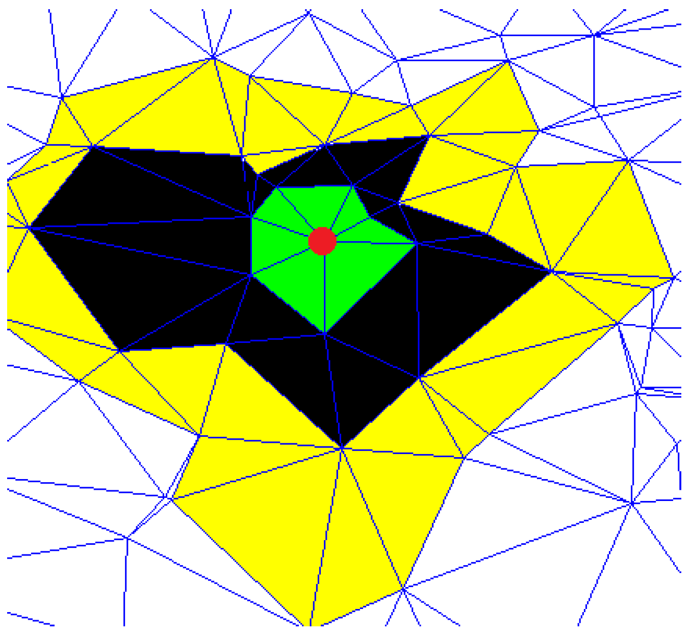
where each element of a generic column describes the involvement of a given node with its triangular pattern neighbors. Figure 1 shows an example of a node neighborhood. The red point represents the node under analysis, the green triangles are built considering the first-order proximity neighbors ($p=1$), the black triangles are built considering the second-order proximity neighbors ($p=2$), and the yellow ones are built considering the third order proximity neighbors ($p=3$). The application of this measure is linked to some fundamental aspects. First, the CCs are connected to other properties such as transitivity, density, characteristic path length, and efficiency. Transitivity verifies the number of passages of edges for a given node, while density provides information of centrality for a given subgraph or node. These centrality measures emphasize important nodes, especially in networks which present agglomerations in particular areas. Thus, CCs inherently capture further properties, enriching information to include in the features vector. Furthermore, the methods, exploring the graph in depth, adds another level of detail as it verifies the presence of structure in a wider area than the single neighborhood. This aspect is fundamental as the goal of embedding is to make sure that if two nodes are close in the graph, then they will be close in the embedding space. For this purpose, DOPSIE guarantees that nodes of a certain importance and spatial neighbors will present high values with respect to isolated nodes.

3.3. Our Algorithm

The proposed method takes as input a graph structure and encodes a vector representation for each node. As explained in the previous sections, the method explores an ever-growing neighborhood for every node in the network. This approach is dictated by the fact that topological information is not concentrated only in the nearest neighborhood but at a different distance. In fact, the goal is to represent not single nodes but particular areas in which the nodes are involved. Features about area are much richer and representative than punctual features. Furthermore, we have observed that the triangular pattern, taken into account, is the minimum closed polygon that includes three nodes and the simplest to detect providing a gain in terms of computational complexity. Algorithm 1 summarizes the steps of our method. The input parameters are the graph G and the node-order proximity dimension p.

Algorithm 1 DOPSIE algorithm

1: procedureGraph Embedding(G, p) 2:     $d\leftarrow 1$ 3:     for $i\leftarrow 1,\left|G\right|$ do 4:         ${CC}_i\left(G\right)\leftarrow \frac{{\delta }_i\left(G\right)}{k_i(k_i-1)}$ 5:         $ne\left(v_i\right)\leftarrow {CC}_i\left(G\right)$ 6:         $GE[i,d]\leftarrow ne\left(v_i\right)$ 7:     end for 8:     $d:=d+1$ 9:     for $i\leftarrow 1,\left|G\right|$ do 10:         $nn=FIND(G,v_i)$ 11:         $N\left(i\right)\leftarrow nn$ 12:         if $\left|nn\right|>0$ then 13:            $n{e}_{d-1}\left(v_i\right)\leftarrow {\sum }_{j=1}^{\left|nn\right|}{CC}_j\left(G\right)$ 14:            $GE[i,d]\leftarrow n{e}_{d-1}\left(v_i\right)$ 15:         else 16:            $GE[i,d]\leftarrow 0$ 17:         end if 18:     end for 19:     while $d\le (p+1)$ do 20:         $d:=d+1$ 21:         for $k\leftarrow 1,\left|N\right|$ do 22:            $NN\left(k\right)\leftarrow \varnothing$ 23:            $temp\leftarrow 0$ 24:            if $\left|N\right(k\left)\right|>0$ then 25:                for $j\leftarrow 1,\left|N\right(k\left)\right|$ do 26:                    $nnt=FIND(G,N(k).v(j\left)\right)$ 27:                    if $\left|nnt\right|>0$ then 28:                        $NN\left(k\right)\leftarrow NN\left(k\right)\cup nnt$ 29:                        $n{e}_{d-1}\left(v_k\right):=n{e}_{d-1}\left(v_k\right)+{\sum }_{z=1}^{\left|nnt\right|}{CC}_z\left(G\right)$ 30:                    end if 31:                end for 32:                $GE[k,d]\leftarrow n{e}_{d-1}\left(v_k\right)$ 33:            else 34:                $GE[k,d]\leftarrow 0$ 35:                $NN\left(k\right)\leftarrow \varnothing$ 36:            end if 37:         end for 38:         $N\leftarrow NN$ 39:     end while return$GE$ 40: end procedure

The CCs computed employing Equation (2) are stored in the first column of $GE$ matrix (Lines 3–7). After that, for each node, its neighbors of first order are exploited to compute the sum of their CCs (Lines 9–18).

Subsequently, from Lines 19–39 a depth exploration of the neighborhoods of each node with respect to the p input parameter is performed. It is the heart of the algorithm. At each step, the method explores a next level of depth in the graph with a limit equal to $p+1$ (line 20). For each depth level, it checks if there are nodes in the neighbors and store neighborhood information through the CCs measure (line 29). This exploration can be compared to the diffusion of a liquid that expands from a precise starting point (lines 21–38) and as shown in Figure 1. The starting point is the red node while the different colors represent the neighborhood levels explored during the iterations.

Finally, the algorithm returns $GE$. This matrix is composed of $\left|G\right|$·$(p+1)$ elements, where each row contains the embedding values encoding the nodes of the input graph.

Algorithm 2 Find the neighborhoods of the graph nodes

1: procedureFind(G,$v_i$) 2:     for $j\leftarrow 1,\left|G\right|$ do 3:         if ($e_i,e_j)=1$ then 4:            $nn\leftarrow nn\cup v_j$ 5:         end if 6:     end for return$nn$ 7: end procedure

3.4. Computational Complexity

In the following lines, we will analyze the time complexity of the main parts of DOPSIE.

• The CC computation (lines 3–7). The time complexity is $O\left(\right|G\left|\right)$. It is related to the number of graph nodes $\left|G\right|$.
• The research of the first order neighbors and the computation of the sum of the CCs of the neighbors (lines 9–18). The time complexity is $O\left(\right|G\left|\right)$.
• The exploration in depth of the nodes’ neighborhoods (lines 19–39). The time complexity is $O\left(\right|N\left(k\right)|·|N|·p)$, where $\left|N\right|$ is the number of the neighborhoods of all the nodes of a given order proximity dimension, $\left|N\right(k\left)\right|$ is the number of neighborhoods of a generic (k) node and p is the order proximity dimension value.

4. Results

In this section, we present the datasets and the experimental framework adopted to assess the quality of DOPSIE. We address different multilabel/multiclass classification problems through one-vs-all paradigm. The main task is divided into multiple binary tasks and the results obtained are expressed in terms of averaged accuracy.

4.1. Datasets

We have employed the following datasets:

• BlogCatalog [34], a network of social relationships provided by blogger authors. The labels represent the topic categories provided by the authors.
• Email-Eu-core [35], a network generated using email data from a large European research institution. We have an edge $(u,v)$ in the network if the person u sent to the person v at least one email. The dataset also contains “ground-truth” community memberships of the nodes. Each individual belongs to exactly one of 42 departments at the research institute.
• Wikipedia [36], a network of web pages. Labels represent the categories of web pages.

Table 1. Graphs adopted in our experiments.

Name	BlogCatalog	Email-Eu-core	Wikipedia
$\mid V\mid$	10312	1005	2405
$\mid E\mid$	667966	25571	17981
$\mid y\mid$	39	42	17

summarizes the overall details related to the employed datasets.

4.2. Experimental Framework

We have compared the classification performance achieved using the feature vectors computed by DOPSIE with those obtained by employing the following state-of-the-art graph-embedding algorithms: DeepWalk (DW) [20]; Graph Factorization (GF, [23]); HOPE, [22]; Node2vec [21].

Given an embedded dataset, the classification phase is performed by the Regularized Logistic Regression (RLR) [37] appropriately tuned. Moreover, distance proximity p is set to 10. This value is fundamental for the characterization of the network to be represented. After a training phase, a value equal to 10 is chosen. A low value ensures poor detail and computational optimization. By contrast, a high value enables an unrepresentative deep exploration of the neighborhood with an expensive computation. The datasets adopted are split into training and test sets. The training set are used to train the RLR classifier. An increasing percentage of data are adopted to understand the response in condition of variation. This phase is fundamental because it affects the quality of the classification model. The test set provides the standard approach to evaluate the model. It is only adopted once the model is completely trained. The test set contains carefully sampled data spanning the different classes that the model is composed of in the real world. We have chosen two performance measures. Accuracy gives an overall measure by checking only if the prediction of classifier is correct or wrong. Meanwhile, f-measure is more accurate as, in addition, it verifies the class of belonging of individual nodes of the network.

4.2.1. BlogCatalog

In this experiment we have randomly sampled a portion (from 10 to 90%) of the labeled nodes to create the training and test sets and we have repeated 10 times the process to average the results. All the hyper-parameters have been tuned by means of grid search. Please note that this dataset (formalized in Table 1) is strongly connected, and it is the bigger one considering of both the number of nodes and the number of edges.

Accuracy results are shown in

Table 2. Accuracy results achieved on BlogCatalog dataset. Results in bold represent the highest performance achieved for each column.

Per Train	DOPSIE	GF	HOPE	DW	Node2vec
10%	97.16	96.37	96.37	96.54	96.58
20%	97.24	96.38	96.37	96.56	96.61
30%	97.28	96.38	96.38	96.57	96.62
40%	97.29	97.17	97.11	97.15	97.21
50%	97.40	97.07	97.18	97.02	97.21
60%	96.01	95.77	95.30	95.32	95.05
70%	96.12	96.01	96.08	97.06	96.03
80%	96.72	96.09	96.05	96.43	96.24
90%	96.00	95.12	95.12	95.43	95.42

. Numbers in bold represent the highest performance achieved for each column. We can notice that DOPSIE consistently outperforms the other approaches. In contrast to the standard case, with the increase of the trained percentage, a proportional growth of the performance is not obtained. This behavior is linked to the nodes included for the test set, which presents several heterogeneous connections, which results in a description of the features vector, greatly affecting the performance.

F-measure results are shown in

Table 3. F-measure results achieved on BlogCatalog dataset. Results in bold represent the highest performance achieved for each column.

Per Train	DOPSIE	GF	HOPE	DW	Node2vec
10%	98.44	97.64	97.64	97.72	97.74
20%	98.46	97.64	97.64	97.73	97.76
30%	98.49	97.64	97.65	97.74	97.77
40%	98.49	98.34	98.15	98.14	98.01
50%	98.50	98.04	98.05	98.14	97.24
60%	97.72	97.22	97.21	97.12	97.64
70%	97.44	97.11	97.22	97.17	97.42
80%	97.46	97.01	97.28	97.16	97.26
90%	97.22	97.02	97.11	97.15	97.04

. Numbers in bold represent the highest performance achieved for each column. From this further experiment, we have the same indications. Clearly, the numerical results are slightly different because the f-measure is more sensitive to false positives and false negatives.

4.2.2. Email-Eu-core

In this experiment, we have randomly sampled a portion (from 10 to 90%) of the labeled nodes to create the training and test sets and we have repeated 10 times the process to average the results. All the hyper-parameters have been tuned by means of grid search.

This dataset has a lower number of nodes compared to the others. Moreover, it is important to notice that this dataset is particularly dense. Considering these peculiarities, the achieved accuracy results summarized in

Table 4. Accuracy results achieved on email-Eu-core dataset. Results in bold represent the highest performance achieved for each column.

Per Train	DOPSIE	GF	HOPE	DW	Node2vec
10%	95.81	97.61	97.62	97.45	97.24
20%	96.26	97.69	97.63	97.56	96.23
30%	97.19	95.67	95.68	94.65	93.64
40%	97.38	96.68	95.70	94.75	95.64
50%	97.47	94.67	95.71	95.74	94.64
60%	97.17	94.47	95.47	96.47	95.47
70%	97.74	96.47	96.37	96.44	96.44
80%	97.43	95.11	94.12	96.23	96.44
90%	97.44	96.33	96.21	96.12	96.44

show that DOPSIE outperforms Node2vec, GF and DW when dealing with big/medium training sets (30-40-50-60-70-80-90% of the labeled nodes). Otherwise, the performance of HOPE and GF are slightly better.

F-measure results are shown in

Table 5. F-measure results achieved on email-Eu-core dataset. Results in bold represent the highest performance achieved for each column.

Per Train	DOPSIE	GF	HOPE	DW	Node2vec
10%	98.77	98.80	98.80	98.67	98.79
20%	98.37	98.80	98.80	98.74	98.79
30%	98.56	97.80	97.81	97.80	97.80
40%	98.66	97.81	97.82	97.83	97.79
50%	98.69	97.80	97.82	97.83	97.79
60%	98.21	97.22	97.66	97.54	97.21
70%	98.11	97.32	97.47	97.23	97.24
80%	98.12	97.22	97.73	97.39	97.37
90%	98.62	97.35	97.11	97.96	97.91

. Numbers in bold represent the highest performance achieved for each column. The results obtained with f-measure are slightly different from the values obtained with accuracy. However, even in this case we get the same trend.

4.2.3. Wikipedia

In this experiment we have randomly sampled a portion (from 10 to 90%) of the labeled nodes to create the training and test sets and we have repeated 10 times the process to average the results. All the hyper-parameters have been tuned by means of grid search.

Accuracy results are summarized in

Table 6. Accuracy results achieved on Wikipedia dataset. Results in bold represent the highest performance achieved for each column.

Per Train	DOPSIE	GF	HOPE	DW	Node2vec
10%	93.67	92.13	92.13	92.79	92.83
20%	94.66	94.13	94.13	94.23	94.08
30%	94.11	93.13	93.13	93.40	93.21
40%	94.46	94.04	94.25	94.33	94.32
50%	94.19	93.14	93.17	93.59	93.42
60%	94.55	93.77	93.91	94.33	93.19
70%	94.32	93.13	93.17	93.54	93.32
80%	94.21	93.03	93.05	93.11	93.16
90%	94.56	93.53	93.32	93.21	93.00

. Numbers in bold represent the highest performance achieved for each column. This dataset presents fewer classes and is less dense than the other two. Nevertheless, also under this setting, DOPSIE shows better results with respect to those achieved by Node2vec, GF, HOPE, and DW.

F-measure results are summarized in

Table 7. F-measure results achieved on Wikipedia dataset. Results in bold represent the highest performance achieved for each column.

Per Train	DOPSIE	GF	HOPE	DW	Node2vec
10%	96.68	96.61	96.61	96.65	96.05
20%	96.83	96.91	96.91	96.91	96.85
30%	96.88	96.71	96.71	96.01	96.20
40%	96.92	96.91	96.21	96.02	96.55
50%	96.93	96.81	96.91	96.09	96.44
60%	96.21	96.12	96.02	96.11	96.11
70%	96.20	96.02	96.12	96.11	96.12
80%	96.18	96.02	96.11	96.07	96.12
90%	96.31	96.22	96.06	96.21	96.23

. Numbers in bold represent the highest performance achieved for each column. The results are numerically different but with the same trend, except for the case of 20% of training in which flattened values of 3 methods (GF, HOPE, DW) are presented.

5. Conclusions

In this work, we have proposed DOPSIE, a novel graph-embedding algorithm. Our method learns a representation that captures structural properties of the analyzed graph. We have proposed a wide experimental phase to demonstrate the effectiveness of our approach on multilabel and multiclass classification tasks. We have identified strong and weak points of the proposed approach. The main strong point consists of capturing structural features using exclusively the CC measure. The main weak point concerns the effort of capturing topological features when the network presents few connections, when nodes are poorly connected to each other. These nodes are considered not very representative, in terms of incoming and outgoing connections, and weakly characterize the graph. This aspect is reflected in a heterogeneous performance trend, as the current training set increases. The main challenge is to understand how to address this issue to make the method very distinctive in the context of network evaluation.

Possible future works might consist of exploring different concepts of proximity to further enrich the embedding features to improve the performance.