Article

Determination of the Steady State Fiber Orientation Tensor States in Homogeneous Flows with Newton–Raphson Iteration Using Exact Jacobians

by
Aigbe E. Awenlimobor
and
Douglas E. Smith
*
Department of Mechanical Engineering, Baylor University, Waco, TX 76706, USA
*
Author to whom correspondence should be addressed.
J. Compos. Sci. 2025, 9(8), 433; https://doi.org/10.3390/jcs9080433
Submission received: 6 July 2025 / Revised: 31 July 2025 / Accepted: 7 August 2025 / Published: 9 August 2025
(This article belongs to the Special Issue Theoretical and Computational Investigation on Composite Materials)

Abstract

Fiber orientation is an important descriptor of the microstructure for short fiber polymer composite materials where accurate and efficient prediction of the orientation state is crucial when evaluating the bulk thermo-mechanical response of the material. Macroscopic fiber orientation models employ the moment-tensor form in representing the fiber orientation state, and they all require a closure approximation for the higher-order orientation tensors. In addition, various models have more recently been developed to account for rotary diffusion due to fiber-fiber and fiber-matrix interactions which can now more accurately simulate the experimentally observed slow fiber kinematics in polymer composite processing. It is common to use explicit numerical initial value problem-ordinary differential equation (IVP-ODE) solvers such as the 4th- and 5th-order Dormand Prince Runge–Kutta (RK45) method to predict the transient and steady-state fiber orientation response. Here, we propose a computationally efficient method based on the Newton-Raphson (NR) iterative technique for determining steady state orientation tensor values by evaluating exact derivatives of the moment-tensor evolution equation with respect to the independent components of the orientation tensor. We consider various existing macroscopic-fiber orientation models and several closure approximations to ensure the robustness and reliability of the method. The performance and stability of the approach for obtaining physical solutions in various homogeneous flow fields is demonstrated through several examples. Validation of our orientation tensor exact derivatives is performed by benchmarking with results of finite difference techniques. Overall, our results show that the proposed NR method accurately predicts the steady state orientation for all tensor models, closure approximations and flow types considered in this paper and was relatively faster compared to the RK45 method. The NR convergence and stability behavior was seen to be sensitive to the initial orientation tensor guess value, the fiber orientation tensor model type and complexity, the flow type and extension to shear rate ratio.

1. Introduction

Characterization and evaluation of fiber suspensions has received considerable attention over the past four decades, particularly in the area of short fiber polymer composites produced in flow processes such as extrusion and molding. Understanding the motion and orientation of suspended fibers is critical for predicting the thermal, mechanical, and electrical performance of products made of these materials. Fiber orientation within a fiber suspension is often simulated using fiber orientation tensors, which provide a metric for assessing the random nature of sets of fibers and the degree of alignment. The goal of this paper is to compute the steady state orientation tensor of a fiber suspension in a homogeneous flow field using a Newton-Raphson iteration method with exact Jacobians.
Common tensor-based models used to compute the fiber orientation of a fiber suspension in polymer composite flows originated in the pioneering work by Jeffery [1], which described the evolution of a single rigid ellipsoid in a purely viscous flow of a Newtonian fluid. Jeffery’s hydrodynamic (HD) single ellipsoid model is limited to dilute suspension and ignores the effect of momentum diffusion due to fiber-fiber interactions. Moreover, Jeffery’s assumption ignores the flexural and fracture behavior of the fiber and assumes no slip contact between the fiber and surrounding fluid. Studies have shown that fibers suspended in industrial polymer melt flows tend to orient relative to the flow field [2], which is not captured in Jeffery’s work. As a result, enhancements to Jeffery’s single-fiber model have been made to better capture the bulk behavior of fibers in semi-dilute and concentrated suspension which include fiber-fiber interaction.
Although theoretically feasible, it is computationally expensive and nearly impractical to simulate the behavior of every individual particle in an industrially relevant short fiber polymer suspension flow. Alternatively, Folgar and Tucker [3,4] introduced isotropic rotary diffusion (IRD) and an orientation probability distribution function (ODF) to model interacting fiber suspensions based on Jeffery’s single-fiber model. The time evolution of the ODF is defined by the Fokker-Plank equation for probability distribution function (PDF) of fiber orientation. Conventionally, a numerical method such as finite volume (cf. Bay [5]) and, more recently, a more computationally efficient exact spherical harmonics method (cf. Montgomery-Smith et al. [6]) has been used to solve the Folgar-Tuckers (FT) equation of change for fiber orientation, but these methods have yet to see significant application in molding or extrusion processes. Advani and Tucker [7] proposed a tensorial representation of fiber orientation evolution based on the series expansion of even order moments of the ODF. Their approach simplifies computations, which has led to the widespread use of orientation tensors as the preferred method of evaluating fiber orientation for short fiber polymer composites. The Advani-Tucker (AT) orientation evolution model is commonly used to compute the 2nd order orientation tensor a i j , which requires a closure approximation of the 4th order orientation tensor a i j k l . Due to experimentally observed disparity in the fiber orientation kinematics compared to those computed from the Advani and Tucker orientation model [7], more recent modifications have been proposed in an effort to reduce the rate of alignment in polymer melt flow. Huynh [8] applied a strain reduction factor (SRF) to slow the transient response of the orientation tensor, which unfortunately lacked material objectivity. Alternatively, Wang et al. [9] introduced a phenomenological reduced strain closure (RSC) model that applies the reduction factor solely to the spectral decomposed principal rates of the orientation tensor without modifying effecting the rotation tensor, thus maintaining material objectivity. Similarly, Tseng et al. [10,11] proposed a retarding principal rate (RPR) model that involved a coaxial correction to the FT model by assuming the intrinsic orientation kinetics (IOK) describing the behavior of the fiber suspension involved a nonlinear modification to the principal directions of the material derivative.
Prediction of fiber orientation with IRD-based models has been validated experimentally for short-fiber/thermoplastic composites (SFT) with a fiber length typically in the range of 0.2 mm to 0.4 mm [12]. However, for long-fiber/thermoplastic composites (LFT) (e.g., with fiber lengths above 10 mm), IRD models tend to be less accurate with decreased alignment. Modifications to the rotary diffusion term have been proposed for improving accuracy when predicting the components of the orientation tensor. Ranganathan et al. [13] assumed an isotropic rotary diffusivity that inversely varies with the degree of alignment of the orientation tensor which was implemented using a phenomenological interaction parameter that depends on the reciprocal of the inter fiber spacing. The applicability of their model is limited to the transient orientation state while being well suited for long-range fiber-fiber interaction. Unfortunately, their model is known to be unsuitable for LFT steady state orientation prediction as with other IRD models, likely due to its isotropic diffusivity.
Fan et al. [14] and Phan-Thien [15] were the first to propose an anisotropic rotary diffusion (ARD) moment-tensor model by replacing the FT scalar phenomenological interaction parameter with a second order anisotropic rotary diffusion tensor. In a similar manner, Koch [16] developed an ARD model suited for semi-dilute suspensions with an anisotropic spatial diffusion tensor that depends on the orientation state and the rate of deformation tensor. However, their model was based on the more complicated PDF form for the orientation tensor representation rather than the moment-tensor form and proved ineffective in LFT modelling. Phelps and Tucker [12] extended the work of Fan [14] and Phan-Thien et al. [15] by developing a more general moment-tensor anisotropic diffusion model that depends on the spatial diffusion and orientation tensors called the Phelps-Tucker (PT) model. The derivation of the spatial diffusion tensor was written as a function of the orientation state and rate of deformation tensor in a similar manner to that proposed by Hand [17]. Phelps’s model showed remarkable improvements in predicting orientation states of LFTs. Tseng et al. [18] proposed the improved anisotropic rotary diffusion model (iARD) which defines a two-parameter spatial diffusion tensor that couples the effect of fiber-matrix interaction and fiber-fiber interaction. Unfortunately, the iARD model lacked material objectivity, limiting its applicability. More recently, Tseng et al. [19] proposed the principal anisotropic rotary diffusion (pARD) model assuming a principal spatial diffusion tensor that corotates with the orientation tensor. Bakharev [20] proposed the moldflow anisotropic rotational diffusion (mARD) model based on a reduction of the terms from the generic ARD model by Phelps to linear terms only with a spatial diffusion tensor like Tseng’s model. Latz et al. [21] developed a fully coupled flow-orientation model for concentrated suspensions by replacing the diffusion term in the FT model with an effective collision tensor that incorporates both and isotropic diffusion interaction term and a topological exclusion interaction term based on a nematic ‘Onsager’ potential of non-Brownian Maier-Saupe form (NEM-MS). They found the influence of the topological interaction on the fiber orientation state to be flow dependent, having a significant effect on channel and contraction flows, and found a relatively lesser influence for flow around cylinders. Kugler et al. [22], Favaloro et al. [23], Agboola et al. [24] and Park and Park [25] present detailed review and comparison of existing fiber orientation models. The foregoing ARD models are applied in polymer composite industry and have been incorporated in mold-filling flow computations in injection molding process simulations [26,27,28,29,30,31,32].
All fiber orientation tensor evolution equations include a tensor of higher order that must be evaluated or approximated. The common approach is to introduce a closure approximation that defines a higher-order fiber orientation tensor as a function of lower order information. Closure approximations are either based on an analytical expression or formed through a curve fitting process. The non-fitted analytical closure approximations include the those constructed from combinations of lower-order orientation and tensors and include the linear (LIN), quadratic (QDR), and the hybrid (HYB) closures. The general class of Hinch and Leal’s [33] composite closure approximations precontracted with the deformation rate tensor also falls under this category. Fitted closures are derived in terms of independent constants which are obtained using test data from solutions to the PDF for multiple standard flow conditions. The fitted closures include Eigenvalue-Based Fitted (EBF) and Invariant-Based Fitted (IBF) closures [34,35,36,37]. Higher-order optimal fitted closures such as the Eigenvalue-Based Optimal Fitted (EBOF) and Invariant-Based Optimal Fitted (IBOF) closures [34,35,36,37], which are extensions to the EBF and IBF closures, respectively, have also been developed for improved model accuracy. More details on different closure approximations and their associated advantages and disadvantages is discussed in later sections and also in [22,38,39,40]. Other fitted closure approximations include the neural network (NN)-based closures by Jack et al. [41,42] and the 6th-order Invariant-based orthotropic fitted closure by Jack and Smith [37,43].
The steady state values of orientation tensors in homogeneous flows have traditionally been computed with time evolution numerical IVP-ODE techniques such as the 4th-order Runge–Kutta method or predictor-corrector methods (see, e.g., [7,40]). However, when the objective is to obtain a steady-state orientation state, the transient solution process can require excessive computations for orientation tensor solution that are not needed. The main objective of this article is to present a computationally efficient approach for determining the steady state orientation tensors of fiber suspension in Newtonian homogenous flow field based on Newton-Raphson iteration with exact Jacobians. This approach zeros the time derivative of the 2nd order orientation tensor using explicit derivatives of the 2nd order orientation tensor rate of change equation with respect to its 2nd order orientation tensor components. Here, we consider various fiber orientation models and closure approximations and compare their performance in homogeneous flow fields. We benchmark the results of the explicit derivatives with those obtained using finite differences to ensure accuracy, and our Newton-Raphson iteration results are compared with time evolution numerical solutions in terms of both accuracy and efficiency. With the growing application of short carbon fiber-reinforced polymer composites in the additive manufacturing industry, the development of reliable and computationally efficient modelling tools for modelling fiber suspension in order to better understand the development of the inherent bead microstructure is crucial. Our NR technique can be incorporated into existing commercially available short fiber orientation modelling software as a viable alternative to conventional numerical IVP-ODE techniques for determining the fiber orientation steady state which can improve the overall computational performance.

2. Materials and Methods

2.1. Representation of Fiber Orientation State

Figure 1 shows an orientation state of a prolate ellipsoid including the local coordinate systems x 1 , x 2 , x 3 and Euler angles definition where the orientation vector p _ lies along the major axis of the ellipsoid.
The orientation state of a fiber, as shown in Figure 1, can be described by the unit vector p _ as follows [7]:
p _ = sin θ cos ϕ sin θ sin ϕ cos θ T
The orientation of the unit vector p _ is commonly described in terms of the probability distribution function (PDF) ψ p _ over all possible directions of p _ . It can be shown that ψ p _ = ψ p _ satisfies the normalization condition.
ψ p _ d p _ = θ = 0 π ϕ = 0 2 π ψ θ , ϕ sin θ   d θ d ϕ = 1
The PDF ψ p _ also satisfies the continuity condition [7].
D ψ D t = p _ ψ p _ ˙
A set of higher-order, even order tensors, can also be used to describe the orientation state of a single fiber or fiber suspension such as the 2nd and 4th-order orientation tensors, given, respectively, as
a i j = p i p j ψ p _ d p _ a n d a i j k l = p i p j p k p l ψ p _ d p _
Orientation tensors in Equation (4) are completely symmetric, i.e.,
a i j = a j i a i j k l = a j i k l = a k i j l = a l i j k = a i k j l = a i l j k =         , 24   p e r m u t a t i o n s
and a normalization condition requires that
a i i = 1 , a i j k k = a i j
Consequently, there are only 5 independent components in a i j and 9 independent components in a i j k l .

2.2. Determination of Steady State Orientations

The numerical approach developed here for determining steady state values of the orientation vector p i and orientation tensor components a i j computes a zero rate of change of each corresponding evolution equation using the Newton-Raphson method. The rate of change equation (often referred to as the residual, R i ) for both p i and a i j are set to zero, respectively:
R i = D p i D t = 0 a n d R i j = D a i j D t = 0
where i , j 1,2 , 3 , and summation convention is implied unless otherwise stated. Newton-Raphson iteration computes the root (in our case the orientation state) as [44]
p i + = p i [ J i j ( p i ) ] 1 R j ( p i )
for the orientation vector and
a i j + = a i j [ J m n i j a i j ] 1 R m n a i j
for the 2nd order orientation tensor, where the ( + ) and ( ) superscripts denote the current and previous iteration, respectively. The implication of Equations (8) and (9) is the need to compute the Jacobians J i j and J m n i j , which are the derivatives of the orientation vector and tensor, respectively, with respect to its components that define them, i.e.,
J i j = R i p j a n d J m n i j = R m n a i j
The above computations, including the 2nd and 4th order tensor inverse calculations, are conveniently performed using contracted tensor notation. Since there are only 5 independent components of a i j (see discussion below), the residual R m n may be represented in contracted form as the vector R r (and similarly, the tensor a i j may be represented as the vector a r ), and the Jacobian J m n i j as a matrix J r s . The contracted notation is related to the tensor components through index mapping.
r m , n = n 1 2 m 1 m 6 , f o r   n = m 3 , f o r   m = 1 , 2
It follows that Equation (9) in contracted notation becomes
a r + = a r [ J r s ( a r ) ] 1 R r ( a r )
In the following sections, we present existing models for rate of change equations of the orientation vector p i and tensor a i j based on those considered in the review by Kugler et al. [22]. Equating each rate of change equation to zero yields the Newton-Raphson residual in Equation (1), which is then differentiated to obtain expressions for the associated Jacobian.

2.3. Fiber Orientation Modelling in the Dilute Regime

Jeffery’s hydrodynamic model for the motion of a single rigid ellipsoidal particle in an incompressible Newtonian viscous fluid flow field forms the basis for evaluating fiber orientation for dilute suspensions. (Dilute suspension is a heterogenous suspension where the average interparticle spacing is relatively large such that there is no restriction on the fibers motion due to hydrodynamic forces or mechanical contact. More details on fiber suspension concentration regimes can be found in [45,46].) Jeffery assumed that an ellipsoidal particle is convected with the bulk motion of the undisturbed surrounding fluid where the rate of change of p _ written in component form is given as [1,22,23]
p ˙ i = ω i j p j + ξ γ ˙ i j p j γ ˙ k l p k p l p i
where ω i j and γ ˙ i j are the anti-symmetric and symmetric decomposition of the rate of deformation tensor L i j , given as
ω i j = 1 2 v i x j v j x i a n d γ ˙ i j = 1 2 v i x j + v j x i
such that L i j = v i / x j = γ ˙ i j + ω i j , and ξ is a particle shape parameter given as ξ = r e 2 1 / r e 2 + 1 for a particle with equivalent ellipsoidal aspect ratio r e . It is worth noting that r e can be related to the geometric aspect ratio of various axisymmetric particle shapes such as cylindrical particles [47]. We define components R i of the Newton-Raphson residual in Equation (8) for computing the steady-state orientation of the vector p _ in Equation (9) as
R i J F = p ˙ i
where the superscript J F denotes the ‘Jeffery’ type residual. The Jacobian J m n J F = R m J F p n is obtained by taking derivatives of the components R m J F with respect to p n , i.e.,
J m n J F = p ˙ m p n = ω m j δ j n + ξ γ ˙ m j δ j n γ ˙ k l δ k n p l p m + p k δ l n p m + p k p l δ m n
where we note that derivatives of p _ , with respect to itself, form the identity tensor., i.e., p i / p j = δ i j . Equation (16) contains only 2 independent components of the orientation vector R i J F , making it possible to represent the components of J m n J F as a 2 × 2 matrix. Although Jeffery’s model for dilute suspensions has limited direct application since fiber-fiber interaction is ignored, the NR method can be used to find the steady state solution for flows with a high extension to shear rate ratio, such as those considered in [48].

2.4. Fiber Orientation Modelling in Semi-Dilute and Concentrated Regime

In the concentrated regime, the average interparticle spacing is very small (orders of magnitude less than the smallest particle dimension) such that the fiber motion is affected by hydrodynamic forces and possible direct mechanical contact with other particles. Definitions for the semi-dilute and concentrated fiber suspension regimes can be found in [45,46]. The effect of the interparticle interaction on the single particle’s motion is typically modeled by including a momentum diffusion term in Equation (13). Here, we consider various diffusion models which are commonly used in commercial SFRP simulations having fiber suspensions in the concentrated regime. In the following sections, the NR method for resolving the steady state fiber orientation is developed for multiple 2nd order fiber orientation tensor and rotary diffusion models and include several 4th order closure approximations.

2.4.1. The Folgar-Tucker Diffusion Model

A model that accounts for the effect of momentum diffusion due to short- and long-range fiber-fiber interaction in non-dilute fiber suspensions was first proposed by Folgar-Tucker model [3,4] by incorporating a rotary diffusion term into Jeffery’s single fiber model as
p ˙ i F T = p ˙ i J F D r 1 ψ ψ p i
where D r is the rotary diffusivity constant that introduces a Brownian diffusion effect among contacting particles. For long slender particles (i.e., ξ 1 ), Folgar and Tucker set D r = C I γ ˙ , where C I is a phenomenological interaction coefficient and γ ˙ = 2 γ ˙ i j γ ˙ j i is the scalar magnitude of the strain rate tensor γ ˙ i j . The orientation PDF ψ in Equation (17) defines the probability that a given fiber has a particular orientation (see [3,4,7]). Advani and Tucker [7] derived the orientation tensor form of the Folger-Tucker model defined in terms of the 2nd and 4th order orientation tensors. Advani and Tucker developed an equation for the rate of change of a i j , identified as the orientation material derivative tensor a ˙ i j in terms of the 2nd and 4th order tensor:
D a i j A T D t = a ˙ i j A T = a ˙ i j H D + a ˙ i j I R D
where a ˙ i j H D is the hydrodynamic component derived from Jeffery’s equation (cf. Equation (11)) given as
a ˙ i j H D = ω i k a k j a i k ω k j + ξ γ ˙ i k a k j a i k γ ˙ k j 2 γ ˙ k l a i j k l
and a ˙ m n I R D is the added isotropic rotary diffusion:
a ˙ i j I R D = 2 D r δ i j α a i j
In the above, α is a dimension factor (i.e., α = 3 for 3D orientation and α = 2 for 2D planar orientation). It follows that the residual in Equation (8) for the Advani-Tucker model is
R m n A T = a ˙ i j A T
The associated Jacobian J m n i j F T for the Advani-Tucker model is obtained by differentiating R m n A T with respect to the components of a i j , yielding
J m n i j A T = R m n A T a i j = a ˙ m n H D a i j + a ˙ m n I R D a i j
Given that the derivative of a i j with respect to itself is
a m n a i j = δ m i δ n j
the derivative terms on the right-hand side of Equation (22) may be written as
a ˙ m n H D a i j = ω m k + ξ γ ˙ m k δ k i δ n j + ω k n + ξ γ ˙ k n δ m i δ k j 2 ξ γ ˙ k l a m n k l a i j
a ˙ m n I R D a i j = 2 D r α δ m i δ n j
Expressions for derivatives of a m n k l (i.e., a m n k l a i j ) in Equation (24) and others using well known closure approximations are presented in the following sections.

2.4.2. Strain Reduction Factor (SRF) Model

The SRF model was developed by Huynh [8] to reduce the rate of alignment as compared to the AT model by introducing a strain reduction factor κ ( 0 < κ < 1 ) into Equation (16) (i.e., multiplying the right-hand-side of Equation (16) by κ ) to slow down the orientation kinetics as observed experimentally. He based his premise on a reduced bulk strain of fiber clusters in a concentrated suspension flow. The residual and Jacobian in this case is just a multiplication of κ with that previously obtained for the FT model.
R m n S R F = κ R m n A T , J m n i j F T = κ J m n i j A T , 0 < κ < 1
Steady state orientations predicted by the SRF model have been experimentally validated [9]; however, it tends to overshoot measured alignments in the initial transient. The SRF model also does not satisfy the rheological test of material objectivity and, therefore, cannot be applied to complex flows.

2.4.3. Reduced Strain Closure (RSC) Model

Wang et al. [9] addressed material objectivity with their reduced strain closure (RSC) model which applies a reduction factor only to the evolution rate of the spectral decomposed principal directions Φ _ _ of the orientation tensor λ ˙ _ , without modifying the rate of rotation Φ _ _ ˙ , given as
λ ˙ i R S C = κ λ ˙ i A T , Φ ˙ i j R S C = Φ ˙ i j A T , a m n | a m n = λ i Φ m i Φ n i
where | denotes the mathematical abbreviation for ‘such that’, and repeated indices imply summation. It follows that the material derivative for the RSC model may be written as [9]
a ˙ m n R S C = a ˙ m n A T 1 κ a ˙ m n Δ A T
where the kernel of a ˙ m n Δ A T defines the part of the standard AT model affected by the modification factor κ to yield the RSC model, given as
a ˙ m n Δ A T = λ ˙ i A T Φ m i Φ n i = 2 ξ γ ˙ k l L m n k l M m n r s a r s k l + a ˙ m n I R D
where
L m n k l = λ ˙ i Φ m i Φ n i Φ k i Φ l i , M m n k l = Φ m i Φ n i Φ k i Φ l i
The Newton-Raphson residual for the RSC model is R m n R S C = a ˙ m n R S C , and the Jacobian is obtained by taking partial derivatives of Equation (31) as follows:
J m n i j R S C = J m n i j F T 1 κ a ˙ m n Δ A T a i j
where
a ˙ m n Δ A T a i j = 2 ξ γ ˙ k l a i j L m n k l M m n r s a r s k l + a ˙ m n I R D a i j
which can be re-written as
a ˙ m n Δ A T a i j = 2 ξ γ ˙ k l L m n k l a i j a r s k l M m n r s a i j M m n r s a r s k l a i j + a ˙ m n I R D a i j
In the above, the derivatives of 4th order tensors M m n k l and L m n k l are obtained by differentiating Equation (33), respectively, as
M m n k l a r s = a r s Φ m i Φ n i Φ k i Φ l i = Φ n i Φ k i Φ l i Φ m i a r s + Φ m i Φ k i Φ l i Φ n i a r s + Φ m i Φ n i Φ l i Φ k i a r s + Φ m i Φ n i Φ k i Φ l i a r s
and
L m n k l a r s = Φ m i Φ n i Φ k i Φ l i λ ˙ i a r s + λ ˙ i a r s Φ m i Φ n i Φ k i Φ l i
where the derivatives of the eigenvalues λ i and eigenvectors Φ j k appearing in Appendix A have been used to simplify the final expression.

2.4.4. Retarding Principal Rate (RPR) Model

Tseng et al. [10,11] developed a Retarding Principal Rate (RPR) model, which, like the RSC model, reduces fiber orientation kinetics. Their approach is based on a coaxial modification to the principal directions of the orientation tensor evolution rate via a nonlinear correlation. The material derivative tensor a ˙ m n X of any standard model X (where X can define the AT, RSC, or other orientation tensor evolution model) is linearly combined with the RPR correction to slow down the orientation response rate, i.e.,
a ˙ m n X R P R = a ˙ m n X + a ˙ m n R P R
where the RPR correction a ˙ m n R P R is written in terms of its eigenvalue derivative matrix Λ ˙ k l I O K as
a ˙ m n R P R = Φ m k Λ ˙ k l I O K Φ n l , Λ ˙ k l I O K = Λ ˙ k l I O K λ ˙ _ X
where Λ ˙ k l I O K is the correction to the principal values of the orientation tensor material derivative based on the IOK assumption (see, e.g., Equation (41) below). The superscript on Λ ˙ k l I O K indicates the intrinsic orientation kinetics (IOK) assumption. Given that the correction is coaxial, the rotation tensor growth rate is unaffected and is obtained from the spectral decomposition of a m n , where Φ _ _ satisfies
Λ m n = Φ k m a k l Φ l n
The columns of the eigenmatrix obtained in this way are reordered in descending order with respect to the magnitude of the eigenvalues, i.e.,
Φ i j = Φ i j | λ j = Λ j j , λ 1 λ 2 λ 3
where | denotes the mathematical abbreviation for ‘such that’ and the repeated indices in Λ j j do not imply summation but rather represent the j t h diagonal component of Λ i j . The growth rate of the principal eigenvalues of the standard model X, i.e., Λ ˙ k l X , is obtained from
Λ ˙ k l X = Φ k m a ˙ k l X Φ l n , λ ˙ k X = Λ ˙ k k X
The diagonal tensor Λ ˙ k k I O K is defined by a 2-parameter non-linear correlation to the principal values of the standard model Λ ˙ k l X such that
Λ ˙ k k I O K = λ ˙ k I O K = α λ ˙ k X β λ ˙ k X 2 + 2 λ ˙ l X λ ˙ m X , Λ ˙ k l I O K k l = 0
For an RPR corrected model, the NR residual R m n X R P R is simply the material derivative
R m n X R P R = a ˙ m n X R P R
and the Jacobian J m n i j X R P R is given as
J m n i j X R P R = a ˙ m n X a i j + a ˙ m n R P R a i j
The partial derivative of the RPR correction term a ˙ m n R P R is
a ˙ m n R P R a i j = Φ m k a i j Λ ˙ k l I O K Φ n l + Φ m k Λ ˙ k l I O K a i j Φ n l + Φ m k Λ ˙ k l I O K Φ n l a i j
and the partial derivative of the modified growth rate of eigenvalues tensor Λ ˙ k l I O K is obtained by taking the derivative of Equation (41) as
Λ ˙ k k I O K a i j = λ ˙ k I O K a i j = α λ ˙ k X a i j 2 β λ ˙ k X λ ˙ k X a i j + λ ˙ l X a i j λ ˙ m X + λ ˙ l X λ ˙ m X a i j , Λ ˙ k l I O K a i j k l = 0
where
Λ ˙ k l X a i j = Φ k m a i j a ˙ k l X Φ l n + Φ k m a ˙ k l X a i j Φ l n + Φ k m a ˙ k l X Φ l n a i j , λ ˙ k X a i j = Λ ˙ k k X a i j
In the above, a ˙ m n X a i j is the partial derivative of material derivative a ˙ m n X with respect to the components of a i j obtained a priori, and the partial derivatives of the eigenvector matrix with respect to the same i . e . , Φ m n a i j can be obtained as shown in Appendix A (cf. [49]).

2.4.5. Anisotropic Rotary Diffusion (ARD) Models

While the IRD models were experimentally observed to be accurate in predicting the orientation state of short-fiber/thermoplastic composites (SFT), they were ineffective in accurately predicting the complete set of orientation tensor components for the long-fiber/thermoplastic composites (LFT), which motivated ARD model development. Various ARD models and modified forms have been developed based on the definition of the spatial diffusion tensor. Most models utilize the moment-tensor form for the ARD representation developed by Phelps and Tucker [12]. The general expression for the 2nd order orientation tensor evolution rate is a linear combination of the Jeffery’s-based model and the rotary diffusion term, given as
a ˙ m n P T = a ˙ m n H D + a ˙ m n A R D
where the rotary diffusion term a ˙ m n A R D is defined in terms of the spatial diffusion coefficient and the orientation state, given as
a ˙ m n A R D = γ ˙ 2 C m n 2 C r s δ r s a m n 5 C m k a k n + a m k C k n + 10 a m n k l C k l
and C _ _ is the spatial diffusion tensor. Based on this model, the NR residual and Jacobian are, respectively, given as
R m n P T = a ˙ m n P T
J m n i j P T = a ˙ m n P T a i j = a ˙ m n H D a i j + a ˙ m n A R D a i j
where the derivative of the rotary diffusion ( A R D ) term is obtained using product rule as follows:
a ˙ m n A R D a i j = γ ˙ [ 2 C m n a i j   2 C r s a i j δ r s a m n + C r s δ r s δ m i δ n j +   5 C m k a i j a k n + C m k δ k i δ n j + δ m i δ k j C k n + a m k C k n a i j + +   10 a m n k l a i j C k l + a m n k l C k l a i j ]
In the Mold-Flow ARD (mARD) model developed by Bakharev [20], the Phelps and Tucker’s rotary diffusion ARD expression is truncated to include just the linear terms, i.e.,
a ˙ m n m A R D = γ ˙ 2 C m n 2 C k l δ k l a m n
a ˙ m n m A R D a i j = γ ˙ 2 C m n a i j 2 C k l a i j δ k l a m n + C k l δ k l δ m i δ n j
The corresponding evolution rate equation for the 2nd order orientation tensor based on mARD model is given as
a ˙ m n m P T = a ˙ m n H D + a ˙ m n m A R D
Various forms of the spatial diffusion coefficient C m n used in the ARD model (indicated by a superscript in the following) have been developed. The Phelps and Tucker [12] representation C m n P T based on a modification to Hand’s anisotropic tensor [17] is given as a function of the rate of deformation tensor γ ˙ i j and orientation state a i j as
C m n P T = b 1 δ m n + b 2 a m n + b 3 a m k a n k + b 4 γ ˙ γ ˙ m n + b 5 γ ˙ 2 γ ˙ m k γ ˙ n k
where b i are dimensionless constants and are determined experimentally. The derivative of the C m n P T with respect to a i j that is substituted into Equation (56) is
C m n P T a i j = b 2 δ m i δ n j + b 3 δ m i δ k j a n k + a m k δ n i δ k j
The sensitivity of the numerical stability of the model response on the PT model parameters b i coupled with the complicated process involved in their determination are major limitations to the application of this model. Tseng et al. [18] developed an improved anisotropic rotary diffusion model (iARD) with a two-parameter spatial diffusion tensor representation written in terms of γ ˙ i j and its scalar magnitude γ ˙ that couples the effect of fiber-matrix interaction and fiber-fiber interaction, given as
C m n i A R D = C I δ m n 4 C M γ ˙ m k γ ˙ n k γ ˙ 2
where C I and C M are the fiber-fiber and fiber-matrix interaction parameters, respectively. An alternate form of Equation (60) is given as
C m n i A R D = C I δ m n C M L ~ m n , L ~ m n = L m k L n k / L r s L r s
where L m n is the rate of deformation tensor. The derivative C m n i A R D with respect to a i j is simply zero, i.e.,
C m n i A R D a i j = 0
Due to the lack of material objectivity of the rate of deformation tensor L m n , in Equation (61), Tseng et al. [19] developed an improved objective principal spatial tensor ARD model (pARD) that is coaxial with the orientation tensor, given as
C m n p A R D = C I Φ m k D k l Φ n l , Φ _ _ | a m n = Φ m k a ¯ k l Φ n l
where the tensor D k l contains only diagonal terms, and its trace is unity, i.e.,
D k k = 1 , D k l k l = 0
The derivative of C m n p A R D with respect to the 2nd order orientation tensor for substitution into Equation (56) is
C m n p A R D a i j = C I Φ m k a i j D k l Φ n l + Φ m k D k l Φ n l a i j
Another ARD model form suggested by Wang [50] called the Wang-Phelps-Tucker (WPT) model involved truncating the terms of the PT model to obtain
C m n W P T = b 1 δ m n + b 3 a m k a n k
Falvoro et al. [23] provided an alternative form of C m n W P T , where he replaced the coefficients in Equation (66) with a weighted superposition of the interaction coefficient C I , written as
C m n W P T = C I 1 w δ m n + w a m k a n k
where w is the weighting factor. The derivative of C m n p A R D with respect to a i j for substitution into Equation (56) is
C m n W P T a i j = w C I δ m k a n k + a m k δ n k
Lastly, we consider the D z ARD model (cf. Falvoro et al. [23]) developed by Moldflow for simulating 2.5 D flow processes. Their model is defined in terms of the interaction coefficient C I , a moment of interaction thickness parameter D z , and the unit normal to the mold surface n ^ . The expression for C m n for the D z ARD model is
C m n D z = C I D z δ m n 1 D z n ^ m n ^ n
and
C m n D z a i j = 0

2.4.6. Nematic Potential (NEM) Model

Latz et al. [21] proposed a 2-parameter nematic potential ARD (NEM) model that couples the phenomenological effect of the momentum diffusion due to fiber-fiber interaction and a topological interaction effect of diffusion due to an exclusion volume mechanism. The material derivative of the 2nd order orientation tensor based on the nematic diffusion model is
a ˙ m n n e m = a ˙ m n H D + a ˙ m n I R D M S
where
a ˙ m n I R D M S = γ ˙ C I δ m n α a m n + U 0 a m k a k n a k l a m n k l
In the above, U 0 is the ‘Onsager’ nematic topological interaction coefficient of the Maier-Saupe (MS) potential. Typically, for stability, U 0 4 C I for 2D analysis and U 0 > 8 C I for 3D analysis. The NR residual and Jacobian are, respectively, given as
R m n n e m = a ˙ m n n e m
J m n i j n e m = a ˙ m n H D a i j + a ˙ m n I R D M S a i j
where the derivative of the nematic diffusion term is obtained from Equation (72) as
a ˙ m n I R D M S a i j = γ ˙ C I α δ m i δ n j + U 0 δ m i δ k j a k n + a m k δ k i δ n j δ k i δ l j a m n k l a k l a m n k l a i j
It is common to combine multiple diffusion models when predicting the orientation state with the goal of improved accuracy. One such combination is the ARD-RSC models, whose material time derivative is expressed as [19]
a ˙ m n p A R D R S C = a ˙ m n R S C κ a ˙ m n I R D + a ˙ m n A R D + a ˙ m n Δ R S C
where
a ˙ m n Δ R S C = 2 γ ˙ 1 κ M m n k l δ k l a m n 5 L m n k l M m n r s a r s k l C k l
and a ˙ m n I R D , a ˙ m n R S C , and a ˙ m n A R D are given in Equations (20), (28) and (48), respectively. In this case the NR residual R m n p A R D R S C is the material derivative a ˙ m n p A R D R S C , i.e.,
R m n p A R D R S C = a ˙ m n p A R D R S C
and the Jacobian is obtained by taking the partial derivative of Equation (76) with respect to a i j as
J m n i j p A R D R S C = a ˙ m n R S C a i j κ a ˙ m n I R D a i j + a ˙ m n A R D a i j + a ˙ m n Δ R S C a i j
where
a ˙ m n Δ R S C a i j = 2 γ ˙ 1 κ M m n k l a i j δ k l δ m i δ n j 5 a i j L m n k l M m n r s a r s k l C k l + M m n k l δ k l a m n 5 L m n k l M m n r s a r s k l C k l a i j
The partial derivative terms on the right-hand side (R.H.S) of Equation (90) appear in the previous sections.

2.5. Closure Approximations and Their Explicit Derivatives

Derivatives of the orientation tensor closure approximation are used in the Newton-Raphson iteration method to compute the steady-state fiber orientation tensor state. The derivatives used in this study are described below.

2.5.1. Quadratic Closure Approximation

The quadratic (QDR) closure a ~ i j k l was introduced by Doi [51] and Lipscomb [52] and is defined as dyadic product of the 2nd order orientation tensor a i j :
a ~ i j k l = a i j a k l
The derivative of a ~ i j k l with respect to a m n is
a ~ i j k l a m n = a i j a m n a k l + a i j a k l a m n = δ i m δ j n a k l + a i j δ k m δ l n
The QDR closure inherently lacks symmetry but preserves the required symmetry of the computed a m n when employed in the Advani-Tucker equation (cf. Equation (18)).

2.5.2. Linear Closure Approximation

The linear (LIN) closure approximation of a ^ i j k l first proposed by Hand [17] uses all possible products of the 2nd order orientation tensor a i j and the identity tensor δ i j as follows:
a ^ i j k l = h 1 ( δ i j δ k l +   δ i k δ j l + δ i l δ j k ) +   h 2 a i j δ k l + a i k δ j l + a i l δ j k + δ i j a k l + δ i k a j l + δ i l a j k
where h 1 and h 2 are numerical factors which vary based on spatial dimensionality. h 1 = 1 / 35 for three-dimensional orientation and h 1 = 1 / 24 for planar orientation, while h 2 = 1 / 7 for three-dimensional orientation and h 2 = 1 / 6 for planar orientation [7]. It follows that the derivative of a ^ i j k l with respect to a m n is
a ^ i j k l a m n = h 2 δ i m δ j n δ k l + δ i m δ k n δ j l + δ i m δ l n δ j k + δ i m δ j n δ k l + δ i m δ k n δ j l + δ i m δ l n δ j k
The LIN closure is exact for random orientation distribution, while the QDR closures are exact for a uniaxially aligned fiber orientation.

2.5.3. Hybrid Closure Approximation

The hybrid closure approximation a i j k l is a weighted combination of the a ^ i j k l and a ~ i j k l defined above, written in terms of Herman’s Orientation factor (HOF), f , as follows [7]:
a i j k l = f a ~ i j k l + 1 f a ^ i j k l
Advani & Tucker [7] proposed an expression for f as an invariant of the orientation state given as f = a f a i j a j i b f , where a f and b f are constants that depend on the spatial dimension. a f = 3 / 2 for three-dimensional orientation and a f = 2 for planar orientation, while b f = 1 / 2 for three-dimensional orientation and b f = 1 for planar orientation.
The derivative of the hybrid closure approximation a i j k l with respect to components of the 2nd order tensor a m n is
a i j k l a m n = f a ~ i j k l a m n + 1 f a ^ i j k l a m n + f a m n a ~ i j k l a ^ i j k l
where
f a m n = a f δ i m δ j n a j i + a i j δ j m δ i n
We denote the hybrid closure based on this HOF form as HYB1. An alternative form of the HOF, f , proposed by Advani & Tucker [7], is
f = 1 α α e i j k a i 1 a j 2 a k 3
where it follows that
f a m n = α α e i j k δ i m δ 1 n a j 2 a k 3 + a i 1 δ j m δ 2 n a k 3 + a i 1 a j 2 δ k m δ 3 n
We denote hybrid closure based on this alternative form of the HOF as HYB2. The hybrid model is observed to perform better during the transient orientation prediction; however, the hybrid closure was shown to over-predict the steady state fiber alignment compared with simulation results based on the more accurate orientation distribution function, which are computationally expensive since they require a finite difference grid in space and time.

2.5.4. Hinch and Leal Closure Approximation

Hinch and Leal [33] developed numerous composite closure approximations for the 4th order orientation tensor in precontracted forms with the deformation rate tensor. The accuracy of their predictions was shown to depend on the flow field and flow magnitude considered. Hinch and Leal (HL) closure approximations are not explicit expressions of the 4th order orientation tensor a i j k l but are instead written in contracted form with the deformation rate tensor, i.e., γ k l a i j k l . Advani and Tucker provide a general explicit expression of a i j k l (cf. Equation (86)), summarizing all Hinch and Leal (HL) closures as
a i j k l = β 1 δ i j δ k l +   β 2 δ i k δ j l + δ i l δ j k + β 3 δ i j a k l + a i j δ k l +   β 4 a i k δ j l + a j l δ i k + a i l δ j k + a j k δ i l + β 5 a i j a k l + β 6 a i k a j l + a i l a j k +     +   β 7 δ i j a k m a m l + a i m a m j δ k l + β 8 a i m a m j a k n a n l
where β i are defined in Table 1. The partial derivative of the above expression with respect to a r s is
a i j k l a r s = [ β 1 a r s ( δ i j δ k l ) + β 2 a r s δ i k δ j l + δ i l δ j k + β 3 a r s δ i j a k l + a i j δ k l + β 4 a r s a i k δ j l + a j l δ i k + a i l δ j k + a j k δ i l +   β 5 a r s a i j a k l + β 6 a r s a i k a j l + a i l a j k + β 7 a r s δ i j a k m a m l + a i m a m j δ k l +   β 8 a r s a i m a m j a k n a n l ] +   [ β 3 δ i j δ k r δ l s + δ i r δ j s δ k l + β 4 δ i r δ k s δ j l + δ j r δ l s δ i k + δ i r δ l s δ j k + δ j r δ k s δ i l +   β 5 δ i r δ j s a k l + a i j δ k r δ l s + β 6 δ i r δ k s a j l + a i k δ j r δ l s + δ i r δ l s a j k + a i l δ j r δ k s +   β 7 δ i j δ k r δ m s a m l + δ i j a k m δ m r δ l s + δ i r δ m s a m j δ k l + a i m δ m r δ j s δ k l +   β 8 δ i r δ m s a m j a k n a n l + a i m δ m r δ j s a k n a n l + a i m a m j δ k r δ n s a n l + a i m a m j a k n δ n r δ l s ]
Mullens [40] provided a summary table (cf. Table 1) for the β i factors of the Hinch and Leal (HL) closures subdivided into weak flow (WF) (Isotropic (ISO), Linear (LIN) and Quadratic (QDR)) and strong flow (SF), and Hinch and Leal first composite (HL1) and second composite (HL2) closure forms.
Table 1. Summary of the Hinch and Leal closure β i factors for the different flow classifications.
β 1 β 2 β 3 β 4 β 5 β 6 β 7 β 8
WFISO 1 15 1 15
LIN 1 35 1 35 1 7 1 7
QDR 1
SFSF2 1 1 2 a 2
HLHL1 2 5 1 5 3 5 2 5
HL2 26 315 α 26 315 α 16 63 α 4 21 α 1 1 2 a 2
where the parameters a 2 and α are, respectively,
a 2 = a i j a j i , α = exp 2 1 3 a 2 1 a 2
and the partial derivatives are, respectively, given as
a 2 a r s = δ i r δ j s a j i + a i j δ j r δ i s α a r s = 4 α 1 a 2 2 a 2 a r s ,   a r s k a 2 = k a 2 2 a 2 a r s

2.5.5. Eigenvalue-Based Fitted (EBF) Closure Approximations

More recently, fitted closure approximations have emerged, including the Eigenvalue-Based Fitted (EBF) closures that require a principal axis transformation which ensures material objectivity. Orthotropic closure approximations for the 4th order tensor implicitly impose objectivity such that the approximation is independent of the coordinate frame selection. Indeed, the Orthotropic Linear (ORT), Orthotropic Smooth (ORS), Orthotropic Fitted (ORF) closures, ORF closure for low fiber-fiber interaction coefficient (ORL), ORF closure for wide range of fiber-fiber interaction coefficient values with 2nd order orientation tensor eigenvalue polynomial expansions (ORW), ORW closure with 3rd order orientation tensor eigenvalue polynomial expansions (ORW3), orthotropic natural closure—exact midpoint fit (NAT1) and orthotropic natural closure—and extended quadratic fit (NAT2) are included in the EBF family of closures originally developed by Cintra and Tucker [39] based on the assumption of coincident principal axis of the 2nd and 4th order tensor. The ORF has been shown to have better performance compared to non-fitted closure approximations; however, the ORF behaved poorly for flows with very low interaction coefficients and sometimes gave non-physical oscillations similar to that seen with the Hinch and Leal closure (HL2) under the same conditions. The ORL behaves better with a low interaction coefficient in simple shear flow but overpredicts flow direction alignment and is unstable for radial diverging flows. Due to the inherent symmetries of a i j k l , its components can be represented in (6 × 6) contracted notation as
A r s = a i j k l
where the index of the contracted notation is related to the index notation according to
r = i = j f o r ,   δ i j = 1 9 i j f o r ,   δ i j = 0   and   s = k = l f o r ,   δ k l = 1 9 k l f o r ,   δ k l = 0
It follows that the derivative of the 4th order tensor with respect to a m n in contracted notation is
A r s a m n = a i j k l a m n
Symmetry of the 4th order tensor requires a i j k l = a k l i j , which implies that A r s = A s r . The contracted tensor A r s transformed to the principal axes has the orthotropic form A ¯ r s given as
A _ _ ¯ = A ¯ 11 A ¯ 12 A ¯ 13 A ¯ 21 A ¯ 22 A ¯ 23 A ¯ 31 A ¯ 32 A ¯ 33 A ¯ 44 A ¯ 55 A ¯ 66
The contracted tensor transforms from its principal reference frame to the original coordinate axes according to
A r s = M r i M s j A ¯ i j
The 6 × 6 transformation matrix M i j is given as M i j = F i m Q m n F n j 1 , where F i j = k δ i j , k = 1 , i 3 2 , i > 3 , and Q m n is the contracted form of Q i j k l , where Q i j k l = Φ i k Φ j l + 1 δ k l Φ j k Φ i l . The modal matrix Φ i j whose kth column is the corresponding eigenvector x _ k of eigenvalues λ k = Λ k k (no summation implied) is obtained from the spectral decomposition of a i j as
Φ _ _ | a m n = Φ m k Λ k l Φ n l
A more direct way is to transform the 4th order orientation tensor given in its principal reference frame as a ¯ m n p q to that in the original reference frame a i j k l according to
a i j k l = Φ i m Φ j n Φ k p Φ l q a ¯ m n p q
where a ¯ m n p q is reconstructed from the contracted form A ¯ r s . Using the product rule
a i j k l a r s = Φ i m Φ j n Φ k p Φ l q a ¯ m n p q a r s + +   ( Φ i m a r s Φ j n Φ k p Φ l q + Φ i m Φ j n a r s Φ k p Φ l q + Φ i m Φ j n Φ k p a r s Φ l q +   Φ i m Φ j n Φ k p Φ l q a r s ) a ¯ m n p q
The derivative of the eigenvector tensor Φ _ _ appears in [49] (cf. Appendix A). Symmetry requirements of the transformed orthotropic tensor reduces the total number of independent non-zero components to 9, and additional special symmetry properties of the exact 4th order tensor require that a ¯ i j k l = a ¯ k j i l = a ¯ l j k i = a ¯ i k j l = a ¯ i l k j , reducing the non-zero independent components in A i j to the 6 diagonal terms, i.e.,
A ¯ i j = A ¯ k k k = 9 i j , i j
where repeated indices for A ¯ k k do not imply summation. The normalization property a i j k k = a i j of the exact 4th order tensor further requires that
A ¯ 44 A ¯ 55 A ¯ 66 = _ _ 1 λ 1 λ 2 λ 3 A ¯ 11 A ¯ 22 A ¯ 33
where λ i are the eigenvalues of a i j , with i λ i = 1 and i j = 1 δ i j . Based on the foregoing conditions, the only three surviving non-zero independent terms are A ¯ 11 , A ¯ 22 and A ¯ 33 . The general form for orthotropic closure is to express the three surviving non-zero independent components ( A ¯ 11 , A ¯ 22 ,   A ¯ 33 ) of the contracted 4th order tensor in the principal reference frame after imposing all symmetric and normalization conditions of the exact 4th order tensor, as a scalar function F k λ 1 , λ 2 of the two largest eigenvalues ( λ 1 , λ 2 ) of a i j . Most fitted closures take the form of an nth-order binomial function in λ 1 and λ 2 (note that λ 3 = 1 λ 1 λ 2 ) to represent F k as
A ¯ k k = F k λ 1 , λ 2 = f k n λ 1 , λ 2 , λ 1 λ 2 λ 3 , k = 1 , 2 , 3
where, again, no summation is implied by the repeated indices for A ¯ k k . Polynomial order exceeding n = 4 falls under the class of eigenvalue-based optimal fitting (EBOF) closures. The Verweyst (VST) [53] closure and some members of the family of Least Absolute Residuals (LAR) regression closures developed by Mullens M. [40], such as the 4th order optimal fitting LAR closure (LAR4) and Flow-Field LAR4 closure (FFLAR4), fall under the EBOF category. Generally, we can represent the function f k n as a tensor product of a constant coefficient matrix C i j n and an nth order permuted bivariate polynomial vector j n = j n λ 1 , λ 2 , i.e.,
f k n λ 1 , λ 2 = C k j n j n
k = 1,2 , 3 ,    j = 1 n + 1 n + 2 / 2
Representations of C i j n and j n for various closure approximations appear in Appendix B. The derivative of the components of the orthotropic closure in contracted notation with respect to a r s is
A ¯ k k a r s = A ¯ k a r s = C k j n j n a r s = C k j n j r s n = C k j n ~ j l n λ l r s k = 1,2 , 3 , l = 1,2
The nth order binomial permutation vector k n and its derivative coefficient matrix ~ k l n for the quadratic closure are given from terms of binomial expansion, respectively, as
k n λ 1 , λ 2 = λ 1 i j λ 2 j ~ k l n = λ l k ( n ) = i j · λ 1 i j 1 λ 2 j l = 1 j · λ 1 i j λ 2 j 1 l = 2   ,    k = 1 + j + i i + 1 / 2 j = 0 i , i = 0 n
For a special case of orthotropic fitted closure called rational elliptical (RE) closure, such as the Wetzel (WTZ) RE closure [54] and the Rational LAR closure with 3rd order numerator and 2nd order denominator optimal fitting (LAR32) [40], the scalar function for the 3 independent tensor components is
F k λ 1 , λ 2 = f k n λ 1 , λ 2 f k m λ 1 , λ 2
The derivative of the components of the above with respect to a r s is
A ¯ k k a r s = 1 f m 2 f m f n a r s f n f m a r s
Again, no summation is implied by the repeated indices in A ¯ k k . From the normalization condition of the 4th order tensor, we obtain the following for the derivative of A ¯ k k   k = 4,5 , 6 :
A ¯ k k a r s = k i 1 λ i a r s A ¯ i i a r s ,   λ i a r s = E i l λ l r s ,   E _ _ = 1 0 1 0 1 1 T i = 1,2 , 3 ,   l = 1,2
For the partial derivative of the eigenvalues with respect to the components of the 2nd order orientation tensor, kindly refer to Appendix A. EBF closures are computationally more expensive because of the principal axis transformation.

2.5.6. Invariant-Based Fitted (IBF) Closure Approximations

Of the class of IBF closures, the natural (NAT) closure approximation of Verleye et al. [55] was built on the work of Lipscomb et al. [52] and formed the basis for other IBF developments. Verleye et al. [46] developed a general expression for the fully symmetric 4th order tensor in terms of invariants of the 2nd order tensor, the identity tensor and fitted coefficients which were determined through a least square fitting process. The NAT closure assumed the absence of fiber-fiber interaction and infinitely long fiber geometry. The closure is based on the foregoing assumptions; however, it has been reported to possess singularities for axisymmetric orientation states. The Invariant-based optimal fitting (IBOF) closure developed by Chung and Kwon [34] was an extension to the NAT closure development; however, the independent coefficients are derived from regression analysis based on actual data obtained from distribution function calculation (DFC) for multiple flow types (similar to the procedure used for EBF closures). In the contracted form, the 4th order tensor a i j k l based on symmetry properties is given as
A _ _ = A 11 A 12 A 13 A 14 A 15 A 16 A 22 A 23 A 24 A 24 A 26 A 33 A 34 A 35 A 36 A 44 A 45 A 46 A 55 A 56 S y m A 66
which conforms to the symmetry requirement
A 44 = A 23 , A 45 = A 36 , A 46 = A 25 A 55 = A 13 , A 56 = A 14 , A 66 = A 12
and normalization condition
n = 1 3 A n m = a m , a m = a i j , m = i = j i = j 9 i j i j
It follows that under these conditions, the relationship between a i j k l and a i j can be written as
A 11 + A 12 + A 13 = a 11 , A 12 + A 22 + A 23 = a 22 A 13 + A 23 + A 33 = a 33 , A 14 + A 24 + A 34 = a 23 A 15 + A 25 + A 35 = a 13 , A 16 + A 26 + A 36 = a 12
Taking partial derivatives of Equations (108) and (109), we obtain the following:
A m n a r s = A i j a r s , a n d n = 1 3 A n m a r s = a m a r s
There are thus only 9 independent components for the 4th order tensor. The IBOF is developed in terms of the fully symmetric 4th order expansion of a i j k l as a combination of the 2nd order tensor a i j and identity tensor δ k l , where the Cayley-Hamilton theory is used to obtain
a i j k l = β 1 S δ i j δ k l + β 2 S δ i j a k l + β 3 S a i j a k l + β 4 S δ i j a k m a m l + β 5 S a i j a k m a m l + β 6 S a i m a m j a k n a n l
In the above, the S operator represents the symmetric permutation expansion of its argument, for example,
S T i j k l = 1 24 [ T i j k l +   T i j l k + T i k j l + T i k l j + T i l j k + T i l k j + T j i k l + T j i l k + T j k i l + T j k l i + T j l i k + T j l k i + T k i j l +   T k i l j + T k j i l + T k j l i + T k l i j + + T k l j i + T l i j k + T l i k j + T l j i k + T l j k i + T l k i j + T l k j i ]
To incorporate the IBOF closure in our NR solution approach, we differentiate a i j k l with respect to a r s to obtain
a r s a i j k l = [ β 1 a r s S δ i j δ k l + β 2 a r s S δ i j a k l + β 3 a r s S a i j a k l + β 4 a r s S δ i j a k m a m l +   β 5 a r s S a i j a k m a m l + β 6 a r s S a i m a m j a k n a n l ] + +   [ β 2 S δ i j δ k r δ l s + β 3 S δ i r δ j s a k l + S a i j δ k r δ l s +   β 4 S δ i j δ k r δ m s a m l + S δ i j a k m δ m r δ l s +   β 5 S δ i r δ j s a k m a m l + S a i j δ k r δ m s a m l + S a i j a k m δ m r δ l s +   β 6 { S δ i r δ m s a m j a k n a n l + S a i m δ m r δ j s a k n a n l +   S a i m a m j δ k r δ n s a n l + S a i m a m j a k n δ n r δ l s } ]
The β i coefficients are expressed as functions of the second and third invariants ( I I   a n d   I I I ,   r e s p e c t i v e l y ) of a i j . Employing Equations (111) and (112), and applying the Cayley-Hamilton theorem, it can be shown that only 3 independent coefficients remain. It follows that the expressions for the IBOF dependent coefficients β 1 , β 2 , β 5 are
β 1 = 3 5 1 7 + 1 5 β 3 1 7 + 4 7 I I + 8 3 I I I β 4 1 5 8 15 I I 14 15 I I I β 6 1 35 4 35 I I 24 105 I I I + 16 15 I I I I I + 8 35 I I 2 β 2 = 6 7 1 1 5 β 3 1 + 4 I I + 7 5 β 4 1 6 I I β 6 1 5 + 4 5 I I + 2 3 I I I 8 5 I I 2 β 5 = 4 5 β 3 7 5 β 4 6 5 β 6 1 4 3 I I
which can be differentiated with respect to a r s to yield
β 1 a r s = 3 5 [ 1 5 β 3 a r s 1 7 + 4 7 I I + 8 3 I I I β 4 a r s 1 5 8 15 I I 14 15 I I I +   β 6 a r s 1 35 4 35 I I 24 105 I I I + 16 15 I I I I I + 8 35 I I 2 ] + +   3 5 4 35 β 3 β 4 + β 6 4 35 16 35 I I 16 15 I I I I I a r s + 1 5 8 3 β 3 + 14 15 β 4 + β 6 24 105 16 15 I I I I I a r s β 2 a r s = 6 7 1 5 β 3 a r s 1 + 4 I I + 7 5 β 4 a r s 1 6 I I β 6 a r s 1 5 + 4 5 I I + 2 3 I I I 8 5 I I 2 +   6 7 1 5 4 β 3 + 7 β 4 + β 6 4 16 I I I I a r s 2 3 β 6 I I I a r s β 5 a r s = 4 5 β 3 a r s 7 5 β 4 a r s 6 5 β 6 a r s 1 4 3 I I + 8 5 β 6 I I a r s
The independent coefficients β 3 , β 4 , β 6 in the study by Chung et al. [34] are obtained from a 5th order binomial fitted function in terms of I I a n d I I I as
β m = i = 0 5 j = 0 i a k m · I I i j I I I j , k = j + i i + 1 / 2 , m = 1 , 2 , 3
where the coefficients of the binomial terms appear in Table A1. The non-unity invariants of a 2 are given as
I I = λ 1 λ 2 + λ 2 λ 3 + λ 3 λ 1 , I I I = λ 1 λ 2 λ 3
It follows that derivative of the independent coefficients in Equation (120) with respect to the components a r s are
β m a r s = i = 0 5 j = 0 i a k m i j · I I i j 1 I I I j I I a r s + j · I I i j 1 I I I j 1 I I I a r s
where
I I a r s = λ 2 + λ 3 λ 1 a r s + λ 1 + λ 3 λ 2 a r s + λ 1 + λ 2 λ 3 a r s
I I I a r s = λ 2 λ 3 λ 1 a r s + λ 1 λ 3 λ 2 a r s + λ 1 λ 2 λ 3 a r s

2.6. Error Estimate

In the numerical examples to follow, we assess the performance of the Newton-Raphson (NR) method to accurately predict the steady-state values of a i j based on the relative absolute error between results of our NR approach and that of a reference method, in this case the explicit, single-step, Dormand-Prince 4th and 5th order Runge–Kutta adaptive-stepping method (RK45) with a set relative and absolute tolerance of 10 12 , which ensures the solutions are accurate up to 12 digits. We define the percentage error as
e r r 1 = a m n N R a m n R K 4 a m n R K 4 × 100 %
The NR iteration is said to converge to a unique solution, and the iteration is terminated once the NR error tolerance e r r N R = R _ i j   N R 2 falls below some predetermined tolerance value, e r r d = 10 6 , where R _ i j   N R is given by Equation (7).

3. Results

Example calculations are presented below to illustrate and validate our NR-based approach for computing steady-state values of a i j under various selected flow conditions. Prior to providing these examples, we first validate the explicit analytical expressions for the Jacobian introduced in Equation (4) for the various fiber orientation tensor evolution models and closures presented above. Results computed at steady state using our Newton Raphson approach are validated with computed results obtained using MATLAB’s 2025a inbuilt explicit, adaptive-stepping, Dormand-Prince 4th and 5th order, Runge–Kutta ode45 (RK45) solver (MathWorks, Natick, MA, USA). We note that the RK45 basis for validating our NR results are likewise numerical approximations, and as such, the relative error metric provided only serves as an indication of the agreement between these two outcomes. The validation of the NR approach is performed using three different orientation tensor model case studies which include (a) an anisotropic rotary diffusion (ARD) tensor model, (b) a slow orientation kinetic (SOK) tensor model, and (c) a composite/coupled tensor model. Subsequent sections are dedicated to assessing the performance of the NR method using various 4th order orientation tensor closure approximations and various homogenous flows. Besides the relative error tolerance, other metrics for assessing the NR method’s performance in the example calculations below include the rate of numerical convergence and the number of NR iterations to converge.

3.1. Validation of Exact Jacobians Based on Finite Difference Approximation

Exact Jacobians J _ _ e x a c t defined through the exact derivative expressions provided in Section 2 are validated here using approximate values of the Jacobian J _ _ F D calculated with the O h 4 central finite difference method. The validity of our computed exact Jacobians is assessed here based on the error defined by the Euclidean norm, given as
e r r 2 = J _ _ e x a c t J _ _ F D 2
Values of J _ _ F D are computed in this work using the higher order central difference finite difference approximation C T 4 written as
J m n i j F D = R m n a i j + 2 δ a i j + 8 R m n a i j + δ a i j 8 R m n a i j δ a i j + R m n a i j 2 δ a i j 12 δ a i j + O δ 4
where δ a i j is the finite perturbation of the ij-component of the 2nd order orientation tensor. A perturbation size of δ = 10 6 is applied individually to each component of a i j to define δ a i j . We also consider the sensitivity of the result to the finite difference type including the nth order backward ( B W n ) , forward ( F W n ) and central ( C T n ) differences, (see, e.g., [44], for finite difference formulas). The model parameters used here for the various 2nd order fiber orientation tensor models considered for this validation exercise appear in Table 2 [23].
We assume for this validation exercise a ‘randomly’ generated orientation state a _ _ 0 , given as
a _ _ 0 = 0.0622 0.0765 0.0398 0.0765 0.5521 0.0186 0.0398 0.0186 0.3857
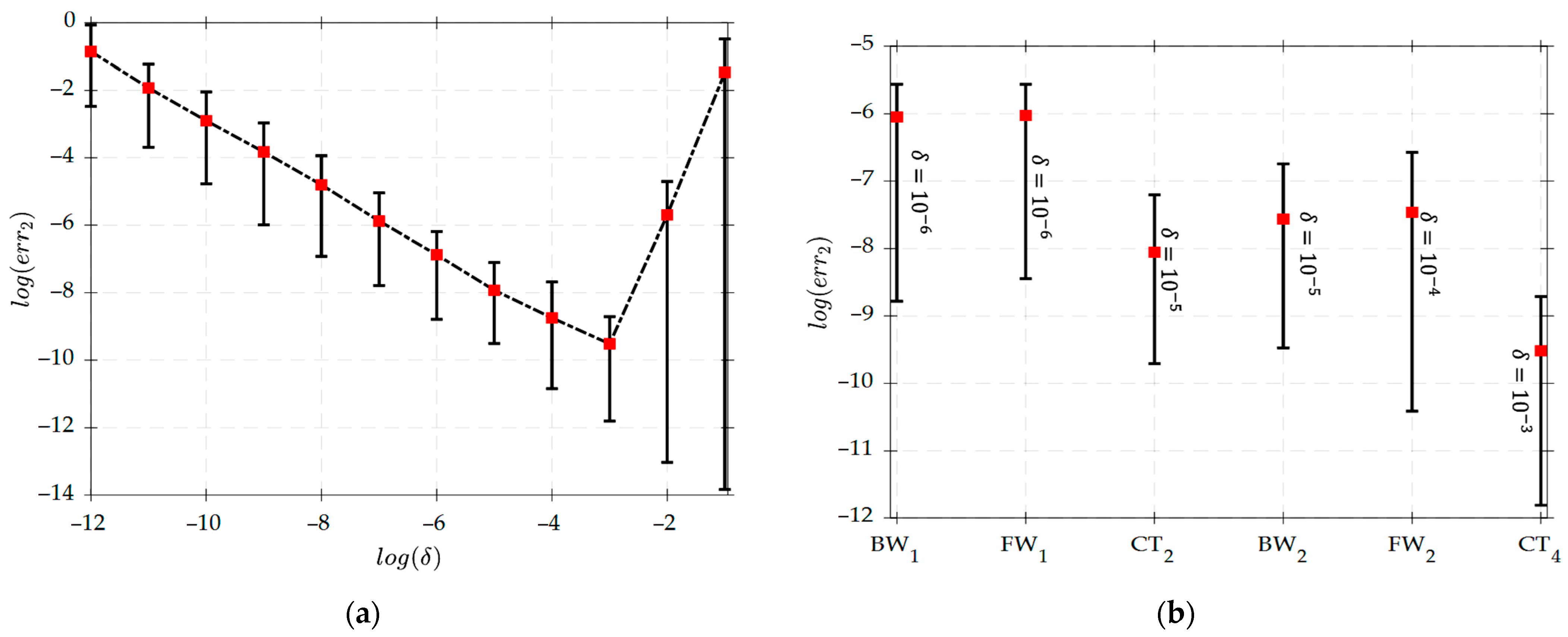
Values of e r r 2 from Equation (125) appear in Table 3, Table 4 and Table 5 for the various 2nd order orientation tensor models, identified in the left most column, and 4th order closure approximations, as identified in the table headers. The results show that with a perturbation size of δ = 10 6 , the e r r 2 magnitude values are below 10 6 which ensures the accuracy of our exact Jacobian derivations and numerical implementations over the various 2nd order orientation tensor models and 4th order closures approximations considered above. The e r r 2 magnitude values appear lower for the Hinch and Leal closure approximations (cf. Table 3) on the order of 10 9 10 8 as compared to the EBF and IBF closures (cf. Table 4), which is on the order of 10 8 . Alternatively, the e r r 2 magnitude values for the IBOF and EBOF closures (cf. Table 5) are relatively higher on the order of about 10 7 . In Figure 2a, the e r r 2 is shown to decrease monotonically with increasing perturbation size, showing the optimum result for δ = 10 3 , below which e r r 2 increases monotonically. Additionally, Figure 2b shows that the e r r 2 depends on the finite difference type and decreases with increasing order of approximation. Values of e r r 2 are relatively higher with lower order finite difference approximations (i.e., the 1st order backward and forward difference B W 1   a n d   F W 1 , respectively) and lower with higher order approximations (i.e., the 4th order central difference C T 4 ).

3.2. Comparison of the NR Method and the Dormand-Prince Runge–Kutta (RK45) Method

In this section, computed results of the steady state orientation states obtained for various orientation evolution models and closure approximations using our Newton Raphson algorithm are compared to those obtained using the RK45 method. The RK45 method is implemented to provide transient solutions to the initial-value orientation ODE (cf. Equation (7)). A sufficiently small time step is selected for the RK45 simulations to minimize truncation errors [44] and the computations are performed until steady state is achieved, defined where the Euclidean norm of the orientation tensor material derivative is less than 10 6 , i.e., at e r r R K 45 t = R _ i j R K 45 t 2 ,    R _ i j R K 45 t = a i j R K 45 / t .
Three sample cases are included here; the first set of models is based on the study by Falvoro et al. [23], and two other sets are based on the study by Tseng et al. [10]. These cases are used to assess the performance of the NR method relative to the RK4 method for steady state predictions based on various 2nd order orientation tensor models. The first case includes various anisotropic rotary diffusion (ARD) tensor models presented in [23] that account for fiber-fiber and fiber-matrix interactions. The second case considers slow orientation kinetics (SOK) tensor-based models such as the SRF, RSC, and RPR that correct the over-prediction inaccuracies of the transient fiber orientation response computed with the AT model. These models account for the effect of both deformation and diffusion of the fibers and matrix on the transient fibers response [10]. The third case is based on coupled tensor models involving a combination of an ARD model and an SOK model that has been shown to yield improved orientation tensor accuracy including the iARD-RPR and pARD-RPR which have been incorporated into Moldex3D (CoreTech System Co. of Taiwan) [19] and iARD-RSC models incorporated into AutoDesk MoldFlow® (Autodesk Inc., San Francisco, CA, USA). The models in the latter case study are typically used in injection molding simulations specifically for long-fiber concentrated suspensions [10,22]. The EBOF closure approximation of Verweyst [32] is employed for all analyses.
Case 1: The first study considers various anisotropic rotary diffusion (ARD) orientation tensor models with model parameters appearing in Table 2. The initial orientation state for the RK45 simulations is
a _ _ 0 = 0.30 0.00 0.00 0.00 0.60 0.10 0.00 0.10 0.10
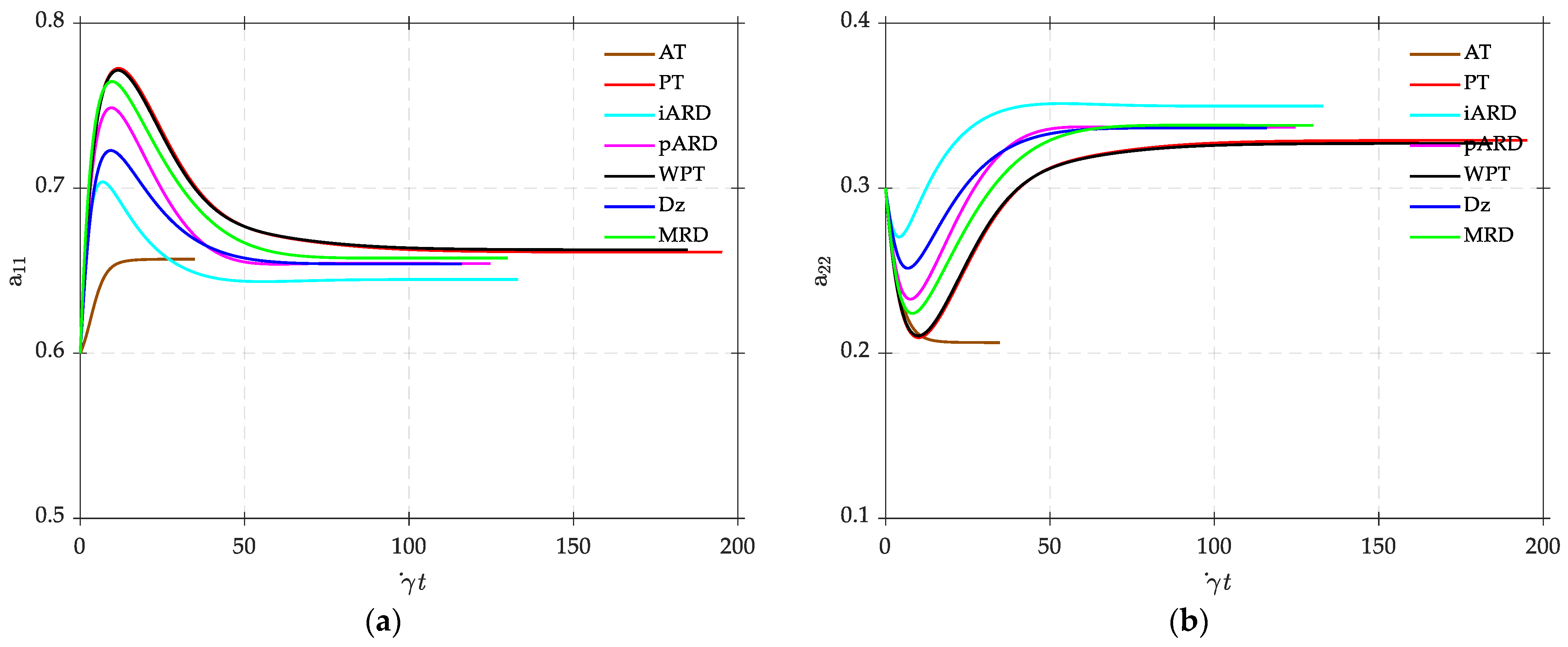
which is the same as that used as the initial guess in the NR method calculations. The initial guess value is selected such that the target steady state orientation is physical with non-negative eigenvalues in all cases. This is required for some tensor models that can exhibit numerical convergence instability such as the PT model [10,23]. One purpose of this first case study is to show that the NR method adequately predicts the steady state orientation irrespective of the choice and complexity of the rotary diffusion model or transient simulation behavior. The RK45 calculated transient responses for select components of a i j , and the results appear in Figure 3.
The computed responses in Figure 3a,b show varying amplitudes of initial overshoot of a 11 and initial trough of a 22 depending on the orientation model that do not affect the final steady state orientation. Table 6 includes values of e r r 1 (cf. Equation (121)) which show that the NR-based steady state orientation predictions agree well with RK4 values indicated by e r r 1 < 0.005 % for both diagonal and off-diagonal tensor components. Although the NR method does not provide information about the transient orientation history such as the initial overshoot and/or the initial trough, steady state orientations appear to be independent of the transient behavior of the orientation tensor model.
The NR convergence history for the various diffusion tensor models appears in Figure 4, which indicates a relatively higher rate of convergence with a quadratic nature for the fundamental AT isotropic rotary diffusion (IRD) model, requiring only 5 iterations for convergence compared to the PT, WPT, Dz, ARD models, which all required 7 iterations to converge. The improved and principal ARD models (iARD and pARD) show the slowest convergence rate, requiring 8 iterations to converge. All models, however, exhibit stable convergence with a monotonically decreasing NR residual norm. With the RK45 method, the orientation tensor reached steady state faster for the AT model, at a time fraction of γ ˙ t = 35 s compared to the iARD, pARD, Dz, and MRD models, which required an average of about γ ˙ t = 126 s to converge. The PT and WPT models were the slowest, requiring at least γ ˙ t = 185 s for the orientation to approach steady state. Unlike the AT, PT, and WPT models, the iARD, pARD, Dz, and MRD model transient responses had undulations, which may be an effect of the numerical solver due to the stiffness of the ODE.
In terms of computational efficiency, computation time was obtained for all NR and RK5 simulations using a x64-based, Intel(R) Core(TM) i5-8365U CPU with a 1.90 GHz processing speed and a 16.0 GB RAM, operating on Windows 11 Pro. The average computation time for each technique appears in Table 7. Overall, the NR technique is seen to be, on average, 7.4 x faster than the RK45 method for the error tolerance given in Table 6.
Case 2: Unlike the first case study, Case 2 investigates the behavior of the NR method for SOK tensor models that involves corrections to slow down the transient fiber orientation kinematic response as compared to the AT model, which includes the SRF, RSC and RPR models. Although the various model corrections have no effect on the final steady state solution, the effect of the SOK model complexity on NR convergence is shown. The model parameters used for this case study are taken from Tseng et al. [10] and appear in Table 8.
The starting orientation for the RK45 analysis and the initial guess a _ _ 0 used for the Newton Raphson method is the same as that used in case study 1 (cf. Equation (124)). Two flow fields L1 and L2 are considered:
  • L1: Simple shear flow in the 1–2 plane, L 12 = γ ˙ .
  • L2: Balanced shear/planar-elongation flow, simple shear in 1-2 plane superimposed on planar elongation in 1–2 plane. L 11 = ε ˙ , L 22 = ε ˙ , L 12 = γ ˙ given that γ ˙ / ε ˙ = 10 .
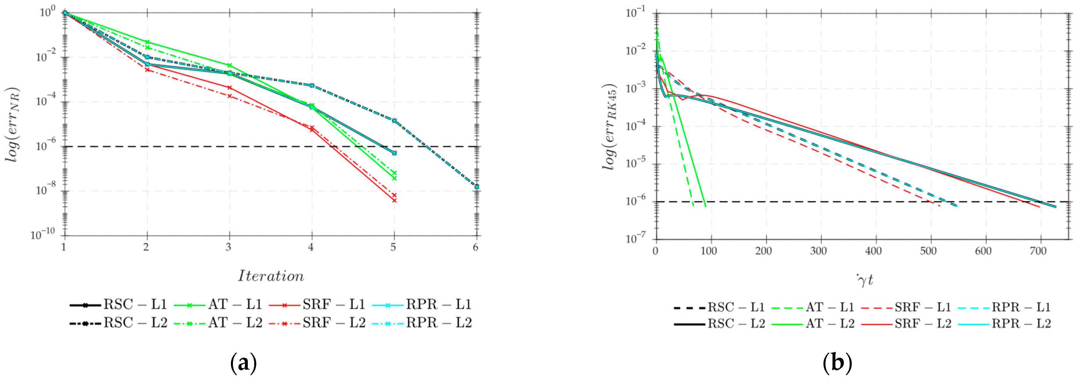
The time evolution of the components of the 2nd order orientation tensor based on the RK45 method are shown in Figure 5 below.
The percentage error between NR and RK45 steady state values are presented in Table 9. The results show a high level of accuracy in prediction based on the NR method, with a maximum error tolerance of only e r r 1 < 0.04 % among all tensor components for all models. The AT and SRF models exhibited relatively faster convergence rate requiring only 5 iterations to converge for both flow types (cf. Figure 6) compared to the RSC and RPR models which required an extra iteration to converge. The orientation tensor reached steady state faster with the AT tensor model compared to other tensor models in Figure 5 because the RK45 residual approached the set tolerance value of 10 6 faster than other tensor models (cf. Figure 6b). The RSC and RPR models both require complex eigenvalue and eigenvector spectral decompositions which may influence the convergence rate. Moreover, the derivatives of the eigenvectors as shown in Appendix A may impact the convergence rate of these models. The convergence rate was seen to be independent of both flow types considered.
Figure 7a,b present the NR residual norm for the AT and RSC models and for different initial orientation states obtained by varying a 22 0 (i.e.,   0 . a 22 0 0.7 ) while retaining the initial states of other a i j 0 components. As a 22 0 increases, the initial orientation states approach the final steady state orientation; thus, less iterations are required for the solutions to converge. The AT converged as expected for all a 22 0 values considered (cf. Figure 7a); however, the RSC model was very sensitive to the a 22 0 values (cf. Figure 7b). Only the initial orientation states with a 22 0 = 0.49 ,   0.56 ,   0.63 ,   0.70 converged to physical solutions (as shown in Figure 7b), while the other a 22 0 values yielded non-physical solutions.
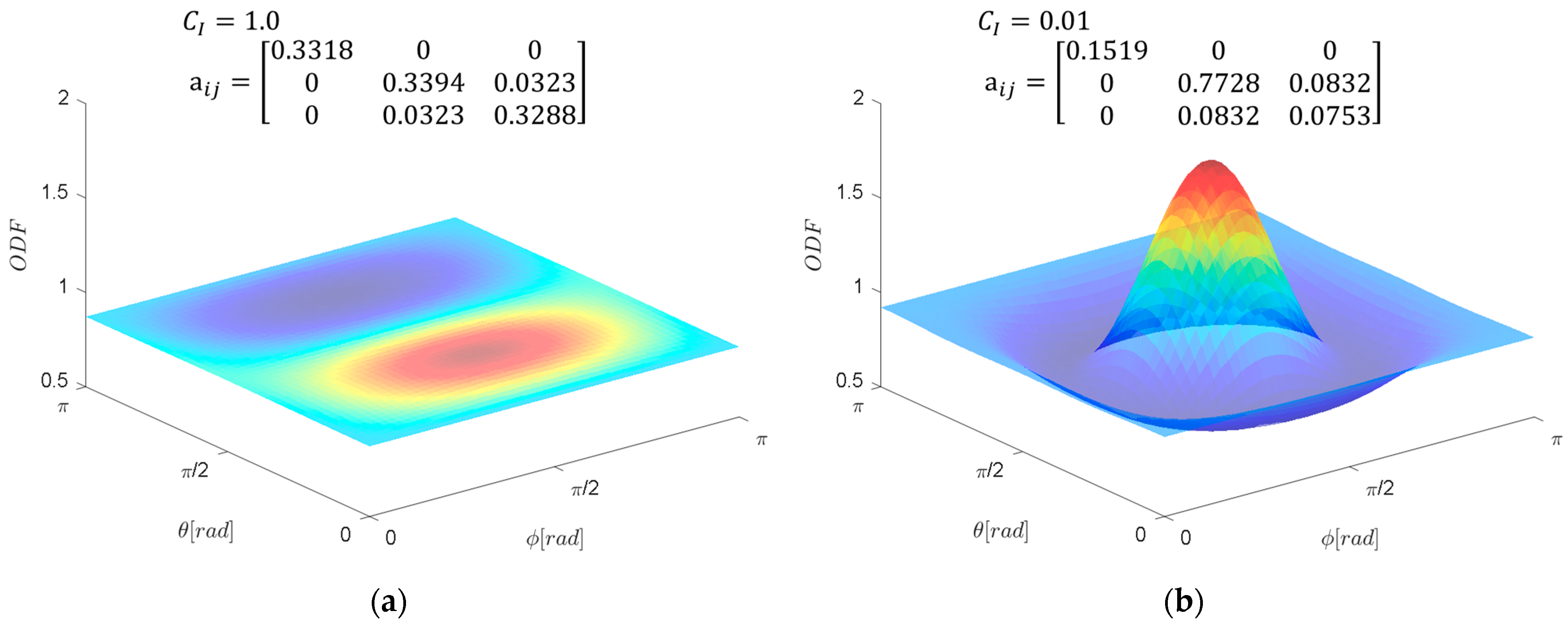
For the purpose of visualization, we present a typical 3D orientation distribution function (ODF) (cf. Figure 8) recovered from the deviatoric forms of the average steady state 2nd and 4th order fiber orientation tensors obtained from the NR solutions for two fiber interaction coefficients (CI = 0.01 and CI = 1.0) using the AT model and based on the method of Onat and Leckie [7].
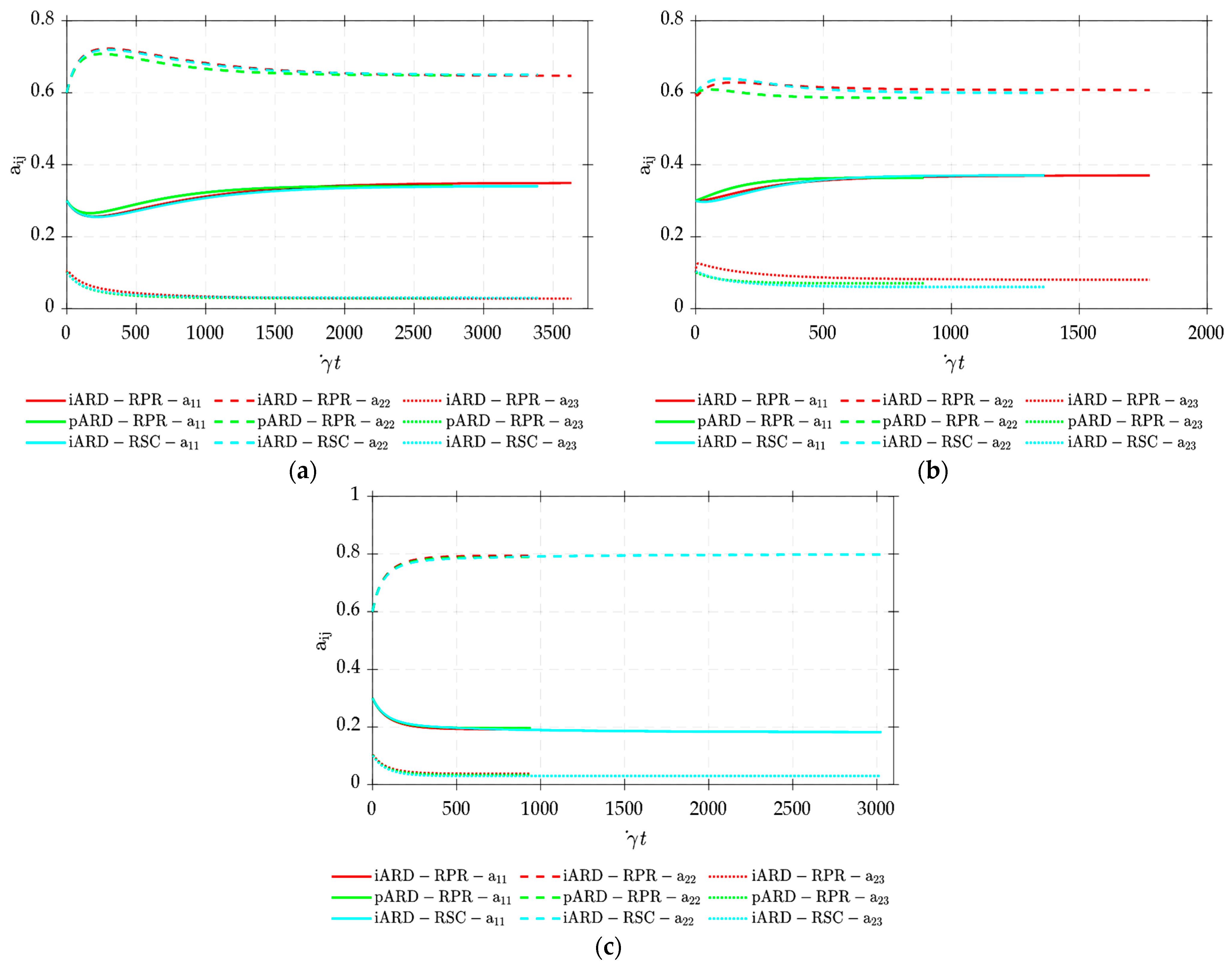
Case 3: The third case study investigates the performance of the NR method to coupled iARD-RPR and pARD-RPR orientation tensor models and includes model parameters to simulate three different polymer composites materials in simple shear flow with γ ˙ = 1 s 1 . The model parameters used for the three coupled models and three polymer composites (i.e., M1: 40 wt. % glass-fiber/PP, M2: 31 wt. % carbon-fiber/PP and M3: 40 wt. % glass-fiber/nylon) considered in this case study appear in Table 10 and Table 11. We assume the same RK45 initial orientation state and NR initial guess as in case study 1 (cf. Equation (124)). The simulated RK45 results for the coupled orientation models and polymer composites considered here appear in Figure 9a–c. The percentage error between the NR and RK45 steady state values are given in Table 12. The results show negligible discrepancy in the calculated steady state solutions, generally yielding an error e r r 1 below 0.3 % for all tensor components. Figure 10a, however, shows that the NR convergence rate is dependent on the model and composite material composition. The M2 (31 wt. % carbon-fiber/PP) with lower fiber content had a faster convergence rate for all three coupled tensor models compared to the M1 and M3 composites with higher fiber content which had a slower convergence rate. The coupled models showed slight instability through the initial NR iterations, especially for the iARD-RPR model with M1. The RK45 convergence profiles (cf. Figure 10b) is seen to have similar behavior as the NR convergence profiles in terms of the order of convergence for the various models and material types.

3.3. Performance of NR Method Using Various Closure Approximations

The performance of the NR method in computing steady state orientation tensor component values for various closure approximations of the 4th order orientation tensor in terms of accuracy and stability is assessed in this section. For this assessment, we consider the AT model with C I = 0.01 . The same initial orientation state for the RK45 method and the NR method’s initial guess used in case 1 of the preceding section (cf. Equation (124)) is also employed, and simple shear flow with γ ˙ = 1 s 1 is used for all analyses. The first set of results are presented for Hinch and Leal (HL) closures in Section 2.5.4 and for fitted closures in Section 2.5.5.
Figure 11a–d show the transient response of the a 11   a n d   a 12 from RK45 analysis through steady state. These results show that the choice of closure approximation affects the time taken to reach a steady state orientation. The model with the QDR and HYB2 closures reached steady-state faster than other models, while models with the LIN, ISO and SF2 closures required more time to reach steady-state. As shown in Table 13, the NR method results tend to agree well with RK45 reference values, having a maximum e r r 1 = 0.004 % . Likewise, NR simulations using the fitted closure approximations performed well with a good accuracy in predicted results (cf. Table 13). Figure 12a shows that the LIN and ISO closures had the fastest convergence rate with a quadratic nature, requiring only 3 iterations to converge followed by the HL1, HL2, QDR and HYB1 closures, which required 6 iterations to converge. The invariant-based HYB2 closure required an extra iteration to converge, while the SF2 closure had the slowest convergence rate, requiring up to 10 iterations to converge. Surprisingly, all the fitted closure approximations had similar convergence behavior, with only 5 iterations needed to converge except the IBOF closure, which required an extra iteration to converge (cf. Figure 12b). Conversely, RK45 convergence using the Hinch and Leal closures (cf. Figure 12c) has a rather distinct behavior, with the LIN, ISO and SF2 closures having the slowest convergence rate and the HYB2 and QDR closures having the fastest convergence rate. Similarly to the NR results that were obtained using fitted closures, the RK45 simulations converged over a narrower range (cf. Figure 12d) as compared to the Hinch and Leal closures.

3.4. Homogenous Flow Considerations

In this section we employ six homogenous flows to ensure the stability of our NR method beyond simple shear flow. The following flow conditions taken from [48] were considered:
  • SS: Simple shear flow in the 2–3 plane, i.e., L 23 = γ ˙ .
  • SUA: Two stretching/shearing flows, including simple shear in 2–3 plane superimposed with uniaxial elongation in 3-direction, i.e., L 11 = ε ˙ ,    L 22 = ε ˙ ,     L 33 =   2 ε ˙ ,   L 23 =   γ ˙ . Two cases are considered, including balanced shear/stretch with γ ˙ / ε ˙ = 10 and dominant stretch with γ ˙ / ε ˙ = 1 .
  • UA: Uniaxial elongation flow in the 3—direction, i.e., L 11 = L 22 = ε ˙ ,    L 33 =   2 ε ˙ .
  • BA: Biaxial elongation (BA) flow in the 2–3 plane, i.e.,   L 11 =   2 ε ˙ ,    L 22 = L 33 = ε ˙ .   
  • PST: Two shear/planar-elongation flows, including simple shear in 2–3 plane superimposed on planar elongation in 1–3 plane, L 11 =   ε ˙ ,    L 33 =   ε ˙ ,    L 23 =   γ ˙ . Two cases are considered, including balanced shear-planar elongation with γ ˙ / ε ˙ = 10 and dominant planar elongation with γ ˙ / ε ˙ = 1 .
  • SBA: Balanced shear/bi-axial elongation flow, including simple shear in 2–3 plane superimposed on biaxial elongation, i.e., L 11 = 2 ε ˙ ,   L 22 = L 33 =   ε ˙ ,   L 23 =   γ ˙ . Two cases are considered for the shear to extension rate, γ ˙ / ε ˙ = 1 and γ ˙ / ε ˙ = 10 .
The natural orthotropic closures, i.e., exact midpoint fit, NAT1, was employed for this study. The initial orientation state for the RK4 simulations and the initial guess a _ _ 0 for the NR iterations is
a _ _ 0 = 0.40 0.00 0.00 0.00 0.00 0.10 0.00 0.10 0.45
The NR method provided exceptional prediction accuracy of the orientation tensor components for all flow conditions considered where the percentage error for all orientation tensor components was zero to four decimals (i.e., e r r 1 = 0.0000 % ). Figure 13a,b show transient results for a 33   a n d   a 23 from RK45 simulations, respectively. The NR iteration history for the same (cf. Figure 13c) shows that a higher shear-to-extension rate ratio improves the NR rate of convergence. The SS, PST2, SUA2, and SBA2 flows converged faster than other flow types. Conversely, the flow types with the highest extension-to-shear rate ratio (UA and BA) had a slower rate of convergence. Alternatively, the RK45 solution (cf. Figure 13d) showed that the higher extension-to-shear rate ratio enhanced the convergence rate, contrary to what was observed for the NR convergence history. The behavior of both NR and RK45 numerical techniques under the various flow and model considerations can provide useful insights when selecting a suitable numerical technique for solving a particular problem.

4. Conclusions

A Newton-Raphson (NR) method was derived and implemented for computing steady state 2nd order fiber orientation tensors in homogeneous flows using exact 4th order Jacobians. Analytical expressions are provided for the Jacobians which are derived from partial derivatives of 2nd order fiber orientation tensor material derivatives taken with respect to the 2nd order fiber orientation tensor itself. Various macroscopic fiber orientation moment-tensor models and closure approximations of the 4th order fiber orientation tensor are included in the derivations, and the performance of the NR method in various homogenous flows have been studied.
In summary, our results show that
  • The computed exact Jacobians aligned closely with finite difference approximations for all fiber orientation tensor models and 4th order fiber orientation tensor closure approximations considered, and the degree of alignment depended on the perturbation size, finite difference type and finite difference order of approximation.
  • The steady state orientation predictions from the NR solutions matched closely with the results predicted by the RK45 method for all fiber orientation tensor models, 4th order fiber orientation tensor closure approximations and homogenous flow types considered in this paper. The NR method was observed to be comparatively faster than the RK45 method for computing steady state values of the second order orientation tensor in all cases.
  • The NR convergence and stability behavior depended on the type and complexity of the fiber orientation tensor model, the initial guess of the orientation tensor and the material properties of the underlying composite material. A good initial guess resulted in faster and more stable convergence to physical steady state solutions.
  • The NR convergence behavior also depended on the flow type and extension-to-shear rate ratio. Higher shear rate dominance and flow symmetry increased the NR convergence rate and vice versa.
Overall, the NR method for determining the steady state orientation tensor performed well in terms of accuracy and computational efficiency for all fiber orientation tensor models, 4th order fiber orientation tensor closure approximations and homogenous flows considered in this article.

Author Contributions

Conceptualization, A.E.A. and D.E.S.; methodology, A.E.A. and D.E.S.; software, D.E.S.; validation, A.E.A. and D.E.S.; formal analysis, A.E.A.; investigation, A.E.A.; resources, D.E.S.; data curation, A.E.A.; writing—original draft preparation, A.E.A.; writing—review and editing, D.E.S.; visualization, A.E.A.; supervision, D.E.S.; project administration, D.E.S.; funding acquisition, D.E.S. All authors have read and agreed to the published version of the manuscript.

Funding

This research was funded by the National Science Foundation (NSF), grant number 2055628.

Data Availability Statement

The data presented in this study are available upon request from the corresponding author due to privacy restrictions.

Conflicts of Interest

The authors declare no conflicts of interest.

Appendix A

Appendix A.1. Eigenvalues and Eigenvector Derivatives

The eigenvalue for a matrix a _ _ is often given in terms of the eigenvalues λ k and corresponding eigenvectors Φ _ k as [49]
a _ _ λ k I _ _ Φ _ k = F _ k
For the homogeneous system F _ k = 0 , requiring Φ _ k 0 to yield non-trivial solutions, Equation (A1) becomes a _ _ λ k I _ _ = 0 , where the vertical bars indicate the matrix determinant. The resulting system matrix a m n λ k δ m n is known to be rank deficient by an order of 1, requiring that we impose a normalization condition on the eigenvectors Φ _ k which can be defined through a scalar function G k Φ _ k = 0 . The eigenvectors are thus obtained by replacing the nth row of the residual column vector Σ i k = a i j λ k δ i j Φ j k F _ i k with G k Φ _ k = 0 and solving for Φ _ k from the equation Σ _ k Φ _ k = 0 through any iterative algorithm or explicit solver. Here, we employ Newton-Raphson’s method to obtain Φ _ k such that
Φ _ k + = Φ _ k J _ _ k 1 Σ k
Σ i k = S i j k Φ j k F _ i k i n G k Φ _ k i = n
J i j k = Σ i k Φ j k = S i j k i n G k Φ j k i = n
where
S i j k = a i j λ k δ i j
The derivative of the eigenvalues with respect to components a i j can thus be obtained by differentiating Equation (A3), assuming symmetry of system matrix, i.e., S i j k = S j i k , such that
Φ i k S i j k a r s Φ j k + F _ i k Φ i k a r s Φ i k F i k a r s = 0
Φ i k S i j k = S j i k Φ j k = S i j k Φ j k = F _ i k
where
S i j k a r s = δ i r δ j s λ k a r s δ i j
Assuming F _ i k = 0 , we obtain
λ k a r s = 1 Φ m k Φ m k Φ r k Φ s k
Consequently, we can determine the corresponding derivatives Φ i k / a r s given λ k / a r s from
S i j k Φ i k a r s = S j i k a r s Φ i k
Recalling that the system matrix a _ _ λ k I _ _ is inherently singular, we can substitute an nth row of the above equation by adopting a normalization technique [49]:
G k Φ j k Φ j k a r s = G k a r s
The modified differential equation can be recast as given in Equation (A12) below, allowing the inversion of the modified system matrix to solve
J i j k Φ i k a r s = Q i k a r s
where
Q i k a r s = S i j k a r s Φ j k i n G k a r s i = n
Smith et al. [49] presents three common normalization techniques:
  • ‘Mass’ Normalization
G k Φ _ k = Φ j k Φ j k 1 ,    G k Φ j k = 2 Φ j k ,    G k a r s = 0
2.
Preassigning an mth Component of Φ _ k
G k Φ _ k = δ m j Φ j k α ,    G k Φ j k = δ m j ,    G k a r s = 0
3.
Predefining the Euclidean norm of Φ _ k
G k Φ _ k = Φ j k Φ j k β ,    G k Φ j k = Φ j k ,    G k a r s = 0

Appendix B

Appendix B.1. Optimal Fitted Closure Approximation Constants/Coefficients

Appendix B.1.1. Eigenvalue-Based Optimal Fitting Closure (EBOF) Approximation

In the main body of the paper, we presented the generalized formulations for the eigenvalue-based orthotropic binomial fitted closure approximation which is written in terms of a constant coefficient matrix C i j n and an nth order permuted bivariate polynomial vector j n with n + 1 n + 2 / 2 number of parameters (cf. Equations (101)–(103)). Depending on the polynomial order n the various constants and coefficient matrix C _ _ ( n ) for the closures considered in this paper taken from Kuzmin [38] are presented below.
  • Linear Orthotropic Fitted Closure n = 1  
For the orthotropic linear (ORT) closure, the constant coefficient matrix C _ _ ( 1 ) is given as
C _ _ 1 = 1 7 3 / 5 6 0 3 / 5 0 6 27 / 5 6 6
and for the orthotropic fitted closure by Cintra and Tucker (cf. [39]), the constant coefficient matrix C _ _ ( 1 ) is given as
C _ _ 1 = 0.15 1.15 0.10 0.15 0.15 0.90 0.60 0.60 0.60
2.
Quadratic Orthotropic Fitted Closures n = 2
The simple general orthotropic quadratic closure has a constant coefficient matrix C _ _ ( 2 ) given as
C _ _ 2 = 0 0 0 1 0 0 0 0 0 0 0 1 1 2 2 1 2 1
The orthotropic natural closure—exact midpoint fit (NAT1) [38] has a constant coefficient matrix C _ _ ( 2 ) given as
C _ _ 2 = 0.0708 0.3236 0.3776 0.6056 0.4124 0.3068 0.0708 0.2792 0.2252 0.2084 0.4124 0.7040 1.1880 2.0136 2.1264 0.8256 1.7640 0.9384
The ORF independent coefficients are derived from a 2nd order polynomial fit of the principal axis data obtained from DFC via a minimization technique. For the orthotropic fitted closure by Cintra and Tucker (ORF) (cf. [39]), the constant coefficient matrix C _ _ ( 2 ) is given as
C _ _ 2 = 0.060964 0.371243 0.369160 0.555301 0.371218 0.318266 0.124711 0.389402 0.086169 0.258844 0.544992 0.796080 1.228982 2.054116 2.260574 0.821548 1.819756 1.053907
Chung and Kwon [56] improved the ORF and developed the 2nd order ORW closure for wide interaction coefficients that proved to be stable for all flow conditions considered. The improved orthotropic fitted closure (ORW2) by Chung and Kwon (cf. [56]) has a constant coefficient matrix C _ _ ( 2 ) given as
C _ _ 2 = 0.070055     0.339376 0.396796 0.590331 0.411944 0.333693 0.115177 0.368267     0.094820 0.252880   0.535224   0.800181 1.249811 2.148297 2.290157 0.898521 1.934914 1.044147
Kuzmin [38] presents details on derivations of some orthotropic fitted closures via a numerical bottom-up approach.
3.
Cubic Orthotropic Fitted Closures n = 3
Recently, higher order polynomial fitted closures were developed for improved accuracy. Although, the orthotropic natural closure—extended quadratic fit (NAT2) has a cubic order, it is essentially quadratic.
  • Non-rational Fitted Closure
The constant coefficient matrix C _ _ 3 for this closure approximation is given as
C _ _ 3 = 0     0.5 0 0.5 0.6 0 0 0.6 0.6 0 0 0     0.5 0 0.6 0.5 0 0.6 0.6 0 1 1.5 1.5 0.5     0.4 0.5 0 0.6 0.6 0
Chung and Kwon [56] also extended the 2nd order ORW to develop a 3rd order polynomial ORW3 closure using new flow data from ODFC calculation. For the improved 3rd order orthotropic fitted closure ORW3 by Chung and Kwon [56], the constant coefficient matrix is given as
C _ _ 3 T = 0.1480648093 0.2106349673 0.4868019601 0.8084618453 0.9092350296 0.5776328438 0.7765597096 1.1104441966 0.4605743789 0.3722003446 1.2840654776 2.2462007509 1.7366749542 2.5375632310 4.8900459209 1.3431772379 0.1260059291 1.9088154281 0.0324756095 0.5856304774 1.1817992322 0.8895946393 1.9988098293 4.0544348937 1.7367571741 1.4863151577 3.8542602127 0.6631716575 0.0756740034 0.9512305286
Eigenvalue-based optimal fitting (EBOF) closures were developed, which are extensions to the ORF but with higher order polynomial fits for improved accuracy. These include the rational elliptical (RE) closure by Wetzel [54] and the 4th order polynomial fitted closure by Verweyst [53] (VST).
  • Rational Fitted Closure
The rational elliptical (RE) closure developed by Wetzel [41] is a higher order extension to the ORF using Carlson elliptical integrals. The rational ellipsoid fitted closure has two permutation vectors, with the denominator being one order less than the numerator, i.e., m = n 1 , which is of cubic order, n = 3 . The corresponding constant coefficient matrix for the Wetzel numerator n = 3 is [54]
C _ _ 3 T = 0.1433751825 0.1433751825 0.9685744898 0.6566650339 0.5209453949 2.5526857671 0.5106016916 0.6463213306 2.5756669706 3.5295952199 0.6031924921 2.2044050704 4.4349137241 2.3303190917 4.4520903005 0.1229618909 5.1539592511 2.2485545147 2.9144388828 0.2256222796 0.6202937932 5.5556896198 1.6481269200 1.8811803355 2.8284365891 5.4494528976 1.9023485762 0.2292109036 3.7461520908 0.6414620339
And for the denominator m = n 1 = 2 ,
C _ _ 2 T = 1.0000000000 1.0000000000 1.0000000000 0.7257989503 0.6916858207 1.2134964928 3.0941511876 3.1282643172 1.2128608265 1.6239324646 1.5898193351 0.2393747647 4.7303686308 4.7303686308 0.6004510415 3.1742364608 3.2083495904 0.2162486576
Mullens M. [40] developed several high order polynomial fitted closures for short fiber composites and introduced the time derivative fitted closures. For the LAR32 closure by Mullens M. [40], the corresponding constant coefficient matrix for the numerator n = 3 is
C _ _ 3 T = 0.087602233 0.156805152 1.072423739 0.028205550 0.577818864 2.803554028 0.426784335 0.514280920 2.661576129 1.274677110 0.684250887 2.389379765 0.876469059 2.132305029 4.566728489 0.602031647 3.454835266 2.097523143 1.066583115 0.263237143 0.658248930 1.918931146 1.614122610 1.904704744 0.934291306 4.005261132 1.754978355 0.262854903 2.228133231 0.508282668
And for the denominator m = n 1 = 2 ,
C _ _ 2 T = 1.000000000 1.000000000 1.000000000 0.244001948 0.365652907 1.068512526 0.574150861 1.385725477 0.771356469 0.432097367 1.359687152 0.067386858 0.895226091 2.866357848 0.206908269 0.462709527 1.518996192 0.248999874
4.
Quartic Orthotropic Fitted Closures n = 4
The constant coefficient matrix C _ _ based on a regression analysis by Verweyst [53] developed from Carlson elliptic integrals is
C _ _ 4 T = 0.6363 0.6363 2.7405 1.8727 3.3153 9.1220 4.4797 3.0371 12.2571 11.9590 11.8273 34.3199 3.8446 6.8815 13.8295 11.3421 8.4368 25.8685 10.9583 15.9121 37.7029 20.7278 15.1516 50.2756 2.1162 6.4873 10.8802 12.3876 8.6389 26.9637 9.8160 9.3252 27.3347 3.4790 7.7468 15.2651 11.7493 7.4815 26.1135 0.5080 2.2848 3.4321 4.8837 3.5977 10.6117
The constant coefficient matrix C _ _ based on a regression analysis for the FFLAR4 closure by Mullens [40] is
C _ _ 4 T = 0.678225884 0.748226727 3.167356369 3.834359034 4.249612053 13.288266400 2.664862865 2.987266447 11.680179330 9.746185193 8.641488072 23.788431340 14.209962670 14.938209410 43.700607680 2.700369681 5.974489008 17.383121430 8.013024236 7.521216405 19.959054610 22.447252700 21.757217160 58.354308000 13.078649640 15.798676320 49.513705640 0.125467689 3.616551654 11.755525930 2.417857515 2.376441613 6.291273472 10.563248410 10.222185780 25.844317920 12.689484570 12.640352670 35.425354130 2.487386515 4.788201652 18.226443930 0.328195677 1.056519961 2.925785795
The constant coefficient matrix C _ _ based on a regression analysis for the LAR4 closure by Mullens [40] is
C _ _ 4 T = 0.813175172 1.768619587 4.525066937 3.065410883 9.826017151 19.259137620 4.659333003 6.484058476 17.650178090 6.329870878 19.986994700 33.901239610 14.747639770 28.905936750 61.543979540 9.739797775 10.759963010 28.467355970 4.216519964 17.715409270 27.768082700 15.922240910 40.492387100 76.738638810 20.818571900 27.442217500 68.977583290 8.993993112 7.230748101 22.399036130 1.138888034 5.785725498 8.600822308 5.834142985 18.709047480 32.480679940 11.470974520 19.729631240 43.875135630 9.874209286 8.882877701 26.928320210 3.100457733 2.224834058 7.101978254

Appendix B.1.2. Invariant-Based Optimal Fitting Closure (IBOF) Approximation

The unknown independent coefficients of the binomial expansion for the six parameters in the IBOF closure representation based on regression fitting by Chung et al. [34] of actual flow data obtained from the distribution function closure considering different flow types like EBF closures are given in Table A1 below.
Table A1. The 5th order binomial fitting coefficients for the IBOF closure approximation.
k \ m 123
02.49409081657860 × 101−4.97217790110754 × 10−12.34146291570999 × 101
1−4.35101153160329 × 1022.34980797511405 × 101−4.12048043372534 × 10²
27.03443657916476 × 1031.53965820593506 × 1025.73259594331015 × 103
33.72389335663877 × 10³−3.91044251397838 × 1023.19553200392089 × 103
4−1.33931929894245 × 10⁵−2.13755248785646 × 10³−6.05006113515592 × 10⁴
58.23995187366106 × 1051.52772950743819 × 105−4.85212803064813 × 10⁴
6−1.59392396237307 × 1042.96004865275814 × 103−1.10656935176569 × 10⁴
78.80683515327916 × 10⁵−4.00138947092812 × 10³−4.77173740017567 × 10⁴
8−9.91630690741981 × 10⁶−1.85949305922308 × 1065.99066486689836 × 106
98.00970026849796 × 1062.47717810054366 × 106−4.60543580680696 × 10⁷
103.22219416256417 × 10⁴−1.04092072189767 × 1041.28967058686204 × 104
11−2.37010458689252 × 1061.01013983339062 × 1052.03042960322874 × 106
123.79010599355267 × 1077.32341494213578 × 106−5.56606156734835 × 10⁷
13−3.37010820273821 × 10⁷−1.47919027644202 × 1075.67424911007837 × 108
14−2.57258805870567 × 10⁸−6.35149929624336 × 10⁷−1.52752854956514 × 10⁹
15−2.32153488525298 × 1041.38088690964946 × 1044.66767581292985 × 103
162.14419090344474 × 10⁶−2.47435106210237 × 10⁵−4.99321746092534 × 10⁶
17−4.49275591851490 × 10⁷−9.02980378929272 × 1061.32124828143333 × 108
18−2.13133920223355 × 1077.24969796807399 × 106−1.62359994620983 × 10⁹
191.57076702372204 × 1094.87093452892595 × 1087.92526849882218 × 109
20−3.95769398304473 × 10⁹−1.60162178614234 × 10⁹−1.28050778279459 × 10¹⁰

References

  1. Jeffery, G.B. The motion of ellipsoidal particles immersed in a viscous fluid. Proc. R. Soc. Lond. Ser. Contain. Pap. Math. Phys. Character 1922, 102, 161–179. [Google Scholar] [CrossRef]
  2. Saffman, P.G. On the motion of small spheroidal particles in a viscous liquid. J. Fluid Mech. 1956, 1, 540–553. [Google Scholar] [CrossRef]
  3. Folgar, F.; Tucker, C.L. Orientation Behavior of Fibers in Concentrated Suspensions. J. Reinf. Plast. Compos. 1984, 3, 98–119. [Google Scholar] [CrossRef]
  4. Folgar Portillo, F. Fiber Orientation Distribution in Concentrated Suspensions: A Predictive Model. Ph.D. Dissertation/Thesis, University of Illinois at Urbana, Champaign, IL, USA, 1983. Available online: http://ezproxy.baylor.edu/login?url=https://www.proquest.com/dissertations-theses/fiber-orientation-distribution-concentrated/docview/303264729/se-2?accountid=7014 (accessed on 9 March 2023).
  5. Bay, R.S. Fiber Orientation in Injection-Molded Composites: A Comparison of Theory and Experiment. Ph.D. Dissertation/Thesis, University of Illinois at Urbana, Champaign, IL, USA, 1991. Available online: http://ezproxy.baylor.edu/login?url=https://www.proquest.com/dissertations-theses/fiber-orientation-injection-molded-composites/docview/303941981/se-2?accountid=7014 (accessed on 22 December 2021).
  6. Montgomery-Smith, S.; Jack, D.; Smith, D.E. The Fast Exact Closure for Jeffery’s equation with diffusion. J. Non-Newton. Fluid Mech. 2011, 166, 343–353. [Google Scholar] [CrossRef]
  7. Advani, S.G.; Tucker, C.L. The Use of Tensors to Describe and Predict Fiber Orientation in Short Fiber Composites. J. Rheol. 1987, 31, 751–784. [Google Scholar] [CrossRef]
  8. Huynh, H.M. Improved Fiber Orientation Predictions for Injection-Molded Composites. Master’s Thesis, University of Illinois at Urbana, Champaign, IL, USA, 2001. [Google Scholar]
  9. Wang, J.; O’Gara, J.F.; Tucker, C.L. An objective model for slow orientation kinetics in concentrated fiber suspensions: Theory and rheological evidence. J. Rheol. 2008, 52, 1179–1200. [Google Scholar] [CrossRef]
  10. Tseng, H.-C.; Chang, R.-Y.; Hsu, C.-H. Phenomenological improvements to predictive models of fiber orientation in concentrated suspensions. J. Rheol. 2013, 57, 1597–1631. [Google Scholar] [CrossRef]
  11. Tseng, H.-C.; Chang, R.-Y.; Hsu, C.-H. Method and Computer Readable Media for Determining Orientation of Fibers in a Fluid. U.S. Patent 8571828 B2, 29 August 2023. [Google Scholar]
  12. Phelps, J.H.; Tucker, C.L. An anisotropic rotary diffusion model for fiber orientation in short- and long-fiber thermoplastics. J. Non-Newton. Fluid Mech. 2009, 156, 165–176. [Google Scholar] [CrossRef]
  13. Ranganathan, S.; Advani, S.G. Fiber–fiber interactions in homogeneous flows of nondilute suspensions. J. Rheol. 1991, 35, 1499–1522. [Google Scholar] [CrossRef]
  14. Fan, X.; Phan-Thien, N.; Zheng, R. A direct simulation of fibre suspensions. J. Non-Newton. Fluid Mech. 1998, 74, 113–135. [Google Scholar] [CrossRef]
  15. Phan-Thien, N.; Fan, X.-J.; Tanner, R.I.; Zheng, R. Folgar–Tucker constant for a fibre suspension in a Newtonian fluid. J. Non-Newton. Fluid Mech. 2002, 103, 251–260. [Google Scholar] [CrossRef]
  16. Koch, D.L. A model for orientational diffusion in fiber suspensions. Phys. Fluids 1995, 7, 2086–2088. [Google Scholar] [CrossRef]
  17. Hand, G.L. A theory of anisotropic fluids. J. Fluid Mech. 1962, 13, 33–46. [Google Scholar] [CrossRef]
  18. Tseng, H.-C.; Chang, R.-Y.; Hsu, C.-H. An objective tensor to predict anisotropic fiber orientation in concentrated suspensions. J. Rheol. 2016, 60, 215–224. [Google Scholar] [CrossRef]
  19. Tseng, H.-C.; Chang, R.-Y.; Hsu, C.-H. The use of principal spatial tensor to predict anisotropic fiber orientation in concentrated fiber suspensions. J. Rheol. 2018, 62, 313–320. [Google Scholar] [CrossRef]
  20. Bakharev, A.Y.; Yu, H.; Ray, S.; Speight, R.; Wang, J. Using new anisotropic rotational diffusion model to improve prediction of short fibers in thermoplastic injection molding. In Proceedings of the 2018 Society of Plastics Engineers (SPE) International Polyolefins Conference, Lubbock, TX, USA, 25–28 February 2018. [Google Scholar]
  21. Latz, A.; Strautins, U.; Niedziela, D. Comparative numerical study of two concentrated fiber suspension models. J. Non-Newton. Fluid Mech. 2010, 165, 764–781. [Google Scholar] [CrossRef]
  22. Kugler, S.K.; Kech, A.; Cruz, C.; Osswald, T. Fiber Orientation Predictions—A Review of Existing Models. J. Compos. Sci. 2020, 4, 69. [Google Scholar] [CrossRef]
  23. Favaloro, A.J.; Tucker, C.L. Analysis of anisotropic rotary diffusion models for fiber orientation. Compos. Part Appl. Sci. Manuf. 2019, 126, 105605. [Google Scholar] [CrossRef]
  24. Agboola, B.O.; Jack, D.A.; Montgomery-Smith, S. Effectiveness of recent fiber-interaction diffusion models for orientation and the part stiffness predictions in injection molded short-fiber reinforced composites. Compos. Part A Appl. Sci. Manuf. 2012, 43, 1959–1970. [Google Scholar] [CrossRef]
  25. Park, J.M.; Park, S.J. Modeling and Simulation of Fiber Orientation in Injection Molding of Polymer Composites. Math. Probl. Eng. 2011, 2011, 105637. [Google Scholar] [CrossRef]
  26. Bay, R.S.; Tucker, C.L. Fiber orientation in simple injection moldings. Part I: Theory and numerical methods. Polym. Compos. 1992, 13, 317–331. [Google Scholar] [CrossRef]
  27. Bay, R.S.; Tucker, C.L. Fiber orientation in simple injection moldings. Part II: Experimental results. Polym. Compos. 1992, 13, 332–341. [Google Scholar] [CrossRef]
  28. Gupta, M.; Wang, K.K. Fiber orientation and mechanical properties of short-fiber-reinforced injection-molded composites: Simulated and experimental results. Polym. Compos. 1993, 14, 367–382. [Google Scholar] [CrossRef]
  29. Chung, S.T.; Kwon, T.H. Coupled analysis of injection molding filling and fiber orientation, including in-plane velocity gradient effect. Polym. Compos. 1996, 17, 859–872. [Google Scholar] [CrossRef]
  30. Vincent, M.; Devilers, E.; Agassant, J.-F. Fibre orientation calculation in injection moulding of reinforced thermoplastics. J. Non-Newton. Fluid Mech. 1997, 73, 317–326. [Google Scholar] [CrossRef]
  31. Vincent, M.; Giroud, T.; Clarke, A.; Eberhardt, C. Description and modeling of fiber orientation in injection molding of fiber reinforced thermoplastics. Polymer 2005, 46, 6719–6725. [Google Scholar] [CrossRef]
  32. VerWeyst, B.E.; Tucker, C.L.; Foss, P.H.; O’Gara, J.F. Fiber Orientation in 3-D Injection Molded Features: Prediction and Experiment. Int. Polym. Process. 1999, 14, 409–420. [Google Scholar] [CrossRef]
  33. Hinch, E.J.; Leal, L.G. Constitutive equations in suspension mechanics. Part 2. Approximate forms for a suspension of rigid particles affected by Brownian rotations. J. Fluid Mech. 1976, 76, 187–208. [Google Scholar] [CrossRef]
  34. Chung, D.H.; Kwon, T.H. Invariant-based optimal fitting closure approximation for the numerical prediction of flow-induced fiber orientation. J. Rheol. 2002, 46, 169–194. [Google Scholar] [CrossRef]
  35. Jack, D.A.; Smith, D.E. The effect of fibre orientation closure approximations on mechanical property predictions. Compos. Part A Appl. Sci. Manuf. 2007, 38, 975–982. [Google Scholar] [CrossRef]
  36. Quintana, M.C.; Frontini, P.M.; Arriaga, A.; Plank, B.; Major, Z. Fiber Orientation Distribution Predictions for an Injection Molded Venturi-Shaped Part Validated Against Experimental Micro-Computed Tomography Characterization. Front. Mater. 2020, 7, 169. [Google Scholar] [CrossRef]
  37. Jack, D.A. Advanced Analysis of Short-Fiber Polymer Composite Material Behavior. Ph.D. Thesis, University of Missouri, Columbia, MO, USA, 2006. [Google Scholar]
  38. Kuzmin, D. Planar Orthotropic Closures for Orientation Tensors in Fiber Suspension Flow Models. SIAM J. Appl. Math. 2018, 78, 3040–3059. [Google Scholar] [CrossRef]
  39. Cintra, J.S.; Tucker, C.L. Orthotropic closure approximations for flow-induced fiber orientation. J. Rheol. 1995, 39, 1095–1122. [Google Scholar] [CrossRef]
  40. Mullens, M. Developing New Fitted Closure Approximations for Short-Fiber Reinforced Polymer Composites. Master’s Thesis, University of Missouri, Columbia, MO, USA, 2010. Available online: https://core.ac.uk/download/pdf/62781195.pdf (accessed on 9 March 2023).
  41. Jack, D.A.; Schache, B.; Smith, D.E. Neural network-based closure for modeling short-fiber suspensions. Polym. Compos. 2010, 31, 1125–1141. [Google Scholar] [CrossRef]
  42. Qadir, N.U.; Jack, D.A. Modeling fibre orientation in short fibre suspensions using the neural network-based orthotropic closure. Compos. Part A Appl. Sci. Manuf. 2009, 40, 1524–1533. [Google Scholar] [CrossRef]
  43. Jack, D.A. Investigating the Use of Tensors in Numerical Predictions for Short-Fiber Reinforced Polymer Composites. Ph.D. Thesis, University of Missouri, Columbia, MO, USA, 2003. [Google Scholar]
  44. Chapra, S.C. Applied Numerical Methods with MATLAB for Engineers and Scientists, 3rd ed.; McGraw-Hill: New York, NY, USA, 2012. [Google Scholar]
  45. Tucker, C.L. Fundamentals of Fiber Orientation: Description, Measurement and Prediction; Hanser Publishers: Munich, Germany, 2022. [Google Scholar] [CrossRef]
  46. Eberle, A.P.R.; Ortman, K.; Baird, D.G. Structure and Rheology of Fiber Suspensions. In Applied Polymer Rheology, 1st ed.; Kontopoulou, M., Ed.; Wiley: Hoboken, NJ, USA, 2011; pp. 113–151. [Google Scholar] [CrossRef]
  47. Zhang, D. Flow-Induced Micro- and Nano-Fiber Suspensions in Short-Fiber Reinforced Composite Materials Processing. Ph.D. Thesis/Dissertation, University of Missouri, Columbia, MO, USA, 2013. Available online: http://ezproxy.baylor.edu/login?url=https://www.proquest.com/dissertations-theses/flow-induced-micro-nano-fiber-suspensions-short/docview/2202998717/se-2?accountid=7014 (accessed on 8 December 2020).
  48. Awenlimobor, A.; Smith, D.E. Effect of shear-thinning rheology on the dynamics and pressure distribution of a single rigid ellipsoidal particle in viscous fluid flow. Phys. Fluids 2024, 36, 123113. [Google Scholar] [CrossRef]
  49. Smith, D.E.; Siddhi, V. Generalized Approach for Incorporating Normalization Conditions in Design Sensitivity Analysis of Eigenvectors. AIAA J. 2006, 44, 2552–2561. [Google Scholar] [CrossRef]
  50. Wang, J. Moldflow Research & Development. Online. 2018. Available online: https://damassets.autodesk.net/content/dam/autodesk/www/campaigns/autodesk-moldflow-summit-recording/7_R&D-Update%20-%20Jin%20Wang.pdf (accessed on 9 March 2023).
  51. Doi, M. Molecular dynamics rheological properties of concentrated solutions of rodlike polymers in isotropic liquid crystalline phases. J. Polym. Sci. Polym. Phys. Ed. 1981, 19, 229–243. [Google Scholar] [CrossRef]
  52. Lipscomb, G.G.; Denn, M.M.; Hur, D.U.; Boger, D.V. The flow of fiber suspensions in complex geometries. J. Non-Newton. Fluid Mech. 1988, 26, 297–325. [Google Scholar] [CrossRef]
  53. VerWeyst, B.E. Numerical Predictions of Flow-Induced Fiber Orientation in Three-Dimensional Geometries. Ph.D. Dissertation/Thesis, University of Illinois at Urbana, Champaign, IL, USA, 1998. Available online: http://ezproxy.baylor.edu/login?url=https://www.proquest.com/dissertations-theses/numerical-predictions-flow-induced-fiber/docview/304440327/se-2?accountid=7014 (accessed on 18 February 2022).
  54. Wetzel, E.D.; Tucker, C.L. Area tensors for modeling microstructure during laminar liquid-liquid mixing. Int. J. Multiph. Flow 1999, 25, 35–61. [Google Scholar] [CrossRef]
  55. Verleye, V.; Couniot, A.; Dupret, F. Numerical prediction of fibre orientation in complex injection-moulded parts. WIT Trans. Eng. Sci. 1994, 4, 10. [Google Scholar] [CrossRef]
  56. Chung, D.H.; Kwon, T.H. Improved model of orthotropic closure approximation for flow induced fiber orientation. Polym. Compos. 2001, 22, 636–649. [Google Scholar] [CrossRef]
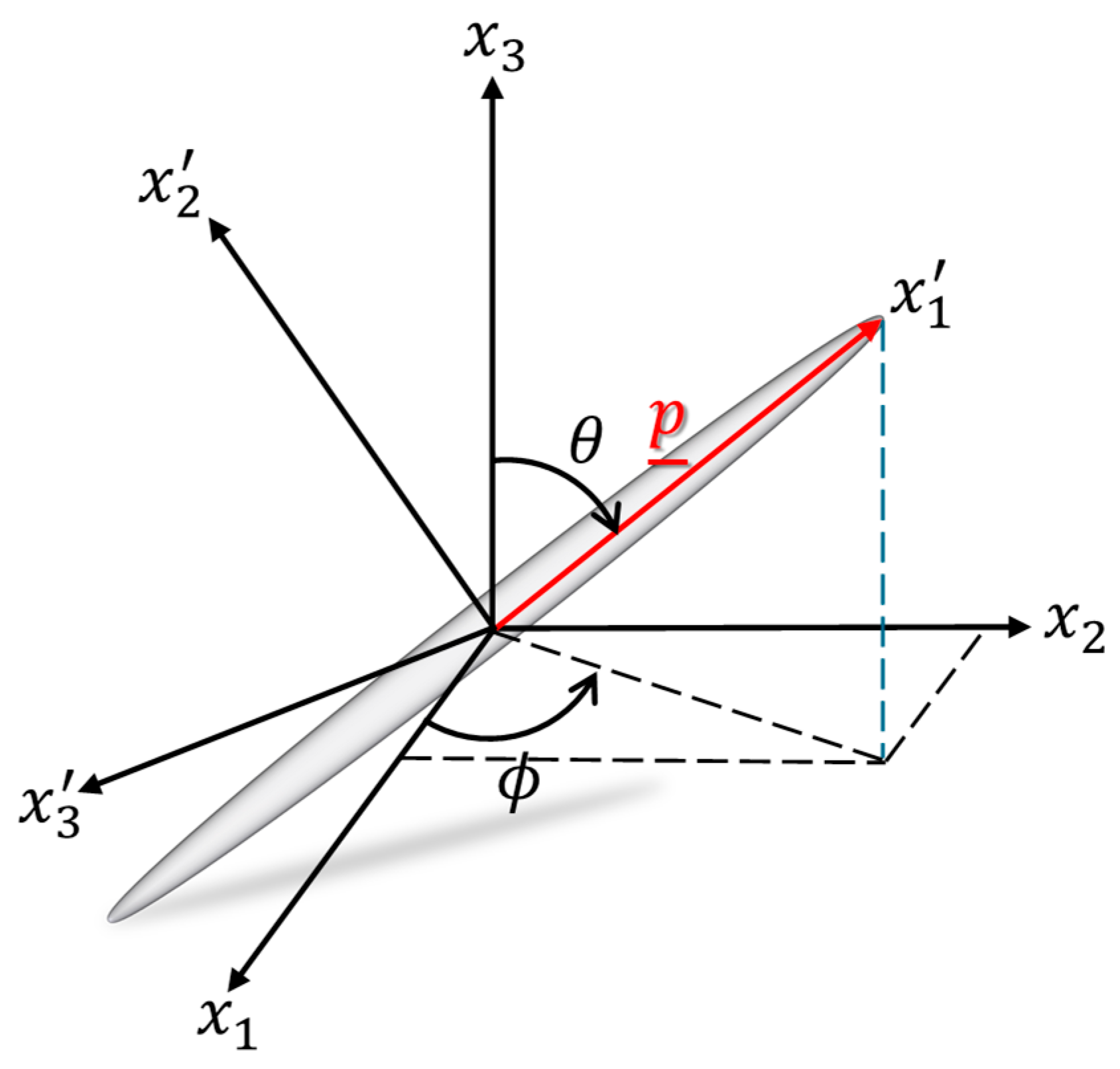
Figure 1. Single ‘rigid’ ellipsoidal fiber orientation.
Jcs 09 00433 g001
Figure 2. Finite difference error e r r 2 for various orientation models and closures (a) over perturbation size δ for the 4th order central difference approximation and for (b) finite difference type and order of approximation at their corresponding optimum perturbation size δ .
Jcs 09 00433 g002
Figure 3. Time evolution of the 2nd order orientation tensor for calibrated FT, PT, iARD, pARD, WPT, Dz and MRD models for (a) a 11 component and (b) a 22 component.
Jcs 09 00433 g003
Figure 4. Values of the residual norm for the (a) NR method and (b) RK45 method for the AT, PT, iARD, pARD, WPT, Dz and MRD models.
Jcs 09 00433 g004
Figure 5. Time evolution of the a 11 ,   a 22   a n d   a 13 components of the 2nd order orientation tensor for calibrated AT, SRF, RSC and FT-RPR models for (a) simple shear flow and (b) shearing/stretching combination flow.
Jcs 09 00433 g005
Figure 6. History of the (a) NR residual norm and (b) RK45 absolute maximum material derivative tensor component for the FT, RSC, SRF, and RPR models for the 2 different flow fields (L1 and L2).
Jcs 09 00433 g006
Figure 7. NR residual norm for different initial orientation states a i j 0 and for (a) AT and (b) RSC orientation tensor models.
Jcs 09 00433 g007
Figure 8. Reconstruction of the orientation distribution function (ODF) for the steady-state orientation for fiber interaction coefficients of (a) CI = 1.0 and (b) CI = 0.01.
Jcs 09 00433 g008
Figure 9. Time evolution of a 11 ,   a 22   a n d   a 13 for the iARD-RPR, iARD-RSC, and pARD-RPR models using materials (a) M1, (b) M2, and (c) M3.
Jcs 09 00433 g009
Figure 10. Iteration history of the (a) NR residual norm and (b) RK45 residual norm for the various coupled models and polymer composites.
Jcs 09 00433 g010
Figure 11. Transient simulation results for (a) a 11 and (b) a 12 for the various Hinch and Leal closure approximations and (c) a 11 and (d) a 12 for the fitted closures.
Jcs 09 00433 g011
Figure 12. Iteration history of the NR residual norm for the (a) Hinch and Leal closures and (b) polynomial fitted closure approximations, and iteration history of the RK45 residual norm for the (c) Hinch and Leal closures and (d) polynomial fitted closure approximations.
Jcs 09 00433 g012
Figure 13. Transient responses of the 2nd order orientation tensor evolution for (a) component a 33 and (b) component a 23 , and residual norm history profiles for the (c) NR method and (d) RK45 method. Results are presented for various flow considerations.
Jcs 09 00433 g013
Table 2. Case Study 1 parameters for the FT, Dz, iARD, pARD, WPT, MRD and PT models [23].
C I ARD Parameters
F T 0.0311 -
D z 0.0258 D z = 0.051 , n ^ = 0 0 1
i A R D 0.0562 C M = 09977
p A R D 0.0169 Ω = 0.9868
W P T 0.0504 w = 0.9950
M R D 0.0198 D 1 = 1.0 ,   D 2 = 0.7946 , D 3 = 0.0120
P T - b 1 b 2 b 3 b 4 b 5
1.924 × 10 4 5.839 × 10 3 0.04 1.168 × 10 5 0
Table 3. Computed error × 10 8 for various orientation tensor models using Hinch and Leal closure approximations.
HYB1HYB2ISOLINQDRSF2HL1HL2
AT0.64360.93850.22200.41880.26912.09490.96184.3940
PT0.80880.75490.58370.50030.42441.67760.82413.4809
iARD0.57371.27120.34440.63360.57280.51000.87741.6148
pARD0.71690.54750.27220.24380.41551.48050.98183.6185
WPT0.85631.03860.37730.25250.29261.45430.96323.5284
Dz0.58990.82480.23730.54840.32330.71371.05942.7732
NEM0.64900.93060.40120.43140.16122.10120.98464.4062
pARD-RSC1.00301.33431.30621.05061.36990.53781.34411.6482
iARD-RPR0.56450.69000.34780.36870.52221.07311.03242.0512
Table 4. Computed error × 10 7 for various orientation tensor models using IBF and EBF closure approximations.
NAT1NAT2ORSORTORWORW3
AT0.35570.58120.45730.33510.59940.6496
PT0.30760.39460.33270.25170.56930.5284
iARD0.25120.26630.21290.19340.47620.4213
pARD0.29750.39560.32160.24790.53540.5229
WPT0.30400.40680.34300.26220.57200.5612
Dz0.35320.32760.28050.29200.67040.6010
NEM0.36490.58690.46150.33880.60620.6520
pARD-RSC0.25290.28000.20740.18020.47720.4155
iARD-RPR0.19640.17090.16010.14040.36870.2820
Table 5. Computed error × 10 7 for various orientation tensor models using IBOF and EBOF closure approximations.
IBOFWTZLAR32VSTFFLAR4LAR4
AT6.17484.31475.08003.15674.31884.3101
PT5.64374.02864.71622.94434.04353.9967
iARD4.49423.07763.67822.26623.01153.0665
pARD5.54583.87414.54152.85483.85003.8818
WPT5.64124.03914.72342.93504.04863.9851
Dz6.42264.80105.54543.39244.80164.6691
NEM6.19784.32545.09363.16534.32714.3182
pARD-RSC4.18212.94013.48782.13582.92362.9070
iARD-RPR3.48822.45092.90821.73592.35902.4110
Table 6. Error estimates of the a 11 ,   a 22   a n d   a 13 steady-state orientation tensor component values for FT, Dz, iARD, pARD, WPT, MRD and PT models.
a 11 a 22 a 13
FT0.00150.00030.0000
PT0.00460.00210.0031
iARD0.00090.00060.0000
pARD0.00060.00030.0032
WPT0.00430.00200.0030
Dz0.00210.00110.0021
MRD0.00150.00080.0046
Table 7. Average processor time taken (sec) to compute the steady state orientation values for both numerical techniques and for the various diffusion models.
FTPTiARDpARDWPTDzMRD
NR0.72100.40750.59160.37840.30380.46150.7908
RK453.58293.97753.00672.64412.77913.44866.7519
Table 8. Case Study 2 parameters for the FT, SRF, RSC and RPR models [10].
A T S R F R S C R P R
C I 0.01 0.01 0.01 0.01
0.1 0.1
α 0.9
β 0
Table 9. Calculated a 11 ,   a 22   a n d   a 13 steady-state error values for RSC, AT, SRF, and RPR models and for the 2 flow fields L1 and L2.
L1L2
a 11 a 22 a 13 a 11 a 22 a 13
RSC0.03740.00580.00000.01780.01220.0017
FT0.00360.00050.00000.00150.00110.0000
SRF0.03740.00550.00240.01580.01090.0050
RPR0.03740.00580.00000.01780.01220.0017
Table 10. ARD-RSC parameters [10] for (a) M1—40 wt. % glass-fiber/PP; (b) M2—31 wt. % carbon-fiber/PP; and (c) M3—40 wt. % glass-fiber/nylon.
M1M2M3
1/301/301/20
b 1 3.842 × 10 4 3.728 × 10 3 4.643 × 10 4
b 2 1.786 × 10 3 1.695 × 10 2 6.169 × 10 4
b 3 5.250 × 10 2 1.750 × 10 1 1.900 × 10 2
b 4 1.168 × 10 5 3.367 × 10 3 9.650 × 10 4
b 5 5.000 × 10 4 1.000 × 10 2 7.000 × 10 4
Table 11. Coupled iARD-RPR and pARD-RPR model parameters [10] for (a) model M1: 40 wt. % glass-fiber/PP, (b) model M2: 31 wt. % carbon-fiber/PP, and (c) model M3: 40 wt. % glass-fiber/nylon.
M1M2M3
C I 0.01650.06300.0060
C M 0.99901.01000.9000
Ω 0.98800.96500.9000
α 0.96500.96500.9500
β 0.00000.00000.0000
Table 12. Calculated errors for a 11 ,   a 22   a n d   a 13 steady-state values for iARD-RPR, iARD-RSC, and pARD-RPR models and materials M1, M2 and M3.
iARD-RPRpARD-RPRiARD-RSC
M1M2M3M1M2M3M1M2M3
a 11 0.10390.07570.08760.08780.02780.09710.11070.03950.3231
a 22 0.05500.02550.02190.04440.01310.02450.05530.02020.0678
a 13 0.12860.17030.04010.06560.02700.04150.08720.04500.0235
Table 13. Calculated error for a 11 ,   a 22   a n d   a 12 steady-state values for (a) Hinch and Leal closure approximations and (b) fitted closure approximations.
(a)(b)
a 11 a 22 a 12 a 11 a 22 a 12
HYB10.00420.00160.0000IBOF0.00680.00000.0000
HYB20.00000.00000.0000ORS0.00000.00000.0000
ISO0.00000.00000.0000ORT0.00610.00130.0000
LIN0.00000.00000.0000NAT10.00000.00000.0000
QDR0.00000.00000.0000ORW0.00670.00000.0000
SF20.00550.00000.0000NAT20.00720.00000.0000
HL10.00420.00140.0000WTZ0.00600.00000.0000
HL20.00380.00000.0000LAR320.00660.00000.0000
ORW30.00660.00000.0000
VST0.00660.00000.0000
FFLAR40.00620.00130.0000
LAR40.00660.00000.0000
Disclaimer/Publisher’s Note: The statements, opinions and data contained in all publications are solely those of the individual author(s) and contributor(s) and not of MDPI and/or the editor(s). MDPI and/or the editor(s) disclaim responsibility for any injury to people or property resulting from any ideas, methods, instructions or products referred to in the content.