Inspection of Damaged Composite Structures with Active Thermography and Digital Shearography

Abstract

This study comprehensively compares the performance of two non-destructive testing (NDT) techniques—active thermography (AT) and digital shearography (DS)—for identifying various damage types in composite structures. Three distinct composite specimens were inspected: a carbon-fiber-reinforced polymer (CFRP) plate with flat-bottom holes, an aluminum honeycomb core sandwich plate with a circular skin-core disbond, and a CFRP plate with two low-energy impacts damage. The research highlights the significant role of post-processing methods in enhancing damage detectability. For AT, algorithms such as fast Fourier transform (FFT) for temperature phase extraction and principal component thermography (PCT) for identifying significant temperature components were employed, generally making anomalies brighter and easier to locate and size. For DS, a novel band-pass filtering approach applied to phase maps, followed by summing the filtered maps, remarkably improved the visualization and precision of damage-induced anomalies by suppressing background noise. Qualitative image-based comparisons revealed that DS consistently demonstrated superior performance. The sum of DS filtered phase maps provided more detailed and precise information regarding damage location and size compared to both pulsed thermography (PT) and lock-in thermography (LT) temperature phase and amplitude. Notably, DS effectively identified shallow flat-bottom holes and subtle imperfections that AT struggled to clearly resolve, and it provided a more comprehensive representation of the impacts damage location and extent. This enhanced capability of DS is attributed to the novel phase map filtering approach, which significantly improves damage identification compared to the thermogram post-processing methods used for AT.

1. Introduction

Aerospace, automotive, and renewable energy industries, among others, rely heavily on non-destructive testing (NDT) to ensure structural integrity. Indeed, the pursuit of non-invasive and NDT techniques for early detection of damage and defects in composite structures remains a central focus of contemporary structural health monitoring (SHM). Such damage and defects can severely impact the load-bearing capacity of a structure and ultimately compromise its integrity. NDT techniques are particularly relevant for inspecting large composite structures such as aircraft wings, fuselage, and other subsurface structural elements.

Both defects and damage negatively impact the ability of a structure to bear loads. Their classification, however, hinges on their source and time. Defects are imperfections or irregularities that arise during various stages of material processing or manufacturing of a structure. Damage, on the other hand, describes the degradation or deterioration that develops during the service life of a structure, which can be induced by applied loads, environmental conditions, or even initiated by an existing structural defect [1]. Composite materials can suffer damage of different sizes and complexities. We can generally group the type of damage into three main levels of severity. The smallest damage encompasses nano-scale damage, which could be very difficult to detect. Simple or primary damage occupies micro-scale to meso-scale levels. These include matrix cracking (tiny cracks in the material’s binding resin), fiber splitting (cracks running along individual fibers or bundles), debonding fiber to matrix (separation between fibers and the resin), microbuckling and waviness in fibers (small, localized buckling of fibers under compression), fiber breakage or fracture (actual breaks in the load-carrying fibers), and kink bands (severe, localized bands of buckled and fractured fibers). The final level involves complex, macro scale damage that can be observed with the naked eye. Unfortunately, most of this damage appears beneath the surface, disabling its visual detection. This level includes delamination (separation of layers within the composite, significantly weakening it), stiffness loss (a noticeable drop in the material’s overall rigidity, indicating extensive internal damage), and impact damage (often hidden, involving a complex mix of internal delaminations, matrix cracking, and fiber breakage caused by external force) [2]. Delaminations and disbonds are the most frequently identified and structurally significant types of damage. Impact damage is also highly critical, largely due to its often-hidden nature and the severe, complex internal flaws it creates [1]. For the inspection of damage in composite structures, the predominant NDT techniques employed include acoustic emission, ultrasonic testing, infrared thermography, terahertz testing, shearography, digital image correlation, X-ray, and neutron imaging [2].

For this work, infrared active thermography (AT) and digital shearography (DS) were chosen due to their significant advantages. These non-contact, full-field optical techniques ensure safe operation in detecting both surface and subsurface damage and defects. They are both the most prevalent optical techniques actively employed for the in-field aircraft inspection and are often stipulated in composite component inspection manuals. AT is an optical imaging technique that makes use of thermal waves. The basis of thermal imaging lies in detecting the infrared radiation emitted by the inspected surface of the specimen [3]. While often approximated as an ideal blackbody for analytical simplicity, real materials emit radiation proportional to their absolute temperature and their emissivity. Indeed, unlike an ideal blackbody, whose emission depends solely on temperature, the emissivity of real materials varies with factors like material type, surface finish, and wavelength [4]. The sensor unit responsible for receiving and integrating this emitted radiation is typically a bolometer. Modern infrared cameras integrate a rectangular array of elementary bolometers with specialized lenses, commonly made of Germanium or Zinc-selenide. These materials are transparent to infrared wavelengths (while blocking visible light), forming an optical system crucial for infrared image formation [3]. Such systems are designed to record the thermal response with high spatial, temporal, and thermal resolution. An external heat source is commonly used to generate thermal waves that propagate through the thickness of the specimen. If these waves encounter anomalies in the material, they will exhibit a distinct reflection pattern. This pattern results in a temperature variation at the surface that is then captured by an infrared camera. DS is a laser-based optical interferometric method used to measure surface strains resulting from external stimuli such as thermal, vacuum, or vibrational loads [5]. It uses an optical configuration more resilient to environmental disturbances and vibrations than other interferometric techniques and has become an important diagnostic tool in nondestructive testing [6]. A camera captures the intensity pattern generated by laser speckle interference. When the specimen is subjected to an external load, small deformations are produced on its inspected surface. These deformations are captured by the camera as variations in the intensity patterns. Subsurface damage often leads to the appearance of regions of higher deformation, which indicates the presence of internal flaws like delaminations, cracks, or bond failures.

Hung et al. [7] wrote a comprehensive review of AT and DS techniques, delineating their advantages and limitations. The work directly compares the results yielded by thermal pulse excitation on composite, metallic, and plastic specimens. DS and AT with different excitation sources were used by Georges et al. [8] for the inspection of hybrid composite-metal sandwich structures made of titanium skins and CFRP/GFRP mix core. Both techniques yield good results, and it is suggested that they can be used as separate techniques or under integrated schemes. Wei et al. [9] compared long pulse thermography (LPT) and shearography for defect evaluation. This research focused on detecting disbonding defects in rubber-to-metal and aluminum sandwich plates, as well as flat-bottom hole defects in carbon-fiber reinforced polymer (CFRP) panel. The authors determined that LPT and DS are complementary techniques. They observed that LPT performed best in identifying disbonds in rubber-to-metal plates and flat-bottom holes in CFRP panels, whereas DS proved to be more effective for disbond identification in aluminum sandwich plates. Notably, LPT demonstrated a significantly lower error than DS for damage size evaluation. A crucial insight was also the critical role of post-processing methods in improving the defect identification for both techniques. Very recently, Ochana et al. [10] assessed the effectiveness of AT and DS as non-destructive NDT technique for 3D-printed thermoplastic (TP) composites reinforced with continuous carbon fiber. Artificial defects of varying sizes and depths were introduced for benchmark purposes. AT identified defects by observing surface temperature changes. It proved effective for defects up to 1.25 mm deep (and some at 1.5 mm), enhancing their presence through thermal anomalies. However, its limitations included difficulty in detecting deeper or smaller defects and accurately determining their shapes due to thermal diffusion effects. DS successfully identified near-surface defects within the same size range. While effective for these, it required greater expertise for accurate interpretation and, like AT, it struggled with detecting smaller and deeper imperfections.

The present study compares the efficiency of AT and DS, along with their respective post-processing techniques, for identifying various types of damage in three distinct composite specimens: a carbon-fiber-reinforced polymer (CFRP) plate containing multiple flat-bottom holes, an aluminum honeycomb core sandwich plate featuring a circular skin-core disbond, and a CFRP plate presenting two low-energy impacts damage.

2. Materials and Methods

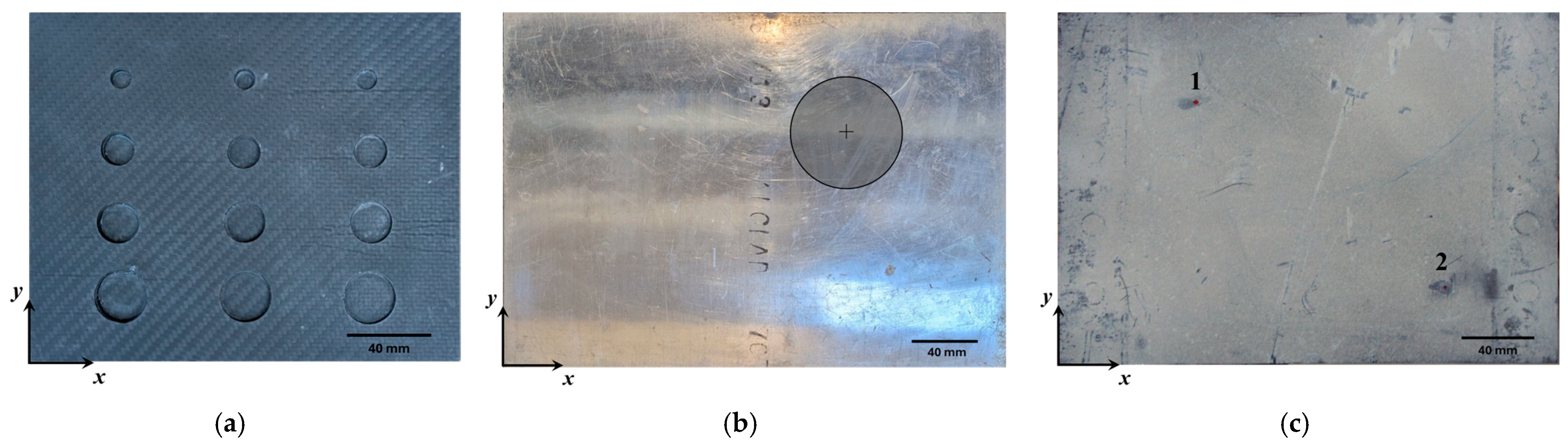
2.1. Inspected Structures

This study aims to compare the effectiveness of two NDT techniques, active thermography (AT) and digital shearography (DS), in identifying different types of damage in composite structures. For this purpose, three plate specimens were inspected. Specimen 1 is a CFRP plate with several flat-bottom holes; specimen 2 is an aluminum honeycomb core sandwich plate with a circular core-skin disbond; and specimen 3 is a CFRP plate with two low-energy impacts damage. These three composite structures were selected for their relevance in the aerospace, automotive, and renewable energy industries. For instance, sandwich structures can be found in a great variety of aircraft [11], a huge amount of CFRP is replacing metal components in space launchers [12], CFRP structures appear in several parts of cars [13], and the materials commonly used in wind turbine blades are fiber reinforced polymers [14]. Composite structures are particularly susceptible to several types of damage such as delamination, matrix cracking and crushing, fiber breakage, and debonding [15,16,17,18,19,20,21]. The three chosen specimens present distinct damage types: the flat-bottom holes in specimen 1 mimic multiple delaminations of various sizes and depths in plates [22,23]; the missing adhesive in the second specimen simulates debonding between the core and the skin [18]; and finally, specimen 3 is subjected to low-energy impacts of 13.5 J and 26.2 J in order to create barely visible impact damage (BVID).

Specimen 1 was made from a single laminated plate consisting of seven layers of prepreg woven carbon fiber/epoxy. The stacking sequence of (45/0/45/0/45/0/45) was chosen to provide nearly isotropic mechanical properties. The fabrication of the plate with flat-bottom holes involved three steps. Initially, the single laminated plate was cut into four equal parts. Subsequently, through-holes of varying dimensions were drilled into three of these parts. Finally, these four parts were glued together using epoxy resin, forming a consolidated plate with the distinct bottom hole configurations. Figure 1a presents a photo of specimen 1 showing the flat-bottom holes on the back surface. The plate has overall dimensions of 206 mm (length) × 170 mm (width) × 8 mm (thickness). Its design incorporates three vertical columns, each containing four flat-bottom holes. The flat-bottom holes decrease in diameter with the y coordinate: 25 mm, 20 mm, 16 mm, and 10 mm. The depth of the flat-bottom holes also varies with the x coordinate: 6 mm, 4 mm, and 2 mm. The second specimen consists of an aluminum sandwich plate, comprising a honeycomb core, with 4.33 mm cell dimensions, and two skins, each 0.8 mm in thickness. The overall plate dimensions are 315 mm in length, 220 mm in width, and 12 mm in thickness. An artificial circular debond, 70 mm in diameter, was deliberately introduced during manufacturing by removing the adhesive that bonds the honeycomb core to one of the skins. This flaw simulates a lack of adhesion between the honeycomb core and one of the skins, and is located at coordinates (215 mm, 150 mm). Figure 1b presents a photo of the front surface of specimen 2, highlighting the location and size of the circular damage. Specimen 3 is a CFRP rectangular plate, measuring 276.5 mm in length, 198 mm in width, and 1.825 mm in thickness, with a stacking sequence of (0/90/+45/−45/0/90)_S and containing two internal damaged areas [24]. Internal damage was generated within the plate by two low-energy impacts. These impacts consisted of dropping a 62.2 mm diameter steel sphere onto the plate. The first impact occurred at coordinates (74 mm, 147 mm) with an energy of 13.5 J and the second at (215 mm, 38 mm) with an energy of 26.2 J. It can be pointed out that according to AIRBUS standards, the impact energy threshold for generating a BVID is 50 J [25]. The plate surface was coated with a thin white powder to aid in identifying the two impact locations. Figure 1c shows a photo of the front surface of specimen 3 after the impacts, where the only visible effect was the absence of white powder in the contact points of the sphere with the plate.

2.2. NDT Techniques Employed in Inspection

The following two sections describe the NDT techniques used for inspection of the three specimens. The first, AT, uses an external heat source to generate a thermal wave through the thickness; an infrared camera then monitors surface temperature changes over time to reveal hidden damages. The DS technique, on the other hand, employs a laser illumination and an optical interferometer to capture the evolution of surface deformation gradients, often induced by an external heat source, thereby identifying areas of strain concentration indicative of damage.

2.2.1. Active Thermography (AT)

The first NDT technique used to identify damage is AT, which can be subdivided according to the kind of applied thermal excitation [26,27]. In the present work, two types of AT were used in the inspection of specimens: (1) pulsed thermography (PT) and (2) lock-in thermography (LT). In PT, a rectangular pulse thermal stimulation is delivered to the inspected surface, whereas in LT the stimulation is harmonic. Figure 2 shows the experimental setup used in this study. For specimen 1, the inspection was performed on the surface opposite the one containing the flat-bottom holes. For the other specimens, the inspections were on the outer surface of the disbonded skin of specimen 2, and on the impacted surface of specimen 3.

The thermal images, or thermograms, of the inspected surfaces were recorded using a FLIR^® A6751sc infrared camera. This camera has a 640 × 512 pixel resolution and is sensitive to infrared radiation in the 3–5 µm spectral band. The thermal excitation was supplied by two 2 kW halogen lamps from Automation Technologies^®, powered by an IRX-Box. The National Instruments^® NI USB-6251 module provided synchronization between the acquisition of thermograms and the thermal loading. Before the tests, the inspected surfaces were coated with a thin matte black paint to reduce emissivity variations and minimize reflectivity. The specimens were positioned vertically, supported at their lowest bottom corners, and the surface aligned with the camera’s optical axis. Two halogen lamps were placed symmetrically around the inspected surfaces at approximately a 45-degree angle and a distance of 50 cm to ensure nearly uniform thermal loading.

Figure 3a shows schematically the sequential acquisition of several thermograms and Figure 3b illustrates typical temperature evolutions at a given pixel located at coordinates $(x, y)$ measured with both AT variants. For measurements with the PT variant, a transient 4 kW excitation was applied to the inspected surfaces, and thermograms were acquired at 7.5 fps just after the thermal excitation. The LT variant involved applying a harmonic wave of two period duration of 2 kW amplitude, being the thermograms acquired at 60 fps during the thermal loading. The thermal loading parameters for achieving the best damage identification results were found by testing various rectangular pulse durations and harmonic frequencies. The optimal parameters for PT pulse duration and LT harmonic excitation were found to be: 12 s and 0.008 Hz for specimen 1; 0.3 s and 0.111 Hz for specimen 2; and 0.5 s and 0.125 Hz for specimen 3, respectively. It should be highlighted that the results are linearly converted into an 8-bit grayscale image for a clear and intuitive visualization of their distribution. This conversion yields a high-contrast representation, thereby facilitating the rapid identification of subtle, damage-induced differences.

2.2.2. Digital Shearography (DS)

The second NDT technique presently applied for the identification of damage in the three composite structures is DS with thermal loading. An in-house built DS system, based on a Michelson interferometer and employing temporal phase modulation, was used to monitor the deformation of the specimens during the cooling stage after applying a thermal load. The experimental setup for these measurements is presented in Figure 4. All the devices and the inspected specimens are mounted on top of an optical table with pneumatic suspension to minimize the influence of external vibrations during data acquisition. The specimens were held vertically, secured to the optical table by two supports at their lowest bottom corners. Measurements were carried out on the same surfaces of the specimen, previously inspected by thermography. The inspected surfaces were covered by a thin layer of white power to create a uniform reflection of the laser light. These surfaces are illuminated uniformly by a 532 nm continuous wave (CW) laser from Coherent (Verdi)^®. The DS system generates an interference pattern from the reflection wave, and a 4000 × 3000 pixels digital camera from Basler (acA4112-20um) ^® captures its intensity. Temporal phase modulation of four images with a phase step π/2 is then used to extract the phase of the interference pattern [28]. This modulation requires the translation of a Michelson interferometer mirror using integrated piezoelectric transducers, actuated by a piezoelectric controller. A 5 mm shearing amount was simultaneously applied in both the x and y directions by slightly tilting the second mirror of the Michelson interferometer. The experimental procedure began with the application of a 10 s rectangular thermal pulse to the inspected surface, using a 500 W halogen lamp. Subsequently, during the 96 s cooling stage of the plate, four images, each corresponding to a phase step of 0, π/2, π, and 3π/2, were acquired at 8 s intervals. The acquisition time for each image set was approximately 0.4 s. These images were stored in a computer for later computation of the interference phase. The evaluation of phase maps for each interval, which are directly related to the relative deformation of the inspected surface, involves correlating the interference phases of two consecutive records. In other words, the phase map $\mathsf{\Delta }\varphi \left(x,y,t+\Delta t\right)$, at an instant $t+\mathsf{\Delta }t$, is the subtraction between two consecutive interference phases $\mathsf{\Phi }\left(x,y,t+\Delta t\right)$ and $\mathsf{\Phi }\left(x,y,t\right)$, where $\mathsf{\Delta }t$ is a predefined time step. In the present study, 13 interference phases were acquired, resulting in 12 phase maps.

2.3. Damage Identification Procedure

Identifying structural damage by analyzing the global structural response is challenging because damage typically induces small and localized variations that are difficult to differentiate from the response of the structure in the undamaged state. To enhance damage detectability, it is necessary to post-process the experimental raw data using dedicated tools to extract these damage-induced variations. The following subsections describe the tools and procedures used for damage identification, applied to thermograms from thermography and phase maps from digital shearography.

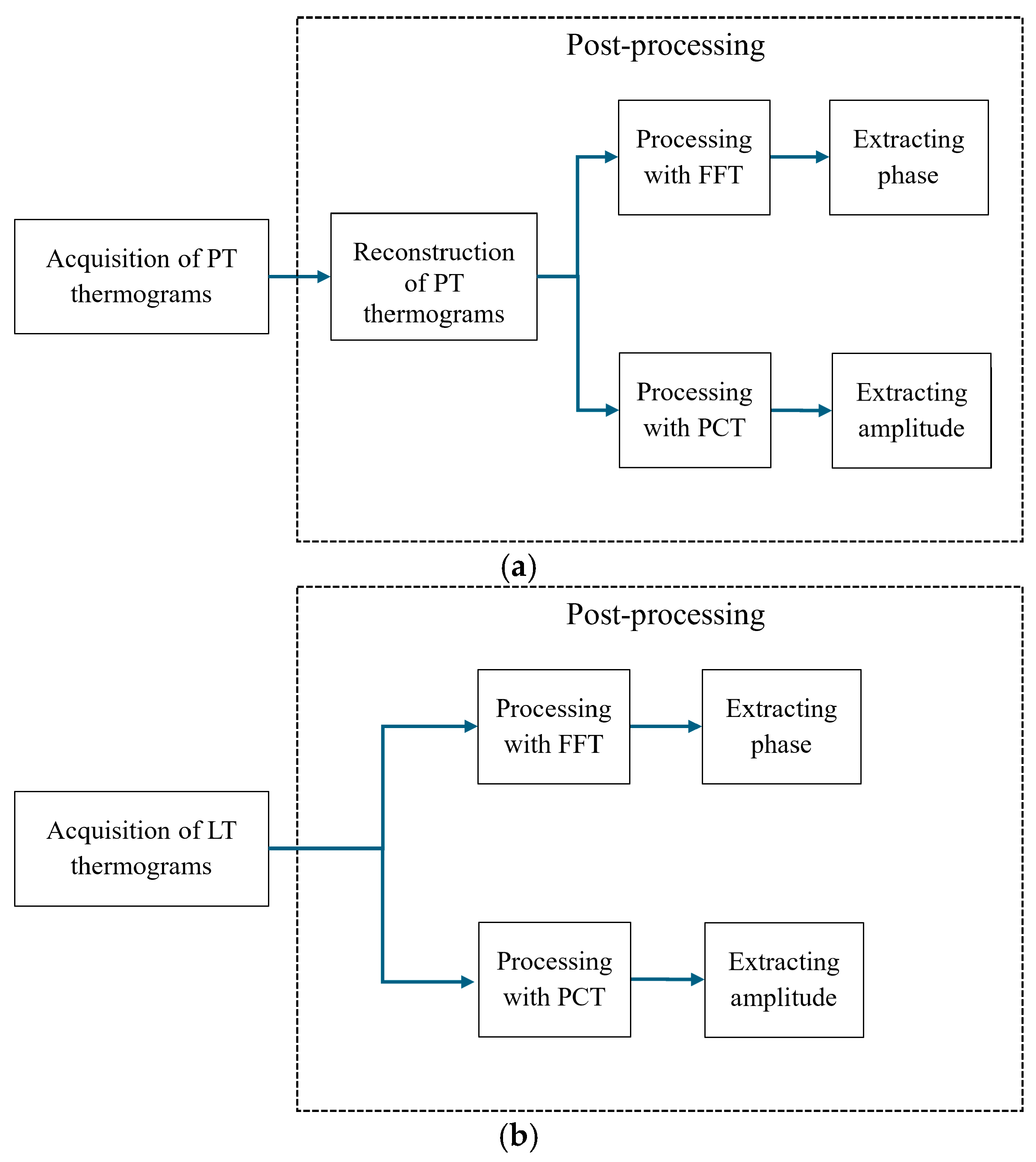
2.3.1. Post-Processing of Thermograms

The need for thermograms post-processing is illustrated in Figure 5, which shows raw thermograms acquired with PT and LT. It is clear that the damage is only visible in the deeper flat-bottom holes, i.e., the holes on the right column.

In PT, thermographic signal reconstruction (TSR) is frequently applied to improve the quality of thermograms. Typically, TSR involves fitting a 4th or 5th-degree polynomial to the logarithmic temporal decay of the thermal signal at each pixel. This procedure effectively attenuates temporal noise from the IR camera and mitigates artefacts caused by reflection and air convection, resulting in time-filtered thermograms [29]. Basically, TSR is based on approximating the logarithmic time dependence of a pixel in a thermogram by an $M$th-degree polynomial

$$\mathrm{l}\mathrm{n}\left[T\left(t\right)\right]=\sum _{k=0}^M{a_k\left[ln\left(t\right)\right]}^k$$

(1)

and reconstructing the original thermographic signal according to

$$T\left(t\right)=\mathrm{e}\mathrm{x}\mathrm{p}\left(\sum _{k=0}^M{a_k\left[ln\left(t\right)\right]}^k\right)$$

(2)

where $T$ and $t$ stands for temperature and time, respectively, with $a_k$ being the polynomial coefficients.

The fast Fourier transform (FFT) is applied to a temporal sequence of thermograms to compute phase in the temperature [30]. In PT, the temporal evaluation of the temperature phase is accomplished by applying a FFT to a sliding set of 15 thermograms. On the other hand, in LT, only a single temperature phase is extracted by applying a FFT to the full set of thermograms. The sequence of thermograms provides a temperature time series, $\left\{T\left(x,y,t_0\right), T\left(x,y,t_1\right), T\left(x,y,t_2\right), \cdots ,T\left(x,y,t_{N_T-1}\right)\right\}$, for each pixel located at coordinates $(x,y)$. The length of this series, $N_T$, corresponds to the number of acquired thermograms. The FFT algorithm efficiently computes the discrete Fourier transform (DFT), which is then applied to the temperature profiles extracted from thermograms. This process transforms these temperature profiles $T(x,y,t)$ into the frequency domain, where each frequency component $F_k(x,y)$ is given by the DFT equation:

$$F_k\left(x,y\right)={\displaystyle \frac{1}{N_T}}\sum _{n=0}^{N_T-1}T\left(x,y,t_n\right) e^{-{\displaystyle \frac{i2\pi kn}{N_T}}}$$

(3)

where $i$ represents the imaginary unit and $F_k(x,y)$ is a complex number that contains both magnitude and phase information for the frequency order $k$. The magnitude $\left|F_k\right(x,y\left)\right|$ and phase ${\varphi }_k(x,y)$ are then extracted according to:

$$\left|F_k\left(x,y\right)\right|=\sqrt{{\left[Re\left(F_k\left(x,y\right)\right)\right]}^2+{\left[Im\left(F_k\left(x,y\right)\right)\right]}^2,}$$

(4)

$${\varphi }_k\left(x,y\right)=\mathit{atan}\left[{\displaystyle \frac{Im\left(F_k\left(x,y\right)\right)}{Re\left(F_k\left(x,y\right)\right)}}\right]$$

(5)

respectively. The magnitude and phase spectra are obtained by computing each frequency component from order $0$ through $N_T/2$. For each pixel with coordinates $(x,y)$, the specific temperature phase is retrieved from the frequency component with the highest magnitude in its respective spectrum.

Principal component thermography (PCT) [31,32] is a method applied to thermal data to extract the most valuable information, especially when looking for damage. PCT can be interpreted as an eigenvalue and eigenvector decomposition of the thermal data covariance matrix. This decomposition is usually carried out by using the singular value decomposition (SVD) algorithm. SVD is highly favored because it offers superior numerical stability and efficiency, particularly when dealing with large datasets such as the ones found in thermography. The procedure begins by reorganizing the thermogram sequence, initially a 3D matrix. These data are reshaped into a single 2D matrix, often denoted as $\mathbf{D}$. In this matrix, each row represents all pixel values from a single time instant, while each column corresponds to a specific time instant within the sequence. The next step involves centering the temperature for each instant (column) by subtracting the average temperature to all elements in matrix D, creating a centered temperature matrix, ${\mathit{D}}_c$. This matrix is then decomposed using SVD, expressed as

$${\mathit{D}}_c=\mathbf{U}\mathsf{\Sigma }{\mathbf{V}}^T,$$

(6)

where $\mathbf{U}$ contains the left singular vectors, interpreted as spatial basis principal components, $\mathsf{\Sigma }$ is a diagonal matrix containing the singular values, which are related to the eigenvalues of the covariance matrix, and $\mathbf{V}$ is the right singular vectors, representing temporal basis principal components scores. The singular values in $\mathsf{\Sigma }$ are arranged in decreasing order, indicating the relative importance or contribution of each principal component. The first component typically represents the global thermal response, whereas the components from the second to around the tenth order are generally used to reveal thermal anomalies induced by the damage. Higher-order components are typically discarded as they are predominantly associated with experimental noise. The thermograms are reconstructed using only the selected temporal basis principal components ${\mathbf{V}}_{\mathbf{s}}$. The selection of the principal components was based on the visualization of the thermal image of each component. This process effectively retains the dominant thermal patterns while reducing noise and less significant variations. To achieve this, we first compute the principal component scores matrix PS by projecting the centered temperature matrix ${\mathit{D}}_c$ onto the selected principal components ${\mathbf{V}}_{\mathbf{s}}$:

$$\mathbf{P}\mathbf{S}={\mathit{D}}_c\cdot {\mathit{V}}_s.$$

(7)

Then, these scores are multiplied by the transpose of the selected principal components, transforming the data back into the original temperature space and resulting in the filtered thermograms ${\mathit{D}}_f$:

$${\mathit{D}}_f=\mathbf{P}\mathbf{S}\cdot {\mathit{V}}_s^T.$$

(8)

The last step involves reshaping the 2D matrix of the filtered thermograms into a 3D matrix, thus reconstructing the thermogram time sequence. The flowchart in Figure 6a illustrates the post-processing procedure for PT. Initially, the PT thermograms are time-filtered by TSR to attenuate noise and mitigates artefacts. The TSR-processed thermograms are post-processed using FFT and PCT to extract the phase and amplitude, respectively. On the other hand, we see in Figure 6b that the phase and the amplitude of LT thermograms are extracted directly by FFT and PCT.

2.3.2. Post-Processing of Phase Maps

A DS system produces phase maps, showing how a deformation gradient or slope of a structure changes between two specific moments. The values in these phase maps are wrapped between $[-\pi ,\pi ]$ (or $\left[\mathrm{0,2}\pi \right]$) due to the need of computing the inverse tangent function to extract the interference phase from a series of recorded intensity images [33]. This wrapping is characterized by abrupt phase discontinuities across the map, commonly known as fringes. In addition, the presence of experimental noise, primarily due to speckle decorrelation, contaminates these phase maps. This noise diminishes the clarity of phase values and fringe visibility, thereby making it difficult to interpret the surface deformation gradient. Figure 7 displays a raw phase map of specimen 1. While it shows four distinct vertical fringes and a subtle phase variation along the right fringe, it does not reveal the flat-bottom holes. This demonstrates that post-processing of raw phase maps is essential for extracting damage-induced features and improving damage detectability.

The most common post-processing procedure is filtering and unwrapping the phase maps, thus reducing noise and eliminating the discontinuities in the raw phase map [9,15,22,23,24,33]. However, this improvement may not be substantial if the damage is relatively small. In such cases, another step in the post-processing is to differentiate the continuous filtered and unwrapped phase map [24,33]. However, besides the significant computational effort that this type of post-processing requires, it is difficult to achieve a crucial balance between preserving damage-induced high-frequency signal components and filtering out high-frequency experimental noise. This work employs, for the first time, a simpler, more direct, and very efficient procedure: the application of a band-pass filter to reveal the essential damage-induced phase variations in the maps, which are then summed across different time instants for enhanced visibility.

Typically, low-pass filters are applied to raw phase maps to reduce high-frequency experimental noise while preserving the relevant phase information. However, to effectively handle the cyclic nature of phase and its discontinuities before applying the low-pass filter, the phase maps are often first transformed into their complex exponential representation. This allows the filtering to be performed in the complex domain, which intrinsically deals with the $2\pi$ phase wraps and better preserves true phase variations. The raw phase map ${\Delta \varphi }_r(x,y,t)$, evaluated at a generic instant $t$, is converted to the complex map $Z_r(x,y,t)$ using Euler’s formula:

$$Z_r\left(x,y,t\right)=e^{i\Delta {\varphi }_r\left(x,y,t\right)}=\mathit{cos}\left({\Delta \varphi }_r\left(x,y,t\right)\right)+i\mathit{sin}\left({\Delta \varphi }_r\left(x,y,t\right)\right).$$

(9)

A moving average filter, which acts as a low-pass filter, is applied to the complex map $Z_r(x,y,t)$ in the spatial domain using a 2D convolution, with the filtered complex map $Z_f(x,y,t)$ given by:

$$Z_f\left(x,y,t\right)=Z_r\left(x,y,t\right)\ast h(M,N),$$

(10)

where the symbol $\ast$ represents the convolution operator, $h(M,N)$ is the window, and $M$ and $N$ denote the vertical and horizontal dimensions of this window, respectively. The filtered phase map, ${\Delta \varphi }_f(x,y,t)$, is retrieved by applying the arctangent function to the imaginary and real components of the filtered complex map $Z_f(x,y,t)$:

$${\Delta \varphi }_f\left(x,y,t\right)=\mathrm{a}\mathrm{t}\mathrm{a}\mathrm{n} \left[{\displaystyle \frac{Im\left(Z_f\left(x,y,t\right)\right)}{Re\left(Z_f\left(x,y,t\right)\right)}}\right].$$

(11)

The process described by Equations (9)–(11) can be repeated for a specified number of passes to further attenuate the experimental noise. The cutoff frequency of the filter is directly related to both the window size and the number of passes. To generate two filtered phase maps, ${\Delta \varphi }_{lcf}\left(x,y,t\right)$ and ${\Delta \varphi }_{hcf}\left(x,y,t\right)$, the process described above is applied twice. The first phase map ${\Delta \varphi }_{lcf}\left(x,y,t\right)$ corresponds to a filter with lower cutoff frequency, whereas the second ${\Delta \varphi }_{ucf}\left(x,y,t\right)$ is obtained with a filter having a higher cutoff frequency. These two phase maps are then subtracted and corrected, yielding a final filtered phase map:

$${\Delta \varphi }_{b-p}(x,y,t)=\left\{\begin{array}{c}\begin{array}{ll}\left[{\Delta \varphi }_{ucf}\left(x,y,t\right)-{\Delta \varphi }_{lcf}(x,y,t)\right]-2\pi & if \left[{\Delta \varphi }_{ucf}\left(x,y,t\right)-{\Delta \varphi }_{lcf}(x,y,t)\right]>\pi \\ \left[{\Delta \varphi }_{ucf}\left(x,y,t\right)-{\Delta \varphi }_{lcf}(x,y,t)\right]+2\pi & if \left[{\Delta \varphi }_{ucf}\left(x,y,t\right)-{\Delta \varphi }_{lcf}(x,y,t)\right]<-\pi \\ \left[{\Delta \varphi }_{ucf}\left(x,y,t\right)-{\Delta \varphi }_{lcf}(x,y,t)\right]& otherwise\end{array}\end{array}\right.$$

(12)

The result of subtracting the phase maps is equivalent to applying a band-pass filter, as ${\Delta \varphi }_{b-p}(x,y,t)$ contains only information in the frequency band between the lower and higher cutoff frequencies. Notice that the subtraction and correction yield a continuous map and thus there is no need to unwrap it. Finally, the band-pass filtered phase maps from different time instants are summed to enhance the visibility of phase variations indicative of damage features:

$${\Delta \varphi }_s\left(x,y\right)=\sum _{k=1}^{N_{\Delta \varphi }}{\varphi }_{b-p}\left(x,y,t_k\right),$$

(13)

where $N_{\Delta \varphi }$ is the total number of band-pass filtered phase maps that were acquired. A last step consists of converting ${\Delta \varphi }_s\left(x,y\right)$ to a grayscale image for a clearer visualization of the phase distribution. The flowchart in Figure 8 depicts the post-processing methodology applied to the acquired phase map data. This procedure comprises three primary operations: defining the band-pass filter cutoff frequencies, sequential processing of the phase maps, and summing the band-pass filtered phase maps. The phase map band-pass filter is implemented by subtracting the phases processed through two low-pass filters with different cutoff frequencies. The selection of these frequencies is empirically driven, based on their observed effect on the first phase maps acquired. Specifically, the higher cutoff frequency is set to attenuate only high-frequency speckle noise, while the lower cutoff frequency is chosen to provide a mild smoothing effect, ensuring that critical information in phase maps is preserved, such as phase discontinuities. Following this, the identical band-pass filter is applied to the phase map sequence. Finally, the resulting band-pass filtered phases are then aggregated through their summation.

3. Results

A comprehensive series of experiments and measured data post-processing was conducted. This included adjusting the thermal excitation and acquisition configurations, as well as selecting the most appropriate post-processing parameters. The most successful outcomes are reported in the following two subsections.

3.1. Active Thermography (AT)

This section presents the best damage identification results, namely temperature phase and temperature amplitude, for the three specimens analyzed. These results were obtained through the post-processing of LT and PT thermograms using the TSR, FFT, and PCT methods. First, TSR is applied to LT thermograms by fitting a 5th-degree polynomial to the logarithmic temporal decay curve for each individual pixel, thus extracting more robust and interpretable thermal signatures. Then, from the FFT, temperature phases were extracted at the frequency of highest magnitude, while from the PCT, temperature amplitudes were obtained by selecting components 4 to 10, which were deemed to contain the most relevant information about the damage. Figure 9, Figure 10 and Figure 11 display the temperature phase and amplitude images that most clearly reveal the damage. Their selection was based on an analysis of the results over the entire recorded time.

The inspection results for specimen 1, shown in Figure 9, clearly reveal distinct, localized circular anomalies against a relatively uniform background, indicative of subsurface damage. Three main regions can be identified: (1) the right column displays four circles that increase in size and contrast from top to bottom, corresponding to 6 mm deep holes; the middle column contains two to three smaller and fainter spots, indicating 4 mm deep holes; and (3) the left side reveals very diffuse and almost imperceptible variations where the column of 2 mm deep holes is located. The left side of the PT temperature phase image (Figure 9a) exhibits a mid-gray background with noticeable mottled patterns. This pattern is likely attributable to a non-uniform adhesive layer introduced during the plate fabrication process. Specifically, the PT temperature amplitude image reveals highly contrasted circular anomalies, presenting as both bright and dark features, unlike the diffuse appearances observed in other processed thermograms in Figure 9b–d.

Figure 10 shows the inspection results for specimen 2, which was designed to simulate a circular adhesive debonding between the core and one of the skins. Compared to the previous set of results (Figure 9), the anomalies in these images appear more diffuse and less sharply defined, characteristics attributed to the high thermal diffusivity of the aluminum. This observation aligns with the findings of Wey et al. [9], who similarly reported less distinct results when analyzing the thermal response of an aluminum sandwich plate with artificial debondings. The LT temperature phase image (Figure 10c) is notably darker in its central region compared to its lateral edges and exhibits a greater range of brightness variations than the other images. The PT temperature phase image (Figure 10a) reveals a very faint, diffuse, and slightly lighter oval-shaped anomaly in the upper central-right region. A similar oval-shaped anomaly is also present in the LT temperature amplitude image (Figure 10b), though it appears significantly more prominent and less diffuse. On the other hand, this anomaly is not clearly discernible in the highly contrasted LT temperature phase image (Figure 10c). However, the same oval-shaped anomaly appears significantly more prominent, lighter, and less diffuse in the PT temperature amplitude image (Figure 10b). A small anomaly on the image left edge also shows distinct appearances: it is visible as a darker small area in the PT temperature phase image (Figure 10a), a lighter small area in the PT temperature amplitude image (Figure 10b), and a lighter small area, but less distinct due to the inherently high contrast and varied patterns, in the LT temperature phase image (Figure 10c).

The inspection results for specimen 3 are depicted in Figure 11. The images reveal two distinct anomalies, discernible by their contrast with the surrounding background, which are likely attributable to subsurface damage. Specifically, a large region, containing two contiguous areas with different contrasts and shapes, is consistently observed in the lower right corner, while a small region is visible in the upper-left quadrant of all four images. The areas of these anomalies extend over the precise locations of the two impacts. Furthermore, the energy of each impact correlates with the observed area and contrast level of its corresponding anomaly. A cross-analysis of the images reveals anomalies with distinct contrast. The PT temperature phase image (Figure 11a) presents prominent brighter anomalies against a darker background. On the other hand, the LT temperature phase image (Figure 11c) generally appears brighter and more diffuse, with its anomalies showing significantly less distinct contrast. Meanwhile, the PT temperature amplitude image (Figure 11b) and the LT temperature amplitude image (Figure 11d) both exhibit sharper and more pronounced features than LT temperature phase image (Figure 11c). A particular challenge is consistently identifying the smaller and circular anomaly located in the upper-left quadrant. Its less pronounced contrast, particularly evident in the brighter and more diffuse LT temperature phase image (Figure 11c), makes its precise identification rather difficult.

3.2. Digital Shearography (DS)

The DS technique was used to monitor the deformation gradient of the plate during its cooling stage. This involved recording twelve phase maps, each separated by an 8-s interval. The post-processing procedure of these phase maps involved two steps: first, applying a band-pass filter to highlight the damage-induced anomalies, and then summing the resulting filtered maps to enhance the visibility of these anomalies.

The band-pass filtered phase maps, highlighting damage-induced anomalies, were obtained by subtracting the high-frequency signal component (derived from a low-pass filter with a higher cutoff) from the low-frequency signal component (derived from a low-pass filter with a lower cutoff). These low-pass filters were generated individually by applying multiple passes of a moving average with varying window sizes and number of passes. A larger window size leads to more aggressive smoothing and results in a lower cut-off frequency, which can be further reduced by applying multiple passes. For all measurements, the parameters for the higher cut-off frequency were kept constant, using a window size of 15 × 15 with 8 passes. However, the parameters for the lower cut-off frequency were adjusted based on observation of phase anomalies in the resulting band-pass filtered phase map for each specimen. Specifically, a 175 × 175 window with 10 passes was applied for specimen 1, a 95 × 95 window with 10 passes for specimen 2, and an 85 × 85 window with 10 passes for specimen 3. Figure 12, Figure 13 and Figure 14 display two sets of results for specimens 1, 2, and 3, respectively. For each, these figures show the individual filtered phase maps acquired at 8 s, alongside the sum of all twelve filtered phase maps.

The inspection results for specimen 1, displayed in Figure 12, effectively reveal localized circular image anomalies indicative of subsurface damage. These anomalies are distributed along columns and increase in size and visibility from top to bottom. The individual filtered phase map acquired at 8 s (Figure 12a) clearly displays a single column of circular anomalies on the right side, corresponding to flat-bottom holes with a depth of 6 mm. Conversely, the sum of twelve filtered phase maps (Figure 12b) demonstrates an enhancement in their visibility, revealing two columns of circular anomalies across both the right and middle sides of the plate, corresponding to flat-bottom holes with depths of 6 mm and 4 mm, respectively. Indeed, the image of the sum of filtered phase maps (Figure 12b) provides a much clearer and less noisy representation of the underlying image anomalies than the image of individual filter phase maps (Figure 12a). Even with this enhancement, the anomalies from smaller diameter holes, located on the top of the image, remain less distinct. Furthermore, the column of flat-bottom holes with a depth of 2 mm, located on the left side of the plate, remains undetected. A small anomaly is also observed within the circular feature located in the bottom-left corner. This correlates with a small imperfection visible on the surface of the 6 mm deep flat-bottom hole.

Figure 13 displays the inspection results for the aluminum sandwich plate (specimen 2). Consistent with prior observations in Figure 12, the sum of filtered phase map demonstrates a noticeable enhancement in the visibility of image anomalies compared to an individual filtered phase map. In both images, a circular anomaly is evident in the upper central-right region, corresponding to the circular debonding damage introduced between the core and the skin. Additionally, a localized anomaly is observed in the upper center of the image, attributable to a small, visible imperfection in the skin of the inspected surface (see Figure 1b). The anomalies in the filtered phase map at 8 s (Figure 13a) are less prominent, with their circular contours being poorly defined. However, the filtered phase map (Figure 13b) reveals a highly marked and clear anomaly. The small anomaly at the top of the image does not show a distinctive improvement in clarity between the individual and sum of the filtered phase maps.

Figure 14 displays the two filtered phase maps obtained for specimen 3. These reveal two distinctive anomaly regions: a smaller region located in the top-left corner, and a larger region in the lower-right corner, which is defined by its contour and contains a gradient peak. The regions correlate with the coordinates of two impacts and their energy levels, and most likely correspond to the extent of the subsurface damage. Specifically, the lower energy impact (13.5 J) is represented by a smaller region, while the higher energy impact (26.2 J) corresponds to a larger region, with its distinct gradient peak indicating the impact’s coordinates. As with specimens 1 and 2, the sum of filtered phase maps significantly improves anomaly visibility. Indeed, the background noise in the single filtered phase map at 8 s (Figure 14a) reveals low visibility of the large region contour in the lower-right corner and obscures the small anomaly region in the top-left corner. However, the sum of filtered phase maps (Figure 14b) effectively suppresses this noise, highlighting the image anomalies and providing more detailed information about their location and size. This enhancement also allows for the observation of subtle background linear patterns in horizontal, vertical, and −45° directions, reflecting the orientation of some unidirectional fibers within the CFRP plies.

4. Discussion

The following discussion focuses on comparing damage identification through qualitative image-based analysis of the results obtained with the different NDT techniques across the three specimens.

The results of AT inspection indicate that the PT temperature phase generally enhances the detection of image anomalies associated with damage in the examined plates. This approach produces images in which anomalies appear brighter relative to the background, facilitating more accurate identification of their location and size, particularly for specimens 1 and 3. In contrast, the results for the aluminum sandwich plate (specimen 2) yield more diffuse images, making it more challenging to distinguish the anomalies. This reduction in image quality is attributed to the high thermal diffusivity of aluminum. For this specimen, the image of PT temperature amplitude provides better identification than the image of PT temperature phase.

The results of DS inspection demonstrate that initial band-pass filtering of a single-phase map successfully extracts and improves the visualization of damage-induced anomalies. Furthermore, the sum of filtered phase maps highlights these image anomalies more effectively by suppressing background noise. This process yields more precise and detailed information regarding the location and size of the anomalies.

The identification of damage using AT and DS inspection techniques relies on fundamentally different physical principles. The AT technique exploits the propagation of induced heat through the structural thickness, where subsurface damage acts as a thermal barrier, leading to distinctive temperatures at the inspected surface. On the other hand, the DS technique measures the deformation gradient of the structure under external loading, revealing subsurface damage as a local increase of this gradient whenever the damage induces a reduction of stiffness. Given their distinct physical principles, the results from the two inspection techniques are expected to yield different levels of identification and sensitivity to damage. Indeed, qualitative image-based comparisons across the three specimens and both techniques often reveal superior performance from the DS inspection technique. Specifically, the image of the sum of filtered phase maps from DS provides more detailed information about damage-induced anomalies than the image of the temperature phase from PT, leading to an improved identification. In specimen 1, the image of the sum of DS filtered phase maps clearly identifies flat-bottom holes at both 6 mm and 4 mm depths through distinct anomalies. In contrast, the image of PT temperature phase only discerns the full column holes at 6 mm depth. Furthermore, a small imperfection within the 6 mm deep flat-bottom hole, located at the image right-bottom corner, is only visible in the image of sum of DS filtered phase maps. For specimen 2, the anomalies in the image of sum of DS filtered phase maps precisely reveal the shape and location of debonding damage, as well as a small anomaly on the top edge of the plate. Conversely, the image of PT temperature phase presents highly diffuse anomalies, making the identification of these damages difficult. In the case of specimen 3, the image resulting from the sum of DS filtered phase maps reveals the region of damage produced by the lower energy impact (13.5 J), the extent of damage produced by the higher energy impact (26.2 J), and the precise internal location of this latter impact. However, the image of PT temperature phase does not provide the same level of information. The anomalies produced by the 13.5 J energy impact are difficult to distinguish from the background. Furthermore, the contours of the 26.2 J energy impact damage are not well defined, and its internal impact location is not revealed.

Table 1. Comparison of damage identification performance of PT and DS.

	Specimen 1			Specimen 2	Specimen 3
	Flat-bottom hole depths (mm)			Debonding	Impact of 13.5 J	Impact of 26.2 J
	2	4	6
PT	✗	✓	✓✓	✓	✓	✓✓
DS	✗	✓✓	✓✓	✓✓	✓✓	✓✓

✗—not identified; ✓—identified; ✓✓—clearly identified.

summarizes the damage detection performance of both PT and DS techniques across the three specimens. Overall, the filtered phase maps (DS) demonstrated slightly better damage identification quality than the temperature amplitude and phase (PT). This superior performance is directly attributable to the greater enhancement achieved through phase map post-processing relative to thermogram post-processing. A clear illustration of this can be seen by comparing the raw data for specimen 1 (Figure 5 and Figure 7) with its post-processed versions in Section 3, where the improvement in damage signature disclosure is notably more substantial with the phase map post-processing algorithm.

5. Conclusions

This work compares the performance of two non-destructive testing (NDT) techniques—active thermography (AT) and digital shearography (DS)—along with their respective post-processing methods for identifying different types of damage in composite structures. The implemented post-processing methods significantly improve the detectability of these damages by enhancing the identification of anomalies in the images. Specifically, the fast Fourier transform (FFT) technique enables the extraction of temperature phase, while principal component thermography (PCT) extracts the most significant temperature components. Both approaches generally enhance the detection of anomalies, making them appear brighter and facilitating the identification of their location and size. For DS, applying band-pass filtering to the phase map improves the visualization of phase anomalies induced by damage. Furthermore, summing the filtered phase maps significantly enhances these anomalies by suppressing background noise, providing more precise and detailed information on location and size. The results revealed that the sum of DS filtered phase maps often showed superior performance, providing more detailed information and improved identification compared to pulsed thermography (PT)/lock-in thermography (LT) temperature phase and temperature amplitude. Specifically, for specimen 1, the sum of DS filtered phase maps identified flat-bottom holes at 6 mm and 4 mm depths, whereas PT temperature phase only clearly discerned 6 mm depth holes. Furthermore, a small imperfection was only visible in the sum of DS filtered phase maps. Relatively to specimen 2, the sum of DS filtered phase maps precisely revealed the debonding damage and the small imperfection at the top edge of the specimen, while in PT results these damages were not clearly identified. Both techniques demonstrated different capabilities to detect the two low-energy impacts damage in specimen 3. Indeed, the sum of DS filtered phase maps can clearly reveal both damage locations and sizes, thus presenting a better damage identification than the PT technique. In view of the above conclusions, one can state that the DS outperformed AT in this study, demonstrating a greater ability to identify various damage types across the three composite structures. One of the main reasons for this fact is that the novel phase map filtering approach leads to a significant improvement in damage identification than the post-processing of thermograms. Nevertheless, while the results of this study are promising, it is important to acknowledge that only three composite specimens with specific damage typologies were tested. To further validate the performance and robustness of this new shearography post-processing method, future work should include a broader range of composite specimens, differing in material composition and damage typology, ideally extending this analysis to real aeronautical components.

References

1. Heslehurst, R.B. Defects and Damage in Composite Materials and Structures; CRC Press: Boca Raton, FL, USA, 2014. [Google Scholar] [CrossRef]
2. Wang, B.; Zhong, S.; Lee, T.-L.; Fancey, K.S.; Mi, J. Non-destructive testing and evaluation of composite materials/structures: A state-of-the-art review. Adv. Mech. Eng. 2020, 12, 1687814020913761. [Google Scholar] [CrossRef]
3. Aldave, I.J.; Bosom, P.V.; González, L.V.; de Santiago, I.L.; Vollheim, B.; Krausz, L.; Georges, M. Review of thermal imaging systems in composite defect detection. Infrared Phys. Techn. 2013, 61, 167–175. [Google Scholar] [CrossRef]
4. Hashemi, A.; Jovicic, G.; Batentschuk, M.; Brabec, C.J.; Vetter, A. Contactless temperature determination using dual-channel lock-in phosphor thermometry. Meas. Sci. Technol. 2016, 28, 27001. [Google Scholar] [CrossRef]
5. Gupta, R.; Mitchell, D.; Blanche, J.; Harper, S.; Tang, W.; Pancholi, K.; Baines, L.; Bucknall, D.G.; Flynn, D. A review of sensing technologies for non-destructive evaluation of structural composite materials. J. Compo. Sci. 2021, 5, 319. [Google Scholar] [CrossRef]
6. Francis, D.; Tatam, R.P.; Groves, R.M. Shearography technology and applications: A review. Meas. Sci. Technol. 2010, 21, 102001. [Google Scholar] [CrossRef]
7. Hung, Y.Y.; Chen, Y.S.; Ng, S.P.; Liu, L.; Huang, Y.H.; Luk, B.L.; Ip, R.W.L.; Wu, C.M.L.; Chung, P.S. Review and comparison of shearography and active thermography for nondestructive evaluation. Mater. Sci. Eng. R Rep. 2009, 64, 73–112. [Google Scholar] [CrossRef]
8. Georges, M.; Srajbr, C.; Menner, P.; Koch, J.; Dillenz, A. Thermography and shearography inspection of composite hybrid sandwich structure made of CFRP and GFRP core and titanium skins. Proceedings 2018, 2, 484. [Google Scholar] [CrossRef]
9. Wei, Y.; Xiao, Y.; Gu, X.; Ren, J.; Zhang, Y.; Zhang, D.; Chen, Y.; Li, H.; Li, S. Inspection of defects in composite structures using long pulse thermography and shearography. Heliyon 2024, 10, e33184. [Google Scholar] [CrossRef]
10. Ochana, I.; Ducobu, F.; Homrani, M.K.; Notebaert, A.; Demarbaix, A. A comparative study of non-destructive testing techniques: Active thermography versus shearography for 3D-printed thermoplastic composites reinforced with continuous carbon fiber. J. Manuf. Mater. Process. 2024, 8, 227. [Google Scholar] [CrossRef]
11. Castanie, B.; Bouvet, C.; Ginot, M. Review of composite sandwich structure in aeronautic applications. Compos. Part C-Open. 2020, 1, 100004. [Google Scholar] [CrossRef]
12. Stergiou, V.; Konstantopoulos, G.; Charitidis, C.A. Carbon fiber reinforced plastics in space: Life cycle assessment towards improved sustainability of space vehicles. J. Compos. Sci. 2022, 6, 144. [Google Scholar] [CrossRef]
13. Ahmad, H.; Markina, A.A.; Porotnikov, M.V.; Ahmad, F. A review of carbon fiber materials in automotive industry. IOP Conf. Ser. Mater. Sci. Eng. 2020, 971, 032011. [Google Scholar] [CrossRef]
14. Martulli, L.M.; Diani, M.; Sabetta, G.; Bontumasi, S.; Colledani, M.; Bernasconi, A. Critical review of current wind turbine blades’ design and materials and their influence on the end-of-life management of wind turbines. Eng. Struct. 2025, 327, 119625. [Google Scholar] [CrossRef]
15. Balageas, D.; Bourasseau, S.; Dupont, M.; Bocherens, E.; Dewynter-Marty, V.; Ferdinand, P. Comparison between non-destructive evaluation techniques and integrated fiber optic health monitoring systems for composite sandwich structures. J. Intell. Mater. Syst. Struct. 2000, 11, 426–437. [Google Scholar] [CrossRef]
16. Poddar, B.; Bijudas, C.R.; Mitra, M.; Mujumdar, P.M. Damage detection in a woven-fabric composite laminate using time-reversed Lamb wave. Struct. Health Monit. 2012, 1, 602–612. [Google Scholar] [CrossRef]
17. Bossi, R.H.; Giurgiutiu, V. 15—Nondestructive testing of damage in aerospace composites. In Polymer Composites in the Aerospace Industry; Irving, P.E., Soutis, C., Eds.; Woodhead Publishing: Cambridge, UK, 2015; pp. 413–448. [Google Scholar] [CrossRef]
18. Li, H.; Zhou, Z. Detection and characterization of debonding defects in aeronautical honeycomb sandwich composites using noncontact air-coupled ultrasonic testing technique. Appl. Sci. 2019, 9, 283. [Google Scholar] [CrossRef]
19. Yu, Q.; Zhou, S.; Cheng, Y.; Deng, Y. Research on delamination damage quantification detection of CFRP bending plate based on Lamb wave mode control. Sensors 2024, 24, 1790. [Google Scholar] [CrossRef] [PubMed]
20. Li, Y.; Jin, Y.; Chang, X.; Shang, Y.; Cai, D. On low-velocity impact response and compression after impact of hybrid woven composite laminates. Coatings 2024, 14, 986. [Google Scholar] [CrossRef]
21. Mouzakis, D.E.; Charitidis, P.J.; Zaoutsos, S.P. Compression after impact response of Kevlar composites plates. J. Compos. Sci. 2024, 8, 299. [Google Scholar] [CrossRef]
22. Akbari, D.; Soltani, N.; Farahani, M. Numerical and experimental investigation of defect detection in polymer materials by means of digital shearography with thermal loading. Proc. Inst. Mech. Eng. B J. Eng. Manuf. 2013, 227, 430–442. [Google Scholar] [CrossRef]
23. Tao, N.; Anisimov, A.G.; Groves, R.M. FEM-assisted shearography with spatially modulated heating for non-destructive testing of thick composites with deep defects. Compos. Struct. 2022, 297, 115980. [Google Scholar] [CrossRef]
24. Lopes, H.M.R.; dos Santos, J.V.A.; Soares, C.M.M.; Guedes, R.J.M.; Vaz, M.A.P. A numerical-experimental method for damage location based on rotation fields spatial differentiation. Comput. Struct. 2011, 89, 1754–1770. [Google Scholar] [CrossRef]
25. Talreja, R.; Phan, N. Assessment of damage tolerance approaches for composite aircraft with focus on barely visible impact damage. Compos. Struct. 2019, 219, 1–7. [Google Scholar] [CrossRef]
26. Yang, R.; He, Y. Optically and non-optically excited thermography for composites: A review. Infrared Phys. Techn. 2016, 75, 26–50. [Google Scholar] [CrossRef]
27. Hidayat, Z.; Avdelidis, N.P.; Fernandes, H. Brief review of vibrothermography and optical thermography for defect quantification in CFRP material. Sensors 2025, 25, 1847. [Google Scholar] [CrossRef]
28. Kreis, T. Digital holography for metrologic applications. In Interferometry in Speckle Light; Jacquot, P., Fournier, J.-M., Eds.; Springer: Berlin/Heidelberg, Germany, 2000; pp. 205–212. [Google Scholar]
29. Shepard, S.M.; Lhota, J.R.; Rubadeux, B.A.; Wang, D.; Ahmed, T. Reconstruction and enhancement of active thermographic image sequences. Opt. Eng. 2003, 42, 1337–1342. [Google Scholar] [CrossRef]
30. Maldague, X.; Marinetti, S. Pulse phase infrared thermography. J. Appl. Phys. 1996, 79, 2694–2698. [Google Scholar] [CrossRef]
31. Rajic, N. Principal component thermography for flaw contrast enhancement and flaw depth characterisation in composite structures. Compos. Struct. 2002, 58, 521–528. [Google Scholar] [CrossRef]
32. Ebrahimi, S.; Fleuret, J.; Klein, M.; Théroux, L.-D.; Georges, M.; Ibarra-Castanedo, C.; Maldague, X. Robust principal component thermography for defect detection in composites. Sensors 2021, 21, 2682. [Google Scholar] [CrossRef] [PubMed]
33. dos Santos, J.V.A.; Lopes, H. 4—Assessment of impact damage of composite structures using digital shearography. In Non-destructive Testing of Impact Damage in Fiber-Reinforced Polymer Composites; Saeedifar, M., Saleh, M.N., Eds.; Woodhead Publishing: Cambridge, UK, 2024; pp. 87–113. [Google Scholar] [CrossRef]
Figure 1. Inspected composite structures: (a) specimen 1 back surface, (b) specimen 2 front surface, (c) specimen 3 front surface.
Jcs 09 00398 g001
Figure 2. Experimental setup for the acquisition of thermograms.
Jcs 09 00398 g002
Figure 3. (a) Thermograms sequence; and (b) typical temperature evolutions of a pixel located at coordinates ( x ,   y ) .
Jcs 09 00398 g003
Figure 4. Experimental setup for the acquisition of phase maps.
Jcs 09 00398 g004
Figure 5. Thermograms of specimen 1 acquired with: (a) PT and (b) LT.
Jcs 09 00398 g005
Figure 6. Thermograms post-processing procedure: (a) PT, (b) LT.
Jcs 09 00398 g006
Figure 7. Phase map of specimen 1 acquired 8 s after the cooling stage begins.
Jcs 09 00398 g007
Figure 8. Phase maps post-processing procedure.
Jcs 09 00398 g008
Figure 9. Specimen 1 post-processed thermograms: (a) PT temperature phase, (b) PT temperature amplitude, (c) LT temperature phase, and (d) LT temperature amplitude.
Jcs 09 00398 g009
Figure 10. Specimen 2 post-processed thermograms: (a) PT temperature phase, (b) PT temperature amplitude, (c) LT temperature phase, and (d) LT temperature amplitude.
Jcs 09 00398 g010
Figure 11. Specimen 3 post-processed thermograms: (a) PT temperature phase, (b) PT temperature amplitude, (c) LT temperature phase, and (d) LT temperature amplitude.
Jcs 09 00398 g011
Figure 12. Specimen 1 post-processed phase maps: (a) filtered phase map at 8 s, and (b) sum of 12 filtered phase maps.
Jcs 09 00398 g012
Figure 13. Specimen 2 post-processed phase maps: (a) filtered phase map at 8 s, and (b) sum of 12 filtered phase maps.
Jcs 09 00398 g013
Figure 14. Specimen 3 post-processed phase maps: (a) filtered phase map at 8 s, and (b) sum of 12 filtered phase maps.
Jcs 09 00398 g014