Concrete Compressive Strength Prediction Using Combined Non-Destructive Methods: A Calibration Procedure Using Preexisting Conversion Models Based on Gaussian Process Regression

Abstract

Non-destructive testing (NDT) techniques are crucial in making informed decisions about reconstructing or repairing building structures. The SonReb method, a combination of the rebound hammer (RH) and the ultrasonic pulse velocity (UPV) tests, is widely used for this purpose. To evaluate the compressive strength, $CS$, of the concrete under investigation, the ultrasonic pulse velocity $V_p$ and the rebound index R must be mapped to the compressive strength $CS$ using a suitable conversion model, the identification of which requires supplementing the NDT measurements with destructive-type measurements (DT) on a relatively large number of concrete cores. An approach notably indicated in all cases where the minimization of the number of cores is essential is to employ a pre-existing conversion model, i.e., a model derived from previous studies conducted in the literature, which must be appropriately calibrated. In this paper, we investigate the performance of Gaussian process regression (GPR) in calibrating the pre-existing SonReb conversion models, exploiting their ability to handle nonlinearity and uncertainties. The numerical results obtained using experimental data collected from the literature show that GPR calibration is very effective, outperforming, in most cases, the standard multiplicative and additive techniques used to calibrate the SonReb models.

1. Introduction

Concrete diagnosis is essential to enable structural engineers to make informed decisions about reconstructing or repairing buildings [1]. For this purpose, the main challenge is the on-site evaluation of the concrete’s properties, particularly the compressive strength ($CS$), which is essential to assess the structure’s safety under test [1,2]. It is well known that destructive testing (DT) is the most reliable method for determining this quantity. However, DT is characterized by the need to perform laboratory concrete compressive strength tests and by the unavoidable local damage effect on the structure under test (which sometimes needs to be repaired after testing) [3]. Non-destructive testing (NDT) techniques provide a complementary approach to obtaining information on the condition of a given structure. The rebound hammer (RH) and the ultrasonic pulse velocity (UPV) tests are the NDT methods most commonly used for this aim [3,4,5].

Despite this, the main problem with using NDT measurements is that these methods do not directly provide the $CS$ values. Instead, they provide the pulse velocity $V_p$ (i.e., the velocity of the compression stress waves) for the UPV technique and the rebound index R for the RH technique (a term directly related to the energy absorbed by the concrete during the impact with the rebound hammer) [2,3]. Since the theoretical governing equations relating $V_p$ and/or R with $CS$ are unknown, $V_p$ and/or R must be mapped to $CS$ by identifying a proper mathematical model, known as a conversion model [3]. This model establishes a suitable relationship between $CS$ and NDT measurements, appropriately tailored using experimentally collected DT and NDT data [1,6]. There are two distinct approaches to formulating a conversion model in the literature. The first is through direct identification, based on an extensive campaign of measurements employed to derive a customized functional form selected from a univariate or multivariate parametric model [1,6], or obtained through a machine learning approach [7,8,9] such as artificial neural networks (ANNs) [10,11,12], support vector machines (SVMs) [13], and ensemble learning methods [14,15].

On the contrary, the conversion model can be derived using one of the many pre-existing conversion models available from previous literature studies, an approach notably indicated in all cases where minimizing the number of DT measurements is necessary [1,3,6]. If this approach is followed, the selected model must undergo an appropriate mathematical calibration phase to reliably evaluate the $CS$ for the concrete structure under test (because there is no universal conversion model, i.e., one that is valid regardless of the case being studied [6]). This phase is implemented using the shifting or multiplying factor method, which provides a multiplicative or an additive calibration constant to improve the predictive performance of the conversion model [3,6]. The overall modeling procedure described above may involve only the ultrasonic velocity $V_p$ or the rebound index R, or it may include both quantities (aiming to overcome the limitations related to each of the NDT techniques), giving rise to the so-called SonReb conversion model [1,2,3,11,16].

In this paper, considering the scenario where the assessment of the concrete structure must be conducted while trying to minimize the number of DTs (i.e., the number of cores), we investigate the performance of Gaussian process regression (GPR) to calibrate pre-existing SonReb conversion models. GPR, a powerful nonparametric Bayesian approach to regression problems, has been successfully employed in various scientific and engineering fields [17]. It has shown promising results in predicting the compressive strength ($CS$) of concrete buildings, serving as a viable alternative to ANNs and other nonparametric approaches [18,19,20].

The basis for using GPR as a calibration technique is rooted in the parallel between calibrating a pre-existing conversion model and multi-fidelity surrogate modeling [21]. To understand this parallelism, it is necessary to describe what this type of modeling consists of briefly. In the multi-fidelity surrogate modeling technique, the results provided by the low-fidelity surrogate model—a mathematical model capable of reasonably describing the physical problem under study with low computational precision, but using a short CPU time—are made more accurate using an appropriate mathematical model properly trained to compensate for the error committed by the low-fidelity surrogate model [21,22]. This correction model is trained on a dataset that consists of a small set of samples of the independent variables related to the physical model at hand and by the set of the difference between the predictions made (on the set of the independent variables used as an input), by the physical–mathematical model accurately describing the phenomenon under analysis, but characterized by an expensive CPU time, the so-called high-fidelity model, and by the predictions made by the low-fidelity model (in other words, the correction model is trained to model the existing error between the high-fidelity and low-fidelity predictions made on the same set of independent variables). The goal is to formulate a two-block mathematical model, consisting of the low-fidelity surrogate model and the error-correction model, capable of providing accurate predictions comparable to those of the exact mathematical model of the physical or engineering problem under study, but characterized by a lower CPU time. In the above context, GPR is intensively used to build this type of correction block, providing excellent results using minimal high-fidelity samples [22,23].

Based on what has been said so far, if we think of a given uncalibrated conversion model used to predict CS as a low-fidelity surrogate model and the related DT measurements used to evaluate CS (data whose number must be minimal for different practical reasons) as the high-fidelity model, it is possible to conceive of the calibration procedure as an attempt to construct a two-stage multi-fidelity surrogate model capable of providing accurate predictions of $CS$ [21,24]. Accordingly, considering its ability to handle nonlinear relationships and uncertainties, we propose and investigate the performance of GPR regression as an error-correction block for the uncalibrated pre-existing conversion models proposed in the literature [25].

The paper is organized as follows: Section 2 illustrates the materials and methods employed in this work. More precisely, in Section 2.1, we recall some basics of the conversion models and list the conversion models used in this study. In Section 2.3, we briefly discuss the foundation of GPR theory and elucidate the rationale behind our approach to compensation. The choice to use GPR is mainly due to its ability to model the nonlinear input–output relationship occurring in complex devices and systems more effectively than other SM techniques. In Section 2.4, an account of the statistical parameters used to evaluate the performance of the proposed approach is given. Numerical results are shown in Section 3. Finally, in Section 4, some considerations are drawn.

2. Materials and Methods

2.1. Conversion Models

To estimate the $CS$ of concrete in building structures, the SonReb method, which combines the ultrasonic pulse velocity (UPV) and rebound hammer (RH) NDT techniques, as proposed by the RILEM technical committee [26], is commonly employed by practitioners. It is a proven fact that, in most cases, the results provided by the SonReb method are more accurate than those offered by the individual UPV and RH methods, as the combined use of these techniques compensates for the weaknesses inherent in each method when applied individually [3,16]. Because the results of the NDT measurements are physical parameters for which the relationship with $CS$ is unknown [1,2], it is necessary to identify a suitable mathematical model, called the conversion model, to empirically relate these quantities [6]. In the case of SonReb, the pulse velocity, $V_p$, and the rebound index, R, are the physical parameters that must be utilized to formulate the required conversion model. In the literature, many two-variable parametric models $\mathcal{M}$ have been developed and proposed to compute $CS$. Among the most employed, we list the following [1,2,6]:

$$\begin{array}{l}{\alpha }_0+{\alpha }_{1}R+{\alpha }_2{V}_p+{\alpha }_3{R}^2+{\alpha }_4{V}_p^2\hfill \end{array}$$

(1)

$$\begin{array}{l}{\alpha }_{0}exp({\alpha }_{1}R+{\alpha }_2{V}_p)\hfill \end{array}$$

(2)

$$\begin{array}{l}{\alpha }_0{R}^{{\alpha }_1}{V_p}^{{\alpha }_2}\hfill \end{array}$$

(3)

The coefficients ${\alpha }_i$ are the parameters that must be identified, a task that, regardless of the model considered, requires an extensive campaign of DT and NDT (SonReb) measurements [1,2,6]. In cases where the number of DT measurements must be minimized, an adequately calibrated pre-existing conversion model must be used. The calibration operation is mandatory because each conversion model is built concerning a specific concrete mixture [2,3,6]. Without calibration, the reliability of the CS results provided by such models deteriorates drastically [5,6].

2.2. Calibration Methods

Two calibration methods are defined in the literature: (i) the shifting-factor calibration method and (ii) the multiplying-factor calibration method [1,3,6]. In the first case, if we denote the pre-existing (uncalibrated) conversion model as ${\mathcal{M}}_p$, the calibrated model, ${\mathcal{M}}_c$, is expressed as:

$${\mathcal{M}}_c={\mathcal{M}}_p+{\mathsf{\Delta }}_{\sigma }$$

(4)

where the term ${\mathsf{\Delta }}_{\sigma }$ is the shifting factor. In the second case, we have:

$${\mathcal{M}}_c={\mathsf{\Delta }}_{\mu }{\mathcal{M}}_p$$

(5)

where the term ${\mathsf{\Delta }}_{\mu }$ is the multiplying factor. These two factors are computed as follows:

• Use ${\mathcal{M}}_p$ to evaluate the set of predicted values ${\left\{C{S}_i^{\prime }\right\}}_{i=1}^n$ for the set of cores ${\left\{c_i\right\}}_{i=1}^n$.
• Use DT to evaluate the set of exact $CS$ values ${\left\{C{S}_i\right\}}_{i=1}^n$ for the set of cores ${\left\{c_i\right\}}_{i=1}^n$.
• Compute ${\mathsf{\Delta }}_{\sigma }$ as:

  $${\mathsf{\Delta }}_{\sigma }={\displaystyle \frac{1}{n}}\sum _{i=1}^n(C{S}_i-C{S}_i^{\prime }).$$

  (6)
• Compute ${\mathsf{\Delta }}_{\mu }$ as:

  $${\mathsf{\Delta }}_{\mu }={\displaystyle \frac{{\sum }_{i=1}^{n}C{S}_i}{{\sum }_{i=1}^{n}C{S}_i^{\prime }}}.$$

  (7)

2.3. Gaussian Process Regression

Given the set ${\{{\mathbf{x}}_i,y_i\}}_{i=1}^N$ where the elements ${\mathbf{x}}_i\in {\mathbb{R}}^d$ and $y_i\in \mathbb{R}$ are the data sites and the data values, respectively, the goal of GPR is to exploit these data to create an estimator that can predict the value of the function $y_{\beta }=y\left({\mathbf{x}}_{\beta }\right)$ in correspondence with the site point ${\mathbf{x}}_{\beta }$, ${\mathbf{x}}_{\beta }\notin {\left\{{\mathbf{x}}_i\right\}}_{i=1}^N$, and also to quantify the expected error of this prediction. Roughly speaking, the fundamental assumption underlying the GPR approach is that the data values $y_i$ are the realizations of a random process $\mathcal{Y}$. To better quantify the GPR rationale, we start with the following definitions [25]:

Definition 1.

A random process $\mathcal{Y}$ is a set of random variables:

$$\left\{Y(\mathbf{x},\omega ),\mathbf{x}\in \mathsf{\Omega }\right\}$$

(8)

where $\omega \in \mathcal{W}$, with $\mathcal{W}$ a probability space, while Ω is a set called the parameter space.

For a fixed value of the parameter $\mathbf{x}={\mathbf{x}}^{\prime }$, ${\mathbf{x}}^{\prime }\in \mathsf{\Omega }$, $\left\{Y({\mathbf{x}}^{\prime },\omega )\right\}$ represents a well-defined random variable belonging to $\mathcal{Y}$, denoted as $Y_{{\mathbf{x}}^{\prime }}\left(\omega \right)$. On the other hand, for a fixed value of the point ${\omega }^{\prime }\in \mathcal{W}$, $\left\{Y(\mathbf{x},{\omega }^{\prime })\right\}$ represents a well-defined ordinary function of the parameter $\mathbf{x}$, denoted as $y_{{\omega }^{\prime }}\left(\mathbf{x}\right)$, called the sample path of the random process $\mathcal{Y}$.

Definition 2.

If both variables $\mathbf{x}={\mathbf{x}}^{\prime }\in \mathsf{\Omega }$, and $\omega ={\omega }_i\in \mathcal{W}$, are fixed, the number $Y_{{\mathbf{x}}^{\prime }}\left({\omega }^{\prime }\right)=y_{{\omega }^{\prime }}\left({\mathbf{x}}^{\prime }\right)=\left\{Y({\mathbf{x}}^{\prime },{\omega }^{\prime })\right\}$ is called the realization of the sample path $\left\{Y(\mathbf{x},{\omega }^{\prime })\right\}$.

Definition 3.

The mean and the variance of a random process $\mathcal{Y}$ are given, respectively, by [25]

$$\mu \left(\mathbf{x}\right)=\mathbb{E}\left[Y_{\mathbf{x}}\left(\omega \right)\right]$$

(9)

$$\mathsf{Var}\left(Y_{\mathbf{x}}\left(\omega \right)\right)=\mathbb{E}\left[Y_{\mathbf{x}}{\left(\omega \right)}^2\right]-\mu {\left(\mathbf{x}\right)}^2$$

(10)

Because of (9) and (10), we have, unlike in the case of random variables, that the mean and the variance of a random process, $\mu$ and $\mathsf{Var}$, are not specific numbers, but instead, functions (of the parameter $\mathbf{x}\in \mathsf{\Omega }$).

Definition 4.

If μ is a constant, the random process is called stationary.

Definition 5.

The covariance of a random process $\mathcal{Y}$ is given by

$$\begin{array}{cc}\hfill Cov[Y_{\mathbf{x}}\left(\omega \right),Y_{{\mathbf{x}}^{\prime }}\left(\omega \right)]& =\mathbb{E}[Y_{\mathbf{x}}\left(\omega \right),Y_{{\mathbf{x}}^{\prime }}\left(\omega \right)]-\mu {\left(\mathbf{x}\right)}^2\mu {\left({\mathbf{x}}^{\prime }\right)}^2\hfill \end{array}$$

(11)

Based on the above, we can proceed to define a Gaussian random process [17,25,27]

Definition 6.

Let $\mathcal{Y}$ be a random process. If, for any given choice of the set of parameters ${\left\{{\mathbf{x}}_i\right\}}_{i=1}^N\in \mathsf{\Omega }$, the vector of the random variables:   

$$\mathbf{Y}=\left[\begin{array}{c}{Y}_{{\mathbf{x}}_1}\left(\omega \right)\\ ⋮\\ Y_{{\mathbf{x}}_N}\left(\omega \right)\end{array}\right]$$

is characterized by a multivariate Gaussian distribution, with mean

$$\begin{array}{cc}\hfill \mu & =\mathbb{E}\left[\mathbf{Y}\right]\hfill \end{array}$$

(12)

and covariance

$$\begin{array}{cc}\hfill \mathbf{Cov}[Y_{\mathbf{x}}\left(\omega \right),Y_{{\mathbf{x}}^{\prime }}\left(\omega \right)]& =\left[Cov[Y_{{\mathbf{x}}_i}\left(\omega \right),Y_{{\mathbf{x}}_j}\left(\omega \right)]\right]i,j\in 1,\dots ,N\hfill \\ \hfill & =\left[{\sigma }^{2}exp(-{\epsilon }^2\left|\right|{\mathbf{x}}_i-{\mathbf{x}}_j\left|\right|)\right]i,j\in 1,\dots ,N,\hfill \\ \hfill & ={\sigma }^2\mathbf{K}\hfill \end{array}$$

(13)

$\mathcal{Y}$ is named a Gaussian random process. The terms ${\sigma }^2$ and $\mathbf{K}$ are the process variance and the covariance kernel matrix, respectively. If $\mu =0$, $\mathcal{Y}$ is a zero-mean stationary Gaussian random process, denoted as $\overline{\mathcal{Y}}$.

The random process $\overline{\mathcal{Y}}$ can be used for regression, interpreting the data values as the realization of its sample path. To write its explicit functional form, we start by writing the following linear predictor (belonging to $\overline{\mathcal{Y}}$):

$$\begin{array}{cc}\hfill {\overline{Y}}_{\mathbf{x}}& =\sum _{i=1}^N{w}_i\left(\mathbf{x}\right){\overline{Y}}_{{\mathbf{x}}_i}=\hfill \end{array}$$

(14)

$$\begin{array}{cc}\hfill & =\left[w_1(\mathbf{x}),\cdots ,w_N\left(\mathbf{x}\right)\right]·\left[\begin{array}{c}{\overline{Y}}_{{\mathbf{x}}_1}\left(\omega \right)\\ ⋮\\ {\overline{Y}}_{{\mathbf{x}}_N}\left(\omega \right)\end{array}\right]\hfill \end{array}$$

(15)

$$\begin{array}{cc}\hfill & ={\mathbf{w}\left(\mathbf{x}\right)}^t·\overline{\mathbf{Y}}\hfill \end{array}$$

(16)

where ${\mathbf{w}\left(\mathbf{x}\right)}^t$ are the values assumed by the weight functions $w_i(·)$ in correspondence with the point $\mathbf{x}$, which are unknowns to be determined. To this aim, we can proceed to minimize the mean-squared error of ${\overline{Y}}_{\mathbf{x}}$ defined as:

$${ϵ}_{{\overline{Y}}_{\mathbf{x}}}=\mathbb{E}\left[{\left(Y_{\mathbf{x}}-{\mathbf{w}\left(\mathbf{x}\right)}^t·\overline{\mathbf{Y}}\right)}^2\right]$$

(17)

Because $\overline{\mathcal{Y}}$ has μ = 0 and using the relations (11) and (13), we have that

$${\sigma }^{2}K(\mathbf{x},{\mathbf{x}}^{\prime })=\mathbb{E}\left[{\overline{Y}}_{\mathbf{x}}{\overline{Y}}_{{\mathbf{x}}^{\prime }}\right]$$

(18)

Expanding (17), using (18), and after some algebraic manipulations, we can write:

$${ϵ}_{{\overline{Y}}_{\mathbf{x}}}={\sigma }^{2}K(\mathbf{x},{\mathbf{x}}^{\prime })-2{\mathbf{w}\left(\mathbf{x}\right)}^t\left(\sigma \mathbf{k}\left(\mathbf{x}\right)\right)+{\mathbf{w}\left(\mathbf{x}\right)}^t·{\sigma }^2\mathbf{K}·\mathbf{w}\left(\mathbf{x}\right)$$

(19)

where

$$\mathbf{k}\left(\mathbf{x}\right)=\left[\begin{array}{c}K\left(\mathbf{x},{\mathbf{x}}_1\right)\\ ⋮\\ K(\mathbf{x},{\mathbf{x}}_N)\end{array}\right]$$

The differentiation of (19) gives the following stationary point for ${ϵ}_{{\overline{Y}}_{\mathbf{x}}}$:

$$\mathbf{w}\left(\mathbf{x}\right)={\mathbf{K}}^{-1}·\mathbf{k}\left(\mathbf{x}\right)$$

(20)

Finally, using (20) in (16) and fixing the value of $\epsilon$ in (13), we obtain the following realization of the predictor ${\overline{Y}}_{\mathbf{x}}$:

$${\overline{y}}_{\mathbf{x}}=\mathbf{k}{\left(\mathbf{x}\right)}^t·{\mathbf{K}}^{-1}·\overline{\mathbf{y}},$$

(21)

which represents the GPR regression value at $\mathbf{x}$ [27].

2.4. GPR Calibration Procedure and Model Validation

2.4.1. GPR Calibration

The GPR calibration procedure we propose is of the additive type. If ${\mathcal{M}}_p$ is our uncalibrated conversion model, the calibration model ${\mathcal{M}}_c$ is given by:

$${\mathcal{M}}_c={\mathcal{M}}_p+{\overline{y}}_{\mathbf{x}}$$

(22)

where the term ${\overline{y}}_{\mathbf{x}}$ represents our GPR additive compensation factor trained with the dataset ${\{{\mathbf{x}}_i,y_i\}}_{i=1}^n$. In our case, this consists of a small number n of NDT SonReb measurements ${\{{\mathbf{x}}_i=[R_i,V_{p_i}]\}}_{i=1}^n$ performed on the set of ${\left\{c_i\right\}}_{i=1}^n$ cores. The corresponding set of ${\left\{y_i\right\}}_{i=1}^n$ values is given for each $i=1,\dots ,n$, by the difference between the compressive strength value $C{S}_i$ provided by the DT measurement performed on the core $c_i$ and the compressive strength value $C{S}_i^{\prime }$ provided by the uncalibrated model ${\mathcal{M}}_p$ corresponding to the measurements ${\mathbf{x}}_i=[R_i,V_{p_i}]$ performed on the same core, i.e., $y_i=C{S}_i-C{S}_i^{\prime }$.

2.4.2. Error Metrics

To evaluate the performance of the calibration procedure (22) and to compare it with the standard approaches (4) and (5), the following metrics were used [10,14]: the root-mean-squared error (RMSE):

$$RMSE=\sqrt{{\displaystyle \frac{1}{N}}\sum _{i=1}^N{(C{S}_i-{CS}_i^{″})}^2}$$

(23)

the mean absolute percentage error (MAPE):

$$MAPE={\displaystyle \frac{1}{N}}\sum _{i=1}^N\left|{\displaystyle \frac{C{S}_i-{CS}_i^{″}}{C{S}_i}}\right|\%$$

(24)

the mean absolute error (MAE):

$$MAE={\displaystyle \frac{1}{N}}\sum _{i=1}^N\left|C{S}_i-{CS}_i^{″}\right|$$

(25)

the a20-index (A20):

$$A20={\displaystyle \frac{m20}{N}}\%$$

(26)

and the Pearson correlation coefficient $R^2$:

$$R^2=1-{\displaystyle \frac{{\sum }_{i=1}^N{(C{S}_i-{CS}_i^{″})}^2}{{\sum }_{i=1}^N{(C{S}_i-{CS}_{avg}^{″})}^2}}$$

(27)

where $N=n$ is the number of considered concrete cores, $C{S}_i^{″}$ are the predicted CS values from the calibrated model, and ${\mathcal{M}}_c$ and ${CS}_{avg}^{″}$ denotes their mean value. The $m20$ quantity in (26) represents the number of cores for which   

$$0.8\le \left|{\displaystyle \frac{C{S}_i}{C{S}_i^{″}}}\right|\le 1.2$$

(28)

holds [10].

3. Numerical Results

This section presents numerical results relevant to the performance of the proposed GPR-based calibration approach compared to the standard shift and multiplicative calibration techniques. The numerical simulations were performed using the Matlab Statistics and Machine Learning Toolbox 2023b©, using the built-in functions $\mathsf{fitrgp}$ and $\mathsf{predict}$ to train and implement the GPR additive compensation term ${\overline{y}}_{\mathbf{x}}$ from (22). Algorithm 1 presents a Matlab© pseudocode of a possible implementation of this procedure (details on how to use the $\mathsf{fitrgp}$ and $\mathsf{predict}$ functions can be found in [28]). Given that a considerable number of SonReb conversion models are available [2,6], we decided to use the models adopted in recent literature for developing nonparametric models for CS evaluation [10,13,14]. These models are reported in

Table 1. Conversion models employed in the present work—$V_p$ (Km/s), $CS$ (MPa).

#	Model	Equation	Ref.
1	$\mathsf{Amini}$	$CS=109.83+1.57R-7.9315V_p-2R^2+0.129261V_p^2$	[30]
2	$\mathsf{Arioglu}$	$CS=18.6e^{0.515V_p+0.019R}0.0981$	[31]
3	$\mathsf{Bellander}$	$CS=-25.568+0.000635R^3+8.397V_p$	[32]
4	$\mathsf{Dolce}$	$CS=8.925\times {10}^{-11}{\left({10}^3{V}_p\right)}^{2.6}{R}^{1.4}$	[33]
5	$\mathsf{Erdal}$	$CS=0.42R+13.166V_p-40.255$	[34]
6	$\mathsf{Huang}$	$CS={(1.26+0.00015R^2+0.035{V_p}^3+0.8024)}^2$	[35]
7	$\mathsf{Kheder}$	$CS=0.0158{\left(1000V_p\right)}^{0.4254}{R}^{1.1171}$	[36]
8	$\mathsf{Logothetis}$	$CS=0.0981e^{1.78ln\left(V_p\right)}+0.85ln\left(R\right)-0.02$	[29]
9	$\mathsf{Nash’t}$	$CS=0.356R^{0.866}{e}^{0.302V_p}$	[37]
10	$\mathsf{Nikhil}$	$CS=1.6411\times {10}^{-9}{\left(1000V_p\right)}^{2.29366}{R}^{1.30768}$	[38]
11	$\mathsf{Shariati}$	$CS=0.0981(-173.04+131R+57.96V_p+{4.07V_p}^2)$	[39]
12	$\mathsf{Tanigawa}$	$CS=-0.544+0.745R+0.951V_p$	[40]
13	$\mathsf{Turgut}$	$CS=-194+0.77R+44.8V_p$	[41]

. The experimental dataset used for our simulations, composed of 197 tuples of the form $\{R,V_p,CS\}$, is based on data from the work of Logothetis [29] (a dataset whose integrity and adequacy have been discussed in detail in [10]), which is reported in Appendix A. The ranges of the variation of these data are $3.85$ Km/s $\le V_p\le 5.22$ Km/s, $20.00\le R\le 42.00$, and $12.16$ MPa $\le CS\le 27.58$ MPa, respectively. The simulations were conducted by randomly dividing our dataset into two sets (the training set and the test set) considering the following cases: $(4,193)$, $(8,189)$, $(10,187)$, $(12,185)$, $(14,183)$, $(16,181)$, and $(20,177)$. This was performed to assess the influence of the number of cores in the training set on the quality of the predictions offered by the conversion models once calibrated.

Table 2. Model root-mean-squared error (RMSE). RMSE′: error related to the $CS$ estimation made by the conversion models ${\mathcal{M}}_p$ listed in Table 1; RMSE″: error related to the $CS$ estimation made by the conversion models ${\mathcal{M}}_c$ derived using (i) ${\overline{y}}_{\mathbf{x}}$; (ii) ${\mathsf{\Delta }}_{\sigma }$; and (iii) ${\mathsf{\Delta }}_{\mu }$ as a function of the number of cores.

#	Model	RMSE′ (MPa)		RMSE″ (MPa)
			CM	#4	#8	#10	#12	#14	#16	#20
1	$\mathsf{Amini}$	$20.06$	${\overline{y}}_{\mathbf{x}}$	$2.544$	$3.651$	$2.861$	$2.686$	$2.849$	$2.675$	$3.052$
			${\mathsf{\Delta }}_{\sigma }$	$5.427$	$5.408$	$5.44$	$5.55$	$5.775$	$5.421$	$5.409$
			${\mathsf{\Delta }}_{\mu }$	$4.476$	$4.387$	$4.385$	$4.445$	$4.678$	$4.439$	$5.266$
2	$\mathsf{Arioglu}$	$8.262$	${\overline{y}}_{\mathbf{x}}$	$2.726$	$2.871$	$2.434$	$2.407$	$2.402$	$2.385$	$2.727$
			${\mathsf{\Delta }}_{\sigma }$	$3.497$	$3.296$	$3.28$	$3.33$	$3.494$	$3.403$	$3.593$
			${\mathsf{\Delta }}_{\mu }$	$4.28$	$4.111$	$4.11$	$4.121$	$4.138$	$4.137$	$5.034$
3	$\mathsf{Bellander}$	$5.012$	${\overline{y}}_{\mathbf{x}}$	$3.764$	$2.647$	$2.313$	$2.316$	$2.505$	$2.364$	$2.403$
			${\mathsf{\Delta }}_{\sigma }$	$3.062$	$3.084$	$3.216$	$3.051$	$2.948$	$3.042$	$3.047$
			${\mathsf{\Delta }}_{\mu }$	$2.483$	$2.413$	$2.425$	$2.473$	$2.365$	$2.535$	$2.355$
4	$\mathsf{Dolce}$	$9.672$	${\overline{y}}_{\mathbf{x}}$	$3.153$	$3.3$	$2.596$	$2.731$	$2.684$	$2.704$	$2.97$
			${\mathsf{\Delta }}_{\sigma }$	$5.031$	$4.999$	$5.357$	$4.912$	$4.855$	$4.933$	$4.964$
			${\mathsf{\Delta }}_{\mu }$	$2.915$	$2.846$	$2.797$	$2.915$	$2.888$	$2.959$	$2.721$
5	$\mathsf{Erdal}$	$7.321$	${\overline{y}}_{\mathbf{x}}$	$2.939$	$3.102$	$2.491$	$2.39$	$2.302$	$2.394$	$2.442$
			${\mathsf{\Delta }}_{\sigma }$	$5.234$	$4.996$	$5.195$	5	$5.316$	$5.148$	$5.558$
			${\mathsf{\Delta }}_{\mu }$	$5.725$	$5.606$	$5.648$	$5.553$	$5.665$	$5.602$	$6.639$
6	$\mathsf{Huang}$	$6.127$	${\overline{y}}_{\mathbf{x}}$	$2.552$	$3.127$	$2.56$	$2.499$	$2.521$	$2.47$	$2.87$
			${\mathsf{\Delta }}_{\sigma }$	$4.684$	$4.456$	$4.395$	$4.441$	$4.776$	$4.481$	$4.975$
			${\mathsf{\Delta }}_{\mu }$	$4.946$	$4.745$	$4.734$	$4.757$	$4.928$	$4.758$	$5.778$
7	$\mathsf{Kheder}$	$4.995$	${\overline{y}}_{\mathbf{x}}$	$2.886$	$2.99$	$2.45$	$2.362$	$2.277$	$2.358$	$2.425$
			${\mathsf{\Delta }}_{\sigma }$	$5.117$	$4.774$	$5.064$	$4.766$	$4.742$	$5.056$	$5.144$
			${\mathsf{\Delta }}_{\mu }$	$4.518$	$4.504$	$4.469$	$4.398$	$4.328$	$4.498$	$5.175$
8	$\mathsf{Logothetis}$	$4.152$	${\overline{y}}_{\mathbf{x}}$	$2.697$	$2.852$	$2.425$	$2.327$	$2.247$	$2.318$	$2.461$
			${\mathsf{\Delta }}_{\sigma }$	$4.341$	$4.046$	$4.191$	$4.075$	$4.172$	$4.26$	$4.466$
			${\mathsf{\Delta }}_{\mu }$	$3.904$	$3.835$	$3.817$	$3.817$	$3.809$	$3.863$	$4.622$
9	$\mathsf{Nash’t}$	$4.232$	${\overline{y}}_{\mathbf{x}}$	$2.71$	$2.876$	$2.435$	$2.337$	$2.25$	$2.324$	$2.475$
			${\mathsf{\Delta }}_{\sigma }$	$4.549$	$4.222$	$4.4$	$4.242$	$4.293$	$4.458$	$4.638$
			${\mathsf{\Delta }}_{\mu }$	$4.273$	$4.198$	$4.174$	$4.157$	$4.114$	$4.212$	$5.014$
10	$\mathsf{Nikhil}$	$9.473$	${\overline{y}}_{\mathbf{x}}$	$2.911$	$3.016$	$2.476$	$2.572$	$2.566$	$2.52$	$2.788$
			${\mathsf{\Delta }}_{\sigma }$	$4.045$	$4.02$	$4.252$	$4.002$	$3.919$	$3.992$	$3.961$
			${\mathsf{\Delta }}_{\mu }$	$2.652$	$2.556$	$2.573$	$2.636$	$2.612$	$2.699$	$2.626$
11	$\mathsf{Shariati}$	$13.72$	${\overline{y}}_{\mathbf{x}}$	$2.935$	$3.101$	$2.49$	$2.389$	$2.3$	$2.393$	$2.442$
			${\mathsf{\Delta }}_{\sigma }$	$3.976$	$3.789$	$4.056$	$3.843$	$3.734$	$4.13$	$3.988$
			${\mathsf{\Delta }}_{\mu }$	$5.682$	$5.596$	$5.635$	$5.481$	$5.402$	$5.609$	$6.36$
12	$\mathsf{Tanigawa}$	$6.099$	${\overline{y}}_{\mathbf{x}}$	$2.939$	$3.102$	$2.491$	$2.39$	$2.302$	$2.394$	$2.442$
			${\mathsf{\Delta }}_{\sigma }$	$6.485$	$6.045$	$6.43$	$5.993$	$5.985$	$6.313$	$6.53$
			${\mathsf{\Delta }}_{\mu }$	$6.041$	$5.915$	$5.979$	$5.806$	$5.732$	$5.935$	$6.729$
13	$\mathsf{Turgut}$	$10.39$	${\overline{y}}_{\mathbf{x}}$	$2.939$	$3.102$	$2.491$	$2.39$	$2.301$	$2.394$	$2.442$
			${\mathsf{\Delta }}_{\sigma }$	$9.004$	$8.509$	$8.782$	$8.66$	$8.729$	$8.619$	$8.541$
			${\mathsf{\Delta }}_{\mu }$	$5.848$	$6.342$	$5.881$	$6.846$	$7.859$	$6.209$	$5.949$

,

Table 3. Model prediction mean absolute percentage error (MAPE). MAPE′: error related to the $CS$ estimation made by the conversion models ${\mathcal{M}}_p$ listed in Table 1; MAPE″: error related to the $CS$ estimation made by the conversion models ${\mathcal{M}}_c$ derived using (i) ${\overline{y}}_{\mathbf{x}}$; (ii) ${\mathsf{\Delta }}_{\sigma }$; and (iii) ${\mathsf{\Delta }}_{\mu }$ as a function of the number of cores.

#	Model	MAPE′ (%)		MAPE″ (%)
			CM	#4	#8	#10	#12	#14	#16	#20
1	$\mathsf{Amini}$	$78.91$	${\overline{y}}_{\mathbf{x}}$	$7.744$	$11.12$	$8.569$	$8.315$	$9.375$	$8.024$	$7.632$
			${\mathsf{\Delta }}_{\sigma }$	$19.12$	$18.7$	$19.11$	$19.07$	$19.46$	$18.95$	$18.98$
			${\mathsf{\Delta }}_{\mu }$	$14.91$	$14.02$	$14.44$	$14.33$	$16.6$	$14.87$	$12.61$
2	$\mathsf{Arioglu}$	$34.78$	${\overline{y}}_{\mathbf{x}}$	$8.266$	$8.792$	$7.07$	$7.26$	$6.884$	$6.996$	$6.803$
			${\mathsf{\Delta }}_{\sigma }$	$12.25$	$10.83$	$10.43$	$10.95$	$12.43$	$11.77$	$9.4$
			${\mathsf{\Delta }}_{\mu }$	$16.02$	$13.96$	$14.55$	$13.88$	$15.24$	$15.13$	$13.16$
3	$\mathsf{Bellander}$	$15.94$	${\overline{y}}_{\mathbf{x}}$	$11.25$	$7.15$	$6.868$	$7.189$	$7.207$	$6.95$	$6.373$
			${\mathsf{\Delta }}_{\sigma }$	$8.361$	$8.456$	$9.886$	$8.049$	$7.949$	$8.056$	$8.111$
			${\mathsf{\Delta }}_{\mu }$	$6.947$	$6.66$	$6.749$	$7.013$	$6.617$	$7.251$	$6.409$
4	$\mathsf{Dolce}$	$30.94$	${\overline{y}}_{\mathbf{x}}$	$8.494$	$9.661$	$7.312$	$7.677$	$6.563$	$7.88$	$7.426$
			${\mathsf{\Delta }}_{\sigma }$	$14.84$	$13.59$	$18.55$	13	$13.15$	$13.65$	$13.38$
			${\mathsf{\Delta }}_{\mu }$	$8.069$	$7.856$	$8.023$	$8.123$	$8.011$	$8.177$	$7.656$
5	$\mathsf{Erdal}$	$31.02$	${\overline{y}}_{\mathbf{x}}$	$9.966$	$9.548$	$8.133$	$7.572$	$7.318$	$7.482$	$6.525$
			${\mathsf{\Delta }}_{\sigma }$	$19.14$	$16.1$	$19.38$	$16.63$	$20.23$	$18.86$	$13.43$
			${\mathsf{\Delta }}_{\mu }$	$21.41$	$18.32$	$21.47$	$18.5$	$21.53$	$20.77$	$16.31$
6	$\mathsf{Huang}$	$24.69$	${\overline{y}}_{\mathbf{x}}$	$7.498$	$9.678$	$7.445$	$7.598$	$7.3$	$7.359$	$7.175$
			${\mathsf{\Delta }}_{\sigma }$	$16.82$	$15.12$	$14.54$	$14.53$	$17.59$	$15.47$	$12.59$
			${\mathsf{\Delta }}_{\mu }$	$18.04$	$16.26$	$16.43$	$15.78$	$18.18$	$16.85$	$14.69$
7	$\mathsf{Kheder}$	$13.18$	${\overline{y}}_{\mathbf{x}}$	$9.768$	$9.219$	$7.905$	$7.486$	$7.173$	$7.297$	$6.412$
			${\mathsf{\Delta }}_{\sigma }$	$19.79$	$15.27$	$19.87$	$16.45$	17	$19.69$	$12.97$
			${\mathsf{\Delta }}_{\mu }$	$17.19$	$14.26$	$17.29$	$15.22$	$15.43$	$17.51$	$13.05$
8	$\mathsf{Logothetis}$	$11.76$	${\overline{y}}_{\mathbf{x}}$	$8.98$	$8.79$	$7.575$	$7.318$	$6.932$	$7.054$	$6.285$
			${\mathsf{\Delta }}_{\sigma }$	$16.25$	$13.07$	$15.4$	$13.75$	$15.42$	$15.98$	$11.28$
			${\mathsf{\Delta }}_{\mu }$	$14.26$	$12.33$	$13.64$	$12.84$	$13.9$	$14.29$	$11.7$
9	$\mathsf{Nash’t}$	$13.57$	${\overline{y}}_{\mathbf{x}}$	$9.053$	$8.877$	$7.64$	$7.35$	$6.974$	$7.089$	$6.319$
			${\mathsf{\Delta }}_{\sigma }$	$17.28$	$13.62$	$16.48$	$14.34$	$15.77$	$16.93$	$11.72$
			${\mathsf{\Delta }}_{\mu }$	$16.05$	$13.53$	$15.45$	$14.05$	$15.07$	$15.91$	$12.68$
10	$\mathsf{Nikhil}$	$33.36$	${\overline{y}}_{\mathbf{x}}$	$8.04$	$9.022$	$7.004$	$7.513$	$6.934$	$7.324$	$7.024$
			${\mathsf{\Delta }}_{\sigma }$	$11.99$	$11.36$	14	$11.08$	$10.99$	$11.26$	$11.36$
			${\mathsf{\Delta }}_{\mu }$	$7.848$	$7.472$	$7.466$	$7.826$	$7.8$	$8.092$	$7.273$
11	$\mathsf{Shariati}$	$60.08$	${\overline{y}}_{\mathbf{x}}$	$9.954$	$9.547$	$8.128$	$7.57$	$7.313$	$7.477$	$6.522$
			${\mathsf{\Delta }}_{\sigma }$	$14.49$	$11.11$	$15.48$	$13.35$	$12.74$	$15.99$	$9.738$
			${\mathsf{\Delta }}_{\mu }$	$22.01$	$18.01$	$22.36$	$18.82$	$19.2$	$21.85$	$16.01$
12	$\mathsf{Tanigawa}$	$18.07$	${\overline{y}}_{\mathbf{x}}$	$9.966$	$9.548$	$8.133$	$7.572$	$7.318$	$7.482$	$6.525$
			${\mathsf{\Delta }}_{\sigma }$	$25.37$	$19.64$	$25.64$	$20.4$	$21.4$	$24.45$	$16.41$
			${\mathsf{\Delta }}_{\mu }$	$23.51$	$19.17$	$23.78$	$19.81$	$20.48$	$23.04$	$16.94$
13	$\mathsf{Turgut}$	$34.49$	${\overline{y}}_{\mathbf{x}}$	$9.966$	$9.548$	$8.133$	$7.572$	$7.317$	$7.482$	$6.525$
			${\mathsf{\Delta }}_{\sigma }$	$31.01$	$28.57$	$29.85$	$29.28$	$29.98$	$29.2$	$28.91$
			${\mathsf{\Delta }}_{\mu }$	$20.06$	$21.67$	$20.08$	$23.49$	$27.3$	$21.3$	$20.25$

,

Table 4. Model prediction mean absolute error (MAE). MAE′: error related to the $CS$ estimation made by the conversion models ${\mathcal{M}}_p$ listed in Table 1; MAE″: error related to the $CS$ estimation made by the conversion models ${\mathcal{M}}_c$ derived using (i) ${\overline{y}}_{\mathbf{x}}$; (ii) ${\mathsf{\Delta }}_{\sigma }$; and (iii) ${\mathsf{\Delta }}_{\mu }$ as a function of the number of cores.

#	Model	MAE′ (MPa)		MAE″ (MPa)
			CM	#4	#8	#10	#12	#14	#16	#20
1	$\mathsf{Amini}$	$19.33$	${\overline{y}}_{\mathbf{x}}$	$1.903$	$2.562$	$2.195$	$2.066$	$2.269$	$1.921$	$2.059$
			${\mathsf{\Delta }}_{\sigma }$	$4.372$	$4.411$	$4.309$	$4.539$	$4.754$	$4.399$	$4.347$
			${\mathsf{\Delta }}_{\mu }$	$3.583$	$3.428$	$3.49$	$3.489$	$3.845$	$3.548$	$3.773$
2	$\mathsf{Arioglu}$	$7.672$	${\overline{y}}_{\mathbf{x}}$	$2.062$	$2.171$	$1.894$	$1.906$	$1.782$	$1.756$	$1.927$
			${\mathsf{\Delta }}_{\sigma }$	$2.85$	$2.611$	$2.574$	$2.636$	$2.85$	$2.737$	$2.636$
			${\mathsf{\Delta }}_{\mu }$	$3.525$	$3.279$	$3.324$	$3.276$	$3.359$	$3.359$	$3.805$
3	$\mathsf{Bellander}$	$4.172$	${\overline{y}}_{\mathbf{x}}$	$2.713$	$1.953$	$1.844$	$1.838$	$1.89$	$1.733$	$1.739$
			${\mathsf{\Delta }}_{\sigma }$	$2.211$	$2.236$	$2.475$	$2.179$	$2.136$	$2.155$	$2.215$
			${\mathsf{\Delta }}_{\mu }$	$1.829$	$1.754$	$1.773$	$1.833$	$1.753$	$1.882$	$1.717$
4	$\mathsf{Dolce}$	$8.343$	${\overline{y}}_{\mathbf{x}}$	$2.248$	$2.467$	$1.968$	$2.082$	$1.836$	$2.012$	$2.124$
			${\mathsf{\Delta }}_{\sigma }$	$3.633$	$3.488$	$4.213$	$3.416$	$3.421$	$3.449$	$3.522$
			${\mathsf{\Delta }}_{\mu }$	$2.108$	$2.044$	$2.074$	$2.115$	$2.112$	$2.124$	$2.007$
5	$\mathsf{Erdal}$	$6.584$	${\overline{y}}_{\mathbf{x}}$	$2.195$	$2.412$	$2.045$	$1.887$	$1.762$	$1.813$	$1.797$
			${\mathsf{\Delta }}_{\sigma }$	$4.408$	$3.946$	$4.401$	$4.003$	$4.553$	$4.316$	$4.029$
			${\mathsf{\Delta }}_{\mu }$	$4.88$	$4.467$	$4.837$	$4.457$	$4.851$	$4.728$	$4.836$
6	$\mathsf{Huang}$	$5.39$	${\overline{y}}_{\mathbf{x}}$	$1.914$	$2.337$	$1.968$	$1.974$	$1.887$	$1.823$	$2.01$
			${\mathsf{\Delta }}_{\sigma }$	$3.851$	$3.55$	$3.492$	$3.491$	$3.952$	$3.587$	$3.622$
			${\mathsf{\Delta }}_{\mu }$	$4.053$	$3.794$	$3.823$	$3.763$	$4.028$	$3.843$	$4.302$
7	$\mathsf{Kheder}$	$3.678$	${\overline{y}}_{\mathbf{x}}$	$2.185$	$2.312$	$2.006$	$1.866$	$1.743$	$1.779$	$1.768$
			${\mathsf{\Delta }}_{\sigma }$	$4.427$	$3.797$	$4.397$	$3.914$	$3.952$	$4.365$	$3.762$
			${\mathsf{\Delta }}_{\mu }$	$3.879$	$3.567$	$3.855$	$3.616$	$3.6$	$3.885$	$3.785$
8	$\mathsf{Logothetis}$	$3.158$	${\overline{y}}_{\mathbf{x}}$	$2.089$	$2.157$	$1.965$	$1.835$	$1.713$	$1.739$	$1.757$
			${\mathsf{\Delta }}_{\sigma }$	$3.654$	$3.185$	$3.487$	$3.262$	$3.476$	$3.571$	$3.313$
			${\mathsf{\Delta }}_{\mu }$	$3.232$	$3.012$	$3.121$	$3.042$	$3.13$	$3.203$	$3.432$
9	$\mathsf{Nash’t}$	$3.337$	${\overline{y}}_{\mathbf{x}}$	$2.096$	$2.179$	$1.977$	$1.844$	$1.719$	$1.746$	$1.768$
			${\mathsf{\Delta }}_{\sigma }$	$3.863$	$3.332$	$3.704$	$3.405$	$3.583$	$3.766$	$3.434$
			${\mathsf{\Delta }}_{\mu }$	$3.606$	$3.311$	$3.489$	$3.336$	$3.424$	$3.546$	$3.711$
10	$\mathsf{Nikhil}$	$8.613$	${\overline{y}}_{\mathbf{x}}$	$2.108$	$2.281$	$1.894$	$2.006$	$1.864$	$1.855$	$1.994$
			${\mathsf{\Delta }}_{\sigma }$	$2.936$	$2.875$	$3.219$	$2.877$	$2.853$	$2.846$	$2.912$
			${\mathsf{\Delta }}_{\mu }$	$1.994$	$1.921$	$1.945$	$1.97$	$1.969$	$2.023$	$1.974$
11	$\mathsf{Shariati}$	$13.19$	${\overline{y}}_{\mathbf{x}}$	$2.193$	$2.411$	$2.044$	$1.887$	$1.761$	$1.812$	$1.797$
			${\mathsf{\Delta }}_{\sigma }$	$3.365$	$2.906$	$3.493$	$3.174$	$3.061$	$3.584$	$2.86$
			${\mathsf{\Delta }}_{\mu }$	$4.934$	$4.466$	$4.934$	$4.495$	$4.489$	$4.858$	$4.62$
12	$\mathsf{Tanigawa}$	$4.672$	${\overline{y}}_{\mathbf{x}}$	$2.195$	$2.412$	$2.045$	$1.887$	$1.762$	$1.813$	$1.797$
			${\mathsf{\Delta }}_{\sigma }$	$5.643$	$4.832$	$5.631$	$4.88$	$4.969$	$5.434$	$4.741$
			${\mathsf{\Delta }}_{\mu }$	$5.252$	$4.726$	$5.239$	$4.738$	$4.764$	$5.125$	$4.889$
13	$\mathsf{Turgut}$	$8.615$	${\overline{y}}_{\mathbf{x}}$	$2.195$	$2.412$	$2.045$	$1.887$	$1.761$	$1.813$	$1.797$
			${\mathsf{\Delta }}_{\sigma }$	$6.323$	$6.399$	$6.114$	$6.757$	$7.365$	$6.267$	$6.366$
			${\mathsf{\Delta }}_{\mu }$	$4.262$	$4.786$	$4.251$	$5.345$	$6.685$	$4.598$	$4.344$

and

Table 5. Model prediction a20-index error (A20). A20′: error related to the $CS$ estimation made by the conversion models ${\mathcal{M}}_p$ listed in Table 1; A20″: error related to the $CS$ estimation made by the conversion models ${\mathcal{M}}_c$ derived using (i) ${\overline{y}}_{\mathbf{x}}$; (ii) ${\mathsf{\Delta }}_{\sigma }$; and (iii) ${\mathsf{\Delta }}_{\mu }$ as a function of the number of cores.

#	Model	A20′ (%)		A20″ (%)
			CM	#4	#8	#10	#12	#14	#16	#20
1	$\mathsf{Amini}$	$0.5181$	${\overline{y}}_{\mathbf{x}}$	$95.34$	$86.24$	$96.26$	$97.3$	$90.71$	$95.03$	$97.18$
			${\mathsf{\Delta }}_{\sigma }$	$65.28$	$62.96$	$65.78$	$62.16$	$57.38$	$65.75$	$65.54$
			${\mathsf{\Delta }}_{\mu }$	$74.61$	$76.19$	$74.87$	$74.05$	$67.21$	$74.59$	$80.79$
2	$\mathsf{Arioglu}$	$25.91$	${\overline{y}}_{\mathbf{x}}$	$94.82$	$93.12$	$98.4$	$98.38$	$98.91$	$95.03$	$97.74$
			${\mathsf{\Delta }}_{\sigma }$	$82.38$	$85.19$	$86.63$	$84.32$	$80.87$	$84.53$	$93.79$
			${\mathsf{\Delta }}_{\mu }$	$68.39$	$73.54$	$72.73$	$74.05$	$70.49$	$69.06$	$79.1$
3	$\mathsf{Bellander}$	$68.39$	${\overline{y}}_{\mathbf{x}}$	$84.97$	$98.41$	$97.86$	$98.38$	$97.27$	$95.03$	$98.31$
			${\mathsf{\Delta }}_{\sigma }$	$93.26$	$92.59$	$89.3$	$96.22$	$94.54$	$95.03$	$96.61$
			${\mathsf{\Delta }}_{\mu }$	$97.41$	$97.88$	$97.33$	$96.76$	$97.27$	$96.13$	$98.31$
4	$\mathsf{Dolce}$	$20.21$	${\overline{y}}_{\mathbf{x}}$	$91.71$	$90.48$	$98.4$	$98.92$	$97.81$	$93.92$	$97.74$
			${\mathsf{\Delta }}_{\sigma }$	$73.58$	$76.72$	$66.84$	$80.54$	$78.14$	$76.8$	$79.66$
			${\mathsf{\Delta }}_{\mu }$	$95.85$	$96.83$	$95.72$	$94.59$	$95.63$	$94.48$	$96.05$
5	$\mathsf{Erdal}$	$39.9$	${\overline{y}}_{\mathbf{x}}$	$88.6$	$88.89$	$96.26$	$96.22$	$95.63$	$95.03$	$97.18$
			${\mathsf{\Delta }}_{\sigma }$	$57.51$	$65.61$	$57.75$	$65.95$	$54.64$	$58.01$	$77.97$
			${\mathsf{\Delta }}_{\mu }$	$53.37$	$61.38$	$54.55$	$61.62$	$54.64$	$55.8$	$64.97$
6	$\mathsf{Huang}$	$48.19$	${\overline{y}}_{\mathbf{x}}$	$96.37$	$88.89$	$97.33$	$97.84$	$97.81$	$95.03$	$96.61$
			${\mathsf{\Delta }}_{\sigma }$	$65.8$	$73.02$	$74.87$	$75.14$	$62.84$	$69.61$	$75.71$
			${\mathsf{\Delta }}_{\mu }$	$63.21$	$67.2$	$65.78$	$66.49$	$62.3$	$65.75$	$77.4$
7	$\mathsf{Kheder}$	$75.65$	${\overline{y}}_{\mathbf{x}}$	$89.64$	$89.95$	$96.79$	$96.76$	$96.17$	$95.03$	$97.74$
			${\mathsf{\Delta }}_{\sigma }$	$61.14$	$69.31$	$60.43$	$67.03$	$66.12$	$60.77$	$77.4$
			${\mathsf{\Delta }}_{\mu }$	$64.77$	$72.49$	$64.71$	$71.35$	$71.04$	$63.54$	$76.27$
8	$\mathsf{Logothetis}$	$82.38$	${\overline{y}}_{\mathbf{x}}$	$92.23$	$91.01$	$97.86$	$97.3$	$96.72$	$95.58$	$98.87$
			${\mathsf{\Delta }}_{\sigma }$	$67.36$	$77.25$	$69.52$	$74.05$	$70.49$	$67.4$	$85.31$
			${\mathsf{\Delta }}_{\mu }$	$73.06$	$78.84$	$74.33$	$77.84$	$73.77$	$72.38$	$84.75$
9	$\mathsf{Nash’t}$	$74.09$	${\overline{y}}_{\mathbf{x}}$	$91.71$	$90.48$	$97.86$	$97.3$	$96.72$	$95.58$	$98.31$
			${\mathsf{\Delta }}_{\sigma }$	$64.77$	$71.96$	$68.98$	$71.35$	$69.4$	$64.64$	$84.75$
			${\mathsf{\Delta }}_{\mu }$	$66.84$	$73.02$	$70.59$	$72.43$	$71.04$	$66.3$	$80.23$
10	$\mathsf{Nikhil}$	$11.4$	${\overline{y}}_{\mathbf{x}}$	$94.3$	$91.01$	$98.93$	$98.92$	$98.36$	$94.48$	$98.31$
			${\mathsf{\Delta }}_{\sigma }$	$80.83$	$84.13$	$75.94$	$85.41$	$86.34$	$84.53$	$84.75$
			${\mathsf{\Delta }}_{\mu }$	$94.82$	$95.24$	$96.79$	$93.51$	$93.99$	$92.82$	$97.18$
11	$\mathsf{Shariati}$	$11.4$	${\overline{y}}_{\mathbf{x}}$	$88.6$	$88.89$	$96.26$	$96.22$	$95.63$	$95.03$	$97.18$
			${\mathsf{\Delta }}_{\sigma }$	$70.98$	$86.24$	$68.98$	$79.46$	$82.51$	$65.75$	$90.4$
			${\mathsf{\Delta }}_{\mu }$	$54.4$	$62.43$	$55.61$	$62.7$	$60.11$	$55.25$	$61.58$
12	$\mathsf{Tanigawa}$	$61.14$	${\overline{y}}_{\mathbf{x}}$	$88.6$	$88.89$	$96.26$	$96.22$	$95.63$	$95.03$	$97.18$
			${\mathsf{\Delta }}_{\sigma }$	$47.67$	$58.73$	$45.99$	$60.54$	$56.28$	$52.49$	$59.32$
			${\mathsf{\Delta }}_{\mu }$	$51.3$	$59.26$	$51.87$	$60.54$	$59.02$	$53.04$	$58.76$
13	$\mathsf{Turgut}$	$27.46$	${\overline{y}}_{\mathbf{x}}$	$88.6$	$88.89$	$96.26$	$96.22$	$95.63$	$95.03$	$97.18$
			${\mathsf{\Delta }}_{\sigma }$	$54.92$	$53.44$	$56.68$	$48.11$	$33.33$	$57.46$	$56.5$
			${\mathsf{\Delta }}_{\mu }$	$69.43$	$64.02$	$70.59$	$52.97$	$34.97$	$67.4$	$67.8$

show the errors associated with the predictions of the calibrated conversion models for all the error metrics defined in Section 2.4.2 (marked with the symbol ″) as a function of the number of cores used to train the GPR calibration term $\overline{y}\mathbf{x}$ and to evaluate the calibration factors $\mathsf{\Delta }\sigma$ and ${\mathsf{\Delta }}_{\mu }$. The same tables also show the errors associated with the predictions of the uncalibrated conversion models (marked with the symbol ′).

Algorithm 1 Matlab GPR calibration procedure pseudocode.

1: Input: $({\mathbf{V}}_{\mathbf{p}},\mathbf{R},\mathbf{CS})\to \mathit{Training}\mathit{Dataset}$; $(V_{p_i},R_i)\to \mathit{SonReb}\mathit{measurement}$; 2: Output: $C{S}_i\to \mathit{CS}\mathit{provided}\mathit{by}\mathit{the}\mathit{conversion}\mathit{model}\mathit{after}\mathit{calibration};$ 3: $\mathbf{function}\left[C{S}_i\right]=\mathsf{CalibratedConversionModel}({\mathbf{V}}_{\mathbf{p}},\mathbf{R},\mathbf{CS},V_{p_i},R_i)$ 4: ${\mathbf{CS}}^{″}=\mathsf{UncalibratedConversionModel}({\mathbf{V}}_{\mathbf{p}},\mathbf{R})$; 5: $\mathbf{err}=\mathbf{CS}-{\mathbf{CS}}^{″}$; 6: $\mathsf{GPR}=\mathsf{fitrgp}({\mathbf{V}}_{\mathbf{p}},\mathbf{R},\mathbf{err})$; 7: ${\overline{y}}_{\mathbf{x}}=\mathsf{predict}(\mathsf{GPR},V_{pi},R_i)$; 8: $C{S}_i=\mathsf{UncalibratedConversionModel}(V_{p_i},R_i)+{\overline{y}}_{\mathbf{x}}$; 9: $\mathbf{end}$

It is noteworthy that all the models considered, when adequately calibrated, performed better in terms of error metrics just with the use of only four cores, regardless of the method used, compared to the Logothetis model without any calibration (we recall that the Logothetis model has better predictive capabilities than all the other uncalibrated conversion models because it was derived precisely from the experimental data used in our numerical simulations). Regarding our proposed methodology, we observed that it gives significantly better error metrics for ten of the thirteen models considered, specifically #1, #2, #5–#9, and #11–#13. For the conversion models #3, #4, and #10, the error metric results are comparable to those of the multiplication calibration technique. However, GPR calibration results improve as the number of cores increases, albeit in an unpredictable manner, and are ultimately better than multiplicative calibration, though only slightly, with the use of 20 cores.

With specific reference to the A20 metric, which indicates the number of predicted $CS$ values that match the experimental $CS$ values with a deviation of $\pm 20$%, and considering the case of the minimum number of cores used to evaluate the calibration terms ($n=4$), we can observe that our method is characterized by a worst-case value of $88.6$%, as opposed to worst-case values of $47.67$% and $54.4$% obtained in the case of the shift factor and multiplying factor calibration, respectively (concerning model #12). Particularly noteworthy, regarding the same error metric, is the result obtained for conversion model #1, which, from a value of A20 equal to $0.5$% in the uncalibrated case, reaches a value of $95.35$% in the calibrated case with our proposed approach (against values of $65.28$% and $74.61$% obtained with ${\mathsf{\Delta }}_{\sigma }$ and ${\mathsf{\Delta }}_{\mu }$, respectively). 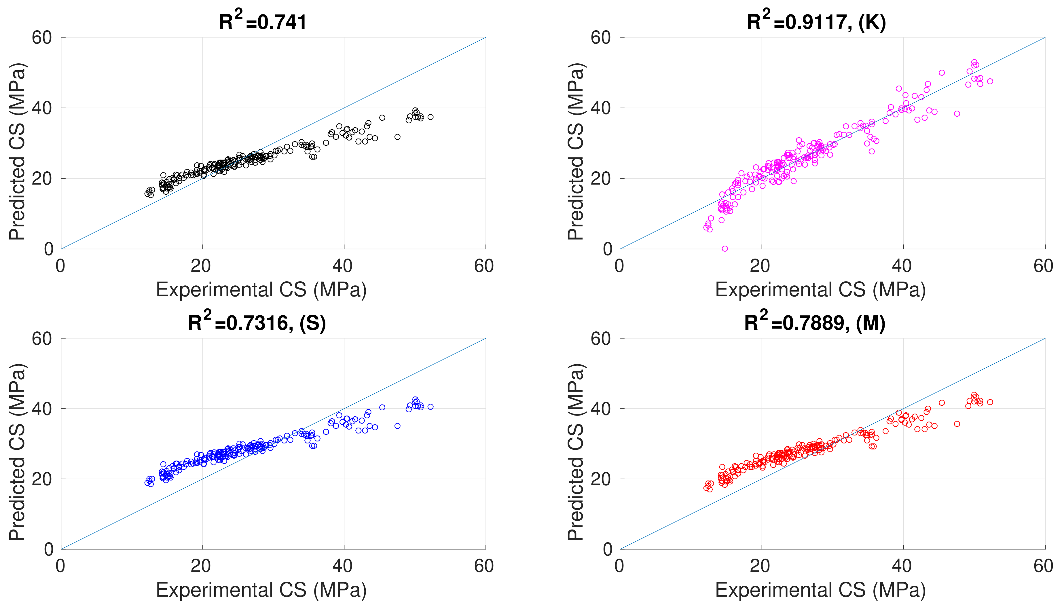Figure 1, Figure 2, Figure 3, Figure 4, Figure 5, Figure 6, Figure 7, Figure 8, Figure 9, Figure 10, Figure 11, Figure 12 and Figure 13 show the plot of the experimental versus predicted $CS$ for all the conversion models listed in Table 1. All the figures relate to the case of four cores used to evaluate and train all the calibration methods considered. Each figure is organized as follows: The upper right corner shows the plot related to the uncalibrated model predictions. The top left of the figure shows the plot associated with the GPR-calibrated model predictions. At the bottom left and bottom right, the figure shows the plots related to the shifted-factor- and multiplying-factor-calibrated model predictions, respectively.

Finally, the corresponding value of the correlation coefficient $R^2$ is given for each case to which the figure refers. The results shown in Figure 1, Figure 2, Figure 3, Figure 4, Figure 5, Figure 6, Figure 7, Figure 8, Figure 9, Figure 10, Figure 11, Figure 12 and Figure 13 confirm all the considerations we made by analyzing the results reported in Table 2, Table 3, Table 4 and Table 5, i.e., the GPR calibration procedure we propose allows all the conversion models we considered to improve the quality of the predicted CS values. This improvement can be easily deduced by observing how the data are located close to the line of best fit, i.e., the predicted $CS$ values better fit the experimental ones.

In summary, taking into account that each error metric provides a different lens under which to evaluate the performance of the models considered [42,43], the fact that all the metrics referring to the GPR calibration are, regardless of the number of samples considered, simultaneously better in the majority of cases compared to those offered by standard calibration techniques for the same number of samples confirms its effectiveness in providing a more precise and accurate calibrated conversion model compared to the conversion models calibrated in the standard way [44]. This result is undoubtedly due to the fact that the standard calibration methods provide constant calibration coefficients, one multiplicative and the other additive, which, once determined, are independent of the pair $[R_i,V_{p_i}]$ used as the input to the conversion model. In contrast, the GPR calibration technique provides a calibration that is a function of this pair, leading to better prediction results based on our numerical experiments, thanks to its ability to handle nonlinear relationships and uncertainties [25,28].

4. Conclusions

The calibration of SonReb conversion models available from previous studies is notably indicated in all cases where minimizing the number of DT measurements is essential. In this context, we propose a novel calibration approach based on GPR, taking advantage of its flexibility and inherent capability to quantify uncertainty over predictions. Its performance has been compared with traditional calibration procedures (shifting- and multiplying-factor calibration methods) using experimental data from the technical literature [29]. Once calibrated, the quality of the predictions offered by the SonReb conversion models is evaluated using the error metrics commonly used to rank regression models. Numerical results obtained with a small training dataset show that the GPR calibration is very effective, in most cases outperforming the standard techniques used to calibrate SonReb models with the same number of cores. However, even though the results provided by the GPR calibration approach are very promising, considering that Gaussian processes and kernel methods are closely related [27,45] and that kernels can offer a more viable way for nonparametric regression estimations [27], in future work, we will investigate the use of kernel methods for calibration, comparing and quantifying their performance against those offered by more standard machine learning methods, such as neural fuzzy networks [46] or support vector machines [47], also considering different and heterogeneous datasets taken from the literature and possibly from experimental SonReb measurements to further validate the generalizability of the results obtained in the present study.