Equivalent Morphology Concept in Composite Materials Using Machine Learning and Genetic Algorithm Coupling

Abstract

The objective of this study is to investigate the synergistic integration of machine learning and evolutionary algorithms for the discovery of equivalent morphologies exhibiting analogous behavior within the domain of composite materials. To pursue this objective, two comprehensive databases are meticulously constructed. The first database encompasses randomly positioned inclusions characterized by varying volume fractions and contrast levels. Conversely, the second database comprises microstructures of diverse shapes, such as elliptical, square, and triangular, while maintaining consistent volume fraction and contrast values across samples. Label assignment for both databases is conducted using a finite-element-method-based computational tool, ensuring a standardized approach. Machine learning techniques are then applied, employing distinct methodologies tailored to the complexity of each database. Specifically, an artificial neural network ANN model is deployed for the first database due to its intricate parameter configurations, while an eXtreme Gradient Boosting XGBoost model is employed for the second database. Subsequently, these developed models are seamlessly integrated with a genetic algorithm, which operates to identify equivalent morphologies with nuanced variations in geometry, volume fraction, and contrast. In summation, the findings of this investigation exhibit notable levels of adaptation within the discovered equivalent morphologies, underscoring the efficacy of the integrated machine learning and evolutionary algorithm framework in facilitating the optimization of composite material design for desired behavioral outcomes.

1. Introduction

Composite materials [1,2,3,4,5] represent a growing area of interest in engineering and materials science. Their ability to combine different properties from constituent materials makes them particularly attractive for a diverse range of applications, spanning from aerospace to automotive industries and construction. However, the optimal design of these materials remains a major challenge, especially when it comes to finding alternative morphologies that exhibit similar properties as existing materials.

In this regard, the use of bioinspired methods [6] such as machine learning [7,8] and evolutionary algorithms—notably, genetic algorithms—is emerging as a promising approach. These methods draw inspiration from biological processes and natural evolution to solve complex problems and find optimal solutions. The coupling of machine learning [9] and evolutionary algorithms [10,11] holds significant promise for addressing the challenges associated with the design of composite materials. Machine learning techniques, with their ability to analyze vast amounts of data and identify intricate patterns, offer valuable insights into the relationships between material properties, fabrication processes, and performance characteristics. By leveraging machine learning, researchers can uncover hidden correlations and optimize material design parameters to achieve desired outcomes. On the other hand, evolutionary algorithms provide a powerful optimization framework for exploring the vast design space of composite materials. By mimicking the process of natural selection, genetic algorithms can efficiently search for optimal material configurations that meet specified criteria, such as mechanical strength, thermal conductivity, or weight reduction. Through iterative generations and selection mechanisms, evolutionary algorithms iteratively refine and improve candidate designs and converge towards high-performing solutions.

When combined, machine learning and evolutionary algorithms create a synergistic framework for the discovery and optimization of composite material morphologies. Machine learning algorithms can be employed to analyze experimental data, identify promising design directions, and generate informative features for evolutionary optimization. In turn, evolutionary algorithms can leverage machine learning predictions to guide the search towards regions of the design space that are more likely to yield desirable outcomes.

Maridass et al. [12] employed a genetic algorithm and artificial neural networks to analyze blends comprising polypropylene and waste ground rubber tire powder. Their study focused on understanding how varying levels of ethylene–propylene–diene monomer EPDM and polypropylene grafted maleic anhydride PP-g-MA influence mechanical characteristics. By optimizing formulations to maximize tensile strength and contrasting them with blends optimized for maximum elongation at the breaking point, they observed that increased concentrations of PP-g-MA and EPDM enhanced properties: a finding corroborated through SEM investigations. Additionally, they established a quantitative correlation between polymer content and mechanical attributes. Azhar et al. [13] used the same coupling model to optimize the turning of glass-fiber-reinforced polymer GFRP composites. They aimed to find the best cutting parameters for efficient machining. By studying spindle speed, feed rate, and depth of cut effects on the material removal rate MRR, tool wear rate TWR, and surface roughness, they identified significant parameters and interactions. Empirical models linked output responses and cutting parameters, while ANN with GA achieved multi-response optimization. Santano et al. [14] integrated ANNs and GAs to study how stir-cast Al-Zn-Mg-Cu matrix composites behave under two-body abrasion. They examined the wear rate, coefficient of friction, and roughness of abraded surface RAS across various input parameters. Multi-objective optimization via Pareto solutions was utilized and highlighted the importance of particle quantity and abrasive size. Experimentation validates these findings, while analysis of micromechanisms and surface attributes clarifies their roles. The optimal condition for minimizing the wear rate and coefficient of friction while maintaining moderate RAS was determined to be 15 ± 2 wt% particle quantity. The same method was used by Zhen-jie et al. [15] to forecast the electromagnetic characteristics of coatings. Traditional methods face challenges in this regard due to the complexity of the parameters involved. Their approach effectively predicted EM properties, even when dealing with mixed absorbents, surpassing conventional ANN techniques. Furthermore, they employed GA to optimize coatings, resulting in enhanced electromagnetic absorption capabilities. Aveen et al. [16] used GA and ANN to improve drilling in composite materials. They investigated factors affecting hole quality in glass-fiber-reinforced composites by varying filler volumes (0%, 3%, and 6%) and drilling parameters. Data from drilling experiments were analyzed using Python-based neural networks, with GA optimizing conditions to reduce delamination. These method are not only valid for composite materials, but they can also be used for bio-composites. Madani et al. [17] employed an ANN-GA model to investigate surface roughness during milling of alfa/epoxy biocomposites, spanning both composite and bio-composite materials. Through 100 trials, they assessed the surface quality and the influence of the cutting parameters and chemical treatment. Their hybrid approach, merging ANN and GA, refined a predictive model for surface roughness and demonstrated enhanced accuracy compared to conventional methods. This findings underscored the importance of feed per revolution and chemical treatment in affecting surface roughness. Also, deeper in the nanocomposite field, Chi-Hua et al. [18] fused GA with deep learning DL to enhance nanocomposite toughness. Their AutoComp Designer algorithm merges machine learning and AI-improved genetic algorithms to enable the creation of new material designs with decreased computational expense. Through neural network training on diverse material combinations, they predicted the properties of graphene nanocomposites without conventional simulations. This technique not only forecasts properties but also enhances fracture toughness by adjusting the material distribution. Validation via molecular dynamics simulations verified the improved performance. In addition to ANNs, Adaboost has also been coupled to genetic algorithms: for example, by Weidong et al. [19] in order to optimize nanocomposite adsorption capacity. This approach aimed to streamline experiments and reduce costs by developing predictive models. They correlated adsorption parameters with capacity and used simple models due to having a small dataset. AdaBoost and GA optimization improved modeling efficiency. Data from the literature were utilized, resulting in highly efficient models with low error rates.

Our research aims to utilize ML-GA coupling to address the issue of equivalent morphology, which is a concept explored by Elmoumen et al. [20]. They compared two morphologies: one featuring overlapping identical spherical inclusions and the other with identical hard inclusions. Using numerical simulations and statistical analysis, they evaluate the representativeness of these structures. Their findings revealed a disparity in the integral range: while microstructures with hard spheres have an integral range equivalent to one inclusion’s volume, those with overlapping spheres exhibit an integral range eight times larger. This observation prompted the introduction of the equivalent morphology concept EMC. The EMC was also utilized by Khdir et al. [21,22] to develop a computational homogenization approach for porous media.

In this paper, we develop an innovative methodology to identify equivalent morphologies within a microstructure containing a circular inclusion using a coupling model based on the predictions of machine learning algorithms and the optimization of genetic algorithms. Our goal is to find alternative microstructures with different shapes, volume fractions, and phase contrasts that exhibit the same linear elastic and thermal behavior as the original microstructure. We employ advanced computational techniques to thoroughly analyze the microstructure’s linear elastic and thermal properties. At the core of our methodology is a model that integrates various machine learning algorithms, including artificial neural networks [23] and a highly effective gradient boosting framework [24] that is known for its performance with structured data. These algorithms significantly improve the predictive accuracy and efficiency of our analysis. To optimize the model’s parameters and accurately identify equivalent morphologies, we use a genetic algorithm. This algorithm, inspired by natural selection, iteratively refines a population of solutions to converge on an optimal set.

Section 1 focuses on acquiring diverse microstructures with varying shapes, volume fractions $V_f$, and contrast values C to compile a comprehensive database. Finite element simulations are used to determine mechanical properties. In Section 2, the dataset is split into two subsets. The first subset, with fixed $V_f$ and C values, feeds into an XGBoost model for each inclusion shape. The second subset, comprising circular microstructures with varying $V_f$ and C values, trains an artificial neural network model with integrated dropout layers. In the final section, by leveraging input parameters, the algorithms generate morphologies with equivalent mechanical properties but differing geometries. Additionally, circular microstructures with varied $V_f$ and C values are synthesized.

2. Data Collection Process

The profound complexity of the human brain offers compelling insights for enhancing machine learning models, including ANNs and XGBoost, owing to its unparalleled ability to learn from extensive datasets via observation, analysis, and iterative refinement. In simulating this cognitive paradigm, the efficacy of those models is intricately tied to the scale and diversity of the training data, wherein larger and more diverse datasets contribute to greater alignment between predicted and actual outcomes.

Our model’s input configuration integrates the spatial coordinates (x, y), the orientation angle $\theta$ relevant to elliptical with three different values of aspect ratios (1/3, 1/2, 2/3), square and triangular inclusions, the volume fraction $V_f$, and the phase contrast C. The contrast quantifies the level of heterogeneity within a heterogeneous material. When the value of C is significantly high (C >> 1) or extremely low (C << 1), it indicates a material with pronounced heterogeneity. Conversely, when C = 1, the material achieves complete homogeneity. In terms of elastic properties, the contrast is defined as the ratio between the Young’s modulus of the inclusion and that of the matrix (C = ${\displaystyle \frac{E_i}{E_m}}$). In contrast, for thermal properties, this ratio is determined by the thermal conductivity of both phases (C = ${\displaystyle \frac{{\lambda }_i}{{\lambda }_m}}$). These meticulously selected parameters are tailored for each 2D microstructure and serve as indispensable descriptors for a thorough characterization of the microstructural geometric attributes. Conversely, the output framework of our model encompasses distinct material properties, such as the bulk modulus, shear modulus, and thermal conductivity. These parameters serve as fundamental metrics for assessing the mechanical and thermal properties inherent to composite materials.

2.1. Microstructure Generation

2.1.1. Multi-Shape 2D Microstructure Generation

To address the primary optimization challenge, we divide the first dataset into four discrete sub-databases, each delineated by a distinct geometric entity: namely, circle, ellipse, square, and triangle, as shown in Figure 1. Within each sub-database, datasets are structured to encompass spatial coordinates (x and y) alongside inclusion orientation $\theta$ data. Moreover, consistent values are set for the volume fraction and phase contrast parameters to ensure uniformity throughout the analyses, with various scenarios tested involving volume fractions ranging from 10% to 30% and contrasts from 10 to 200. Through this iterative process, we aim to elucidate their nuanced effects on system performance. This rigorous approach not only seeks to optimize system efficiency but also aims to validate its reliability across the full range of input values. By conducting this exhaustive analysis, we anticipate uncovering optimal configurations across various scenarios, thereby enhancing our ability to effectively address the optimization challenge at hand.

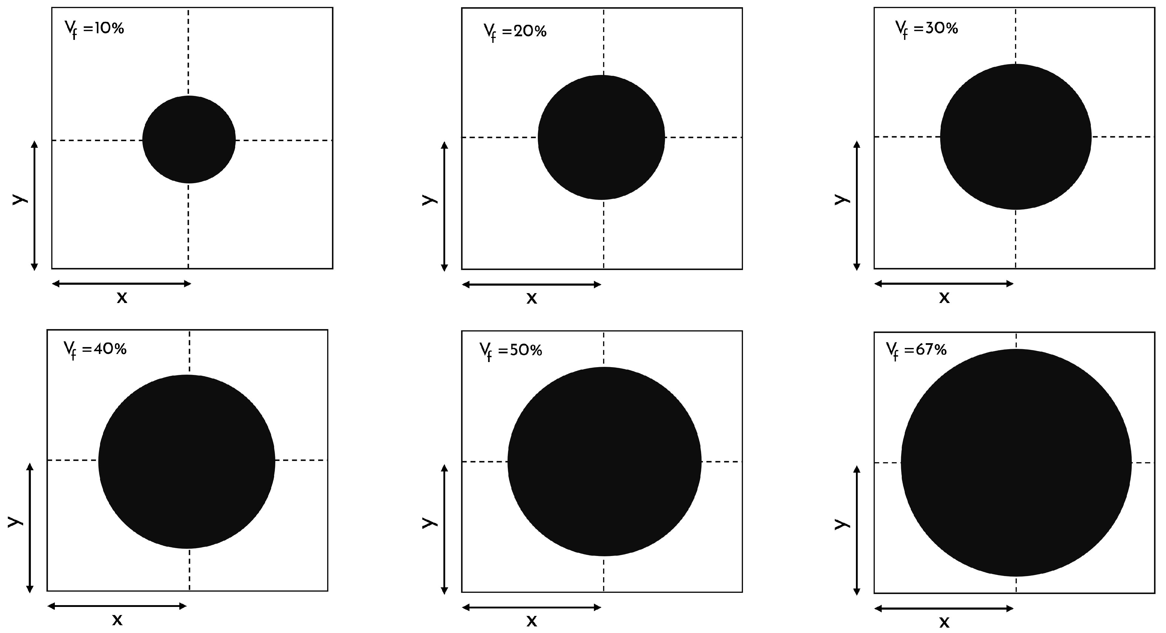
2.1.2. Circular 2D Microstructure Generation

The second database constitutes a pivotal stage within our analytical and optimization framework. Diverging from its predecessor, it incorporates more nuanced variable parameters tailored to exhaustively probe system performance. These parameters encompass four fundamental input variables: the abscissa (x), the ordinate (y), the volume fraction spanning from 10% to 67%, and, concurrently, the contrast between the two phases ranging from 10 to 200. It is imperative to note that the inclusion shapes consistently maintain circularity. Moreover, to ascertain the generation of random x and y values, we confine them within a specified interval predicated on the volume fraction, as shown in Figure 2. This methodological approach ensures the preservation of generated points within the confines of the predefined matrix.

2.2. Finite Element Calculations

The subsequent phase in our experimental process involves the acquisition of output data, which we term “Labels” within our model. These labels serve as the repository for the computed parameters and encompass critical metrics such as bulk, shear, and thermal conductivity. It is worth noting that this rigorous data acquisition process remains consistent across both databases, ensuring uniformity and reliability in our analyses. Our pursuit of understanding the effective elastic and thermal attributes of composite materials leads us to employ numerical homogenization, which is a cornerstone technique in numerical analysis. This method allows us to unravel the complex interplay of material properties within the composite structure. Leveraging the finite element (FE) method, we embark on a detailed examination of composite material behavior. This entails subjecting a square matrix reinforced with a singular circular, elliptical, square, or triangular inclusion to meticulous simulation and scrutiny.

While the matrix component of the composite exhibits consistent linear elastic and thermal behavior, characterized by predetermined values for Young’s modulus, Poisson’s ratio, and thermal conductivity, the behavior of the reinforcing inclusions varies markedly. This variability is contingent upon the chosen contrast value, which delineates the ratio of material properties between the inclusion and the matrix. In our numerical framework, the contrast value ranges from 10 to 200, representing a wide spectrum of material property disparities. Notably, we define the contrast value, denoted as C, as the ratio of the Young’s modulus and thermal conductivity between the inclusion and the matrix ($C={\displaystyle \frac{E_i}{E_m}}={\displaystyle \frac{{\lambda }_i}{{\lambda }_m}}$). Here, $E_i$ and ${\lambda }_i$ represent the Young’s modulus and thermal conductivity of the reinforcing inclusion, respectively, while $E_m$ and ${\lambda }_m$ signify those of the matrix phase.

The evaluation of the bulk modulus k and shear modulus $\mu$ involves formulas that incorporate the Young’s modulus E and Poisson’s ratio $\nu$ as follows:

$$\mu ={\displaystyle \frac{E}{2(1+v)}}\mathrm{and}k={\displaystyle \frac{E}{3(1-2v)}}$$

(1)

To ensure the accurate performance of finite element FE simulations, it is imperative to construct a mesh that faithfully captures the geometric intricacies of the analyzed system. In this particular investigation, we opted for a multi-phase element mesh configuration comprised of two-dimensional quadrilateral elements. This meshing strategy, depicted in Figure 3, was chosen to facilitate the simulation process and to enhance the reliability and fidelity of the results obtained from the FE analysis.

Boundary Conditions

In finite element analyses, boundary conditions [25,26] are of paramount importance. These conditions define the behaviors that a system must adhere to at its spatial or temporal boundaries. They enable the representation of external constraints and boundary traits, which, in turn, facilitates the attainment of accurate and reliable solutions for the system’s equations. By incorporating these conditions, we attain a holistic comprehension and predictive capability regarding the system’s overall behavior that encompasses external influences and interactions with the environment. To compute effective properties, we choose the same boundary conditions used in our previous papers [27,28].

Linear elasticity:

In this work, periodic boundary conditions to be prescribed on individual volume element V are considered:

The displacement field over the entire volume V takes the form:

$$\underline{u}=\underset{\sim }{E}·\underline{x}+\underline{v}\forall \underline{x}\in V,$$

(2)

where the fluctuation $\underline{v}$ is periodic. It takes the same values at two homologous points on opposite faces of V. The traction vector $\underset{\sim }{\sigma }·\underline{n}$ takes opposite values at two homologous points on opposite faces of V.

In our case, the periodic boundary conditions are considered as special cases for which specific values of $\underset{\sim }{E}$ and $\underset{\sim }{\sigma }$ are chosen. To compute effective properties in the case of periodic conditions, we choose an elementary volume with imposed macroscopic strain tensors as:

$$\underset{\sim }{E_k}=\left(\begin{array}{ccc}1& 0& 0\\ 0& 1& 0\\ 0& 0& 0\end{array}\right),\underset{\sim }{E_{\mu }}=\left(\begin{array}{ccc}0& {\displaystyle \frac{1}{2}}& 0\\ {\displaystyle \frac{1}{2}}& 0& 0\\ 0& 0& 0\end{array}\right)$$

(3)

An apparent bulk modulus $k^{\mathrm{app}}$ and an apparent shear modulus${\mu }^{\mathrm{app}}$ can be defined as:

$$\begin{array}{ccc}\hfill & k^{\mathrm{app}}={\displaystyle \frac{1}{2}}trace\langle \underset{\sim }{\sigma }\rangle \mathrm{and}\hfill & \hfill {\mu }^{\mathrm{app}}=〈{\sigma }_{12}〉\end{array}$$

(4)

where: $\underset{\sim }{\sigma }$ is the local stress tensor, ${\sigma }_{12}$ is the local shear tensor, and < > represents the average over the hole’s microstructure.

Thermal conductivity:

For the thermal problem, the temperature, its gradient, and the heat flux vector are denoted by $T,\nabla T$, and q, respectively. The heat flux vector and the temperature gradient are related by Fourier’s law, which reads:

$$\underline{q}=-\lambda \underline{\nabla T}$$

(5)

in the isotropic case. The scalar $\lambda$ is the thermal conductivity coefficient of the considered phase. A volume V of a heterogeneous material is considered again. For the linear elastic case, periodic boundary conditions are used in the study of the effective thermal conductivity:

The temperature field takes the form:

$$T=\underline{G}·\underline{x}+t\forall \underline{x}\in V$$

(6)

where t is periodic. Apparent conductivities coincide with the wanted effective properties for sufficiently large volumes V. To compute the effective thermal conductivity, the following test temperature gradient G and flux Q are prescribed on the elementary volume as:

$$\underline{G}=\left(\begin{array}{c}1\\ 1\\ 0\end{array}\right) \mathrm{and} \underline{Q}=\left(\begin{array}{c}1\\ 1\\ 0\end{array}\right)$$

(7)

They are used, respectively, to define the following apparent conductivities:

$${\lambda }^{\mathrm{app}}={\displaystyle \frac{1}{2}}trace\langle \underline{q}\rangle \mathrm{and}{\lambda }^{\mathrm{app}}={\displaystyle \frac{1}{2}}trace\langle \nabla \underline{T}\rangle$$

(8)

The periodic method was chosen for implementing the linear elasticity and thermal conductivity calculations due to its efficiency in terms of computation time while maintaining results comparable to alternative methods. Not only is this method the fastest, but it also offers a precise means of calculating the elastic properties of complex materials. Moreover, its relatively straightforward implementation makes it applicable to a diverse array of materials and geometries.

As previously mentioned, the heterogeneous material under study consists of a matrix embedded with a singular inclusion. The volume fraction’s value is adjusted during the microstructure generation phase, while the contrast value necessitates modification to the calculation files prior to initiating simulations. This involves altering the Young’s modulus and thermal conductivity values to align with specific research requirements.

For conducting finite element calculations with the designated software, several files are imperative: a matrix file detailing the first phase’s properties, an inclusion file for the second phase’s properties, a mesh file, and input files. Specifically, our study utilizes three input files tailored to assess the bulk properties, shear properties, and thermal conductivity. These files collectively enable the accurate modeling of the material’s response under varied testing scenarios.

3. Machine Learning Models

3.1. Data Pre-Processing and Splitting

Prior to constructing neural networks, it is essential to undergo data preprocessing, which is a critical stage involving the normalization of input features such as the abscissa, ordinate, and inclusion orientation. Normalization plays a pivotal role in standardizing these feature values, thereby ensuring efficient and effective model convergence. This process is facilitated through the utilization of the StandardScaler() function, which is indispensable for adjusting the data by subtracting the mean $\mu$ and dividing by the standard deviation $\sigma$. Mathematically, this normalization technique is represented by the equation:

$$X_{\mathrm{normalized}} ={\displaystyle \frac{X-\mu }{\sigma }}$$

(9)

Here, X represents the input data, $\mu$ denotes the mean, and $\sigma$ signifies the standard deviation. By applying this normalization technique, all input features contribute equally to the neural network’s learning process, thereby promoting stability and enhancing performance throughout the training phase.

Furthermore, it is customary to divide the dataset into three distinct subsets: the training set, the validation set, and the test set. Each subset serves a unique purpose in the model development process. The training set is utilized to train the model’s parameters, enabling it to discern patterns and relationships within the data. The validation set assumes a crucial role in fine-tuning hyperparameters and assessing the model’s performance during training. Finally, the test set remains reserved for evaluating the model’s ability to generalize to unseen data, providing a reliable measure of its performance post-training and validation.

In our approach, we allocate 80% of the dataset for training, which includes the validation subset, while reserving the remaining 20% for testing. This partitioning strategy ensures an ample amount of data for model training and validation while also maintaining a separate portion for assessing the model’s performance on unseen data. Such meticulous partitioning is vital for ensuring the robustness and reliability of the trained model.

3.2. Prediction of the Thermomechanical Behavior of 2D Circular Microstructure with Various Volume Fraction and Contrast Values

3.2.1. Model Architecture

This intricately designed neural network architecture, which is constructed using Keras’s Sequential API, meticulously orchestrates a series of interconnected layers to proficiently process input data. At its core lies a dense layer housing 128 neurons, which are strategically selected for their ability to discern intricate patterns within the input dataset. By harnessing the ReLU activation function, this layer introduces crucial non-linearity, enhancing the model’s capacity to capture complex relationships.

Subsequently, a dropout layer is seamlessly incorporated, with the dropout rate set to 0.2. This regularization technique combats overfitting by selectively deactivating 20% of the neurons during training, fostering robust generalization. The deliberate inclusion of dropout layers at strategic junctures in the network underscores a meticulous effort to balance model intricacy with regularization. Continuing the network’s progression, another dense layer emerges, featuring 64 neurons and embracing the ReLU activation function. Like its precursor, this layer perpetuates the propagation of non-linear transformations throughout the network, enabling the extraction of intricate features from the input data. The subsequent dropout layer, matching its predecessor with a dropout rate of 0.2, fortifies the model against overfitting, thereby bolstering its capacity for resilient generalization. This methodical integration of dropout layers underscores a proactive approach to regularization, ensuring the model’s adeptness at capturing essential patterns while mitigating the risk of memorizing noise.

As the network unfolds, a third dense layer materializes, housing 64 neurons and employing the ReLU activation function. This layer serves as an additional conduit for non-linear transformations, facilitating the extraction of increasingly complex features from the input data.

Finally, the output layer takes form as a dense layer housing a single neuron, representing the model’s ultimate objective of direct linear regression. In this configuration, no activation function is specified, signifying a straightforward mapping of input features to output predictions. Figure 4 below explains the detailed architecture of the ANN model.

3.2.2. Model Compilation

The compilation of a model stands as the final stage in its creation and is crucial for predicting optimal optimization decisions. This process involves setting three key parameters: the optimizer, loss function, and metrics.

The optimizer dictates the learning rate, influencing the speed at which the model computes optimal weights. In our case, “Adam” serves as our optimizer and dynamically adjusts the learning rate during training. Adam integrates two gradient descent methodologies:

Momentum: Momentum is utilized to expedite the gradient descent process by incorporating an exponentially weighted average of gradients. This accelerates convergence towards the minimal value. The update rule involves the current weight being adjusted by subtracting the product of the learning rate and the momentum.

$$w_{t+1}=w_t-\alpha m_t$$

(10)

where:

-

$w_t$ represents the weights at time t;

-

$m_t$ denotes the aggregate of gradients at time t;

-

$\alpha$ signifies the learning rate;

-

${\displaystyle \frac{\delta L}{\delta w_t}}$ is the derivative of the loss function with respect to the weights at time t;

-

$\beta$ is the moving average parameter (typically 0.9).

Root mean square propagation RMSP: RMSP is an adaptive learning algorithm that improves upon AdaGrad. Unlike AdaGrad, which accumulates squared gradients, RMSP computes an exponential moving average.

$$w_{t+1}=w_t-{\displaystyle \frac{{\alpha }_t}{{\left(v_t+\epsilon \right)}^{1/2}}}\left[{\displaystyle \frac{\delta L}{\delta w_t}}\right]$$

(11)

where:

-

$w_t$ represents the weights at time t;

-

$v_t$ is the sum of the squares of past gradients;

-

${\alpha }_t$ signifies the learning rate at time t;

-

${\displaystyle \frac{\delta L}{\delta w_t}}$ is the derivative of the loss function with respect to the weights at time t;

-

$\beta$ is the moving average parameter (typically 0.9);

-

$\epsilon$ is a small positive constant (usually ${10}^{-8}$).

Loss function: The loss function serves to measure the discrepancy between the predicted and actual values during the learning phase. In constructing our model, we opt for the mean absolute percentage error MAPE, which is a widely adopted metric for regression tasks. A lower MAPE value indicates better model performance, as it signifies a smaller deviation between predicted and true values. Its formula is expressed as:

$$\mathrm{MAPE}={\displaystyle \frac{1}{n}}\sum _{i=1}^n\left|{\displaystyle \frac{T_i-P_i}{T_i}}\right|$$

(12)

where:

-

n is the number of fitted points;

-

$T_i$ is the actual value;

-

$P_i$ is the predicted value.

Metrics: The metrics serve as the criteria for assessing the model’s performance, akin to the loss function, albeit they are not utilized during training. Within our model, we select the mean absolute error (MAE) as our metric of choice. MAE quantifies the accuracy of the model by evaluating the average absolute difference between predicted and actual values.

$$\mathrm{MAE}={\displaystyle \frac{1}{n}}\sum _{j=1}^n\left|T_j-P_j\right|$$

(13)

where:

-

n is the number of fitted points;

-

$T_j$ is the actual value;

-

$P_j$ is the predicted value.

3.2.3. Training and Evaluation

Figure 5 visually presents the loss function, which is a pivotal measure utilized to assess our model’s performance. This function serves to quantify the disparity between the model’s predicted values and the actual data values within the dataset. By tracking the behavior of the loss function throughout the training process, we gain valuable insights into the model’s learning dynamics and its ability to adapt to the dataset.

The blue curve delineates the trajectory of the training data’s error rate as the model progresses through successive epochs of training. Initially, this error rate is notably high, reflecting substantial disparities between the model’s initial predictions and the actual target values. This disparity primarily stems from the random initialization of weights at the onset of training. However, as the model iteratively learns from the training data and adjusts its parameters, the error rate gradually diminishes, signifying an enhancement in the model’s predictive accuracy. This gradual reduction continues until the error rate converges towards its minimum value, indicating the model’s proficiency in capturing the underlying data patterns. Conversely, the red curve depicts the prediction error observed on the validation dataset, which comprises data that the model did not encounter during training. Mirroring the trend observed in the training curve, the validation error also exhibits a decreasing trajectory over epochs, suggesting the model’s capacity to generalize effectively to unseen data instances. The convergence of the validation error towards the minimum value observed in the training curve reinforces the model’s capability to make precise predictions across various datasets.

Upon reaching convergence, the error function stabilizes within a narrow range: typically equal to 75 epochs. This stability signifies that the model has attained a consistent level of accuracy in predicting the target variables, underscoring its reliability and efficacy.

The final phase is prediction, which represents the culmination of our model generation process and marks the critical moment when the anticipated outcomes of our model are realized. It involves applying the prediction model to the test dataset, followed by an intricate comparative analysis between the resulting predictions and the actual values of the shear, bulk, and thermal moduli. This meticulous examination serves as the foundation for computing the coefficient of determination $R^2$, which is a fundamental metric for evaluating the model’s predictive power.

$$R^2=1-{\displaystyle \frac{{\sum }_{i=1}^n{\left(y_i-{\widehat{y}}_i\right)}^2}{{\sum }_{i=1}^n{\left(y_i-\overline{y}\right)}^2}}$$

(14)

where:

$y_i$ is the actual value;

${\widehat{y}}_i$ is the predicted value.

Moreover, the $R^2$ metric, also known as the Pearson linear coefficient of determination, serves as a cornerstone in evaluating the efficacy of our linear regression predictions. Its value ranges from 0 to 1, with higher values indicating a stronger correlation between the predicted and actual values, reflecting the model’s predictive accuracy.

Upon subjecting our model to rigorous testing using the initial test images from the principle database, we achieved an impressive $R^2$ score of 0.98. This noteworthy result underscores the robustness and appropriateness of the chosen model parameters, affirming our confidence in its predictive capabilities. To enhance our understanding and interpretation of the prediction outcomes, we employ regression curves as visual aids. These curves offer a clear representation of the relationship between the predicted and actual values, facilitating a more intuitive comprehension of the underlying predictive patterns. By plotting the regression lines against the dataset’s actual values, we gain valuable insights into the model’s performance and its ability to accurately predict the target variables.

The accompanying Figure 6 and Figure 7 provide a comprehensive visualization of the prediction outcomes for various modulus values, including bulk, shear, and thermal conductivity. Notably, the close alignment of the majority of data points with the linear regression line suggests strong correspondence between the predicted and actual values. This observation further bolsters our confidence in the regression model’s ability to accurately capture the complex relationships inherent in the dataset, thereby validating its utility in other cases.

3.3. Prediction of the Thermomechanical Behavior of a Multishape 2D Microstructure with Fixed Volume Fraction and Contrast Values

3.3.1. Model Definition

The gradient boosting regressor (GBR) is an iterative ensemble learning technique used primarily for regression tasks. It operates by sequentially training a series of weak learners—typically, decision trees—to enhance the overall predictive performance. At each iteration, a new weak learner is trained to minimize the negative gradient of the loss function relative to the previous model’s predictions. This is aimed at reducing the overall loss. Mathematically, the prediction at iteration m for a given input $x_i$ is calculated as:

$${\widehat{y}}_i^{\left(m\right)}={\widehat{y}}_i^{(m-1)}+\nu ·{\mathrm{tree}}_m\left(x_i\right)$$

(15)

where ${\widehat{y}}_i^{\left(m\right)}$ represents the predicted value at iteration m, ${\widehat{y}}_i^{(m-1)}$ is the prediction from the previous iteration, $\nu$ denotes the learning rate, and ${\mathrm{tree}}_m\left(x_i\right)$ signifies the prediction of the m-th decision tree for input $x_i$.

The GBR algorithm aims to minimize the loss function $L(y,\widehat{y})$ with respect to the predicted values $\widehat{y}$, where y signifies the true target values. The final prediction is derived by summing the predictions of all weak learners:

$${\widehat{y}}_i=\sum _{m=1}^M{\widehat{y}}_i^{\left(m\right)}$$

(16)

where M represents the total number of iterations.

The training process of the GBR algorithm involves initializing the model with a constant value and refining it iteratively. At each iteration, the algorithm computes the residuals, trains a regression tree to predict these residuals, computes optimal weights for each terminal node of the tree, and updates the model accordingly. This iterative process continues for M iterations, resulting in an ensemble model that minimizes the mean squared error loss function $L(y,\widehat{y})$. This enables the model to effectively capture complex relationships within the data and make accurate predictions.

Algorithm:

• Initialize model with a constant value:

  $$F_0\left(x\right)=\underset{\gamma }{argmin}\sum _{i=1}^{n}L\left(y_i,\gamma \right)$$
• For $m=1$ to M (number of iterations):

  (a)

  Compute residuals:

  $$r_{im}=-{\left[{\displaystyle \frac{\partial L\left(y_i,F\left(x_i\right)\right)}{\partial F\left(x_i\right)}}\right]}_{F\left(x\right)=F_{m-1}\left(x\right)}\mathrm{for}i=1,\dots ,n$$

  (b)

  Train regression tree: Train a regression tree with features x against residuals r and create terminal node regions $R_{jm}$ for $j=1,\dots ,J_m$

  (c)

  Compute optimal weights:

  $${\gamma }_{jm}=\underset{\gamma }{argmin}\sum _{x_i\in R_{jm}}L\left(y_i,F_{m-1}\left(x_i\right)+\gamma \right)\mathrm{for}j=1,\dots ,J_m$$

  (d)

  Update the model:

  $$F_m\left(x\right)=F_{m-1}\left(x\right)+\nu \sum _{j=1}^{J_m}{\gamma }_{jm}1\left(x\in R_{jm}\right)$$

where:

• $F_m\left(x\right)$ represents the prediction at iteration m for input x;
• $\nu$ is the learning rate;
• $L(y,F(x\left)\right)$ is the loss function measuring the discrepancy between the true target values y and the predicted values $F\left(x\right)$;
• $r_{im}$ are the residuals at iteration m;
• $R_{jm}$ are the terminal node regions of the regression tree at iteration m;
• ${\gamma }_{jm}$ are the optimal weights for each terminal node region at iteration m;
• $J_m$ is the number of terminal node regions in the regression tree at iteration m.

In our study, we meticulously optimized the GBR model to enhance its performance in predicting continuous values within our dataset. Utilizing the grid search technique, we systematically explored a broad spectrum of hyperparameter configurations. This involved a comprehensive examination of key hyperparameters, including the number of estimators (n_estimators), where we scrutinized values of 200, 300, 400, and 500, representing the number of boosting stages (trees) within the ensemble. Similarly, we carefully assessed various learning rates (learning_rate), including 0.05, 0.1, 0.15, and 0.2, to regulate the contribution of each tree to the overall ensemble. Moreover, depths spanning from 4 to 7 were considered for the maximum depth of trees (max_depth) to manage the complexity of individual trees within the ensemble. We also evaluated split thresholds of 3, 5, 7, and 10 samples for the minimum number of samples for splitting nodes (min_samples_split), significantly impacting the process of constructing trees. Additionally, our exploration encompassed the minimum number of samples required to form a leaf node (min_samples_leaf), with values ranging from 2 to 5. Furthermore, we meticulously examined subsampling rates (subsample) of 0.7, 0.8, 0.9, and 1.0 to introduce randomness and alleviate overfitting. Employing a rigorous five-fold cross-validation approach, we thoroughly assessed the model’s performance across an array of hyperparameter combinations, ensuring robustness and reliability in our evaluations. Following this exhaustive search, we pinpointed the optimal hyperparameter values that maximized performance metrics such as the R-squared score and minimized the mean squared error. Armed with these optimal configurations, we proceeded to train a new GBR model on the complete training dataset. Subsequently, we meticulously evaluated the performance of this tuned model on an independent test dataset, thereby gauging its predictive accuracy and generalization capability. Through this meticulous optimization process, we successfully crafted a highly effective and dependable predictive model tailored to the unique characteristics of our dataset.

3.3.2. Model Compilation

The process of compiling and training the model closely resembles that of the previously employed ANN, with one significant departure: the substitution of the the mean squared error MSE loss function for MAPE. This preference for MSE in XGBoost models addressing regression issues stems from its unbiased treatment of positive and negative errors as well as its differentiability, which facilitates the optimization of the gradient boosting algorithm. The MSE is computed using the formula:

$$\mathrm{MSE}={\displaystyle \frac{1}{n}}\sum _{i=1}^n{(Y_i-{\widehat{Y}}_i)}^2$$

(17)

where $Y_i$ represents the actual values, ${\widehat{Y}}_i$ denotes the predicted values, and n refers to the total sample count.

3.3.3. Training and Evaluation

Figure 8 offers a nuanced analysis of the fluctuation in training and validation error across six distinct geometric forms, contingent upon the sample size employed during the learning process. This graphical representation serves to elucidate the manner in which model efficacy varies in relation to dataset magnitude. A primary observation centers on the rapid convergence of curves toward values proximal to zero for each geometric configuration. This convergence intimates the models’ adeptness in assimilating information from the available data. As the sample size expands, both training and validation errors exhibit a gradual decline, indicative of the models’ adept adaptation to data intricacies and their proficient extrapolation across heterogeneous data landscapes.

Moreover, upon scrutinizing the MSE values, a discernible correlation with the complexity of the geometric shapes emerges. The least intricate form, the circle, manifests the lowest MSE, owing to the model’s reliance on solely two input variables (x, y) for its characterization, thereby streamlining the learning process. Conversely, the apex of complexity, embodied by the triangle, evinces the highest MSE, primarily due to its more stringent constraints: particularly, the limitation of angles to less than 60 degrees. This augmented complexity renders the capture of data variability more arduous, consequently engendering heightened predictive errors. These observations underscore the paramount significance of accounting for data complexity in the development and selection of machine learning models. Shapes of greater complexity may necessitate more nuanced models or augmented dataset sizes to attain optimal performance. Conversely, shapes of lesser complexity may be effectively encapsulated by simpler models, fostering superior overall performance and diminished error margins.

Transitioning to the prediction phase, we utilized the coefficient of determination $R^2$ as our primary evaluation metric. Figure 9, Figure 10 and Figure 11 below present the prediction results of the bulk modulus through three different scenarios. Across our investigation encompassing three distinct scenarios, where we systematically adjusted contrast values and volumetric fractions, we uncovered compelling predictive capabilities. Notably, our assessments unveiled a consistent trend of high-quality predictions across various geometric shapes within each scenario.

Upon closer examination of the results, a noteworthy observation emerges: the test data points closely adhere to the $y=x$ line, indicating robust predictive accuracy. This alignment translates into impressive prediction scores ranging from 0.91 to 0.99 across the different scenarios. Notably, these scores fall within the performance spectrum observed between the triangular and circular shapes, echoing the complexities identified during model training.

The commendable predictive performances underscore the meticulous selection of hyperparameters within the XGBoost framework. Particularly, the adoption of the grid search methodology proved instrumental in identifying optimal parameter configurations, regardless of the dataset’s geometric complexity. This meticulous approach to hyperparameter tuning not only ensures robust generalization but also instills confidence in the model’s consistent and reliable performance across datasets exhibiting diverse geometric shapes.

4. Optimal Generation of Equivalent 2D Microstructure

4.1. Defining Desired Microstructure Behaviors

The primary objective of this study is to elucidate the equivalent morphology of a microstructure embedded within a composite material featuring a randomly positioned circular inclusion. This investigation rigorously considers the influence of fixed values of contrast and volumetric fraction on the material’s behavior across both the elastic and thermal domains.

The overarching aim is to leverage two distinct databases as shown in Figure 12 to accomplish the following dual-fold objectives:

• Determine an alternative morphology that mirrors the original microstructure’s essential characteristics in terms of volumetric fraction and contrast, albeit manifesting a different geometric configuration. This exploration encompasses geometric variations such as elliptical, square, or triangular shapes.
• Explore the possibility of identifying an alternative morphology with a comparable geometric shape to the original microstructure while manifesting distinct values of volumetric fraction and contrast.

Within this context, the optimization problem can be articulated in a detailed manner:

4.2. Objective Function Formulation

We designate $K_{\mathrm{pr}},{\mu }_{\mathrm{pr}},{\lambda }_{\mathrm{pr}}$ as the elastic and thermal moduli characterizing the base microstructure. Our objective is to determine the optimal position $(x,y)$, orientation $\theta$, and morphology of the inclusion, ensuring it emulates the behavior of the base microstructure. Additionally, we aim to precisely identify the inclusion’s spatial coordinates $(x,y)$, alongside quantifying the volume fraction and contrast between the two phases to accurately replicate this desired behavior.

The optimization task is geared towards maximizing the objective function within the confines of constraints dictated by the predetermined values of the elastic parameters K, $\mu$, and $\lambda$. This comprehensive optimization process must meticulously consider the intricate interplay of elastic and thermal properties all while maintaining strict adherence to the specified parameter values. Consider the optimization problems:

$$\left\{\begin{array}{c}\begin{array}{cc}& \mathbf{Find}\mathrm{the}\mathrm{best}\mathrm{set}(X,Y,V_f,C)\hfill \\ & \mathbf{subject}\mathbf{to}:\hfill \\ & 0<X,Y<1000\hfill \\ & 5\%<V_f<67\%,10<C<200\hfill \\ & \mathbf{leading}\mathbf{to}\mathrm{prescribed}\mathrm{values}:\hfill \\ & K=K_{\mathrm{pr}},\mu ={\mu }_{\mathrm{pr}},\lambda ={\lambda }_{\mathrm{pr}}\hfill \end{array}\hfill \end{array}\right.\left\{\begin{array}{c}\begin{array}{cc}& \mathbf{Find}\mathrm{the}\mathrm{best}\mathrm{set}(X,Y,\theta )\hfill \\ & \mathbf{subject}\mathbf{to}:\hfill \\ & X1,Y1<X,Y<X2,Y2,0<\theta <180\hfill \\ & \mathbf{leading}\mathbf{to}\mathrm{prescribed}\mathrm{values}:\hfill \\ & K=K_{\mathrm{pr}},\mu ={\mu }_{\mathrm{pr}},\lambda ={\lambda }_{\mathrm{pr}}\hfill \end{array}\hfill \end{array}\right.$$

where $K_{\mathrm{pr}},{\mu }_{\mathrm{pr}},{\lambda }_{\mathrm{pr}}$ represents the prescribed values.

To achieve the first goal, we maximize the fitness function $f\left(A\right)$, defined as:

$$f\left(A\right)={\displaystyle \frac{1}{\left|A-A_{pr}\right|+1}}$$

(18)

This function evaluates the proximity of the inclusion parameters A to the optimal state $A_{pr}$, where a higher value of $f\left(A\right)$ indicates a closer resemblance to the optimal behavior.

Simultaneously, our endeavor involves minimizing the discrepancy $\left|A-A_{pr}\right|$, which reflects the deviation of the inclusion parameters from their optimal values.

Through this optimization process, we aim to achieve both objectives effectively, aligning the inclusion properties with the desired performance criteria.

4.3. Genetic Algorithm

Initially, our goal is to tackle the challenge of achieving equivalent morphology using bioinspired methods, including genetic algorithms. The decision to employ genetic algorithms was driven by specific criteria relevant to our problem. GAs were chosen to determine composite morphology due to unique characteristics inherent to our research problem that other optimization methods struggle to handle effectively. The behavior of composites is influenced by multiple variables including the distribution, shape, orientation, and interaction of different material phases. These relationships are typically non-linear and involve complex interactions and synergistic effects that are challenging to model using conventional optimization techniques. Moreover, the response surface for the optimal morphology of a composite may feature numerous local optima. GAs, which directly manipulate real composite design parameters using specific genetic operators, are particularly adept at avoiding local optima and seeking the global optimum, which is a critical capability in our scenario, where straightforward solutions are insufficient. Genetic algorithms GAs are a subset of evolutionary algorithms EAs, which are widely recognized for their effectiveness in handling complex, multi-modal, and large-scale optimization problems. These stochastic search methods draw inspiration from the natural evolutionary process [29,30] and evolve a population of candidate solutions over successive generations. In this study, we delve into the genetic algorithm approach and utilize it to navigate through the optimization landscape of the problem at hand.

The foundational principle of GAs is rooted in the mechanisms of natural selection, where individuals within a population, each representing a potential solution characterized by an objective function or fitness, undergo evolutionary processes. The core idea is that the fittest individuals have a higher likelihood of being chosen to produce offspring for the next generation. This selection process is augmented by genetic operators that mimic biological evolution, including selection, crossover, and mutation [30,31]:

-

**Selection**: a stage that prioritizes individuals with higher fitness scores, granting them a greater chance to contribute their genetic material to the next generation.

-

**Crossover**: a recombination process that merges the genetic information of selected parents to generate offspring, thereby exploring new regions of the solution space.

-

**Mutation**: introduces random genetic variations to some offspring, preventing premature convergence to local optima and encouraging diversity within the population [32,33].

This simulated evolutionary cycle, marked by selection, reproduction, and mutation, is iterated over numerous generations. The GA’s objective is to identify the most optimal solution—i.e., the individual with the highest fitness—across all generations.

While traditional approaches often employ a binary representation for optimization parameters, our study adopts the direct manipulation of integer and real-number parameters, in alignment with contemporary practices. The optimization begins with the generation of an initial, random population, followed by the application of genetic operations, which were carefully selected based on precedents from the literature [30]. Key operations include tournament selection for choosing parents, whole arithmetical crossover for creating offspring, and random uniform mutation for introducing genetic diversity.

The GA process incorporates elitism to ensure the best solution from one generation is carried over to the next, thus preserving advantageous traits. Through iterations of these genetic operations, the GA progresses towards identifying the optimal solution.

The configuration of the genetic algorithm, including the specific genetic operators and their probabilities ($p_{cross}$ for crossover and $p_{mut}$ for mutation) as well as the selection strategy for the crossover point $\rho$, follows the guidelines and recommendations outlined in the literature [30,31]. These parameters are finely tuned based on empirical evidence and preliminary testing to optimize the algorithm’s performance for the specific challenges presented by the optimization problem.

In numerical experiments, the choice of population size and number of generations is carefully tailored to the complexity of the optimization problems at hand [32,33]. By selecting 300 individuals and conducting 2000 generations, we aim to strike a balance between computational efficiency and thorough exploration of the solution space. These values are carefully selected based on considerations aligned with the nature and intricacy of the optimization problems under investigation (Figure 13).

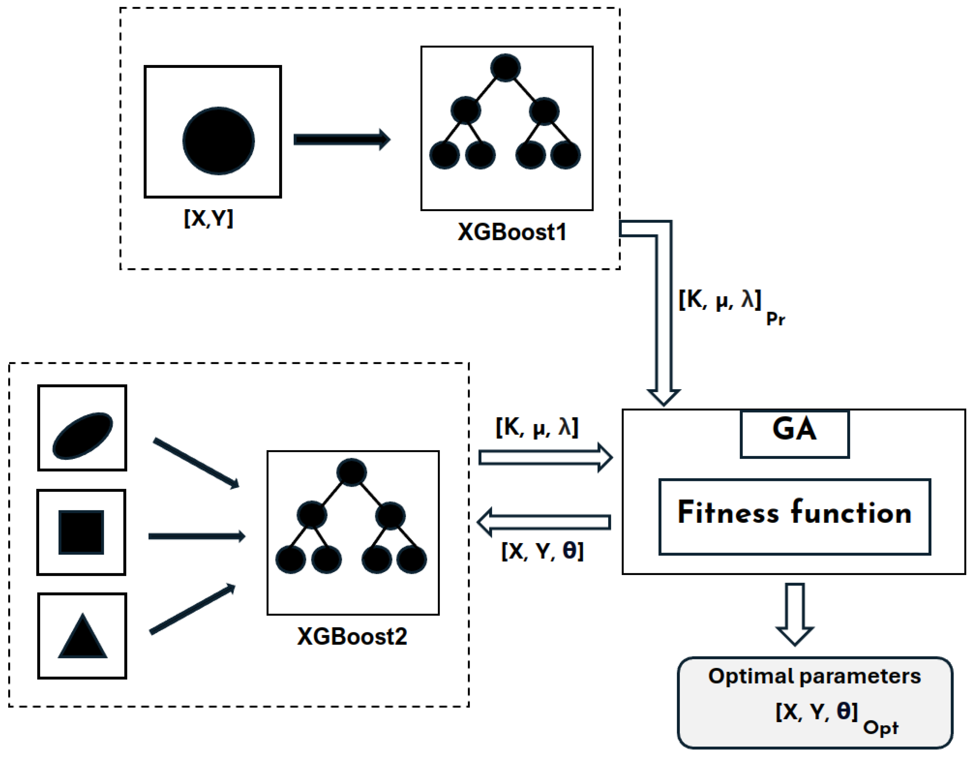
4.4. Search for Equivalent Morphology Using the Coupling of Machine Learning and the Genetic Algorithm

In order to solve the optimization challenge, an innovative approach has been devised to integrate two bioinspired methodologies seamlessly. In this novel strategy, the GA assumes a central role overseeing the evaluation of individuals’ fitness in each generation. Traditionally, fitness computation for analogous mechanical problems involves using simulation software like finite element methods, which can be time-intensive, especially with large datasets. To overcome this challenge, machine learning has been integrated into the GA framework. Unlike conventional methods, ML models pre-trained on fitness data are employed. These ML models exhibit remarkable accuracy, with prediction scores ranging from 0.92 to 0.99, thereby eliminating the need for resource-intensive simulations. During the GA execution, these ML-generated predictions seamlessly blend into the crossover and mutation processes. Consequently, this hybrid approach optimally leverages the synergies between GA and ML, resulting in a significant acceleration of the optimization process while ensuring precise and meticulous fitness evaluations.

4.4.1. Equivalent Over-Form Inclusion

To address the primary optimization challenge, we implement a genetic algorithm in conjunction with XGBoost models trained on diverse datasets featuring various shape configurations, as shown in Figure 14. The objective is to identify the optimal parameters x, y, and $\theta$ that maximize a specific fitness function while simultaneously minimizing the discrepancies between the predicted values for the circular shape $A_{pr}$ and those for other shapes. The genetic algorithm systematically explores different parameter combinations x, y, and $\theta$ by leveraging XGBoost models to predict properties associated with different shapes. Through iterative adjustments to these parameters, the algorithm aims to enhance the agreement between predicted and target values for the circular shape. Essentially, it seeks parameter configurations that yield predictions most closely resembling the properties of a circular shape. Upon completion of the optimization process, the genetic algorithm provides the most effective parameter combinations, resulting in the best fits for various shapes. These combinations represent parameters conducive to achieving property values closely aligned with those of the circular shape, thereby fulfilling the optimization objective.

4.4.2. Equivalent Circular Inclusions

Moving on to the second optimization challenge, we encounter a distinct scenario where only a single neural network model is utilized. Within this framework, the fitness function invokes an artificial neural network model that is specifically configured to accommodate randomly generated circular microstructures exhibiting diverse contrast values and volume fractions, as shown in Figure 15. The primary objective of the genetic algorithm in this context is to ascertain the optimal parameters (X, Y, $V_f$, and C) that minimize the discrepancy between the prescribed value and the output provided by the model. To mitigate the risk of the GA converging towards identical solutions across iterations, a sophisticated algorithm has been developed. This algorithm operates at each iteration and introduces a penalty to the fitness function equivalent to the value of the previous solution. By imposing this penalty, the algorithm encourages the model to explore alternative solutions, thereby enhancing the diversity of the parameter space explored. For comprehensive insights into the intricacies of this algorithm, readers are directed to consult the preceding paper, where the algorithm is meticulously elucidated. The coupling of the GA with the ANN model stands poised to yield optimal parameter configurations capable of maximizing fitness across a spectrum of microstructural variations. This nuanced approach endeavors to achieve behaviors closely aligned with the prescribed criteria while allowing for nuanced adjustments in parameters such as X, Y, $V_f$, and C. Through this methodical exploration of the parameter space, the GA effectively navigates the landscape of potential solutions, facilitating the identification of configurations that manifest the desired behavioral traits with precision and reliability.

4.4.3. Results and Discussions

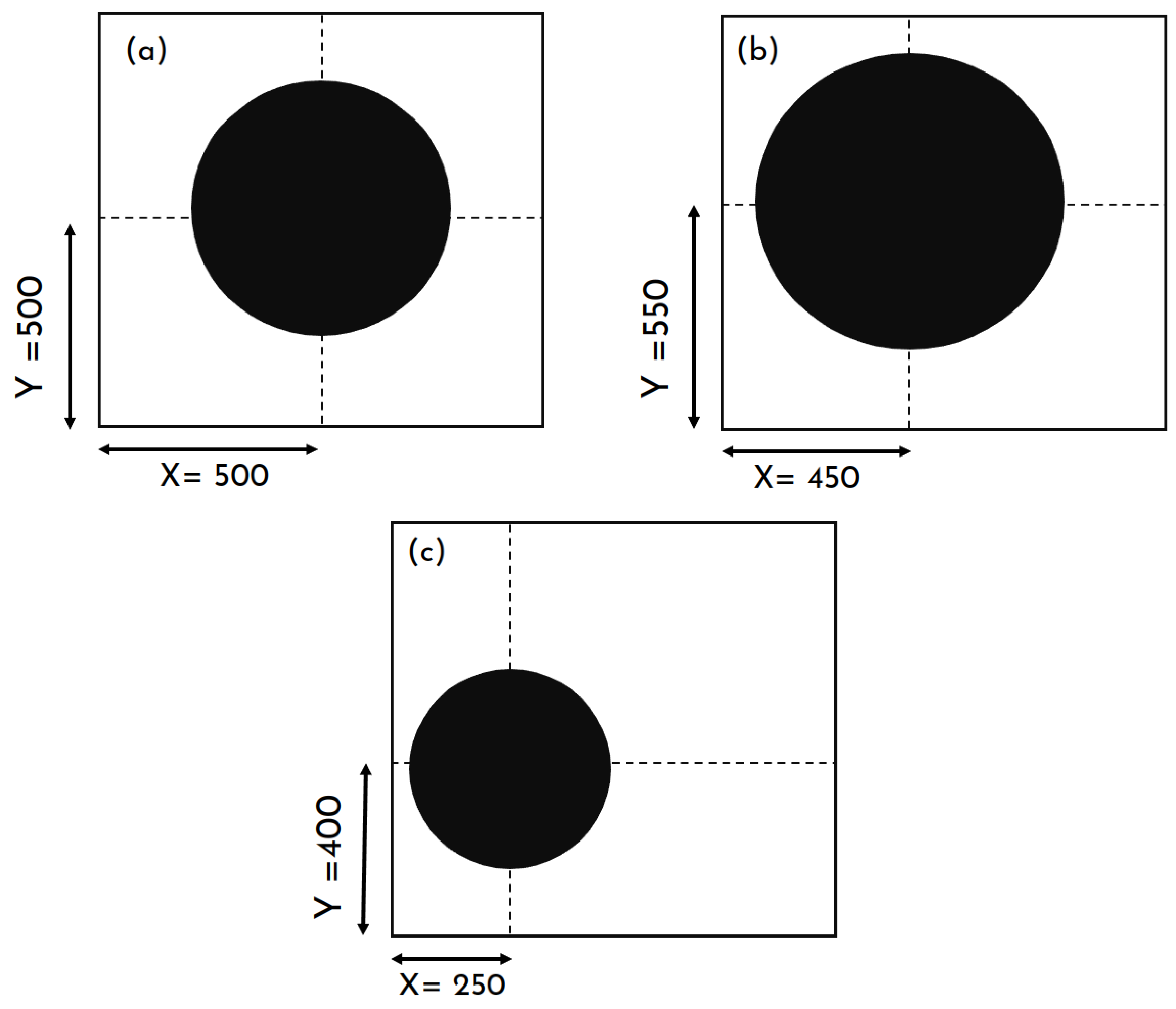
To assess the efficacy of combining machine learning with genetic algorithms to discover equivalent morphologies, diverse scenarios were crafted, as shown in Figure 16, with each manipulating different variables. The initial scenario centers around an inclusion positioned at the center of a 1000 × 1000 matrix that is firmly fixed at coordinates (500, 500). Here, the volume fraction stands at 25% and is accompanied by a contrast of 80 between the two phases. In the subsequent scenario, the inclusion is randomly situated within the matrix, mirroring real-world conditions more closely. With the volume fraction raised to 30% and the contrast lowered to 50, this adjustment evaluates the system’s capability to manage scenarios where the inclusion’s range is constrained and contrasts are less pronounced. Continuing this investigation, the third scenario reduces the volume fraction to 20% and further diminishes the contrast to 20. The inclusion’s placement remains randomized, reflecting scenarios where inclusion characteristics may be less defined. Each scenario is meticulously designed to scrutinize the ML-GA coupling’s aptitude in recognizing equivalent morphologies across a spectrum of conditions, spanning from ideal scenarios to more intricate and realistic environments.

Scenario A:

-

Inclusion position: centered inclusion with coordinates (500, 500);

-

Volume fraction $V_f$: 25%;

-

Contrast C: 80.

Scenario B:

-

Inclusion position: randomly placed with coordinates (450, 550);

-

Volume fraction $V_f$: 30%;

-

Contrast C: 50.

Scenario C:

-

Inclusion position: randomly placed with coordinates (250, 400);

-

Volume fraction $V_f$: 20%;

-

Contrast C: 20

Interpretation

Figure 17 below illustrates the results obtained from various scenarios explored by the coupling model. Each scenario corresponds to a specific geometric configuration of the inclusion, thus influencing its behavior within the matrix. In the first scenario, where the inclusion is a centered circle, a unique solution is identified in the database. However, finding an equivalent morphology proves to be complex. Despite this, the model manages to discover a satisfactory solution with adaptation values close to one. This adequacy is particularly remarkable in the elliptical case, with a shape ratio of 2/3, as well as in the square case, for which the shape is similar to that of a circle. Other solutions were found with less adaptation in the elliptical case (aspect ratio = 1/2) and triangular case, but they had even lower adaptation in the case of an elongated elliptical inclusion (aspect ratio = 1/3), where the shape is far from circular, and where the degree of freedom in the matrix is limited. In the second scenario, where the volume fraction is fixed at 30%, the solutions do not differ considerably from those of the first scenario. This is because the inclusion has less freedom in the matrix, restricting the set of possible solutions. Conversely, in scenario C, where the volume fraction is reduced to 20% and the inclusion is randomly positioned, the solutions show increased accuracy. The adaptation values range between 0.86 and 0.98. This improvement is attributable to the greater freedom granted to the inclusion, promoting a more homogeneous distribution within the matrix.

In the second figure (Figure 18), we scrutinize the outcomes derived from employing a secondary coupling model predicated on an artificial neural network. This model is specifically tailored to seek analogous morphological representations within the identical database as the input configuration. To ensure exhaustive exploration of the solution space, we implement a penalization algorithm. This mechanism, coupled with the stipulation of a fixed quantity of solutions for exploration, facilitates the generation of multiple potential solutions subsequent to each instance of penalization.

Upon meticulous examination of the results, we observe that the coupling model exhibits commendable efficacy across all scrutinized scenarios (A, B, and C). The obtained adaptation values fall within the range of 0.94 to 0.99, affirming the efficacy of the adopted coupling methodology. This substantiates the model’s adeptness in accurately delineating intricate interrelations among diverse variables and the corresponding fine-tuning of the model’s parameters.

Nevertheless, it is imperative to underscore that the adaptation value undergoes diminution following each penalization iteration. This decline can be attributed to the excision of previously identified solutions. This iterative culling process, which is aimed at eliminating suboptimal solutions while accentuating more promising ones, facilitates the convergence of the model towards more resilient configurations that better align with observed data.

The integration of machine learning models and genetic algorithms presents a hopeful avenue for identifying equivalent morphologies within microstructures housing circular inclusions. This hybrid approach harnesses the respective advantages of each technique: machine learning’s capacity to discern significant patterns from data and genetic algorithms’ prowess in optimization. Yet obstacles like the intricate shapes of inclusions and constraints posed by elevated volume fractions may result in fitness values diverging from ideal outcomes. Nonetheless, the method’s efficacy in confronting these hurdles and furnishing a structured framework for microstructural analysis remains unequivocal.

5. Conclusions

In this study, we developed a novel methodology aimed at discerning equivalent morphologies within a microstructure housing a circular inclusion. Our approach relies on a comprehensive analysis of the microstructure’s linear elastic and thermal behavior, which is facilitated by a coupling model integrating machine learning methodologies with genetic algorithms.

Our investigative process commenced with meticulous data acquisition. We systematically generated a range of microstructures embodying diverse inclusion shapes such as circles, ellipses, squares, and triangles: each characterized by a varying volume fraction $V_f$ and contrast value C. The overarching goal was to assemble a robust database representative of the manifold structures encountered in practical scenarios.

Subsequently, this dataset served as the foundation for determining key mechanical properties: namely, the bulk and shear moduli and the thermal conductivity. This task was accomplished through the utilization of finite element simulation techniques, which afford precise insights into the mechanical and thermal responses of the microstructures under consideration.

The assembled dataset was then partitioned into two distinct subsets. The first subset comprises data subsets corresponding to each inclusion shape, with fixed $V_f$ and C values, serving as inputs for an XGBoost machine learning model. The second subset encompasses circular microstructures, exhibiting variations in $V_f$ and C, to train an artificial neural network model with integrated dropout layers to mitigate overfitting. Both developed models demonstrated promising predictive capabilities, significantly streamlining the task of genetic algorithms. Leveraging the prescribed input microstructure parameters, these algorithms yielded two distinct outcomes: first, the generation of morphologies with equivalent mechanical properties, characterized by comparable fractions and contrasts but differing inclusion geometries; second, the synthesis of circular microstructures exhibiting variations in $V_f$ and C values.

The outcomes of our study substantiate the effectiveness of the proposed methodology in tackling the multifaceted challenge at hand. Particularly noteworthy is the commendable adaptation observed across pivotal mechanical moduli—namely, the bulk modulus, shear modulus, and thermal conductivity. This underscores the significance and efficacy of amalgamating machine learning methodologies with genetic algorithms in the composite materials field.