Author Contributions
Conceptualization, A.R.; methodology, A.R. and N.A.-Y.; validation, A.R. and N.A.-Y.; formal analysis, A.R. and N.A.-Y.; investigation, N.A.-Y.; resources, A.R.; data curation, N.A.-Y.; writing—original draft preparation, N.A.-Y.; writing—review and editing, A.R. and N.A.-Y.; visualization, N.A.-Y.; supervision, A.R.; project administration, A.R.; funding acquisition, A.R. All authors have read and agreed to the published version of the manuscript.
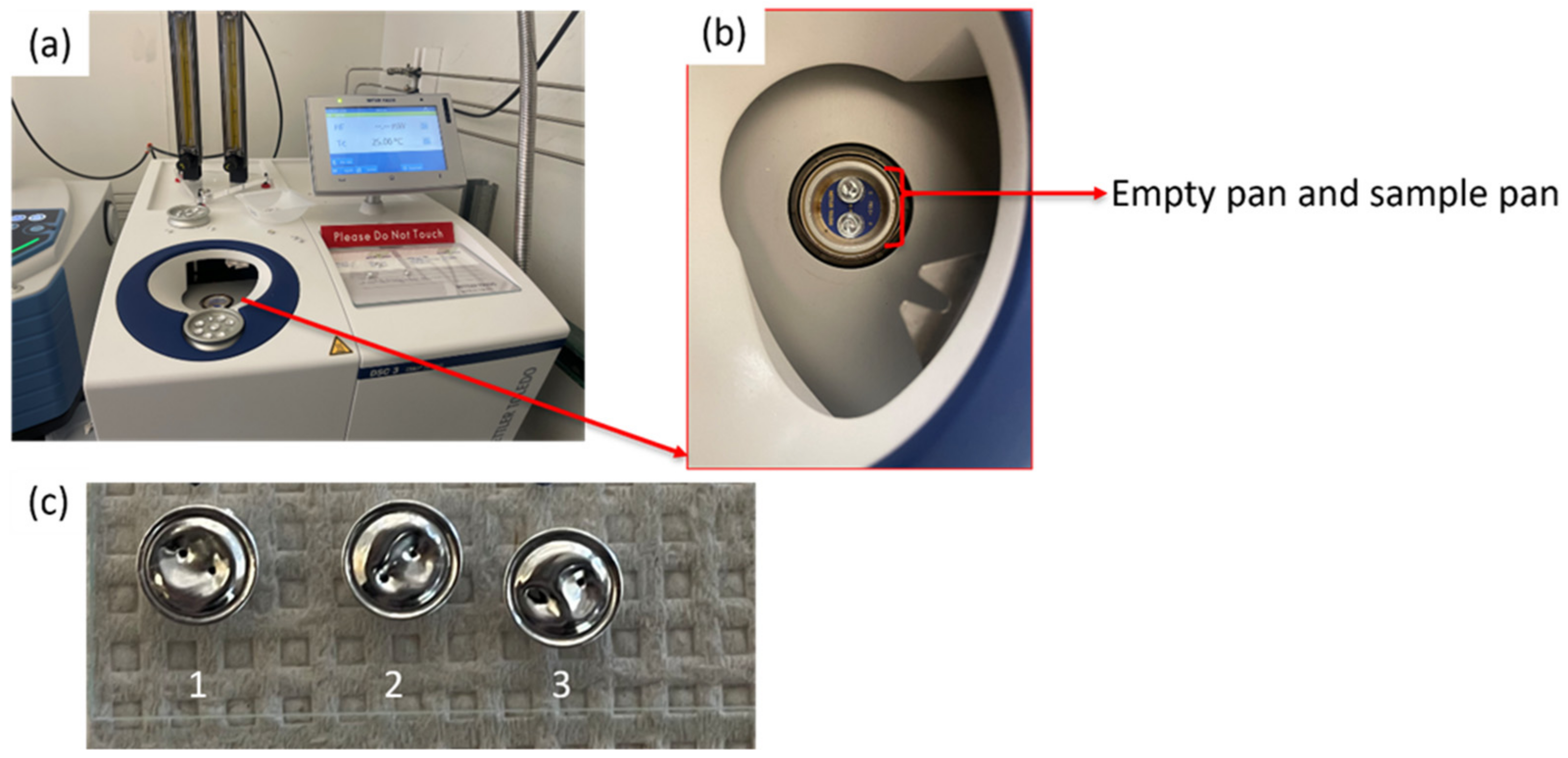
Figure 1.
Digital images showing (a) Mettler Toledo High DSC 3 used for measuring the specific heat capacity of CMF up to 400 °C; (b) empty pan and sample pan slots; (c) three samples tested in the crimped pans.
Figure 1.
Digital images showing (a) Mettler Toledo High DSC 3 used for measuring the specific heat capacity of CMF up to 400 °C; (b) empty pan and sample pan slots; (c) three samples tested in the crimped pans.
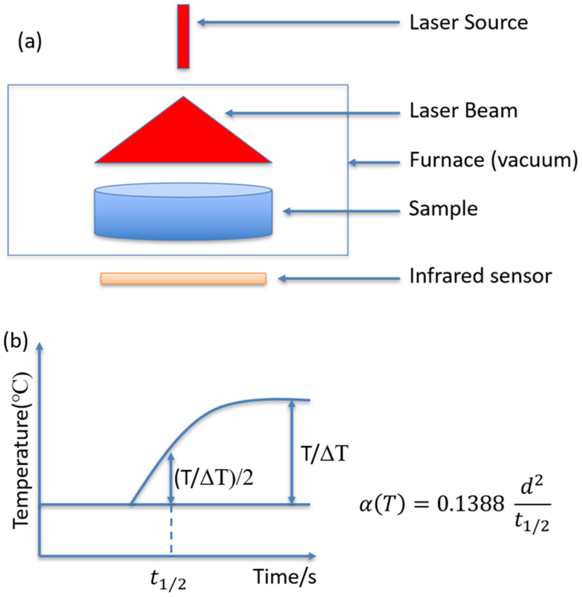
Figure 2.
(a) Schematic showing laser flash technique principle; (b) Parker’s relationship.
Figure 2.
(a) Schematic showing laser flash technique principle; (b) Parker’s relationship.
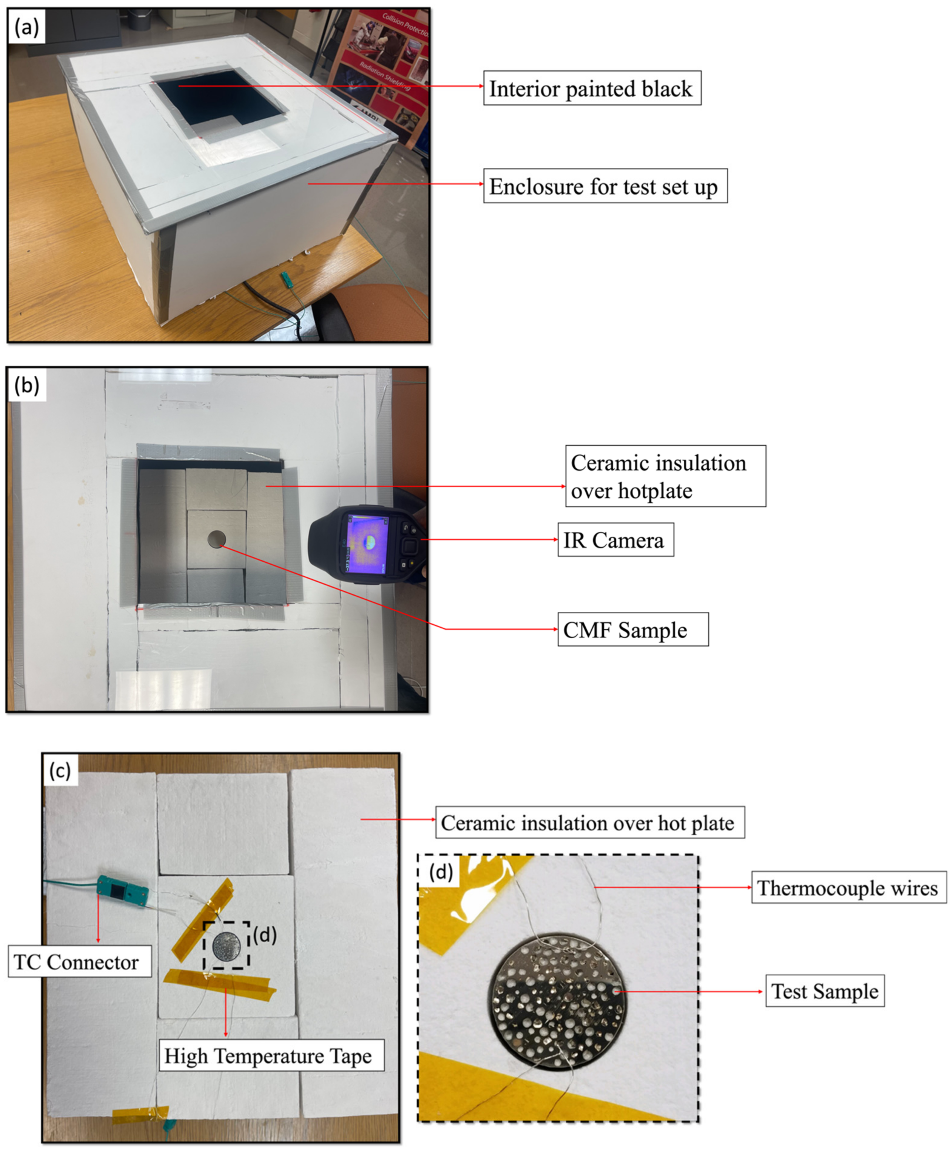
Figure 3.
(a) Overview of the surface emissivity test setup; (b) IR camera for measuring emissivity; (c) ceramic insulation on a hot plate with CMF inserted to its center; (d) CMF sample with a thermocouple on the surface.
Figure 3.
(a) Overview of the surface emissivity test setup; (b) IR camera for measuring emissivity; (c) ceramic insulation on a hot plate with CMF inserted to its center; (d) CMF sample with a thermocouple on the surface.
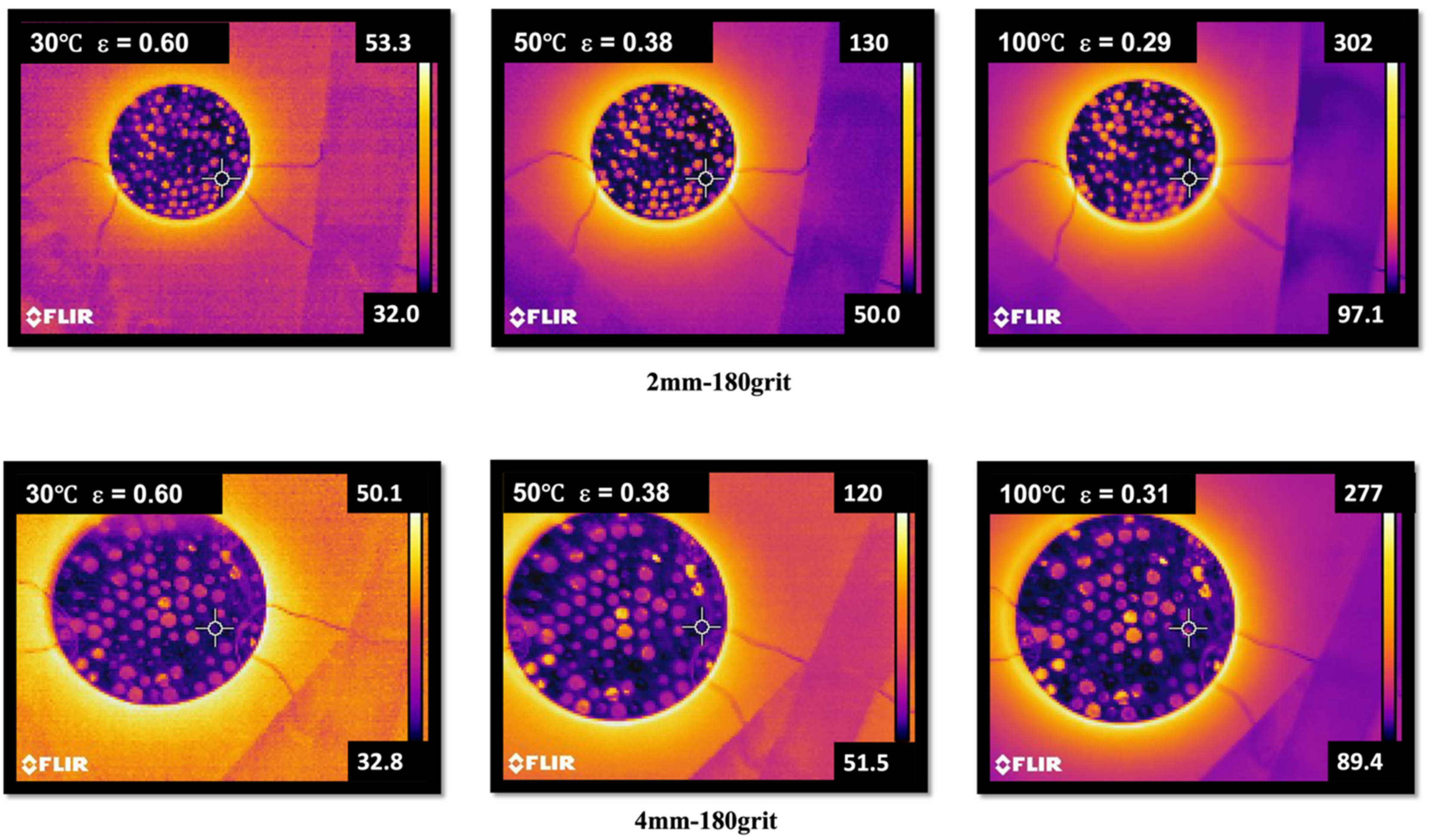
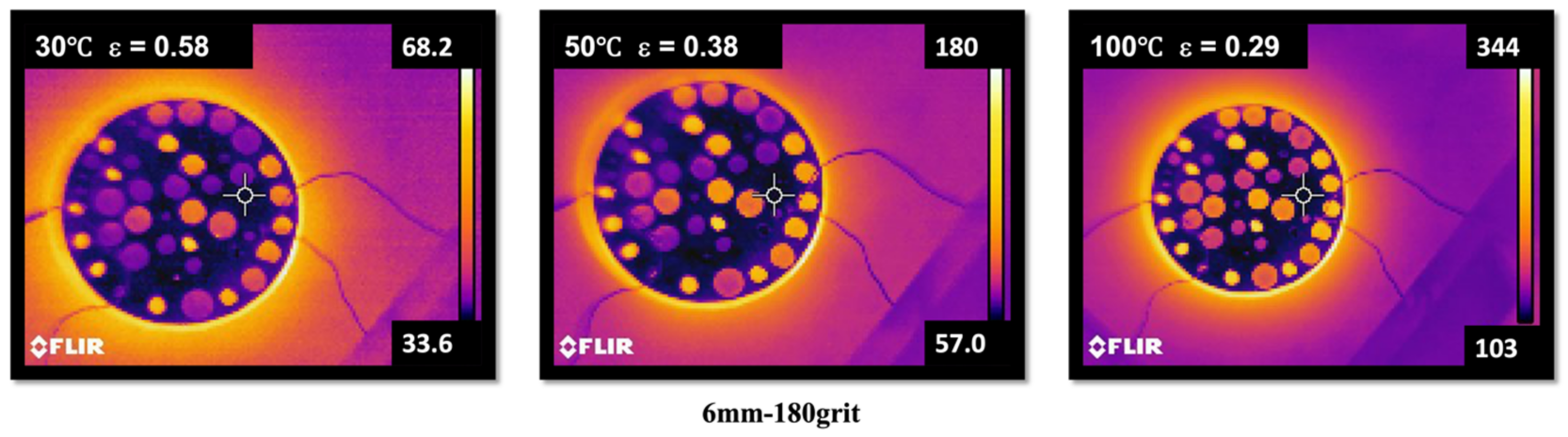
Figure 4.
IR camera readings for 2 mm, 4 mm and 6 mm-sphered CMF samples with 180-grit roughness at 30 °C, 50 °C and 100 °C, showing the change in emissivity.
Figure 4.
IR camera readings for 2 mm, 4 mm and 6 mm-sphered CMF samples with 180-grit roughness at 30 °C, 50 °C and 100 °C, showing the change in emissivity.
Figure 5.
Schematic showing (a) comparison between IR camera beam capturing internal surface of a sphere (A) as opposed to capturing sphere and matrix due to smaller size of the exposed sphere (B). (b) Side-view schematic showing the cross-section passing through line CC with depth cap of spheres measured as Z1 and Z2.
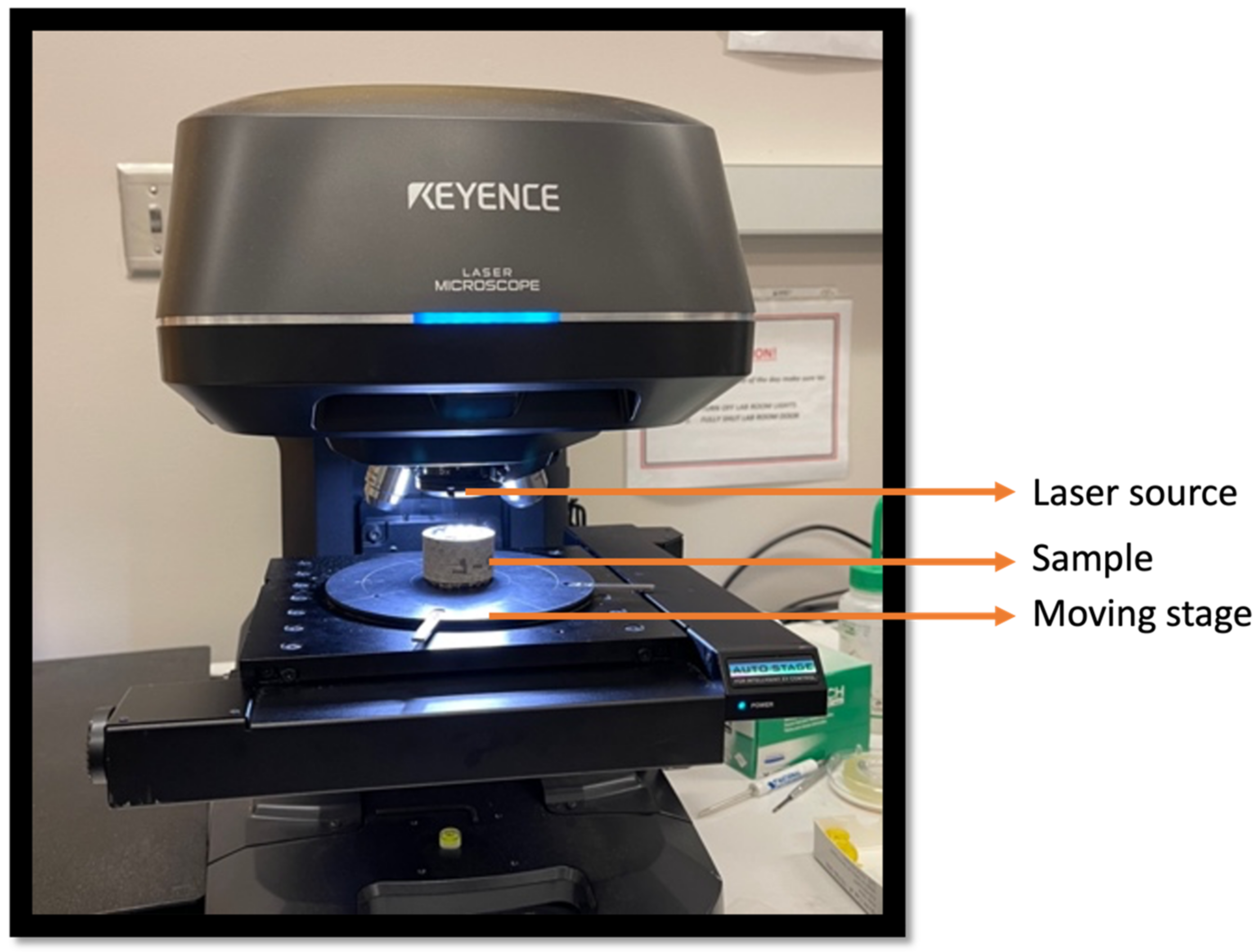
Figure 6.
Keyence VKx110 optical profilometer scanning CMF sample for surface roughness.
Figure 6.
Keyence VKx110 optical profilometer scanning CMF sample for surface roughness.
Figure 7.
Keyence VKx1100 optical image of one sphere within the CMF and 3D rendering of the scanned sphere and its surrounding matrix area.
Figure 7.
Keyence VKx1100 optical image of one sphere within the CMF and 3D rendering of the scanned sphere and its surrounding matrix area.
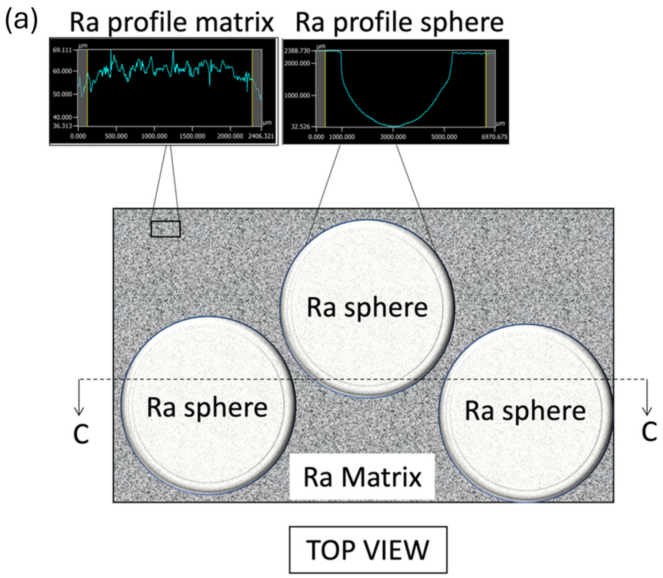
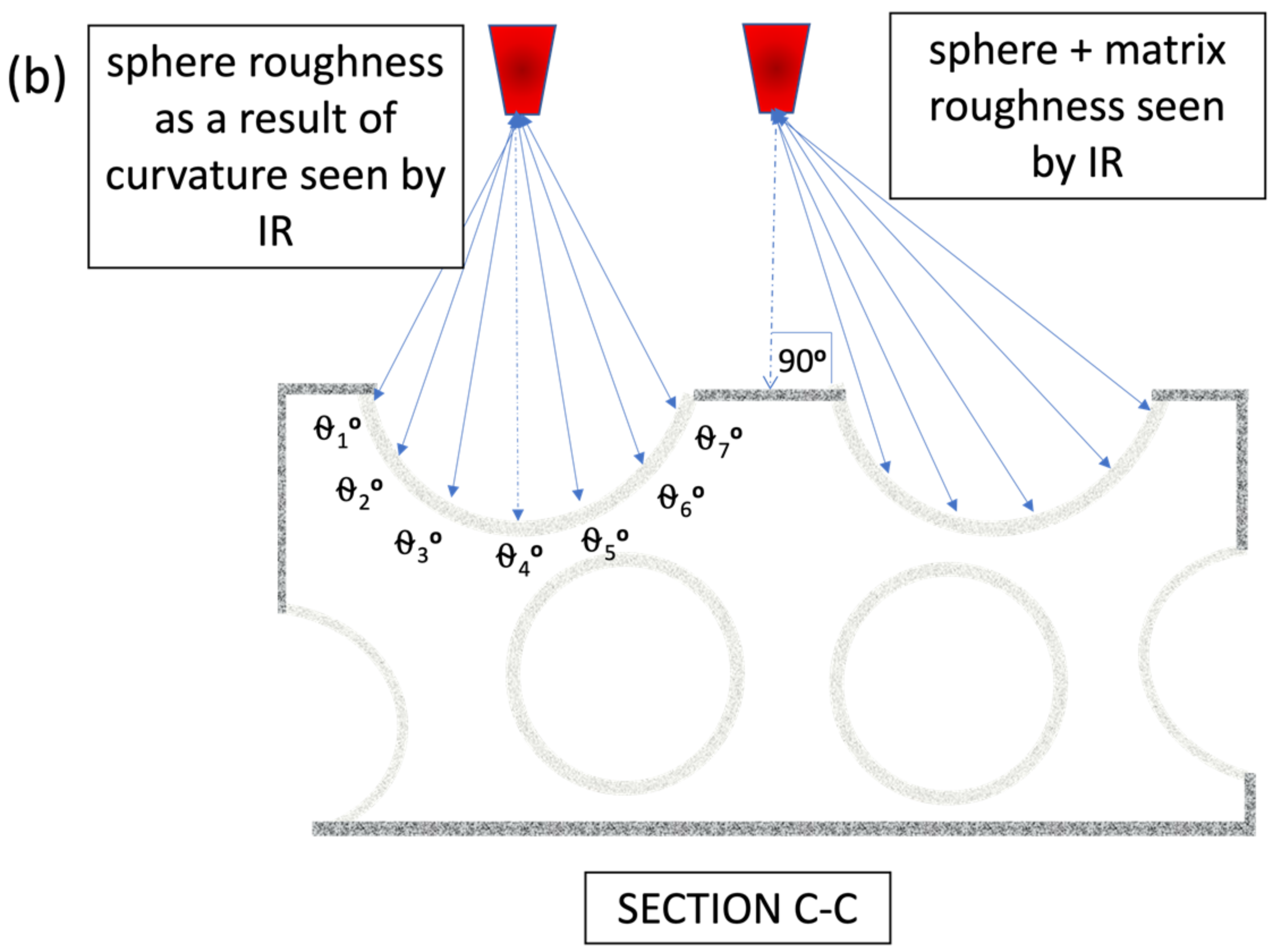
Figure 8.
Schematic showing: (a) Top view of the sphere and matrix roughness distribution on S-S CMF surface. (b) Sectional view of the sample showing IR camera reflection sight for matrix and sphere curvature.
Figure 8.
Schematic showing: (a) Top view of the sphere and matrix roughness distribution on S-S CMF surface. (b) Sectional view of the sample showing IR camera reflection sight for matrix and sphere curvature.
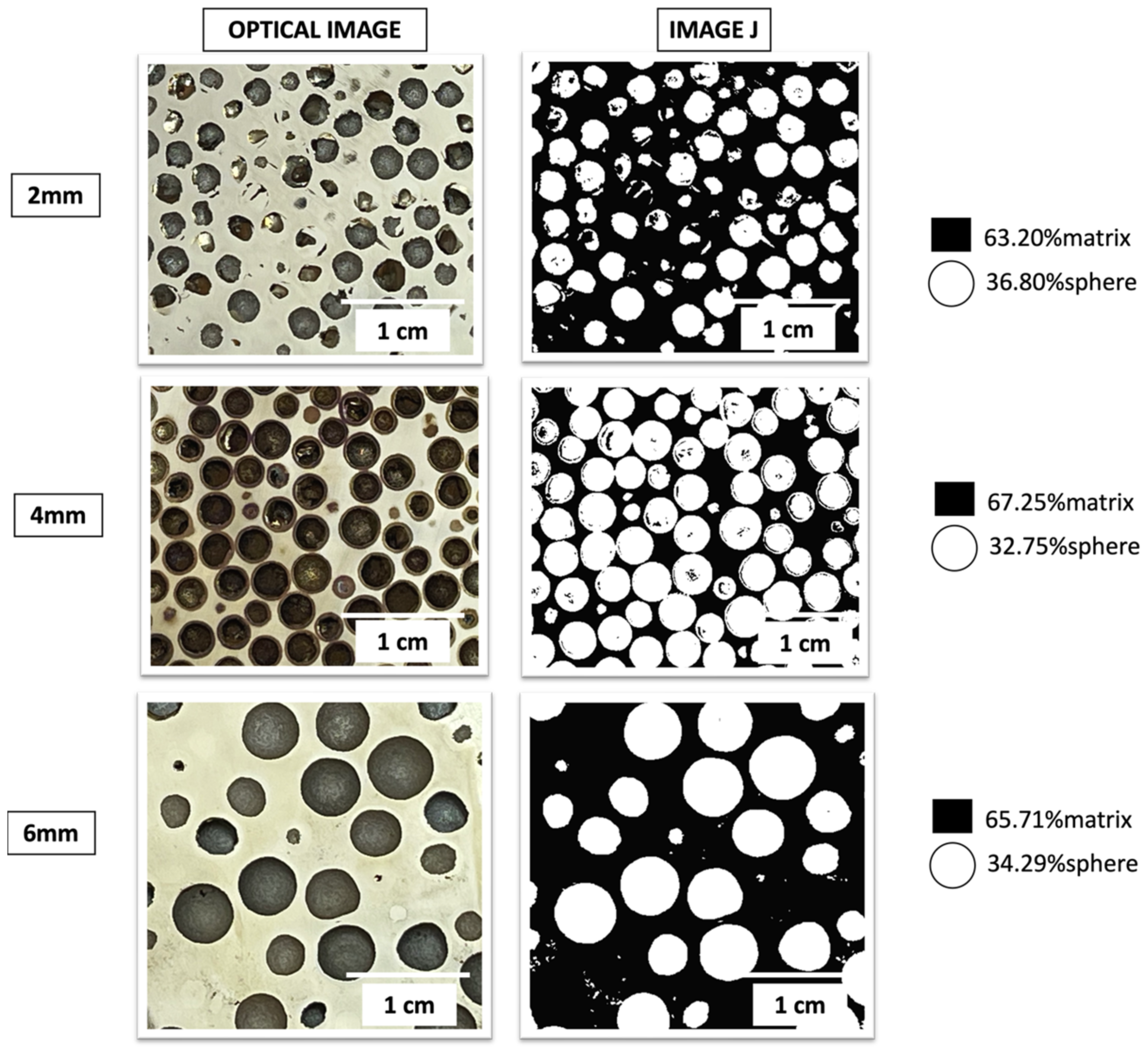
Figure 9.
Optical and ImageJ analysis of the surface area of CMF samples with different sphere sizes of 2 mm, 4 mm and 6 mm.
Figure 9.
Optical and ImageJ analysis of the surface area of CMF samples with different sphere sizes of 2 mm, 4 mm and 6 mm.
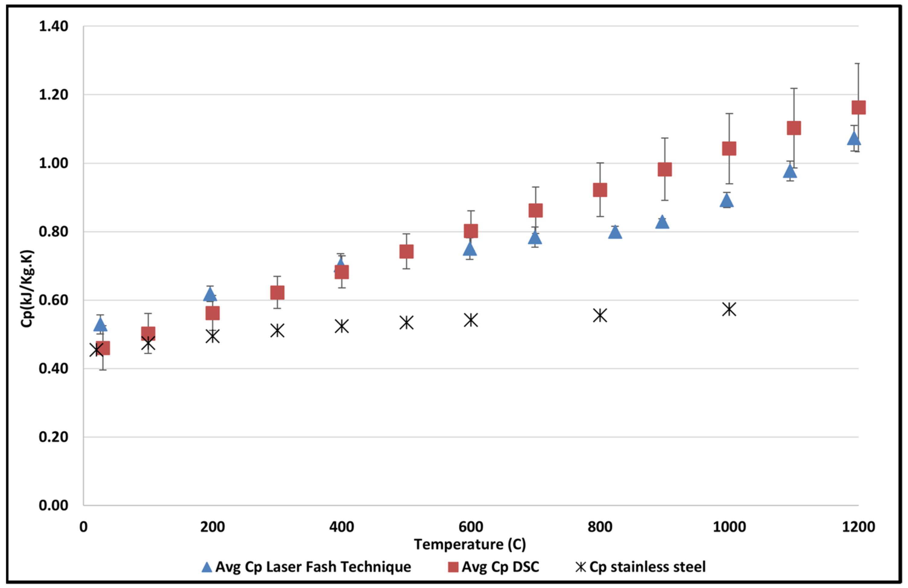
Figure 10.
The specific heat capacity of composite metal foam using laser flash and the DSC technique is in comparison to the specific heat capacity of stainless steel.
Figure 10.
The specific heat capacity of composite metal foam using laser flash and the DSC technique is in comparison to the specific heat capacity of stainless steel.
Figure 11.
Results for the calibration of the test setup, measuring the emissivity of flat 316L stainless steel with various roughness compared to that of 316L emissivity from the literature [
22].
Figure 11.
Results for the calibration of the test setup, measuring the emissivity of flat 316L stainless steel with various roughness compared to that of 316L emissivity from the literature [
22].
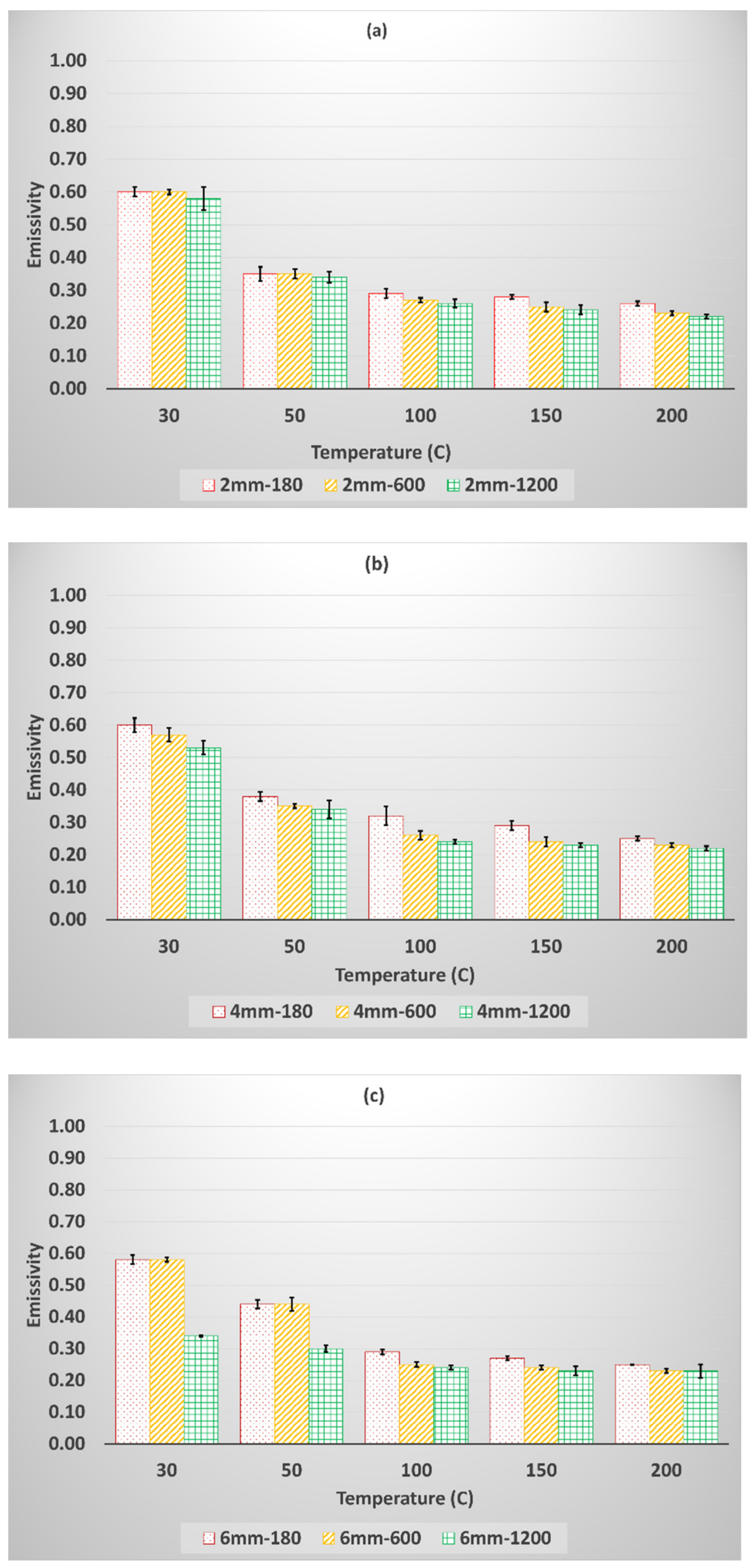
Figure 12.
(a) 2 mm (b) 4 mm (c) 6 mm sphere CMF matrix emissivity values with changing the matrix roughness and test temperatures.
Figure 12.
(a) 2 mm (b) 4 mm (c) 6 mm sphere CMF matrix emissivity values with changing the matrix roughness and test temperatures.
Figure 13.
Directly measured spheres’ emissivity for 2 mm, 4 mm and 6 mm spheres.
Figure 13.
Directly measured spheres’ emissivity for 2 mm, 4 mm and 6 mm spheres.
Figure 14.
Effects of surface curvature on the emissivity of the spheres’ inner surfaces.
Figure 14.
Effects of surface curvature on the emissivity of the spheres’ inner surfaces.
Figure 15.
(a) Experimental and (b) extrapolated upper bound (UB) and lower bound (LB) global emissivity of 2 mm sphered CMF samples, comparing emissivity as a result of effects of sphere curvature (UB-A, LB-A) and as a result of direct measurements (UB-B, LB-B) at various temperatures.
Figure 15.
(a) Experimental and (b) extrapolated upper bound (UB) and lower bound (LB) global emissivity of 2 mm sphered CMF samples, comparing emissivity as a result of effects of sphere curvature (UB-A, LB-A) and as a result of direct measurements (UB-B, LB-B) at various temperatures.
Figure 16.
(a) Experimental and (b) extrapolated upper bound (UB) and lower bound (LB) global emissivity of 4 mm sphered CMF samples, comparing emissivity as a result of effects of sphere curvature (UB-A, LB-A) and as a result of direct measurements (UB-B, LB-B) at various temperatures.
Figure 16.
(a) Experimental and (b) extrapolated upper bound (UB) and lower bound (LB) global emissivity of 4 mm sphered CMF samples, comparing emissivity as a result of effects of sphere curvature (UB-A, LB-A) and as a result of direct measurements (UB-B, LB-B) at various temperatures.
Figure 17.
(a) Experimental and (b) extrapolated upper bound (UB) and lower bound (LB) global emissivity of 6 mm sphered CMF samples, comparing emissivity as a result of effects of sphere curvature (UB-A, LB-A) and as a result of direct measurements (UB-B, LB-B) at various temperatures.
Figure 17.
(a) Experimental and (b) extrapolated upper bound (UB) and lower bound (LB) global emissivity of 6 mm sphered CMF samples, comparing emissivity as a result of effects of sphere curvature (UB-A, LB-A) and as a result of direct measurements (UB-B, LB-B) at various temperatures.
Figure 18.
Comparison of the emissivity obtained for 2 mm CMF in this study using the previous experimental emissivity measurement of 2 mm S-S CMF [
16].
Figure 18.
Comparison of the emissivity obtained for 2 mm CMF in this study using the previous experimental emissivity measurement of 2 mm S-S CMF [
16].
Table 1.
Chemical composition of S-S CMF components by weight percent.
Table 1.
Chemical composition of S-S CMF components by weight percent.
| | Chemical Composition (Weight Percent) |
|---|
| Material | Fe | C | Mn | Si | Cr | Ni | Mo |
|---|
| Stainless Steel Hollow Spheres | Balance | 0.68 | 0.13 | 0.82 | 16.11 | 11.53 | 2.34 |
| 316L Steel Matrix | Balance | 0.03 | 2.00 | 1.00 | 16.00–18.00 | 10.00–14.00 | 2.00–3.00 |
Table 2.
CMF sample mass is used to measure the specific heat capacity (Cp) via the DSC method.
Table 2.
CMF sample mass is used to measure the specific heat capacity (Cp) via the DSC method.
| | Sample Mass for Cp Measurement via DSC Technique |
|---|
| Sample number | 1 | 2 | 3 |
| Mass (mg) | 10.1 | 18.7 | 16.0 |
Table 3.
CMF sample dimensions for Cp measurements using laser flash technique.
Table 3.
CMF sample dimensions for Cp measurements using laser flash technique.
| Sample Number | Sample Dimensions for Laser Flash Technique |
|---|
| Diameter (mm) | Thickness (mm) | Density (g/cm3) |
|---|
| 1 | 25.3 | 5.96 | 2.63 |
| 2 | 25 | 5.72 | 2.56 |
| 3 | 25 | 5.91 | 2.68 |
Table 4.
Dimensions of cylindrical S-S CMF samples used for emissivity tests.
Table 4.
Dimensions of cylindrical S-S CMF samples used for emissivity tests.
| Sample | Sample Diameter (mm) | Sample Height (mm) |
|---|
| 2 mm—sphered S-S CMF | 25.59 | 25.26 |
| 4 mm—sphered S-S CMF | 38.24 | 25.28 |
| 6 mm—sphered S-S CMF | 37.61 | 25.21 |
Table 5.
Specific heat capacity results for steel–steel CMF at various temperatures using the DSC technique. Note that the actual data are highlighted in Bold Italic font, and the remaining data are a result of extrapolation.
Table 5.
Specific heat capacity results for steel–steel CMF at various temperatures using the DSC technique. Note that the actual data are highlighted in Bold Italic font, and the remaining data are a result of extrapolation.
| Nominal Temperature (°C) | Specific Heat Capacity Using DSC (kJ/Kg·K) |
|---|
| Sample 1 | Sample 2 | Sample 3 | Average |
|---|
| 30 | 0.49 | 0.37 | 0.52 | 0.46 |
| 100 | 0.53 | 0.42 | 0.55 | 0.50 |
| 200 | 0.60 | 0.49 | 0.59 | 0.56 |
| 300 | 0.67 | 0.56 | 0.63 | 0.62 |
| 400 | 0.74 | 0.63 | 0.67 | 0.68 |
|
500
|
0.81
|
0.70
|
0.71
|
0.74
|
| 600 | 0.88 | 0.77 | 0.75 | 0.80 |
| 700 | 0.95 | 0.84 | 0.79 | 0.86 |
| 800 | 1.02 | 0.91 | 0.83 | 0.92 |
| 900 | 1.09 | 0.98 | 0.87 | 0.98 |
| 1000 | 1.16 | 1.05 | 0.91 | 1.04 |
| 1100 | 1.23 | 1.12 | 0.95 | 1.10 |
| 1200 | 1.30 | 1.19 | 0.99 | 1.16 |
Table 6.
Specific heat capacity results for steel–steel CMF at various temperatures using laser flash technique.
Table 6.
Specific heat capacity results for steel–steel CMF at various temperatures using laser flash technique.
| Nominal Temp (°C) | Specific Heat Capacity Using Laser Flash Technique (kJ/Kg.K) |
|---|
| Sample 1 | Sample 2 | Sample 3 | Average |
|---|
| 26 | 0.491 | 0.556 | 0.541 | 0.529 |
| 200 | 0.59 | 0.617 | 0.646 | 0.618 |
| 400 | 0.661 | 0.703 | 0.742 | 0.702 |
| 600 | 0.707 | 0.762 | 0.782 | 0.75 |
| 700 | 0.743 | 0.799 | 0.81 | 0.784 |
| 823 | 0.778 | 0.812 | 0.81 | 0.8 |
| 900 | 0.829 | 0.818 | 0.84 | 0.829 |
| 1000 | 0.865 | 0.919 | 0.893 | 0.892 |
| 1100 | 0.972 | 1.015 | 0.944 | 0.977 |
| 1200 | 1.02 | 1.101 | 1.098 | 1.073 |
Table 7.
Measured sphere surface roughness (Ra) values for various steel CMF samples.
Table 7.
Measured sphere surface roughness (Ra) values for various steel CMF samples.
| Sample | 2 mm-Sphered | 4 mm-Sphered | 6 mm-Sphered | Flat 316L Steel |
|---|
| Ra (μm) | 5.58 | 5.82 | 5.62 | 5.69 |
| Standard Deviation | 1.54 | 0.68 | 0.54 | 0.26 |
Table 8.
Emissivity measurements obtained for a flat 316L stainless steel sample mimicking the inner surface of spheres.
Table 8.
Emissivity measurements obtained for a flat 316L stainless steel sample mimicking the inner surface of spheres.
| Temperature (°C) | Emissivity |
|---|
| 50 | 0.8 |
| 100 | 0.8 |
| 150 | 0.75 |
| 200 | 0.63 |
| 250 | 0.58 |
Table 9.
Average calculated emissivity values of 2 mm, 4 mm and 6 mm hollow steel spheres in the CMF samples based on the sphere’s inner curvature at various temperatures.
Table 9.
Average calculated emissivity values of 2 mm, 4 mm and 6 mm hollow steel spheres in the CMF samples based on the sphere’s inner curvature at various temperatures.
| | Emissivity | |
|---|
| Temperature (°C) | 2 mm | 4 mm | 6 mm | Average | Deviation |
|---|
| 50 | 0.765 | 0.808 | 0.761 | 0.778 | ±0.026 |
| 101 | 0.745 | 0.807 | 0.782 | 0.778 | ±0.031 |
| 152 | 0.702 | 0.756 | 0.726 | 0.728 | ±0.027 |
| 203 | 0.601 | 0.612 | 0.611 | 0.608 | ±0.006 |
| 248 | 0.531 | 0.563 | 0.58 | 0.558 | ±0.025 |
Table 10.
Standard uncertainties or ranges of the input quantities.
Table 10.
Standard uncertainties or ranges of the input quantities.
Table 11.
Average emissivity values for various sphere-sized CMF samples.
Table 11.
Average emissivity values for various sphere-sized CMF samples.
| | 2 mm-CMF | 4 mm-CMF | 6 mm-CMF |
|---|
| Temperature (°C) | Sphere | Matrix | Sphere | Matrix | Sphere | Matrix |
|---|
| εs | εm | εs | εm | εs | εm |
|---|
| 50 | 0.71 | 0.58 | 0.71 | 0.53 | 0.66 | 0.3 |
| 75 | 0.7 | 0.34 | 0.69 | 0.34 | 0.64 | 0.26 |
| 100 | 0.68 | 0.26 | 0.67 | 0.24 | 0.57 | 0.24 |
| 150 | 0.59 | 0.24 | 0.64 | 0.23 | 0.49 | 0.23 |
| 200 | 0.57 | 0.22 | 0.63 | 0.22 | 0.46 | 0.23 |
Table 12.
Calculated combined standard uncertainties for global CMF emissivity.
Table 12.
Calculated combined standard uncertainties for global CMF emissivity.
| | 2 mm Sample | 4 mm Sample | 6 mm Sample |
|---|
| Temperature (°C) | Emissivity | Equation (5) | MC a | Emissivity | Equation (5) | MC a | Emissivity | Equation (5) | MC a |
|---|
| RT | 0.63 | ±0.0017 | ±0.0013 | 0.59 | ±0.0003 | ±0.0012 | 0.42 | ±0.0006 | ±0.0009 |
| 75 | 0.47 | ±0.0014 | ±0.0009 | 0.45 | ±0.0006 | ±0.0009 | 0.39 | ±0.0006 | ±0.0008 |
| 100 | 0.41 | ±0.0138 | ±0.0009 | 0.38 | ±0.0007 | ±0.0008 | 0.35 | ±0.0005 | ±0.0007 |
| 150 | 0.37 | ±0.0006 | ±0.0007 | 0.36 | ±0.0007 | ±0.0007 | 0.32 | ±0.0003 | ±0.0006 |
| 200 | 0.35 | ±0.0006 | ±0.0007 | 0.35 | ±0.0007 | ±0.0007 | 0.31 | ±0.0002 | ±0.0006 |


