Buckling Optimization of Variable Stiffness Composite Panels for Curvilinear Fibers and Grid Stiffeners

Abstract

Automated Fiber Placement (AFP) machines can manufacture composite panels with curvilinear fibers. In this article, the critical buckling load of grid-stiffened curvilinear fiber composite panels is maximized using a genetic algorithm. The skin is composed of layers in which the fiber orientation varies along one spatial direction. The design variables are the fiber orientation of the panel for each layer and the stiffener layout. Manufacturing constraints in terms of maximum curvature allowable by the AFP machine are imposed for both skin and stiffener fibers. The effect of manufacturing-induced gaps in the laminates is also incorporated. The finite element method is used to perform the buckling analyses. The panels are subjected to in-plane compressive and shear loads under several boundary conditions. Optimization results show that the percentage difference in the buckling load between curvilinear and straight fiber panels depends on the load case and boundary conditions.

1. Introduction

The main driver in the development of materials for aerospace structures is weight reduction. Weight savings mean less fuel is required, which results in a higher payload capacity or a longer range of the aircraft. The call for weight reduction in the aerospace industry has led to the increasing use of composite materials due to their high specific strength and stiffness. Traditionally, composites are made of straight fibers. The fiber angle orientation is uniform, resulting in Constant Stiffness (CS) laminates. Recent advances in manufacturing technology have made it possible to steer the fibers [1]. Laminates composed of plies in which the fiber orientation continuously varies can be manufactured using Automated Fiber Placement (AFP), filament winding (FW) and tailored fiber placement (TFP). Several studies recently investigated the design optimization, manufacturing and testing of variable-fiber angle composite structures considering FW [2,3,4], TFP [5,6] and AFP [7,8,9]. This study focuses a methodology to optimize the variable-angle composite panels manufactured via AFP. It is also feasible to manufacture curvilinearly grid-stiffened panels for enhanced structural performance. Therefore, the stiffness of those composite panels is not constant and depends on the spatial location. The design space is enlarged and substantial improvements in structural performance or weight savings can be obtained [10]. These panels can be employed to manufacture wing or fuselage skins. Skins are thin-walled structures subjected to in-plane loads and are prone to buckling.

In the literature, different approaches have been adopted to define the fiber paths of Variable Stiffness (VS) laminates. Olmedo and Gürdal [1] introduced the linear variation of the fiber angle along one spatial direction to describe curvilinear fiber paths. Substantial improvements in the buckling load over straight fiber laminates were found. Wu et al. [11] defined the fiber angles based on a nonlinear distribution and applied the Rayleigh–Ritz method to perform the buckling analysis of VS panels. S. Ijsselmuiden [12] employed lamination parameters to describe the structural stiffness of VS laminates. This approach decreased the number of design variables, however, a postprocessing step was necessary to convert the optimal lamination parameters into continuous fiber paths.

Gaps and overlaps are induced during manufacturing of a variable stiffness laminate using AFP machine. The study of the influence of those defects on the laminate structural performance has attracted the interest of many authors. A. Blom et al. [13] developed a Finite Element Model (FEM) in which the elements were assumed to be either in ‘regular’ composite zones or in gap zones (characterized by resin properties). It was concluded that a larger gap area decreased the laminate strength and stiffness. Fayazbakhsh et al. [14] modeled VS laminates with embedded defects by computing the percentage of the defect area within an element. The gap area was used to scale the material properties while the overlap area scaled the thickness. In their work, the results showed that gaps degraded in-plane stiffness and buckling load while overlaps improved them. T.Brooks et al. [15] linked the gap/overlap propagation rate and the divergence of a 2D vector field. A positive divergence implied gap formation, while a negative value indicated overlap formation.

The structural performance can be enhanced through grid-stiffened composite skins. Typically, orthogrid or isogrid panels in which the stiffeners follow straight paths are used. However, curvilinearly grid-stiffened layouts offer greater design space by tailoring the location and shape of the stiffeners. Several authors [16,17,18,19] used the linear variation of the fiber angle to define the stiffener paths. The stiffness distribution of the panel was influenced by the angle variation and the distance between the stiffeners. Kapania and his co-authors (see [20,21,22]) employed NURBS (Non-Uniform Rational B-Splines) to describe the reference path of curvilinear stiffeners. It was shown that curvilinear stiffeners could result in a better design than straight stiffeners, but not for all load cases and boundary conditions. Other authors [7,23] parametrized the stiffener geometry using Bézier curves. For NURBS and Bézier curves, special attention was required to ensure that the stiffener lied within the panel boundary.

Designing the optimum staking sequence or the optimum stiffener layout and size often results in many local optima [8,21]. In addition, the sensitivity information of the optimization problem is not always easy to compute. Accordingly, evolutionary optimization techniques are an appropriate alternative to overcome these limitations compared to gradient-based optimization. Genetic Algorithms (GA) as an evolutionary optimization method are the most widely adopted for the buckling optimization of VS laminates and/or curvilinearly grid-stiffened panels (see, for instance [9,11,24]).

In this article, an optimization framework has been developed with the aim of designing composite panels with curvilinear fibers and curvilinear stiffeners for maximum buckling performance. Manufacturing constraints in terms of the maximum allowed curvature by the AFP machine have been imposed for both the skin and stiffener fibers. Manufacturing-induced defects in the form of gaps have been also considered in the design phase. Panels under several boundary conditions and load cases have been optimized using Genetic Algorithm. Optimization of straight fiber panels has also been performed to evaluate the difference between the critical buckling loads obtained with straight fiber and curvilinear fiber designs. The article is organized as follows. Section 2 describes the methodology for modeling variable stiffness laminates and for including the effect of gaps in the FE model. This section continues with the geometry parameterization and modeling of curvilinearly grid-stiffened panels. Section 3 presents the optimization framework. Section 4 introduces the case studies and analyzes the results obtained from the optimization. Section 5 discusses the conclusions drawn from the present work.

2. Numerical Modeling

This section describes how composite panels with curvilinear fibers and grid stiffeners are modeled. The FEA commercial software Abaqus is used for generating the Finite Element models and Python scripts are developed to parameterized them. In the present work, a linear buckling analysis is performed in which the first eigenvalue is requested, since it is usually the one of greatest interest. The solver selected to extract the eigenvalue is the Subspace iteration method as it is particularly suited for the calculation of few eigenmodes (less than 20) of large finite element system [25].

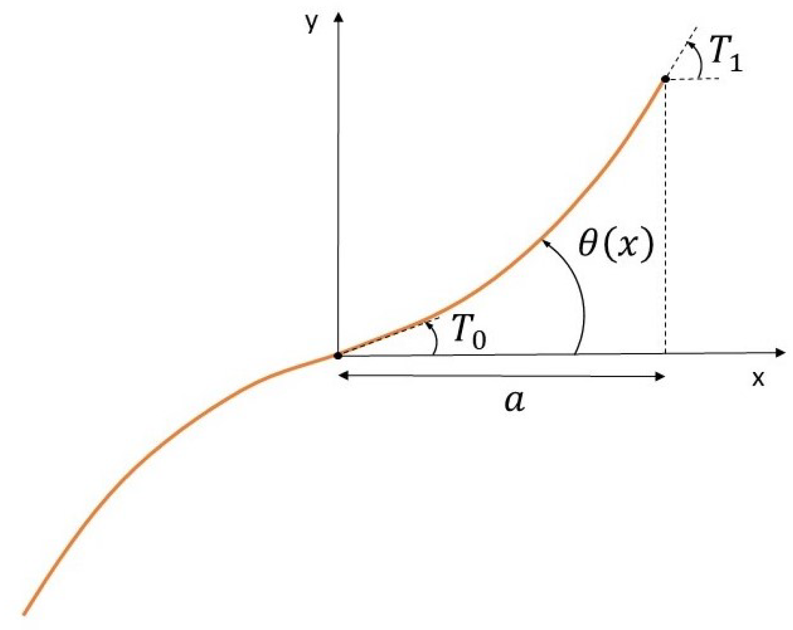
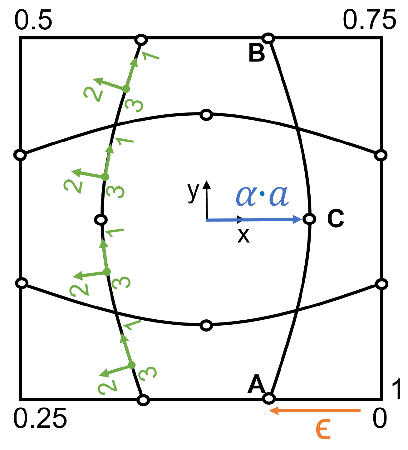
2.1. Curvilinear Skin Fibers

The linear variation of the fiber angle, first introduced by Olmedo and Gürdal [1], has been widely employed to study VS panels due to its simplicity and robustness. Hence, this approach is considered in this work. The fiber angle varies along the x-direction according to Equation (1).

$$\theta \left(x\right)=\left(T_1-T_0\right)\frac{\left|x\right|}{a}+T_0$$

(1)

where $T_0$ and $T_1$ are the fiber angles at the start and end of the characteristic length a; a is considered here as the half side of the square panel. Figure 1 schematized the terms of Equation (1).

At each x-position of the VS ply, the fiber angle is different. The skin is modeled with a suitable number of elements to account for the variation of the fiber angle, i.e., the stiffness. At the centroid of each element, the fiber angle is computed with Equation (1). Since Equation (1) depends on $T_0$ and $T_1$, the variables that characterize a ply, a fiber angle is obtained for each different ply in the laminate. The skin is meshed using $32\times 32$ S4R shell elements. S4R element is a 4-node, quadrilateral, stress-displacement shell element with reduced integration and a large-strain formulation [25].

Figure 2a illustrates the fiber paths for a $〈20,50〉$ ply. Figure 2b shows how the curvilinear fiber paths of the ply are discretized in the FE model. The straight lines represent the fiber angle computed at the centroid of each element.

For straight fiber modeling, it is not necessary to calculate the fiber angle at the centroid of each element, since it is the same for the whole ply. Thus, the local stacking sequence is directly built and assigned to the mesh element.

The Abaqus-Python script developed for modeling CS and VS laminates has been validated with the study presented by Waldhart [26]. The buckling loads for CS and VS laminates were obtained and compared to their results that showed less than 1% error.

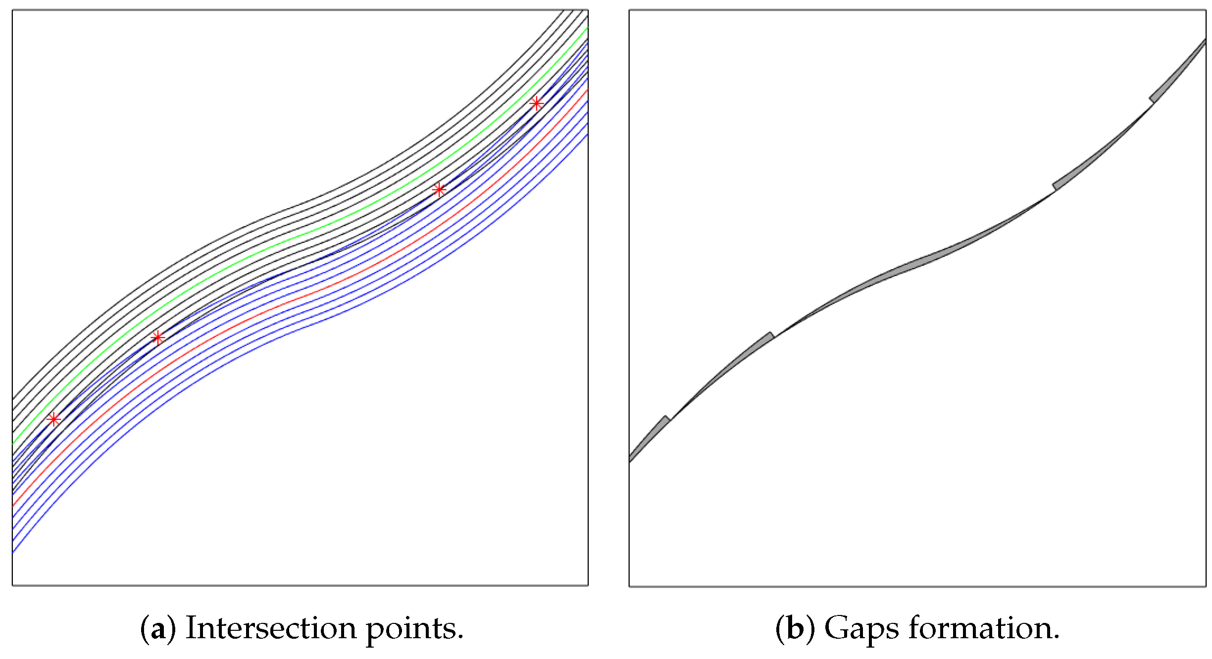
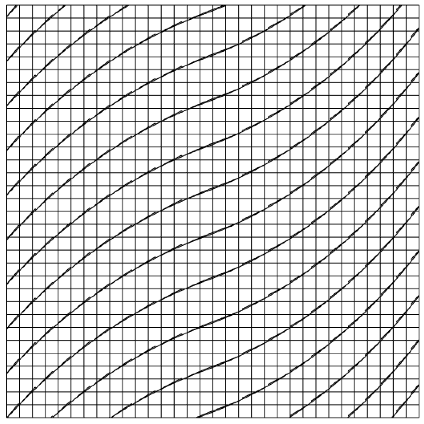
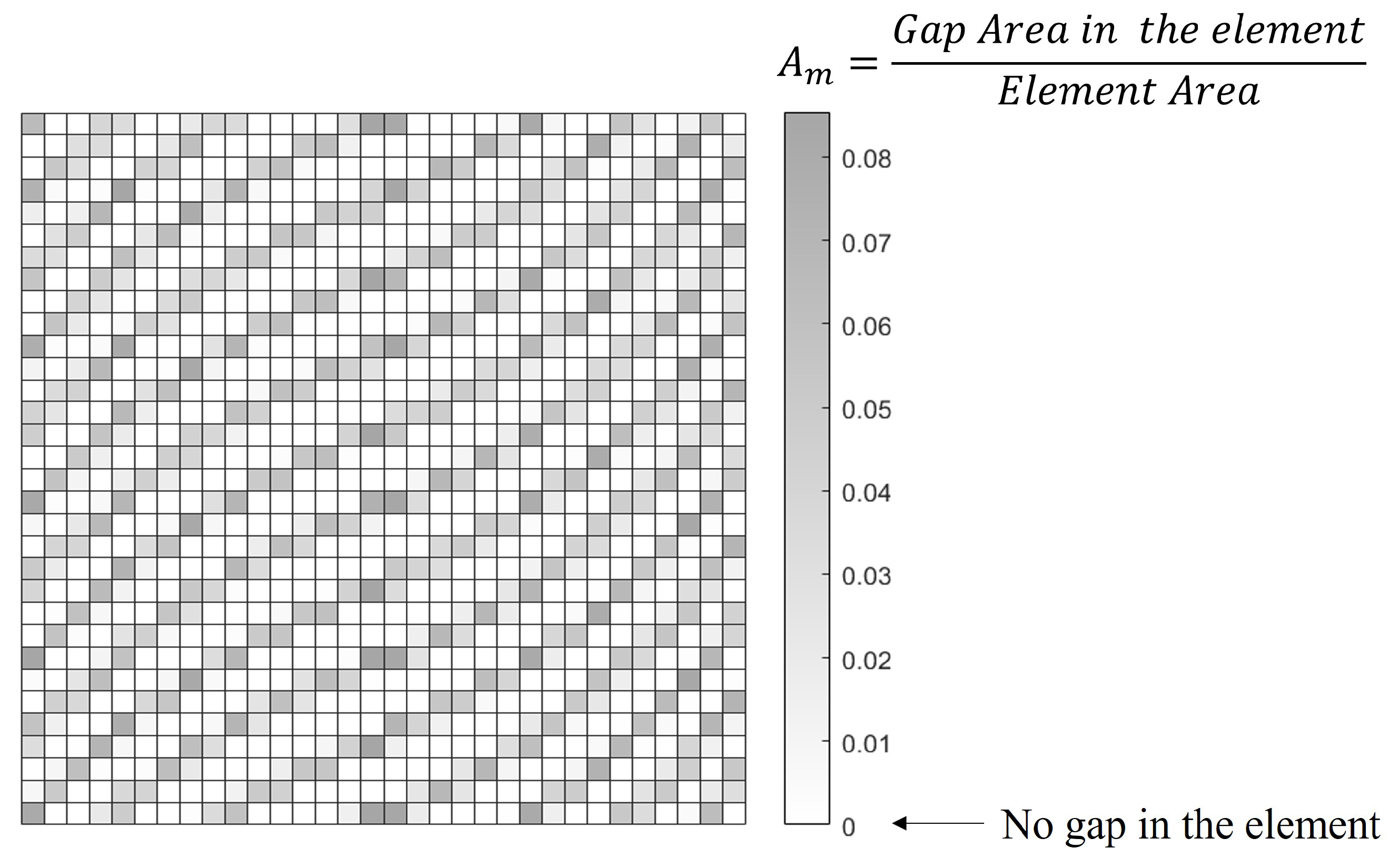
2.2. Modeling of Gaps induced by VS Laminate Manufacturing

Shifted method is used to manufacture variable stiffness laminates in this study. First, the AFP machine deposits the reference course. The distance between the top and bottom boundaries of the course changes along the horizontal direction since the fiber path is curvilinear. The AFP head moves in the vertical direction with a constant value to lay down the next course. If the course width remains constant, large areas of overlap will occur between both courses. Accordingly, the course width should vary continuously. This variation is actually discrete, as the AFP can only cut finite tow widths. Small areas of defects are then generated.

The defects generated can be gaps or overlaps. A gap is a small wedge-shaped without fibers which, after curing, will be filled with resin. An overlap occurs when a small jagged patch of the composite tow lies on top of the adjacent composite course. The 100% coverage or complete overlap strategy has been shown to provide increased structural performance, however, the laminate thickness is not constant. Many aeronautical applications require a smooth surface to maintain aerodynamics, which will not be possible to manufacture with the overlap strategy [14]. Therefore, in this work, 0% coverage or complete gap strategy has been chosen.

One-sided tow drop technique is employed to cut the tows. It implies that one course boundary, either the top or the bottom one, is cut and the other remains smooth.

The approach introduced by Fayazbakhsh et al. [14], called the Defect Layer Method, has been modified to consider the induced gaps when the linear variation of the fiber angle is used to define the fiber paths. A MATLAB code has been developed to locate the gaps in the laminate and obtain their area. Next, the Python script builds the FE model of the VS laminate with embedded gaps.

When the AFP machine deposits the course, its head is perpendicular to the local fiber angle. This means that each point along the AFP head has the same orientation as the one corresponding to the reference path. Thus, the points that form each tow of the course can be calculated by Equation (2).

$$\begin{array}{c}x=x^{*}-i·t_{w}sin{\theta }^{*}\\ y=y^{*}+i·t_{w}cos{\theta }^{*}\end{array}$$

(2)

where $t_w$ is the tow width and $n_t$ the number of tows in a course. The superscript ∗ is used to denote the points in the reference path and i is an index which range decreases by 1 from $n_t/2$ to $-n_t/2$.

The shift distance, i.e., the minimum vertical distance between the top and bottom boundaries of the reference course, is calculated as shown in Equation (3).

$$d_s=min\left(\frac{n_t{t}_w}{cos{\theta }^{*}}\right)$$

(3)

The AFP machine will move vertically with the shift distance to lay down the next course (the shifted course). The points of the shifted course can be obtained by Equation (4).

$$\begin{array}{c}{x}_s=x^{*}-i·t_{w}sin{\theta }^{*}\\ y_s=y^{*}+i·t_{w}cos{\theta }^{*}+d_s\end{array}$$

(4)

The intersections between the outer top edge of the reference course and the tows of the shifted course are next located. A perpendicular line is drawn from each intersection point up to the next corresponding tow edge, reproducing the tow cut made by the AFP machine. Figure 3a shows the intersection points between the shifted course and the reference course. Figure 3b depicts the gap set generated due to that intersection.

The distance between two sets of gaps is the shift distance and, thus, the gap set is translated vertically to generate the defects across the entire ply. The gap distribution is then intersected with the skin mesh to calculate the gap area within an element. Figure 4 illustrates the intersection between the skin mesh and the gaps generated in the ply.

The gaps are resin rich areas, so a higher value of gap area means a decrease in the material properties of the laminate. The ’modified’ rule of mixtures (Equations (5)–(8)) is used to scale the elastic properties of each element according to the gap area fraction. The gap area fraction is defined as the value of the gap area in each element divided by the area of the mesh element.

$$E_1=A_c{E}_{1c}+A_m{E}_m$$

(5)

$$E_2=\frac{E_{2c}{E}_m}{A_m{E}_{2c}+A_c{E}_m}$$

(6)

$$G_{12}=\frac{G_{12c}{G}_m}{A_m{G}_{12c}+A_c{G}_m}$$

(7)

$$G_{23}=A_c{G}_{23c}+A_m{G}_m$$

(8)

$${\nu }_{12}=A_c{\nu }_{12c}+A_m{\nu }_m$$

(9)

The subscript c represents the non-defective composite and the subscript m the matrix or gaps. The composite area fraction, $A_c$, and the gap area fraction, $A_m$, are equivalent to the volume fraction since the thickness ply is the same with or without gaps. Obviously, $A_c=1-A_m$. Figure 5 shows the resulting scaled materials.

The gap formation varies depending on the fiber angles $T_0$ and $T_1$. This implies that the gap areas and the corresponding material properties are calculated for each different ply of the laminate. The scaled material properties are used then to build the FE model, creating a material for each ply and element.

The study presented by Fayazbakhsh et al. [14] was reproduced to validate the present gap module. The authors defined the curvilinear fibers by a constant curvature path, whereas in the present work the linear variation of the fiber angle is used. Although the fiber path definition influences on the gap formation, the buckling load reported by Fayazbakhsh et al. and that obtained by the present model differ by less than 5%. Hence, the model developed is considered to capture correctly the effect of gaps.

Note that the gap module is not used for the optimization of straight fiber panels, since in this case no gaps are induced in the laminate.

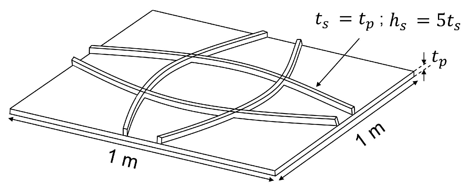
2.3. Stiffener Layout

2.3.1. Stiffener Path

The parametrization presented by [20,21,22] has been modified to characterize the geometry of curvilinear stiffeners. The stiffener curvilinear path is modeled by a cubic spline with 3 control points. The following assumptions have been made to reduce the number of design variables of the stiffener layout. Four symmetrical stiffeners are attached to the skin. Thus, it is sufficient to define the geometry of one stiffener. The start point of the stiffener, A, is located at the bottom edge of the plate. The end point, B, is placed at the plate upper edge on the same vertical as the start point.

Consequently, the stiffener layout is governed by two design variables: $\epsilon$ and $\alpha$. The $\epsilon$ parameter is defined on the plate boundary and varies from 0 to 1, where 1 is the whole perimeter and controls the stiffener location. The $\alpha$ parameter is the normalized distance to the midpoint C and controls the stiffener shape. This approach allows a reduced number of design variables and facilitates to control that the stiffeners lie inside the panel. Figure 6 illustrates the curvilinear stiffener layout that is considered in this work.

The stiffener could also be modeled directly by the coordinates of the points, resulting in four design variables. However, the geometry parameterization chosen here, in its most general form, requires three design variables (${\epsilon }_A,{\epsilon }_B,\alpha$).

The geometry parameterization is simplified in the case of straight stiffener design. For a straight stiffener, the star point A and the end point B are the only control points. Therefore, no curvature parameter is required and the $\epsilon$ parameter defines the stiffener layout.

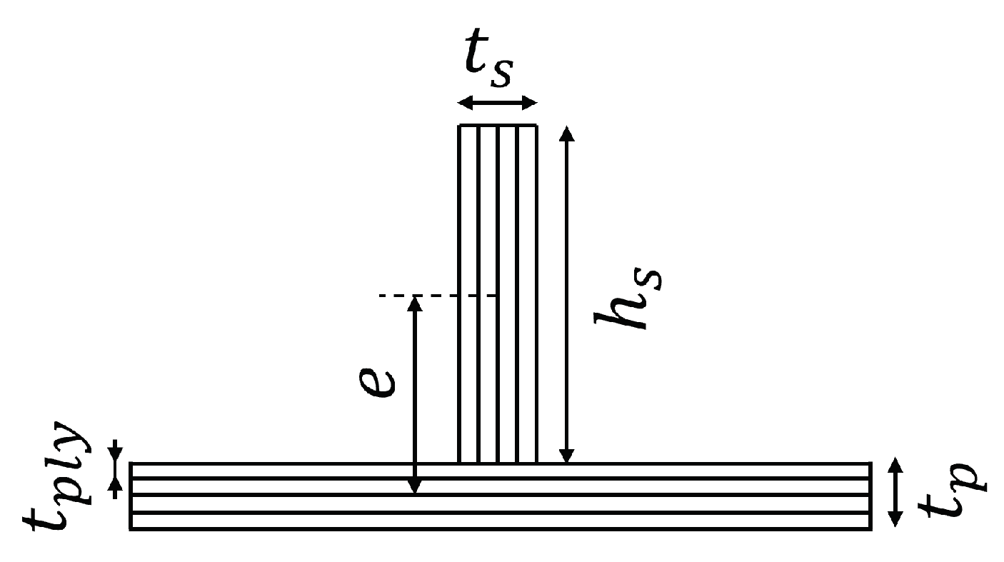
2.3.2. Stiffener Cross Section

Once the stiffener path is parameterized, its cross section is defined. The AFP machine successively places one tow on top of another to manufacture the stiffeners. This results in a rectangular stiffener cross-section, described by two dimensions: the stiffener thickness, $t_s$, and the stiffener height, $h_s$. The stiffeners are modeled by 2-node linear beam element (B31, Timoshenko beam).

The stiffener laminate is assumed to be perpendicular to the plate midplane. In addition, the strong direction of the material is set to be coincident with the longitudinal direction of the stiffener. This simulates that the fibers are aligned with the local orientation of the stiffeners, i.e, the fibers follow the stiffener path, as it can be seen in Figure 6 for curvilinear stiffeners. Thus, the stiffeners are modeled with a zero angle laminate. The zero angle fiber ply in the stiffener is shown to provide a larger bending stiffness to the plate, enhancing the structural stability of the design [20].

The stiffeners are attached eccentrically to the plate. The stiffener eccentricity is defined in Equation (10) as the offset between the stiffener centroid and the panel midplane [20].

$$e=\frac{1}{2}\left(h_s+t_p\right)$$

(10)

Figure 7 indicates the dimensions of cross-sectional view of the panel.

Abaqus’ built-in tie constraint has been used to attach the stiffeners to the plate. The tie constraint ties two separate surfaces together so that there is no relative motion between them [25]. Its major advantage is that it allows fusing together a pair of regions with dissimilar meshes, as it is the case here. Therefore, it is not necessary for the stiffener nodes to coincide with the plate nodes, which reduces the complexity of the setup.

Zhao et al. [27] studied the buckling behaviour of a curvilinearly grid-stiffened panel. This work has been employed to validate the Python script developed to model curvilinear stiffeners. The error between the buckling load reported by Zhao et al. and that obtained by the present model was less than 2%.

3. Optimization Statement

Genetic Algorithm (GA) is employed as the optimizer in this work. The optimization process has been implemented in MATLAB. The objective of the optimization is to maximize the buckling load of grid-stiffened composite panels. To this end, the objective function, f, to be minimized is the inverse of the normalized buckling factor, $\overline{BF}$. The buckling factor is defined as the ratio of the buckling load and the applied load. The buckling factor is normalized to the buckling factor of the first evaluation of the objective function.

The design variables, $\mathbf{x}$, when optimizing straight fiber panels are as follows. One fiber angle per different ply in the skin laminate, $T^i$. Two different plies for the skin laminate are considered, resulting in two design variables: $T^1$ and $T^2$. The stiffener location $\epsilon$ is the other design variable. The optimization of straight fiber panels is unconstrained since the maximum curvature allowed by the AFP machines does not affect it. The straight fiber optimization problem can be defined as:

$$\begin{array}{cc}\hfill \mathrm{Minimize}& f=\frac{1}{\overline{BF}}\hfill \\ \hfill \mathrm{w}.\mathrm{r}.\mathrm{t}.& \mathbf{x}=\left[T^i,\epsilon \right]\hfill \end{array}$$

(11)

The design variables, $\mathbf{x}$, for the curvilinear fiber optimization are defined for the skin laminate and for the stiffener layout. The curvilinear path of the skin fibers is described by two fiber angles (see Equation (1)). The two fiber angles constitute the design variables for each different ply of the laminate: $T_0^i$ and $T_1^i$. The skin laminate is composed of two different plies, so four design variables are required to define it: $T_0^1,T_1^1,T_0^2,T_1^2$. The stiffener layout is determined by the $\epsilon$ location parameter and the $\alpha$ shape parameter, which constitute the other two design variables. Hence, a total of six design variables define the problem, which makes the optimization using GA affordable in computational time. The plate dimensions and the thickness and height of the stiffeners are considered fixed in the optimization.

The curvilinear fiber optimization problem is subject to the manufacturing aspects of the AFP machine. Constraints, g, in terms of the maximum curvature allowable by the AFP machine are imposed for both skin and stiffener fibers. The number of curvature constrains will be equal to the number of different plies of the skin laminate plus the curvature constraint for the stiffener layout. Section 3.1 explains how the curvature of the skin and stiffener fibers is computed.

The optimization formulation for the curvilinear fiber design can be expressed as:

$$\begin{array}{cc}\hfill \mathrm{Minimize}& f=\frac{1}{\overline{BF}}\hfill \\ \hfill \mathrm{w}.\mathrm{r}.\mathrm{t}.& & \mathbf{x}=\left[T_0^i,T_1^i,\epsilon ,\alpha \right],\hfill \\ \hfill \mathrm{subject}\mathrm{to}& & g_i=\frac{\left|{\kappa }_{max,f}^i\right|}{{\kappa }_{AFP}}-1\le 0\mathrm{for}i=1,2,...,m,\hfill \\ & & g_{i+1}=\frac{\left|{\kappa }_{max,s}\right|}{{\kappa }_{AFP}}-1\le 0\hfill \end{array}$$

(12)

where the superscript i denotes the number of different plies within the laminate.

The range of the design variables is indicated in

Table 1. Range of design variables.

	${\mathit{T}}^{\mathit{i}}$	${\mathit{T}}_0^{\mathit{i}}$	${\mathit{T}}_1^{\mathit{i}}$	$\mathit{\epsilon }$	$\mathit{\alpha }$
Lower bound	−1	−1	−1	0	−1
Upper bound	1	1	1	0.25	1

. Note that the fiber angles, $T^i$, $T_0^i$ and $T_1^i$, will be multiplied by 90 and $\epsilon$ and $\alpha$ will be converted to x,y coordinates when the FE model is built.

In the present work, the following values of GA parameters have been chosen based on the authors’ experience as a compromise between the sufficient reliability of the optimal solution and a reasonable calculation price. A population size of ten times the number of design variables. The stopping criterion has been set at maximum of 60 generations.

3.1. Curvature Constraint

The design of composite panels with curvilinear fibers and curvilinear stiffeners should consider the limit allowed on the maximum curvature by the AFP machine. This manufacturing constraint is imposed to avoid local wrinkling when the tow is overly curved. According to A. Blom [28], the curvature for the tow configuration chosen (course of 32 tows with a width of $3.175\times {10}^{-3}$ $\mathrm{m}$) is limited to $k_{AFP}=1.57{\mathrm{m}}^{-1}$.

The fiber path of the skin and stiffeners is 2D, therefore, the curvature definition for a planar function (Equation (13)) is employed.

$$\kappa =\frac{y^{″}}{{(1+{\left(y^{\prime }\right)}^2)}^{3/2}}$$

(13)

Here below, it is explained how to compute the curvature, first for the skin fibers and then for the stiffener fibers.

3.1.1. Skin Fibers Curvature Constraint

In the shifted method, the fiber paths have identical orientation. The fiber path defined by the linear variation of the angle is antisymmetric. This means that is only necessary to compute the curvature for the positive side of the reference fiber path.

The curvature of the skin fibers can be calculated by Equation (13), in which $y\left(x\right)$ stands for the fiber reference path. After a little algebra, the curvature is obtained in terms of $T_1$, $T_0$, $\theta \left(x\right)$ and a, as shown in Equation (14).

$$\kappa \left(x\right)=\frac{T_1-T_0}{a}cos\theta \left(x\right)$$

(14)

The curvature has to be evaluated at x-positions. These x-positions correspond to the center of the (positive) x-divisions of the skin mesh. The maximum curvature of the fiber path, ${\kappa }_{max,f}^i$, is then obtained and compared to the maximum curvature of the AFP machine, ${\kappa }_{AFP}$ (see Equation (15)). The absolute value is used since the curvature is a signed quantity.

$$\frac{\left|{\kappa }_{max,f}^i\right|}{{\kappa }_{AFP}}-1\le 0$$

(15)

3.1.2. Stiffener Curvature Constraint

The curvilinear stiffeners are modeled directly in Abaqus using the spline tool. To evaluate the curvature with Equation (13), it is necessary to know the analytical function of the spline. Abaqus calculates the shape of the curve using a cubic spline fit between all points along the spline [25].

The mathematical method to determine the cubic spline function can be found in reference [29] and is not described here for the sake of brevity.

Once the cubic spline function is obtained, it is possible to interpolate the value of an arbitrary point on the stiffener and compute its curvature. Note that the four stiffeners are equal, so the values of the curvature are only calculated for one of them. Next, the relative difference between the maximum curvature of the stiffener, ${\kappa }_{max,s}$, and the maximum curvature allowed by the AFP machine, ${\kappa }_{AFP}$ is calculated and implemented as a constraint (Equation (16)).

$$\frac{{\kappa }_{max,s}}{{\kappa }_{AFP}}-1\le 0$$

(16)

4. Results

4.1. Case Studies

In this study, a square composite panel with dimensions $2a\times 2a$ is optimized. The value of a is set to $0.5$ m. Two laminates are considered for the skin: laminate A composed of 4 plies and laminate B composed of 16 plies. The stacking sequences to be optimized in the case of straight fiber panels are: ${\left[T^1/T^2\right]}_s$ and ${\left[\pm T^1/\pm T^2\right]}_{2s}$. The stacking sequences for the curvilinear skin fibers during the optimization process are: ${\left[〈T_0^1,T_1^1〉/〈T_0^2,T_1^2〉\right]}_s$ and ${[\pm 〈T_0^1,T_1^1〉/\pm 〈T_0^2,T_1^2〉]}_{2s}$. Each ply has a thickness, $t_{ply}$, of $1.27\times {10}^{-4}$ m.

The thickness of the stiffener, $t_s$, is equal to that of the skin, $t_p$, i.e., both laminates have the same number of plies. The stiffener height, $h_s$, is set as five times of the stiffener thickness. Therefore, the stiffener depth ratio, $h_s/t_s$, is 5, a value for which global or plate local buckling modes are expected [20]. The stiffener blade buckling is not considered. Figure 8 schematizes the panel to be optimized and indicates its dimensions.

The parameters to define the tow course, which are the the tow width and the number of tows in a course, are set to $t_w=3.175\times {10}^{-3}m$ and $n_t=32$, respectively.

The material properties of both the skin and the stiffeners are given in

Table 2. Material properties.

Graphite-Epoxi		Epoxi
$E_1$	132.38 GPa
$E_2$	10.76 GPa	$E_m$	3.7 GPa
$E_3$	10.76 GPa
${\nu }_{12}$	0.24
${\nu }_{13}$	0.24	${\nu }_m$	0.3
${\nu }_{23}$	0.49
$G_{12}$	5.65 GPa
$G_{13}$	5.65 GPa	$G_m$	1.4 GPa
$G_{23}$	3.38 GPa

. The properties of a generic epoxy resin, employed to fill the gaps, are also indicated in Table 2. When panels with gaps are optimized, Poisson’s ratios are assumed equal $\left({\nu }_{12}={\nu }_{13}={\nu }_{23}\right)$ because a rule of mixture for ${\nu }_{23}$ has not been stated.

Certain boundary conditions and load cases have been selected to represent what a wing panel of an aircraft may experience. The three different boundary conditions addressed in this work are the following. All plate edges are simply supported and denoted by SSSS. Two plate edges are simply supported at $y=-a,y=a$ and the other two are clamped at $x=-a,x=a$ and denoted by SSCC. All plate edges are clamped and denoted by CCCC.

For the simply supported boundary condition, there is no out-of-plane displacement, i.e., $w=0$. The clamped boundary condition restricts, in addition to the out-of-plane displacement, the rotations along the x-axis and y-axis, i.e., $w={\theta }_x={\theta }_y=0$. In all cases, to avoid body solid rigid motion, the bottom left corner and bottom right corner are constrained to $v=0$ and $u=v=0$, respectively.

The two load cases considered are: biaxial compression load case and biaxial compression plus shear load. Figure 9 schematizes two possible combinations of load cases and boundary conditions.

Hereafter, the optimization results for both straight fiber and curvilinear fiber panels are presented. The optimization of curvilinear fiber panels are performed for ideal laminates, i.e., without gaps, and for laminates with embedded gaps.

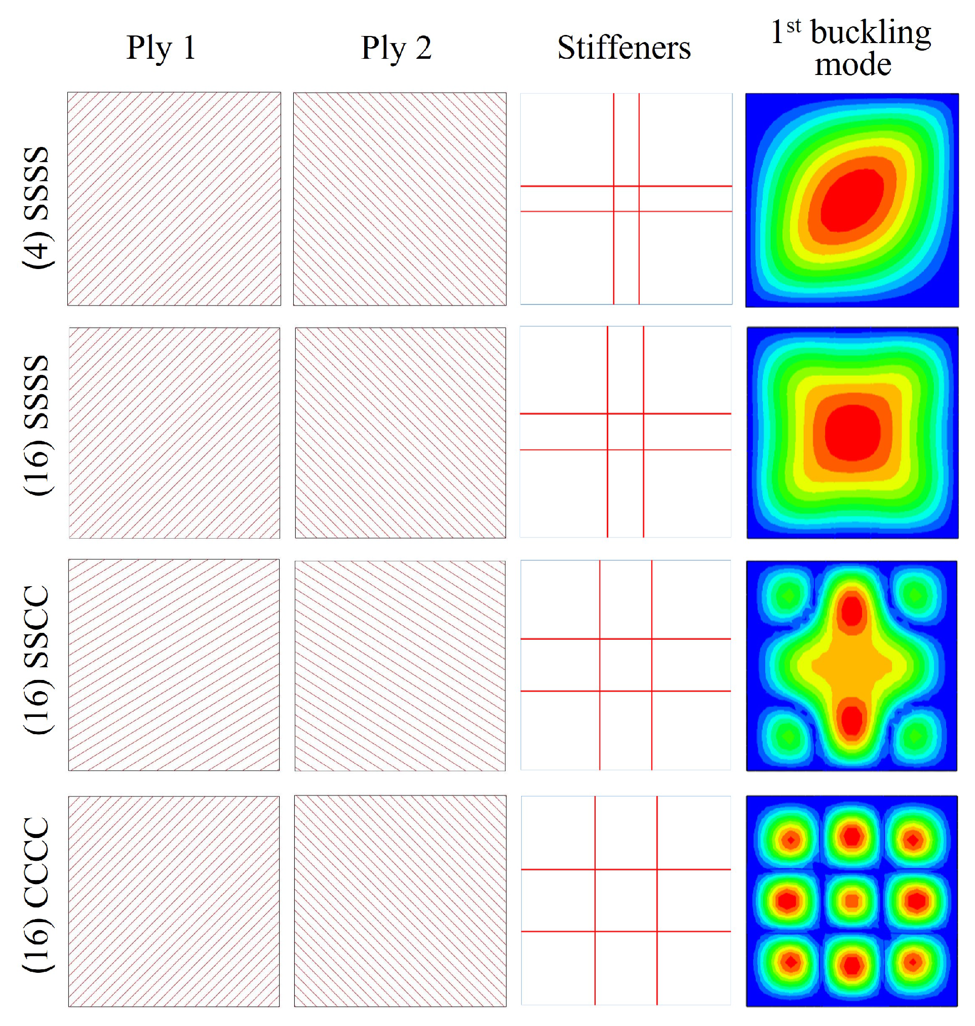
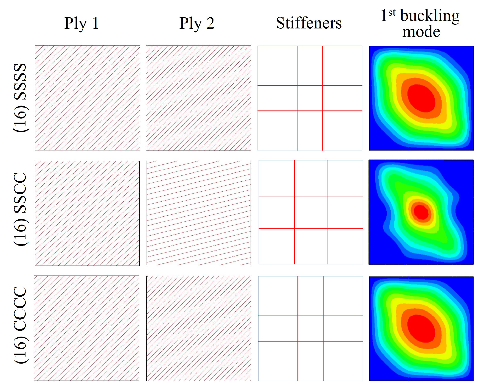
4.2. Straight Fiber Optimization

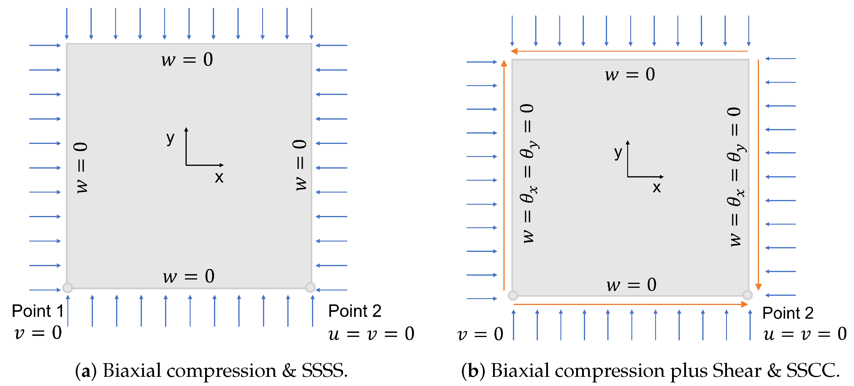
4.2.1. Biaxial Compression Load Case

Four case studies have been optimized for panels subjected to biaxial compressive load: the first one with laminate A (4 plies) and SSSS boundary conditions, the other three with laminate B (16 plies) and boundary conditions of SSSS; SSCC; CCCC.

Table 3. Optimization results of straight fiber panels subjected to a biaxial compression load.

Total Plies	Boundary Conditions	${\mathit{T}}^1\left({}^{\circ }\right)$	${\mathit{T}}^2\left({}^{\circ }\right)$	$\mathit{\epsilon }$	Buckling Load $\left[\mathbf{N}/\mathbf{m}\right]$
4	SSSS	44.9	−45.3	0.140	119
16	SSSS	44.8	−45.1	0.146	20,340
16	SSCC	31.5	−32.5	0.094	43,310
16	CCCC	45.3	−45.5	0.088	48,780

shows the results of the optimization for each boundary condition: the two fiber angles of the stacking sequence (${\theta }_1$, ${\theta }_2$), the stiffener location ($\epsilon$) and the critical buckling load. Figure 10 illustrates the skin layup and stiffener configurations and the first buckling mode shape.

Under SSSS boundary condition, the values of the design variables of laminate A and laminate B are similar. The fiber angles in absolute value are close to 45°. The stiffeners are placed near the center of the panel. The critical buckling loads for laminate A and for laminate B are 119 N/m and 20,340 N/m, respectively. The difference between the two buckling loads is because the number of total plies involves both the laminate thickness and the dimensions of the stiffener blade. The buckling mode is global for both laminates.

For the SSCC boundary condition, the fiber angles in absolute value are approximately 32°. The stiffener positions are biased toward the panel center. The two clamped edges have implied a significant increase in buckling load and a change in the buckling mode shape with respect to the SSSS case. The critical buckling load is 43,310 N/m and the plate buckles locally.

When the CCCC boundary condition is optimized, the fiber angles in absolute value are close to 45° and the stiffeners divide the plate into approximately equal parts. The critical buckling load achieved is 48,870 N/m and the buckling mode is local.

4.2.2. Biaxial Compression Plus Shear Load Case

In this load case, the same boundary conditions have been applied. The laminate A (4 plies) has not been optimized. The results of the optimization are given in

Table 4. Optimization results of straight fiber panels subjected to a biaxial compression plus shear load.

Total Plies	Boundary Conditions	${\mathit{T}}^1\left({}^{\circ }\right)$	${\mathit{T}}^2\left({}^{\circ }\right)$	$\mathit{\epsilon }$	Buckling Load $\left[\mathbf{N}/\mathbf{m}\right]$
16	SSSS	43.9	45.9	0.095	35,380
16	SSCC	42	13.9	0.086	67,650
16	CCCC	48.3	40.1	0.157	85,840

and Figure 11.

For the SSSS boundary condition, the fiber angles have a similar value, approximately 45°. The stiffener locations are towards the panel center. The critical buckling load is 35,380 N/m and the buckling mode is of global nature.

In the case of SSCC boundary condition, there is a significant difference between the values of the fiber angles. The stiffeners are placed such that the plate is split into equal parts. The obtained critical buckling load is 67,650 N/m and the panel buckles globally.

For the last boundary condition (CCCC), the fiber angles differ modestly and the stiffeners are positioned near the panel center. The buckling load obtained is 85,840 N/m and the panel buckles in a global manner.

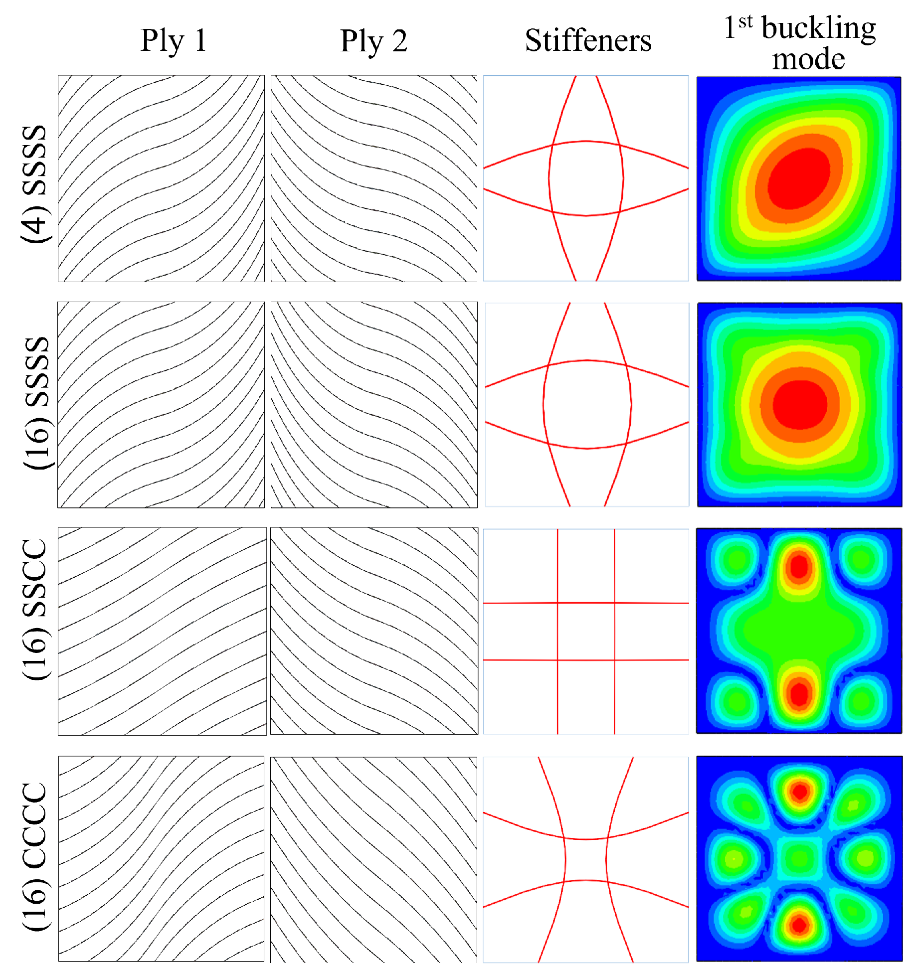
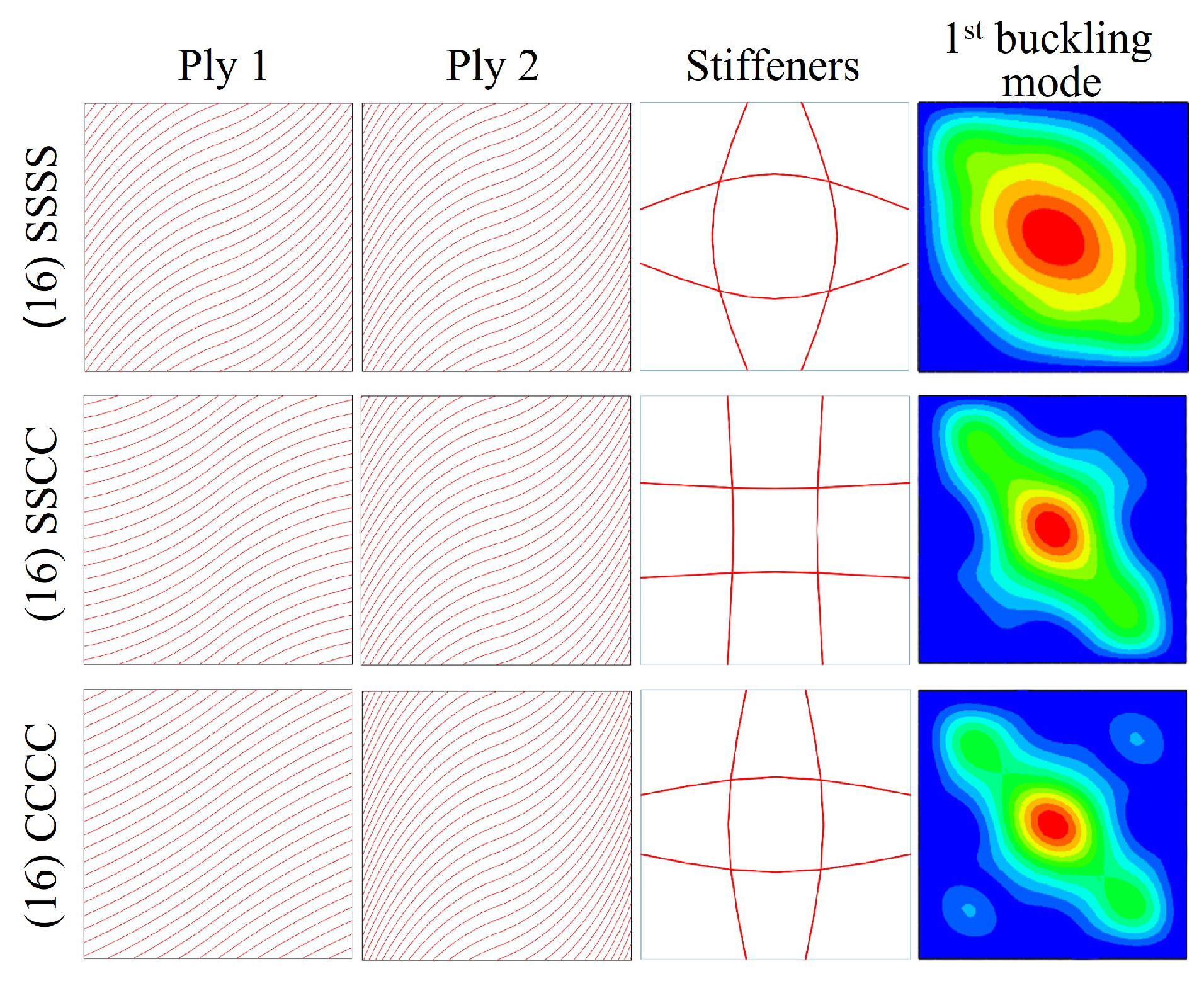
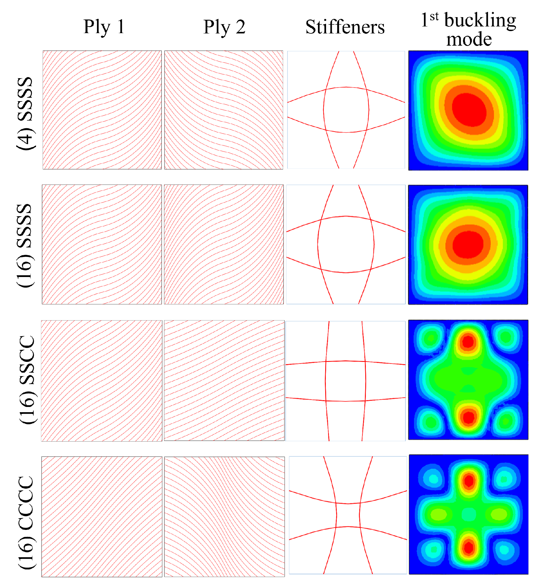
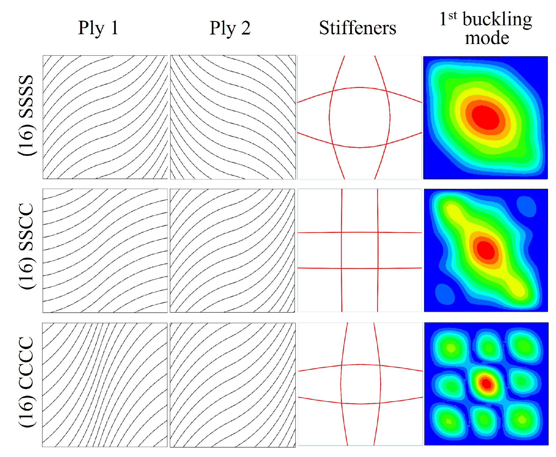
4.3. Curvilinear Fiber Optimization

The same loading and boundary conditions applied to straight fiber panels have been used for the optimization of curvilinear fiber panels. Ideal panels, which here refer to VS laminates without gaps, and panels with embedded gaps have been optimized.

4.3.1. Biaxial Compression Load Case

Table 5. Optimization results of ideal panels subjected to a biaxial compression load.

Total Plies	Boundary Conditions	${\mathit{T}}_0^1\left({}^{\circ }\right)$	${\mathit{T}}_1^1\left({}^{\circ }\right)$	${\mathit{T}}_0^2\left({}^{\circ }\right)$	${\mathit{T}}_1^2\left({}^{\circ }\right)$	$\mathit{\epsilon }$	$\mathit{\alpha }$	Max Curvature $\left[{\mathbf{m}}^{-1}\right]$	Buckling Load $\left[\mathbf{N}/\mathbf{m}\right]$	Improvement $\left(\%\right)$
								${\kappa }_1=1.57$
4	SSSS	14.2	60.9	−11.6	−57.8	0.110	0.387	${\kappa }_2=1.57$	150	25
								${\kappa }_s=1.57$
								${\kappa }_1=1.54$
16	SSSS	13.9	59.5	18.5	66.2	0.0987	0.475	${\kappa }_2=1.57$	24,210	19
								${\kappa }_s=1.57$
								${\kappa }_1=0.876$
16	SSCC	27.5	56	29.3	20.4	0.159	−0.337	${\kappa }_2=0.289$	41,360	−4
								${\kappa }_s=0.377$
								${\kappa }_1=0.305$
16	CCCC	50.2	38.9	−62.1	−21.6	0.177	−0.193	${\kappa }_2=1.30$	49,770	2
								${\kappa }_s=1.32$

indicates the results of the optimization: the value of the design variables, the maximum curvature for ply 1 ($k_1$), ply 2 ($k_2$) and stiffeners ($k_s$), the critical buckling load, and the improvement with respect to the straight fiber design. The configuration for ply 1, ply 2, the stiffener layout, and the first buckling mode for each of the four case studies are shown in Figure 12. The results for panels with gaps are provided in

Table 6. Optimization results of panels considering gap effect, subjected to biaxial compression load.

Total Plies	Boundary Conditions	${\mathit{T}}_0^1\left({}^{\circ }\right)$	${\mathit{T}}_1^1\left({}^{\circ }\right)$	${\mathit{T}}_0^2\left({}^{\circ }\right)$	${\mathit{T}}_1^2\left({}^{\circ }\right)$	$\mathit{\epsilon }$	$\mathit{\alpha }$	Max Curvature $\left[{\mathbf{m}}^{-1}\right]$	Gap Area (%)	Buckling Load $\left[\mathbf{N}/\mathbf{m}\right]$	Improvement (%)
								${\kappa }_1=1.51$
4	SSSS	15.4	60.7	−9	−54.6	0.138	−0.364	${\kappa }_2=1.55$	2.03	145	22
								${\kappa }_s=1.57$
								${\kappa }_1=1.40$
16	SSSS	15.6	57.4	−15.6	−62.2	0.104	0.433	${\kappa }_2=1.55$	2.07	24,190	19
								${\kappa }_2=1.57$
								${\kappa }_1=0.333$
16	SSCC	34	23.6	−20	−50.4	0.160	−0.280	${\kappa }_2=0.990$	1.76	41,010	−5
								${\kappa }_s=0.018$
								${\kappa }_1=1.11$
16	CCCC	55.2	21	−38.8	−56.6	0.183	−0.197	${\kappa }_2=0.481$	1.86	49,360	1
								${\kappa }_s=1.57$

and Figure 13. Table 6 also gives the average gap area encountered for a ply of the laminate. It is calculated as the sum of the gap area in each ply divided by the total laminate area.

A glance at the tables and figures mentioned shows that for the SSSS boundary condition, the fiber angles of ply 1 and ply 2 are comparable in both ideal panels and panels with gaps. The stiffener layout also presents a similarity for both scenarios. The maximum curvatures of the skin and stiffener fibers are near or at the maximum allowable curvature, taking full advantage of the tow steering capability. Although the gaps formed in VS laminates deteriorate the buckling performance, the average gap area for the optimized panels is not much higher than 2%. Therefore, the critical buckling load has not decreased significantly. For panels with embedded gaps, the critical buckling load is 145 N/m if laminate A is optimized, and 24,190 N/m if it is laminate B. The panel buckles in a global manner for all scenarios here. The improvement in the critical buckling load for panels considering gaps with respect to the straight fiber counterparts is 25% for laminate A and 22% for laminate B.

A different behaviour is encountered with the SSCC boundary condition. The skin fibers show considerable curvature, but far from the maximum permitted. The average gap area is 1.76%, which is lower than in cases where the skin fibers reach the maximum curvature. The stiffeners are of very low curvature and similar to the straight fiber configuration. The curvilinear fiber panels have a lower buckling load than the corresponding optimized straight fiber panel. The decrease is greater when the effect of gaps is considered in the VS laminate. For optimized panels with embedded gaps, the critical buckling load has a value of 41,010 N/m and the panel buckles locally with the buckle peaks at the top and bottom edges. In this case, the possibility of the curvilinear fibers has not revealed to increase the panel buckling performance.

In the last boundary condition (CCCC), the fibers of one of the plies do not show a high curvature while the fibers of the other ply are significantly curved. The stiffeners curve significantly towards the center of the panel. The optimum panel considering gaps presents an average percent area of 1.86%. The critical buckling load is 49,360 N/m for the panel with gaps. The panel buckles in a local manner. There is no practical improvement compared to the straight fiber design.

4.3.2. Biaxial Compression Plus Shear Load Case

The results of the optimization for ideal panels subjected to biaxial compression plus in-plane shear are presented in

Table 7. Optimization results of ideal panels subjected to biaxial compression plus shear load.

Total Plies	Boundary Conditions	${\mathit{T}}_0^1\left({}^{\circ }\right)$	${\mathit{T}}_1^1\left({}^{\circ }\right)$	${\mathit{T}}_0^2\left({}^{\circ }\right)$	${\mathit{T}}_1^2\left({}^{\circ }\right)$	$\mathit{\epsilon }$	$\mathit{\alpha }$	Max Curvature $\left[{\mathbf{m}}^{-1}\right]$	Buckling Load $\left[\mathbf{N}/\mathbf{m}\right]$	Improvement $\left(\%\right)$
								${\kappa }_1=1.13$
16	SSSS	20.2	55.0	17.3	63.1	0.100	0.464	${\kappa }_2=1.51$	41,000	16
								${\kappa }_s=1.57$
								${\kappa }_1=0.913$
16	SSCC	37.9	11.2	16.1	63.0	0.169	−0.311	${\kappa }_2=1.57$	69,050	2
								${\kappa }_s=0.249$
								${\kappa }_1=0.390$
16	CCCC	36.2	23.9	20.3	68.7	0.0976	0.353	${\kappa }_2=1.57$	85,620	−0.2
								${\kappa }_s=0.790$

and Figure 14. The results when gaps are considered are given in

Table 8. Optimization results of panels considering gap effect, subjected to biaxial compression plus shear load.

Total Plies	Boundary Conditions	${\mathit{T}}_0^1\left({}^{\circ }\right)$	${\mathit{T}}_1^1\left({}^{\circ }\right)$	${\mathit{T}}_0^2\left({}^{\circ }\right)$	${\mathit{T}}_1^2\left({}^{\circ }\right)$	$\mathit{\epsilon }$	$\mathit{\alpha }$	Max Curvature $\left[{\mathbf{m}}^{-1}\right]$	Gap Area (%)	Buckling Load $\left[\mathbf{N}/\mathbf{m}\right]$	Improvement (%)
								${\kappa }_1=1.50$
16	SSSS	15.9	61	−13.6	−60.2	0.0949	0.488	${\kappa }_2=1.57$	2.08	40,870	15
								${\kappa }_s=1.47$
								${\kappa }_1=1.09$
16	SSCC	42.4	10.4	16.8	62.4	0.161	−0.295	${\kappa }_2=1.51$	1.97	69,010	2
								${\kappa }_s=0.052$
								${\kappa }_1=1.01$
16	CCCC	72.7	36.2	26.3	64.2	0.099	0.322	${\kappa }_2=1.17$	2.26	81,450	−5
								${\kappa }_s=0.665$

and Figure 15.

This load case presents a similar pattern to that of the biaxial compression. For the SSSS boundary case, high values of curvature near or at the limit of the maximum curvature for both plies and stiffener fibers are obtained. The average gap area is 2.08%. The critical buckling load for the panel with gaps is 40,870 N/m and the buckling shape is of global nature. The improvement with respect to the straight fiber counterpart is 16%.

In the case of SSCC boundary condition, the fibers of ply 1 exhibit an important curvature and the fibers of ply 2 are close to the maximum curvature. By contrast, the stiffeners are of very low curvature. The average gap area has a value of 1.97%. For the panel considering the gap effect, the critical buckling load is 69,010 N/m. The improvement over the straight fiber design is 2%. This modest value is mostly due to the skin fiber curvature, as almost straight stiffeners are preferred under SSCC case.

For the CCCC boundary condition case, the skin fibers are considerably curved. The average gap area is 2.26%, which is the highest of all optimized cases. It is because the high value of $T_0$ in ply 1 leads to increased gap formation. The stiffeners show moderate curvature. There is almost no difference between the critical buckling load of ideal VS panel and CS panel. However, the critical buckling load of the VS panel with embedded gaps decreases in a 5% with respect to the CS panel, due to the greater gap formation of the optimized configuration. The value obtained is 81,450 N/m and the buckling mode is local.

5. Conclusions

In this article, a framework has been developed to optimize the buckling performance of composite panels with curvilinear fibers and curvilinear grid stiffeners. The manufacturing aspects of the AFP machine have been considered in the design phase. The maximum curvature allowed by the AFP machine has been imposed on both the skin and stiffener fibers. The effect of the gaps formed when manufacturing VS laminates has been also incorporated. Different load cases and boundary conditions have been studied.

The optimized curvilinear fiber panels presented different configurations depending on the loading and boundary conditions. The curvature of the skin fibers reached in some cases the maximum allowed value and in others it had a moderate value. It was observed that the manufacturing-induced gaps in VS laminates worsened the buckling performance of the panel. Since the optimized panels presented a low gap area, the critical buckling load did not excessively decrease compared to the ideal VS panels. As for the grid layout, the curvilinear stiffeners were generally located in intermediate positions neither near the center nor near the edges of the panel. The stiffeners exhibited a high or even the maximum allowable curvature when SSSS and CCCC boundary conditions were optimized. For the SSCC case, quasi-straight stiffeners were preferred.

It was shown that the difference between the critical buckling loads of optimized curvilinear fiber and straight fiber panels depended on the load case and boundary conditions. The optimized curvilinear fiber panels under the SSSS boundary condition exploited the capability to tailor the stiffness variation to the fullest allowed. The greatest improvement over the straight fiber designs was obtained. By contrast, the optimized VS panels under SSCC or CCCC boundary conditions did not reveal a major advantage with respect to the optimized straight fiber panels. In these cases, straight fiber designs seemed to be preferred. The optimization framework developed could help the designer to evaluate in which scenarios composite panels with curvilinear fibers and grid stiffeners provide the greatest benefit in terms of the critical buckling load.

References

1. Olmedo, R.; Gurdal, Z. Buckling response of laminates with spatially varying fiber orientations. In Proceedings of the Collection of Technical Papers—AIAA/ASME Structures, Structural Dynamics and Materials Conference, La Jolla, CA, USA, 19–22 April 1993; pp. 2261–2269. [Google Scholar] [CrossRef]
2. Almeida, J.; St-Pierre, L.; Wang, Z.; Ribeiro, M.; Amico, S.; Castro, S. Design, modeling, optimization, manufacturing and testing of variable-angle filament-wound cylinders. Compos. Part B Eng. 2021, 225, 109224. [Google Scholar] [CrossRef]
3. Wang, Z.; Almeida, J.; St-Pierre, L.; Wang, Z.; Castro, S. Reliability-based buckling optimization with an accelerated Kriging metamodel for filament-wound variable angle tow composite cylinders. Compos. Struct. 2021, 254, 112821. [Google Scholar] [CrossRef]
4. Castro, S.; Almeida, J.; St-Pierre, L.; Wang, Z. Measuring geometric imperfections of variable-angle filament-wound cylinders with a simple digital image correlation set up. Compos. Struct. 2021, 276, 114497. [Google Scholar] [CrossRef]
5. Almeida, J.; Bittrich, L.; Nomura, T.; Spickenheuer, A. Cross-section optimization of topologically-optimized variable-axial anisotropic composite structures. Compos. Struct. 2019, 225, 111150. [Google Scholar] [CrossRef]
6. Almeida, J.; Bittrich, L.; Jansen, E.; Tita, V.; Spickenheuer, A. Buckling optimization of composite cylinders for axial compression: A design methodology considering a variable-axial fiber layout. Compos. Struct. 2019, 222, 110928. [Google Scholar] [CrossRef]
7. Dang, T.; Kapania, K.; Slemp, W.; Bhatia, M.; Gurav, S. Optimization and postbuckling analysis of curvilinear-stiffened panels under multiple-load cases. J. Aircr. 2010, 47, 1656–1671. [Google Scholar] [CrossRef]
8. Nagendra, S.; Haftka, H.; Gürdal, Z. Design of a blade stiffened composite panel by a genetic algorithm. In Proceedings of the Collection of Technical Papers—AIAA/ASME Structures, Structural Dynamics and Materials Conference, La Jolla, CA, USA, 19–22 April 1993; pp. 2418–2436. [Google Scholar]
9. Hao, P.; C, L.; Yuan, X.; Wang, B.; Li, G.; Zhu, T.; Niu, F. Buckling optimization of variable-stiffness composite panels based on flow field function. Compos. Struct. 2017, 181, 240–255. [Google Scholar] [CrossRef]
10. Sohouli, A.; Yildiz, M.; Suleman, A. Design optimization of thin-walled composite structures based on material and fiber orientation. Compos. Struct. 2017, 176, 1081–1095. [Google Scholar] [CrossRef]
11. Wu, Z.; Weaver, P.; Raju, G.; Kim, B. Buckling analysis and optimisation of variable angle tow composite plates. Thin-Walled Struct. 2012, 60, 163–172. [Google Scholar] [CrossRef] [Green Version]
12. Ijsselmuiden, S. Optimal Design of Variable Stiffness Composite Structures Using Lamination Parameters. Ph.D. Thesis, Delft University of Technology, Delft, The Netherlands, 2011. [Google Scholar]
13. Blom, A.; Lopes, C.; Kromwijk, P.; Gurdal, Z.; Camanho, P.P. A Theoretical Model to Study the Influence of Tow-drop Areas on the Stiffness and Strength of Variable-stiffness Laminates. J. Compos. Mater. 2009, 43, 403–425. [Google Scholar] [CrossRef]
14. Fayazbakhsh, K.; Nik, M.; Pasini, D.; Lessard, L. Defect layer method to capture effect of gaps and overlaps in variable stiffness laminates made by Automated Fiber Placement. Compos. Struct. 2013, 97, 245–251. [Google Scholar] [CrossRef] [Green Version]
15. Brooks, T.; Martins, J. On manufacturing constraints for tow-steered composite design optimization. Compos. Struct. 2018, 204, 548–559. [Google Scholar] [CrossRef]
16. Alhajahmad, A.; Mittelstedt, C. Buckling performance of curvilinearly grid-stiffened tow-placed composite panels considering manufacturing constraints. Compos. Struct. 2021, 260, 113271. [Google Scholar] [CrossRef]
17. Liu, D.; Hao, P.; Zhang, K.; Tian, K.; Wang, B.; Li, G.; Xu, W. On the integrated design of curvilinearly grid-stiffened panel with non-uniform distribution and variable stiffener profile. Mater. Des. 2020, 190, 108556. [Google Scholar] [CrossRef]
18. Wang, D.; Abdalla, M.; Zhang, W. Buckling optimization design of curved stiffeners for grid-stiffened composite structures. Compos. Struct. 2017, 159, 656–666. [Google Scholar] [CrossRef]
19. Praticò, L.; Galos, J.; Cestino, E.; Frulla, G.; Marzocca, P. Experimental and numerical vibration analysis of plates with curvilinear sub-stiffeners. Eng. Struct. 2020, 209, 109956. [Google Scholar] [CrossRef]
20. Zhao, W.; Kapania, R. Buckling analysis of unitized curvilinearly stiffened composite panels. Compos. Struct. 2016, 135, 365–382. [Google Scholar] [CrossRef]
21. Kapania, R.; Li, J.; Kapoor, H. Optimal design of unitized panels with curvilinear stiffeners. In Proceedings of the Collection of Technical Papers—AIAA 5th ATIO and the AIAA 16th Lighter-than-Air Systems Technology Conference and Balloon Systems, Arlington, VA, USA, 26–28 September 2005; Volume 3, pp. 1708–1737. [Google Scholar] [CrossRef]
22. Singh, K.; Kapania, R. Buckling load maximization of curvilinearly stiffened tow-steered laminates. J. Aircr. 2019, 56, 2272–2284. [Google Scholar] [CrossRef]
23. Vescovini, R.; Oliveri, V.; Pizzi, D.; Dozio, L.; Weaver, P. Pre-buckling and Buckling Analysis of Variable-Stiffness, Curvilinearly Stiffened Panels. Aerotec. Missili Spaz. 2020, 99, 43–52. [Google Scholar] [CrossRef]
24. Tatting, B.; Gürdal, Z. Design and Manufacture Tow Placed Plates of Elastically Tailored; NASA/CR: Silicon Valley, CA, USA, 2002.
25. Dassault Systemes. Abaqus 6.14 Documentation. 2014. Available online: http://130.149.89.49:2080/v6.14/ (accessed on 10 December 2021).
26. Waldhart, C. Analysis of Tow-Placed, Variable-Stiffness Laminates. Master’s Thesis, Faculty of the Virginia Polytechnic Institute and State University, Arlington, VA, USA, 1996. [Google Scholar]
27. Zhao, W.; Kapania, R. Vibration analysis of curvilinearly stiffened composite panel subjected to in-plane loads. AIAA J. 2017, 55, 981–997. [Google Scholar] [CrossRef]
28. Blom, A.W. Structural performance of fiber-placed, variable-stiffness composite conical and cylindrical shells. Ph.D. Thesis, Delft University of Technology, Delft, The Netherlands, 2010. [Google Scholar]
29. Kiusalass, J. Numerical Methods in Engineering with MATLAB; Cambridge University Press: Cambridge, UK, 2010; Chapter 3. [Google Scholar]
Figure 1. Reference path defined by the the linear variation of the fiber angle.
Jcs 05 00324 g001
Figure 2. Modelling of tow steered 20 , 50 ply.
Jcs 05 00324 g002
Figure 3. Intersection between the shifted course and the reference course.
Jcs 05 00324 g003
Figure 4. Intersection between the mesh of the skin and the gap distribution.
Jcs 05 00324 g004
Figure 5. Scaled material properties according to gap area fraction.
Jcs 05 00324 g005
Figure 6. Stiffener layout.
Jcs 05 00324 g006
Figure 7. Cross-section of the panel.
Jcs 05 00324 g007
Figure 8. Scheme of the panel to be optimized.
Jcs 05 00324 g008
Figure 9. Two combinations of load cases and boundary conditions.
Jcs 05 00324 g009
Figure 10. Optimized straight fiber panels subjected to biaxial compression.
Jcs 05 00324 g010
Figure 11. Optimized straight fiber panels subjected to biaxial compression plus shear.
Jcs 05 00324 g011
Figure 12. Optimized ideal panels subjected to biaxial compression.
Jcs 05 00324 g012
Figure 13. Optimized panels considering gap effect, subjected to biaxial compression.
Jcs 05 00324 g013
Figure 14. Optimized ideal panels subjected to biaxial compression plus shear.
Jcs 05 00324 g014
Figure 15. Optimized panels considering gap effect, subjected to biaxial compression plus shear.
Jcs 05 00324 g015