Abstract
The behavior of fiber suspensions during flow is of fundamental importance to the process simulation of discontinuous fiber reinforced plastics. However, the direct simulation of flexible fibers and fluid poses a challenging two-way coupled fluid-structure interaction problem. Smoothed Particle Hydrodynamics (SPH) offers a natural way to treat such interactions. Hence, this work utilizes SPH and a bead chain model to compute a shear flow of fiber suspensions. The introduction of a novel viscous surface traction term is key to achieve full agreement with Jeffery’s equation. Careful modelling of contact interactions between fibers is introduced to model suspensions in the non-dilute regime. Finally, parameters of the Reduced-Strain Closure (RSC) orientation model are identified using ensemble averages of multiple SPH simulations implemented in PySPH and show good agreement with literature data.
1. Introduction
Molding of discontinuous reinforced polymer fiber suspensions, e.g., glass fibers in polymer melt, leads to fiber reorientation. Understanding and predicting the behavior of such fiber suspensions is crucial for achieving high quality products in common composite manufacturing processes such as injection molding and compression molding. Due to the high cost of production facilities and molds, it is desirable to simulate the flow in a computationally efficient and reliable way before running experiments. The fiber reorientation is also of high interest for subsequent anisotropic structural simulations in the framework of a continuous CAE chain [1,2].
Jeffery [3] was the first to analytically derive the motion of a single rigid, ellipsoidal shaped body in a viscous Newtonian flow without buoyancy or inertia. Jeffery’s work was extended by Folgar and Tucker [4] to account for fiber interactions by introducing a fiber interaction coefficient that models isotropic diffusivity of fiber orientation. Other phenomenological parameters were introduced to capture experimentally observed orientation delays in the SRF and RSC model [5] and to account for anisotropic diffusion in the Anisotropic Rotary Diffusion (ARD) model [6] or the improved Anisotropic Rotary Diffusion (iARD) model [7]. These phenomenological parameters account for interactions of multiple fibers in non-dilute suspensions and are fitted to experimental observations, but do not describe a two-phase suspension. Instead, they model the fiber orientation state with second and fourth order moments of the fiber orientation distribution function introduced by Advani and Tucker [8] as fiber orientation tensors
and
Here, describes a fiber direction and is the surface element on a unit sphere . Typically, a closure approach for the fourth order fiber orientation tensor is employed to describe the evolution of the second order fiber orientation tensor. Whenever this work utilizes a closure approximation, the invariant-based optimal fitting (IBOF) closure is chosen [9]. Determining the parameters in these macroscopic models from experiments can be time consuming. Thus, a direct fiber simulation may be utilized to identify these parameters.
1.1. Point-Wise Interaction Methods
A common approach for the simulation of fiber suspensions is the treatment of fibers as slender bodies that interact with the fluid at discrete points. Exact solutions from Stokesian dynamics [10] or slender-body theory [11] are utilized to describe long-range hydrodynamic interaction between fluid and particles for creeping flows. Several authors proposed models for single flexible fibers suspended in a fluid. Hinch [12] started by modeling inextensible threads. Yamamoto et al. [13,14] developed a fiber model consisting of individual beads that experience Stokesian drag forces from the fluid. These bead chain models are computationally expensive and authors have combined multiple beads to rods leading to more efficient rod chains [15,16,17]. Alternatively, spheres [18,19] and spheroids [20] connected with hinges were suggested. Lindström and Uesaka [21] use a discrete field of point forces to ensure that the fluid is experiencing forces opposed to the fiber (two-way coupling). Several authors investigated rheological properties of multiple rigid fibers suspended in a fluid based on these models for single fibers. Yamane et al. [22] described the motion of multiple rigid rods with hydrodynamic drag force and torque on the individual rods. They added a lubrication force for rods that are in close proximity to each other in order to capture short range hydrodynamic effects. However, they did not account for long range hydrodynamic interaction between particles, which was addressed later by Fan et al. [23] using slender-body theory. Sundararajakumar and Koch [24] showed that lubrication forces alone do not prevent penetration of fibers and included contact forces. Suspensions of multiple flexible fibers were investigated with rod-chain models [25] and simplified bead chain models [26]. In addition to these rheological investigations, few direct simulations have been applied on component scale with flexible fibers or bundles to investigate effects such as fiber-matrix separation [27,28,29,30].
1.2. Resolved Methods
In contrast to models based on discrete point-wise interaction forces, the suspension flow might be also described directly by a two-phase flow, in which one phase represents fibers and the other one the suspending fluid. Solving this fully coupled two-phase system with mesh-based approaches such as Finite Elements or Finite Volumes raises the problem of large mesh deformations. A simulation using an immersed boundary method resolves the remeshing problem but requires a mesh resolution significantly smaller than the fiber diameter to track the interface and is therefore computationally expensive. An alternative approach for the simulation of two-phase fiber suspensions is the use of particle methods. Meshless particle methods can offer a natural way to represent fluid-structure interaction at the fiber surface and have been studied less than point-wise interaction methods. Bian and Ellero propose a splitting scheme for separate integration of long-range hydrodynamic interactions and short-range lubrication [31], which was applied in an SPH simulation of a concentrated spherical particle suspension [32]. The fine resolution of suspended particles leads to a high accuracy, but comes at high computational costs. Yashiro et al. [33,34] connected particles to rigid bodies for modeling the injection molding of dilute short-fiber-reinforced composites using a moving particle semi-implicit method. Recently, a very similar approach using SPH was reported by He et al. [35,36]. However, both showed only short time periods when comparing the simulation to Jeffery’s equation and did not investigate the interaction between fibers. Fiber suspensions were also investigated in the framework of dissipative particle dynamics with a focus on Boger fluids [37]. This investigation used a Langrange multiplier to constrain fiber extension and multiple parameters had to be calibrated to analytical solutions in order to achieve correct hydrodynamic forces on the fiber. Yang et al. [38] employed the SPH method in order to simulate a single flexible fiber in a viscous fluid with a focus on determining its drag coefficient. However, they limited their work to a single fiber without interactions.
The present work extends Yang’s model with a viscous surface traction term necessary to meet Jeffery’s equation precisely and allows for the simulation of non-dilute fiber suspensions through the introduction of fiber contact forces. First, rotation and bending of a single fiber is compared to Jeffery’s equation to validate the approach. Then, parameters of the RSC fiber orientation model are determined using SPH simulations.
2. Theory
SPH was developed independently by Lucy [39] and Gingold & Monaghan [40] for astrophysical problems in 1977. Since then, multiple formulations were developed and were applied to various fields. The core idea of SPH is the conversion of a partial differential equation (PDE) for a continuum into a set of ordinary differential equations (ODE) for multiple Lagrangian particles. The ODEs are then integrated for each particle to determine their properties (such as mass density or velocity) and position for the next time step. Since particles carry the mass and are moved according to the velocity field, this method conserves mass exactly and treats pure advection correctly. Any arbitrary property in an n-dimensional domain at a position can be described using an integral of the form
employing the Dirac distribution . The two fundamental approximations of SPH are the description of the continuous integral over the domain using a sum over interpolation points, that can be interpreted as particles, and the replacement of the Dirac distribution with a smooth kernel . Here, h describes the smoothing length that controls the kernel size and is usually chosen similar to the average initial distance between particles. A very common smooth kernel is the cubic spline kernel defined as
with and a dimension-dependent normalization factor . Employing the kernel , Equation (3) can be approximated as
denoting a particle’s property at position as and by expressing the associated volume as ratio between mass and density of the particle. The key is the usage of an analytically differentiable kernel such that
can be computed analytically with the kernel gradient , hence turning the PDE to an ODE. The domain is the set of all particles in the model with subsets for the fluid particles and solid particles consisting of wall particles and fiber particles . There is a wide range of variants and actual implementations for this concept and Monaghan gives a comprehensive review in one of his later publications [41].
The modelling of the fluid phase and its interaction with solid particles follows the work of Adami et al. [42,43]. The basic fiber model is adapted from Yang et al. [38] and extended to account for viscous surface traction as well as fiber interactions.
2.1. Fluid Model
In this work, a Transport Velocity Formulation [43] is used to model the suspending fluid, since it is fairly robust against stability issues such as the tensile instability [44]. Adami et al. [43] separate momentum velocity and advection velocity leading to a Navier-Stokes equation of the form
with density , pressure p, viscosity and body accelerations . The last term is a momentum convection that compensates the deviation between advection velocity and momentum velocity. The difference is based on a virtual background pressure that effectively suppresses tensile instability, but does not influence the actual momentum. Hence, the term is called an artificial stress. The SPH-discretized version of (7) used in this work models the acceleration of particle i in the fluid domain by
with the volume attributed to each particle and the velocity of an adjacent solid , which is explained in the next section. Indices are used to refer to the particle based density , pressure , viscosity , mass , position and velocity . The parameter is a small value to avoid singularities in the formulation. The last term is a momentum convection that compensates the deviation between advection velocity and momentum velocity.
Finally, the discrete conservation of mass is written as
and an equation of state is used to relate mass density to pressure. The equation of state has the form
where describes the nominal density and is a reference pressure chosen large enough to keep the density variation small. The latter is achieved by setting with the speed of sound c set to the tenfold of the maximum speed in the flow, thus limiting density variation to approximately 1%. Following Adami et al. [43], the parameter is set as .
2.2. Interaction between Fluid and Solid Particles
The summation of the first term in Equation (8) includes fiber particles and solid wall particles. Adami et al. [42] determined the pressure of a solid particle from a force balance along the centerline of a solid-fluid particle pair as
with a prescribed acceleration of the solid . The corresponding density may be computed by inverting (10). To ensure a no-slip condition, the velocity of solid particles is modified before insertion in (8) to
where the fluid velocity field is extrapolated and subtracted to ensure zero velocity at the interface between solid particles and fluid particles [42].
In this work, wall particles are represented by three particle layers to ensure full kernel support and move with a constant prescribed velocity
Fibers are represented by a single chain of particles that experience hydrodynamic forces from the fluid, elastic forces from neighbors within the fiber and contact forces from other fibers. The first contribution to acceleration is a hydrodynamic interaction
that balances the momentum together with (8). Modelling the fiber as a single layered chain of SPH particles has also been applied by other authors [38,45], but it has some implications, which are discussed further in Section 2.4. One implication is that the particle spacing is directly related to the fiber diameter by
to ensure that fiber particles and fluid particles describe equal volumes in the beginning of a simulation.
2.3. Basic Model for Flexible Fibers
Besides the description of the fluid phase with SPH, a suitable model for the elastic fiber is needed. Thus, the straight-forward linear elastic bead chain formulation of Yang et al. [38] for tensile forces
and bending moment
can be used as a basis for further model development. Here, E describes Young’s modulus, while A and I are the fiber’s cross sectional area and second moment of area respectively. The vector between two neighboring particles with indices i and j is and the enclosed angle is denoted as . Here, the vector notation of indicates that its direction resembles the axis of rotation. The undeformed reference configuration is denoted with a superscript in both, Equations (16) and (17). The bending moment can be converted to pairs of forces
that act on the particle and its neighbors. Figure 1 illustrates these forces and it can been seen, that generally . It is assumed that torsional torque of the fiber is of minor importance to the orientation evolution investigated in this work. Finally, the acceleration on a particle i due to elastic forces can be summarized as
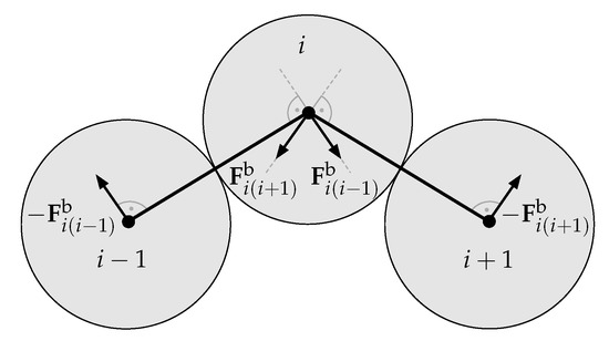
Figure 1.
Force pairs representing bending moment on segments between fiber particles.
If the angle between two adjacent particle pairs exceeds a certain critical value , the neighborhood relation between these particles may be revoked permanently to model fracture of the fiber. Such a criterion is motivated by brittle fiber fracture, as it is typical for glass fibers.
2.4. Viscous Traction at Fiber Surface
A fiber modeled as a particle chain cannot capture a variation of a property in thickness direction of the fiber, as it stores properties at the center line only. Hence, a fiber placed horizontally in a shear flow with periodic boundary conditions, as depicted in Figure 2, would not experience any moment caused by friction forces on its surface. In order to model a physical thickness of the fiber, this work uses an analytical derivation to apply appropriate moment from surface friction to the fiber segment. Figure 3 illustrates a cylindrical fiber segment of length and diameter d with the orientation of its centerline . One exemplary surface normal is shown with its parametrization angle .
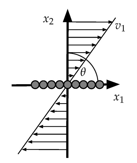
Figure 2.
A fiber is placed horizontally with in a shear flow. The top and bottom walls have a prescribed velocity and a no-slip condition, the boundary conditions in direction are periodical.
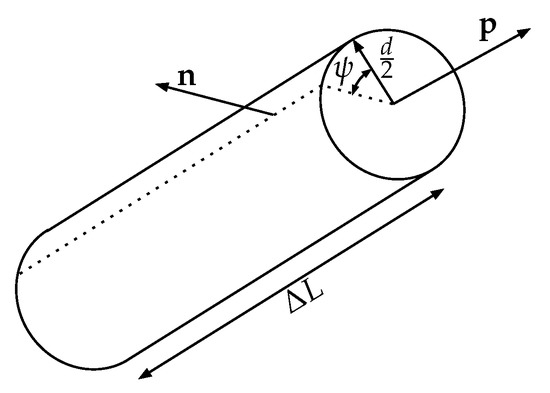
Figure 3.
Cylindrical fiber segment with length , orientation and an arbitrary surface normal .
The fiber direction and any arbitrary surface normal are perpendicular unit-vectors. Any other surface normal can be constructed from this arbitrary normal by rotating it around . The surface normal can be parameterized using and employing a rotational tensor around axis [46]. The parameterized normal becomes
Using this normal, the viscous traction on the surface can be expressed as
if Newtonian viscosity is assumed. This term represents the force acting on each infinitesimal area of the fiber surface. The resulting moment can be computed by integrating with its corresponding leverage as
with a constant fiber diameter d. The term represents an infinitesimal circumferential line segment on the cylinder surface. As the cross product of a vector with itself vanishes, this can be simplified to
The diameter is finite and thus provides some leverage for the traction to generate a moment. The discrete evaluation of (23) is explained in Appendix A. The equation for angular momentum is then multiplied with the distance to its neighbors as a cross product leading to the acceleration of individual particles due to viscous friction
Here, J denotes the moment of inertia for a cylindrical body around its first principle axis of inertia and the factor is chosen to represent the moment by two equal forces at both neighboring particles. This acceleration is then applied to the two neighboring particles and implies hereby a rotational acceleration of a fiber segment, consisting of three particles . The central particle is used to evaluate the velocity gradient of Equation (21) as
It is assumed that the velocity gradient is approximately constant within each segment. In theory, the velocity gradient could be determined at each point of the cylindrical surface from kernel functions, but this comes at much higher computational costs and the difference in the resulting moment is expected to be small.
2.5. Fiber Interactions
If suspended objects come in close contact (10–50% of the radius [26,47]), lubrication forces oppose the relative velocity between fibers. Sundararajakumar and Koch [24] showed that lubrication forces alone do not necessarily prevent penetration at higher fiber volume fractions and added contact forces. The pressure gradient computed from SPH is generally not sufficient to counteract the accumulated forces on the fiber bead chain and does not necessarily prevent penetration of fibers.
It is too simple to apply contact forces directly bead to bead, because this would lead to entangled fibers that interlock at two bead gaps. For the determination of the contact properties at each potential contact pair within the kernel radius, different cases need to be considered:
- Surface-Surface:
- If both interacting particles are located at the center of the fiber (e.g., they have two neighbor particles each, compare Figure 4 at ), the normal direction of contact pair can be computed using the cross productof the involved fiber direction vectors and . The operator is used to conveniently denote the normalization of a vector. Solving the small linear system of equationswith its adjugate matrix leads to the solution for the distance between the fibers and the projections to source and destination vectors and , respectively.
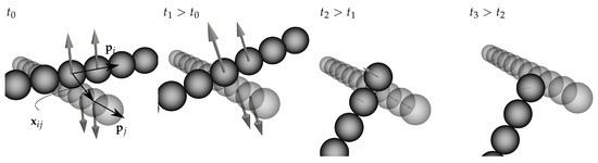 Figure 4. Snapshots of two fibers in contact. At contact initiation , and denote unit vectors for the fiber directions and is the vector between particles of one active contact pair . The contact forces are indicated by arrows which scale with contact force magnitude and rotate in the subsequent time steps ().
 - Surface-End and End-Surface:
- If a particle of a fiber end interacts with a central particle of another fiber, the vector between these two particles can be used to obtain the normal direction by projection. It is assumed that describes a unit vector in fiber direction at one fiber particle at position . Let be the vector from another fibers’ end particle to the point . The closest point to on a line with direction is denoted as and can be used to define the normal direction asUsing the definitions above and the fact that is the projection of to the line with direction , Equation (28) can be rewritten asThe projection on the destination fiber is given as and the contact distance is computed as .
- End-End:
- The simplest case is the interaction of two fiber ends. Here, the vector between those two particles can be simply determined bywith the corresponding distance .
A penalty approach is proposed to prevent fiber penetration, if the distance between fibers falls below the fiber diameter.
The penalty force is formulated as a Hertzian contact force between two cylinders [48]
with
where E is Young’s modulus and denotes the Poisson ratio. Strictly, the contact force varies slightly at fiber ends due to different contact areas. However, the exact pressure distribution in the contact area is not the focus of this work and for high fiber aspect ratios, the portion of fiber end contact becomes relatively small. Thus, the contact force at fiber ends may be rather interpreted as a penetration penalty.
Finally, the particle acceleration due to contact forces is computed as
for each proximity point j with the contact normal and a weighting factor . The weighting factor is necessary to distribute the force at a contact point between particles associated to this contact point and is defined as
with the distance to the previous fiber particle and next particle . Friction in tangential direction is neglected and fiber surfaces are assumed to be smooth. However, friction could be easily incorporated at this point, if the friction coefficient is available. The acceleration is computed for all particles that might possibly contact any other particle and this way, equal force magnitudes on destination and source fibers are ensured.
2.6. Time Integration and Implementation
The time integration is an extension of the kick-drift scheme used in the original transport velocity formulation [43]. The advection velocities are computed for a half step as
based on the previous accelerations at step . Equation (36) utilizes the background pressure to move fluid particles such that no agglomerations or voids form. This is done by modifying the momentum velocity to the advection velocity . The difference in momentum velocity and advection velocity is corrected by the artificial stress in the momentum balance. Fiber particles do not experience a background pressure, as they should not be used to fill voids etc. and thus, their advection velocity is equal to their physical velocity. Then, all particles are moved according to
for the full step. Finally, the velocities are updated as
As this is an explicit time integration scheme, it is only conditionally stable. The maximum time step is computed by
as the minimum of the CFL condition, a viscous condition, a body force condition, a tensile elastic condition and a elastic bending condition. The implementation was realized in PySPH [49] due to its flexibility in implementing the additional equations on top of the transport velocity scheme. The code is publicly available as fork of the original PySPH project (https://github.com/nilsmeyerkit/pysph/tree/fibers).
3. Results
3.1. Rotation and Bending in a Simple Shear Flow
This section presents simulation results for a 3D shear flow (cf. Figure 2) with periodic boundaries in and . The lateral dimensions of the modelled fluid domain are and the dimension in flow direction is with the length of a fiber . The Reynolds number
is set to to be small enough for a quasi-creeping flow, but also as large as possible to increase the time increment. A dimensionless measure for the fiber stiffness is
for a given shear rate G and ellipsoidal aspect ratio [50]. Bending of fibers starts with an increased aspect ratio, higher shear rates and reduced bending stiffness [51]. The dimensionless stiffness S summarises these effects in one parameter.
First, a stiff fiber with is considered. Such a fiber spins in a rigid manner without significant bending and can be compared to the solution of Jeffery’s equation
with vorticity tensor and symmetric strain rate tensor . The shape factor is an alternative measure for the (equivalent) ellipsoidal aspect ratio and is defined as
The solution to Equation (44) is periodic with
being the time for a full rotation of a fiber. When solving Jeffery’s equation for a cylinder with geometric aspect ratio instead of an ellipsoid, Jeffery’s equation can still be applied, but an equivalent aspect ratio has to be used. Such an equivalent aspect ratio was derived by Cox [52] based on slender-body theory and Zhang et al. [53] utilizing Finite Element Analysis. The latter is applicable for small aspect ratios and therefore Zhang’s cubic fit
is used here.
Figure 5 depicts the orientation of a single fiber in shear flow for fiber length and (e.g., the fiber is represented by 5 or 11 particles in a chain). The rotation period obtained with the present SPH approach is sligthly faster than the solution to Jeffery’s equation. One possible reason for the difference is the finite Reynolds number and finite simulation domain with periodic boundaries, whereas Jeffery used an infinite domain with strictly no effect of inertia. Another reason might be the coarse resolution with only one layer of particles for the fiber. Due to the averaging nature of SPH, the exact flow field close to the suspended particles cannot be resolved exactly. The presented approach solves the entire fluid field, but the low resolution and smoothing makes it less accurate than e.g., Stokesian Dynamics simulations. However, the simplicity and computational efficiency make it attractive for engineering applications, such as the parameter fitting presented later.
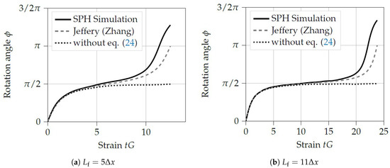
Figure 5.
Orientation angle ϕ for fiber in a shear flow. The fiber length is expressed in multiples of the particle spacing Δx. The dashed gray line represents the solution to Jeffery’s equation with Zhang’s [53] fit. The solid black line represents the solution obtained with this SPH implementation. If the viscous surface traction term (Equation (24)) is neglected, the fiber stops rotating after one half rotation, as shown with the black dotted line.
Bending modes were shown in Yamamoto and Matsuka’s [13] numerical results and the corresponding SPH simulation in Table 1 agree well with their observations. Differences can be attributed to the fact that Yamamoto and Matsuka used an inextensible fiber, while the fibers simulated in this work experience stretching, because the Young’s modulus is taken into account for tensile stiffness as well.

Table 1.
Bending modes of a fiber with length for varied dimensionless stiffness. One example with and critical fiber bending angle is shown to demonstrate fiber fracture.
This section illustrated that the implementation based on SPH can reproduce the rotation periods quantitatively. Furthermore, numerically obtained bending modes can be described qualitatively. In addition, a fully coupled solution for the fluid field is computed. It can be noted that the fluid field obtained for these single fiber setups does not significantly differ from the ideal field. This is reasonable, since a single flexible fiber does not offer much resistance to a highly viscous flow. However, a significant difference can be expected as soon as multiple fibers interact in a concentrated suspension. In that scenario, the presence of suspended fibers and their interactions are expected to raise the macroscopically observed effective viscosity and fiber interactions affect the fiber orientation evolution.
3.2. Parameter Identification for the Orientation Evolution in a Non-Dilute Short Fiber Suspensions
A fully resolved computation of all fibers is often not feasible for full components made from composite material. It can be sufficient to give a reasonable description of the fiber orientation function in terms of a fiber orientation tensor, if these are accurate and scale-separation applies. A common two-parameter model is the RSC model [5] with fiber interaction coefficient and a phenomenological factor that models a delay to compensate an over-prediction in the change of orientation observed in the classical Folgar-Tucker model. In tensor notation, the RSC model reads
with and using the eigenvalues and eigenvectors of the second order fiber orientation tensor . Setting would reduce this model to the Folgar-Tucker model and setting reduces it to Jeffery’s Equation (44). The choice of feasible parameters and remains. Hence, this section computes the orientation evolution in terms of the second order fiber orientation tensor for a small set of fibers in a 3D shear flow and compares the solution obtained with SPH to macroscopic models.
The investigated domain is a cube with edge length and Lees-Edwards boundary conditions [54,55] are employed to induce a shear rate G on the periodic fluid domain. Essentially, these boundary conditions shift dummy particles and particles leaving the domain in -direction according to
with the sign depending on the direction of the shift and the modulo operator . Additionally, the velocity is adjusted
for the shift. Conventional periodic boundary conditions apply in - and -direction, as depicted in Figure 6. All fibers are initially oriented in -direction and randomly positioned in the cube. This unidirectional arrangement is chosen because it can be easily achieved without a micro-structure generator. Instead of analyzing larger representative volumes [26], this work performs multiple realizations of the random process to create a statistical representative behavior. The advantage of this approach is that scatter and standard deviation between random realizations on the micro scale can be observed. The ensemble average of a property is defined as the mean across multiple realizations at the same time step .
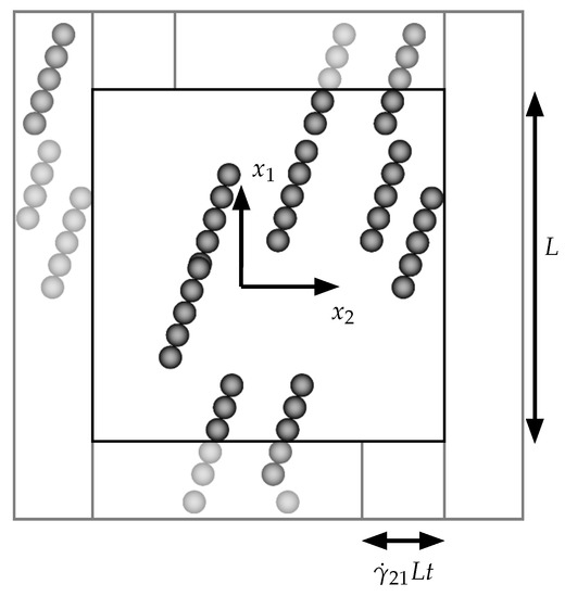
Figure 6.
Setup for the 3D shear with fibers in a cube of edge length . Lees-Edwards boundary conditions [54] are employed to induce a shear rate G. Therefore dummy particles (light gray) and particles leaving the domain in -direction are shifted periodically in during each domain update. Conventional periodic boundary conditions apply to all other sides of the cube. The initial state is generated from fibers aligned in -direction at unique random positions in the entire volume. (Some fibers appear longer in this figure due to other overlapping fibers behind it.)
To obtain optimal parameters at different volume fractions, a least squares fit
is applied to minimize the squared difference of obtained by Equation (48) and the ensemble average of the discrete second order fiber orientation tensor of the SPH analysis. This tensor can be computed as
with each fiber’s orientation . A flexible fiber has different tangential orientations and the tensor’s definition becomes ambiguous then. Consequently, the following examples use fibers with a high stiffness to ensure enough rigidity for an unambiguous interpretation of . However, the method is in no way limited to rigid fibers.
Figure 7 shows the non-trivial components of the ensemble average computed from simulations with five different initial random realizations as a solid green line. The standard deviation at each time step is depicted as light filled area in the background. The gray solid line represents orientation tensor components computed with optimal parameters according to the RSC model given in Equation (48). The simulation time is , which is the time of 10 full rotations of a single rigid fiber. The corresponding strain is approximately 150.
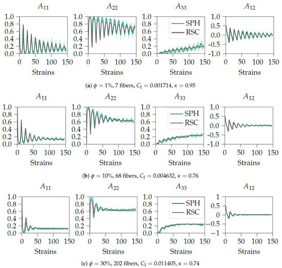
Figure 7.
Ensemble average of fiber orientation tensor components for fibers with aspect ratio rp = 4.43 (Lf = 5) in a 3D shear flow and its comparison to the reduced strain model with optimal parameters. Each simulation result was obtained from five independently sampled initial configurations. The standard deviation is indicated by a light green filled area for each volume fraction.
The simple parameter fitting approach proposed in (51) works well and generally shows a good agreement of macroscopic models with the SPH micro-model. All results show a decreasing orientation amplitude and a trend towards a stationary state with a significant non-zero component in -direction. This trend arises from a combination of fiber contacts and long range pertubations of the flow field that push fibers out of their original trajectories. Figure 8 shows, how fibers are oriented after 30 strains in the case of 10 % fiber volume fraction. Several fibers have left the sheared -plane due to interactions at this point. Eventually, fiber interactions and shear-induced reorientation balance each other and lead to a stationary orientation state. The stationary orientation state is reached faster for increased fiber volume fractions.
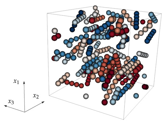
Figure 8.
Snapshot of fibers at 10% fiber volume fraction after 30 strains. The colors are introduced to distinguish fiber particles and represent the particle ID.
The deviations between different initial configurations decrease for increasing fiber volume fraction, as the sample size increases. The deviation between individual realizations at 1% volume fraction is large and it might not be appropriate to describe such a system with a macroscopic fiber orientation model. This highlights that a macroscopic description requires a sufficient scale separation and a sufficient number of fibers to provide reliable results. The proposed SPH simulation can be used to quickly evaluate different configurations and may be used as a tool to not only determine parameters, but also quantify deviations from macromodels, if the underlying conditions of such models are in question for a specific application.
The obtained parameters of the interaction coefficient are compared to Folgar and Tucker’s original work [4] and the values obtained by Phan-Thien et al. [47] in Figure 9. The results from SPH simulations show a good agreement with literature data and support the use of this approach for parameter identification.
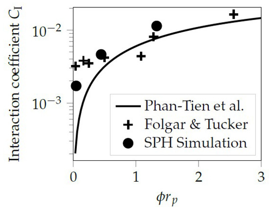
Figure 9.
Comparison of values to the original work of Folgar and Tucker [4] and a fit based on simulation results by Phan-Tien et al. [47]. The values obtained in the presented work are reasonably close to these literature results.
4. Conclusions
Fiber suspensions are treated as flexible bead chains of SPH particles surrounded by other particles representing the fluid domain. The bead chains are connected by elastic tension- and bending forces and interact with the fluid particles in a two-way coupled manner. A novel viscous surface traction term is introduced to compensate the missing fiber thickness that is introduced by the line representation of a fiber. In addition, contact forces are introduced to model fiber interactions in a non-dilute suspension.
The fiber orientation evolution of a single stiff fiber shows good agreement with the rotation periods based on Jeffery’s equation thanks to the introduction of a new surface traction term. Bending modes of single fibers are consistent with results reported in literature.
A periodic domain with Lees-Edwards boundary conditions and suspended fibers is subjected to shear. The investigation of suspensions with different volume fractions of fibers can be used to directly compute the fiber orientation tensor. If several of these computations are evaluated in a statistical sense, the ensemble average can be used to fit optimal parameters of fiber orientation models. For relatively stiff fibers of length , good parameters of the RSC fiber orientation model are found based on the SPH simulation.
In future, the authors plan to extend the investigation to arbitrary initial configurations, flexible and breaking fibers as well as other flow types beyond shear flows. Further, the assessment of standard deviations may enable modeling of uncertainties related to the fiber orientation models.
Author Contributions
N.M.: writing–original draft preparation, methodology, software, visualization; O.S. and M.H.: conceptualization, writing–review and editing; A.N.H.: supervision, conceptualization, writing–review and editing; F.H.: supervision, funding acquisition; L.K.: supervision, methodology, writing–review and editing. All authors have read and agreed to the published version of the manuscript.
Funding
The research documented in this manuscript has been funded by the German Research Foundation (DFG) within the International Research Training Group “Integrated engineering of continuous-discontinuous long fiber-reinforced polymer structures” (GRK 2078). The support by the German Research Foundation (DFG) is gratefully acknowledged.
Acknowledgments
We acknowledge support by the KIT-Publication Fund of the Karlsruhe Institute of Technology.
Conflicts of Interest
The authors declare no conflict of interest. The funders had no role in the design of the study; in the collection, analyses, or interpretation of data; in the writing of the manuscript, or in the decision to publish the results.
Appendix A. Evaluation of the Surface Traction Integral
An arbitrary normal to the fiber direction named must be generated first. This can be achieved by forming the cross product of with an arbitrary other vector that is not parallel to . Chosing the arbitrary vector , the parametrized normal in (20) becomes
The integration in (23) leads to
with the velocity gradient from Equation (25). For the special case that is equivalent to , the moment is computed in the same way with a different arbitrary initial direction, e.g., .
References
- Kärger, L.; Bernath, A.; Fritz, F.; Galkin, S.; Magagnato, D.; Oeckerath, A.; Schön, A.; Henning, F. Development and validation of a CAE chain for unidirectional fibre reinforced composite components. Compos. Struct. 2015, 132, 350–358. [Google Scholar] [CrossRef]
- Görthofer, J.; Meyer, N.; Pallicity, T.D.; Schöttl, L.; Trauth, A.; Schemmann, M.; Hohberg, M.; Pinter, P.; Elsner, P.; Henning, F.; et al. Virtual process chain of sheet molding compound: Development, validation and perspectives. Compos. Part B Eng. 2019, 169, 133–147. [Google Scholar] [CrossRef]
- Jeffery, G.B. The motion of ellipsoidal particles immersed in a viscous fluid. Proc. R. Soc. Lond. Ser. A Contain. Pap. Mathem. Phys. Character 1922, 102, 161–179. [Google Scholar] [CrossRef]
- Folgar, F.; Tucker, C.L. Orientation Behavior of Fibers in Concentrated Suspensions. J. Reinf. Plast. Compos. 1984, 3, 98–119. [Google Scholar] [CrossRef]
- Wang, J.; O’Gara, J.F.; Tucker, C.L. An objective model for slow orientation kinetics in concentrated fiber suspensions: Theory and rheological evidence. J. Rheol. 2008, 52, 1179–1200. [Google Scholar] [CrossRef]
- Phelps, J.H.; Tucker, C.L. An anisotropic rotary diffusion model for fiber orientation in short- and long-fiber thermoplastics. J. Non-Newt. Fluid Mech. 2009, 156, 165–176. [Google Scholar] [CrossRef]
- Tseng, H.C.; Chang, R.Y.; Hsu, C.H. An objective tensor to predict anisotropic fiber orientation in concentrated suspensions. J. Rheol. 2016, 60, 215–224. [Google Scholar] [CrossRef]
- Advani, S.G.; Tucker, C.L. The Use of Tensors to Describe and Predict Fiber Orientation in Short Fiber Composites. J. Rheol. 1987, 31, 751–784. [Google Scholar] [CrossRef]
- Chung, D.H.; Kwon, T.H. Invariant-based optimal fitting closure approximation for the numerical prediction of flow-induced fiber orientation. J. Rheol. 2002, 46, 169–194. [Google Scholar] [CrossRef]
- Brady, J.F.; Bossis, G. Stokesian Dynamics. Ann. Rev. Fluid Mech. 1988, 20, 111–157. [Google Scholar] [CrossRef]
- Batchelor, G.K. Slender-body theory for particles of arbitrary cross-section in Stokes flow. J. Fluid Mech. 1970, 44, 419–440. [Google Scholar] [CrossRef]
- Hinch, E.J. The distortion of a flexible inextensible thread in a shearing flow. J. Fluid Mech. 1976, 74, 317–333. [Google Scholar] [CrossRef]
- Yamamoto, S.; Matsuoka, T. A method for dynamic simulation of rigid and flexible fibers in a flow field. J. Chem. Phys. 1993, 98, 644–650. [Google Scholar] [CrossRef]
- Yamamoto, S.; Matsuoka, T. Viscosity of dilute suspensions of rodlike particles: A numerical simulation method. J. Chem. Phys. 1994, 100, 3317–3324. [Google Scholar] [CrossRef]
- Wang, G.; Yu, W.; Zhou, C. Optimization of the rod chain model to simulate the motions of a long flexible fiber in simple shear flows. Europ. J. Mech. B/Fluid. 2006, 25, 337–347. [Google Scholar] [CrossRef]
- Meirson, G.; Hrymak, A.N. Two-dimensional long-flexible fiber simulation in simple shear flow. Polym. Compos. 2016, 37, 2425–2433. [Google Scholar] [CrossRef]
- Meirson, G.; Hrymak, A.N. Two dimensional long-flexible fiber orientation simulation in squeeze flow. Polym. Compos. 2018, 39, 4656–4665. [Google Scholar] [CrossRef]
- Skjetne, P.; Ross, R.F.; Klingenberg, D.J. Simulation of single fiber dynamics. J. Chem. Phys. 1997, 107, 2108–2121. [Google Scholar] [CrossRef]
- Joung, C.G.; Phan-Thien, N.; Fan, X.J. Direct simulations of flexible fibers. J. Non-Newt. Fluid Mech. 2001, 99, 1–36. [Google Scholar] [CrossRef]
- Ross, R.F.; Klingenberg, D.J. Dynamic simulation of flexible fibers composed of linked rigid bodies. J. Chem. Phys. 1997, 106, 2949–2960. [Google Scholar] [CrossRef]
- Lindström, S.B.; Uesaka, T. Simulation of the motion of flexible fibers in viscous fluid flow. Phys. Fluids 2007, 19, 113307. [Google Scholar] [CrossRef]
- Yamane, Y.; Kaneda, Y.; Dio, M. Numerical simulation of semi-dilute suspensions of rodlike particles in shear flow. J. Non-Newt. Fluid Mech. 1994, 54, 405–421. [Google Scholar] [CrossRef]
- Fan, X.; Phan-Thien, N.; Zheng, R. A direct simulation of fibre suspensions. J. Non-Newt. Fluid Mech. 1998, 74, 113–135. [Google Scholar] [CrossRef]
- Sundararajakumar, R.; Koch, D.L. Structure and properties of sheared fiber suspensions with mechanical contacts. J. Non-Newt. Fluid Mech. 1997, 73, 205–239. [Google Scholar] [CrossRef]
- Schmid, C.F.; Switzer, L.H.; Klingenberg, D.J. Simulations of fiber flocculation: Effects of fiber properties and interfiber friction. J. Rheol. 2000, 44, 781–809. [Google Scholar] [CrossRef]
- Sasayama, T.; Inagaki, M. Simplified bead-chain model for direct fiber simulation in viscous flow. J. Non-Newt. Fluid Mech. 2017, 250, 52–58. [Google Scholar] [CrossRef]
- Londoño-Hurtado, A.; Hernandez-Ortiz, J.P.; Osswald, T. Mechanism of fiber–matrix separation in ribbed compression molded parts. Polym. Compos. 2007, 28, 451–457. [Google Scholar] [CrossRef]
- Ramirez, D. Study of Fiber Motion in Molding Processes by Means of a Mechanistic Model. Ph.D. Thesis, University of Wisconsin Madison, Madison, WI, USA, 2014. [Google Scholar]
- Kuhn, C.; Walter, I.; Täger, O.; Osswald, T. Simulative Prediction of Fiber-Matrix Separation in Rib Filling During Compression Molding Using a Direct Fiber Simulation. J. Compos. Sci. 2017, 2, 2. [Google Scholar] [CrossRef]
- Meyer, N.; Schöttl, L.; Bretz, L.; Hrymak, A.; Kärger, L. Direct Bundle Simulation approach for the compression molding process of Sheet Molding Compound. Compos. Part A Appl. Sci. Manuf. 2020, 132, 105809. [Google Scholar] [CrossRef]
- Bian, X.; Ellero, M. A splitting integration scheme for the SPH simulation of concentrated particle suspensions. Comput. Phys. Commun. 2014, 185, 53–62. [Google Scholar] [CrossRef]
- Vázquez-Quesada, A.; Ellero, M. Rheology and microstructure of non-colloidal suspensions under shear studied with Smoothed Particle Hydrodynamics. J. Non-Newt. Fluid Mech. 2016, 233, 37–47. [Google Scholar] [CrossRef]
- Yashiro, S.; Okabe, T.; Matsushima, K. A Numerical Approach for Injection Molding of Short-Fiber- Reinforced Plastics Using a Particle Method. Adv. Compos. Mater. 2011, 20, 503–517. [Google Scholar] [CrossRef]
- Yashiro, S.; Sasaki, H.; Sakaida, Y. Particle simulation for predicting fiber motion in injection molding of short-fiber-reinforced composites. Compos. Part A Appl. Sci. Manuf. 2012, 43, 1754–1764. [Google Scholar] [CrossRef]
- He, L.; Lu, G.; Chen, D.; Li, W.; Lu, C. Three-dimensional smoothed particle hydrodynamics simulation for injection molding flow of short fiber-reinforced polymer composites. Model. Simul. Mater. Sci. Eng. 2017, 25, 055007. [Google Scholar] [CrossRef]
- He, L.; Lu, G.; Chen, D.; Li, W.; Chen, L.; Yuan, J.; Lu, C. Smoothed particle hydrodynamics simulation for injection molding flow of short fiber-reinforced polymer composites. J. Compos. Mater. 2018, 52, 1531–1539. [Google Scholar] [CrossRef]
- Duong-Hong, D.; Phan-Thien, N.; Yeo, K.S.; Ausias, G. Dissipative particle dynamics simulations for fibre suspensions in newtonian and viscoelastic fluids. Comput. Method. Appl. Mech. Eng. 2010, 199, 1593–1602. [Google Scholar] [CrossRef]
- Yang, X.; Liu, M.; Peng, S. Smoothed particle hydrodynamics and element bending group modeling of flexible fibers interacting with viscous fluids. Phys. Rev. E 2014, 90, 063011. [Google Scholar] [CrossRef] [PubMed]
- Lucy, L.B. A numerical approach to the testing of the fission hypothesis. Astronom. J. 1977, 82, 1013. [Google Scholar] [CrossRef]
- Gingold, R.A.; Monaghan, J.J. Smoothed particle hydrodynamics: Theory and application to non-spherical stars. Mon. Not. R. Astronom. Soc. 1977, 181, 375–389. [Google Scholar] [CrossRef]
- Monaghan, J.J. Smoothed particle hydrodynamics. Rep. Prog. Phys. 2005, 68, 1703–1759. [Google Scholar] [CrossRef]
- Adami, S.; Hu, X.; Adams, N. A generalized wall boundary condition for smoothed particle hydrodynamics. J. Comput. Phys. 2012, 231, 7057–7075. [Google Scholar] [CrossRef]
- Adami, S.; Hu, X.; Adams, N. A transport-velocity formulation for smoothed particle hydrodynamics. J. Comput. Phys. 2013, 241, 292–307. [Google Scholar] [CrossRef]
- Meleán, Y.; Sigalotti, L.D.G.; Hasmy, A. On the SPH tensile instability in forming viscous liquid drops. Comput. Phys. Commun. 2004, 157, 191–200. [Google Scholar] [CrossRef]
- Akinci, N.; Ihmsen, M.; Akinci, G.; Solenthaler, B.; Teschner, M. Versatile rigid-fluid coupling for incompressible SPH. ACM Trans. Graph. 2012, 31, 1–8. [Google Scholar] [CrossRef]
- Cole, I.R. Modelling CPV. Ph.D. Thesis, Loughborough University, Loughborough, UK, 2015. [Google Scholar]
- Phan-Thien, N.; Fan, X.J.; Tanner, R.; Zheng, R. Folgar–Tucker constant for a fibre suspension in a Newtonian fluid. J. Non-Newt. Fluid Mech. 2002, 103, 251–260. [Google Scholar] [CrossRef]
- Johnson, K.L.; Johnson, K.L. Contact Mechanics; Cambridge University Press: Cambridge, UK, 1987. [Google Scholar]
- Ramachandran, P. PySPH: A reproducible and high-performance framework for smoothed particle hydrodynamics. In Proceedings of the 15th Python in Science Conference, Austin, TX, USA, 11–17 July 2016; pp. 127–135. [Google Scholar]
- Baird, D.G.; Collias, D.I. Polymer Processing: Principles and Design; John Wiley & Sons: Hoboken, NJ, USA, 2014. [Google Scholar]
- Forgacs, O.; Mason, S. Particle motions in sheared suspensions. J. Colloid Sci. 1959, 14, 457–472. [Google Scholar] [CrossRef]
- Cox, R.G. The motion of long slender bodies in a viscous fluid. Part 2. Shear flow. J. Fluid Mech. 1971, 45, 625–657. [Google Scholar] [CrossRef]
- Zhang, D.; Smith, D.E.; Jack, D.A.; Montgomery-Smith, S. Numerical Evaluation of Single Fiber Motion for Short-Fiber-Reinforced Composite Materials Processing. J. Manuf. Sci. Eng. 2011, 133, 51002. [Google Scholar] [CrossRef]
- Lees, A.W.; Edwards, S.F. The computer study of transport processes under extreme conditions. J. Phys. C Solid State Phys. 1972, 5, 1921–1928. [Google Scholar] [CrossRef]
- Pan, D.; Hu, J.; Shao, X. Lees–Edwards boundary condition for simulation of polymer suspension with dissipative particle dynamics method. Mol. Simul. 2016, 42, 328–336. [Google Scholar] [CrossRef]


© 2020 by the authors. Licensee MDPI, Basel, Switzerland. This article is an open access article distributed under the terms and conditions of the Creative Commons Attribution (CC BY) license (http://creativecommons.org/licenses/by/4.0/).