Strength Prediction Sensitivity of Foamed Recycled Polymer Composite Structures due to the Localized Variability of the Cell Density Distribution

Abstract

The need for novel methods for the reuse of post-industrial/post-consumer polymer solid wastes (PSW) is of increasing societal importance. Unfortunately, this objective is often limited due to material stream variability or insufficient load-carrying capacity of the fabricated goods. This study investigates a large format fiber-reinforced structural member that contains spatially varying material properties, specifically density. The application is focused on the unique features of closed-cell foamed composite structures made from recycled post-industrial/post-consumer PSW composed of High-Density Polyethylene (HDPE) and Glass Fiber Polypropylene (GFPP). The structures in this research are manufactured using a hybrid extrusion process, which involves foaming enabled by chemical blowing agents that form a fully consolidated solid outer shell and a closed-cell core. The cell distribution is inhomogeneous, in size distribution and spatial distribution, leading to significant spatial variations of the local effective stiffness. To understand the correlation between density variations and effective stiffness and strength, a low-cost method using digital imaging is introduced and integrated into a finite element subroutine. The imaging approach includes sectioning the structural member and analyzing the resulting image using various custom imaging processing techniques in the MATLAB environment. The accuracy of the imaging technique was experimentally verified using a Keyence digital microscope, and the error was found to be 3% in any given spatial feature. The processed image is then correlated to a localized density map of the cross-section using a weighted spatial averaging technique, and the local effective material properties of the foamed region are predicted using the presented micromechanical approach. The local stiffness is a function of void density, local fiber orientation, constitutive behavior of both the fiber and the matrix blend, and the non-linear response of the matrix blend. The spatially varying stiffness and nonlinear strength response at each spatial location are then integrated into a finite element subroutine within the COMSOL multiphysics environment, and results are presented for the deflection and internal stress state of the composite structure. Results indicate that the internal microstructural variations have a nominal impact on the bulk deflection profile. Conversely, results show the peak of the internal stress is increased by ∼11% as compared to the uniform core assumption, thus safe designs must consider core density spatial variations in the final product design.

1. Introduction

Sustainability of polymers has become a significant concern both within the polymer industry and within society, with various researchers focusing on the use of polymer composite structures, specifically plastic lumber, made from various polymer solid wastes (PSW) including Polyethylene and Polypropylene (see e.g., [1,2,3,4]). With the intent of reducing waste and also reducing the use of high density wooden structures, themselves a depleting resource, recycled polymer composite structures are being used as crossties (sleepers), marine pilings, short bridges, and other load bearing applications. Researchers have demonstrated the feasibility of these structures as viable load bearing applications, which are being used all over the world [5,6,7].

The use of fillers, such as glass fibers and natural fibers, are often integrated into the polymer matrix to enhance stiffness, strength, and impact resistance (see e.g., [8,9]). To reduce manufacturing costs, improve light weighting, and allow easy installation of screw fasteners in crossties, chemical blowing agents (CBA) such as azodicarbonamide (ADC) are introduced into the extrusion process [10]. Kord et al. [11] studied the effect of the blowing agent ADC on composites made from High-Density Polyethylene (HDPE), wood flour, and nanoclay. They observed that the increase of ADC content resulted in increased cell size and average cell density, which decreased the overall density of the structure and also reduced the tensile modulus. Therefore, the amount of ADC induced into the composite needs to be precise to achieve an acceptable density spatial distribution to maximize the strength to weight ratio.

When using chemical blowing agents, melt temperature and pressure are key components for nucleation to occur [12]. As PSWs in their molten state are mixed with ADC, the blowing agents undergo a chemical reaction by dissolving into a gas as the pressure in the melt increases. Due to a pressure differential, the nucleation of the individual cells is caused when the gas is released within the mold. The density of the foam varies based on the gas fraction reacted in the molten PSWs, gas lost into the atmosphere, and the rate at which the gas decompresses [12]. As the nucleated cells achieve their maximum growth, the glass fibers in the mold are forced into the dense outer solid shell adding reinforcement to the shell where the maximum stresses are expected [6]. For the expected loading applications, the foamed core does not yield the same stress requirements as the exterior shell. Ruiz et al. [12] observed that when blowing agents are not activated properly, the inactivated ADC particles can form clusters, inducing poor cell morphology and leading to poor internal load transfer.

The cooling rates of the mold have an impact on the formation of cells as well [13]. When the mold is externally cooled using water channels, the shell layer thickness varies based on the total heat transfer between the mold walls and the molten polymer. The molten reinforced polymer is cooled faster in the exterior region limiting the cell growth to the core with a fully densified outer shell. Yousefian et al. [14] studied the Polypropylene/Nano-crystalline cellulose composite and found that by varying mold temperatures between 30 °C and 80 °C, the ratio between the shell and the core could be altered by 5%. Tissandier et al. [15] studied the effects of temperature, blowing agents, and fiber content on composites made from HDPE, flax fiber, and ADC, which were mixed and manufactured using injection molding. This process included applying a temperature gradient (0–60 °C) inside the mold and achieved acceptable microcellular asymmetric structure with high fiber content, blowing agents, and mold temperature. They showed that if a bar is cooled using a gradient, the cell wall thickness on the cooler side is thicker than the warmer side. In their configuration, they concluded that the cold side of the mold controlled the final morphology of the foaming process.

The mold temperature also influences cell size, cell density, and distribution [16]. It was found that as the mold temperature decreases in injection molded HDPE structural foams foamed with ADC, a small but measurable increase is observed in the average cell density and cell size [14]. Cell growth can be limited by increasing the fiber content, which increases the viscosity of the melt and potentially impacting processability [17]. These variations of cell size and its dependence on material properties, namely elastic stiffness, have been studied by Redenbach et al. [18] by using Laguerre tessellations, a weighted mathematical generalization used to model foams using convex cells. They found that as the cell aspect ratio, defined as the ellipsoidal major to a minor axis, increased from spherical, the effective elastic stiffness decreased.

Cell wall thickness also impacts the material properties of foams. Barbier et al. [19] studied Voronoi closed-cell foams (which is a mathematical partitioning of regions in proximity to grid points in space) under a variety of imposed strains caused by wall stretching, and they found a correlation between the density and cell irregularity on the effective elastic and plastic properties. They concluded that under elastic deformation, material properties rely only on relative density. Whereas, under plastic deformation, there is a dependence on both relative density and structural deformation.

To calculate the material properties of closed cell foams, many researchers have used various micromechanical approaches to estimate the effective homogenized medium, specifically, the tensile modulus, as either an isotropic or anisotropic structure (see e.g., [20]). The micromechanical approaches do not account for various combinations of closed cells, including cell sizes, cell shapes, and relative density, to predict the material behavior. Zhang et al. [20] have reviewed various micromechanics models (see e.g., [21,22,23,24,25]) using uniform closed cells by studying HDPE foams made by compression molding techniques. They suggested that the differential scheme [24] and the square power-law suggested by Moore et al. [26] are the most accurate within the cell volume fraction of 0–55%. In the present research, the square-power law will be used. Recently, Lo et al. [27] studied transversely isotropic PVC foams and modeled and predicted the elastic stiffness using unit cell representation for the foam microstructure. They modified the Halpin–Tsai equations by introducing an apparent volume fraction to calculate the material properties and replaced the actual resin volume fraction. Tucker and Liang [28] suggested that the Halpin–Tsai equations are most applicable for long fibers, but for the short fiber the reinforced system employed in the present study, the Tandon and Weng [29] model is more appropriate. The present paper uses the closed form solution of the Tandon and Weng model, implied by Tucker and Liang as derived in the work by Zhang [30], for the fiber reinforced micromechanics modeling.

It has been shown that many structural foams have a spatially varying density gradient that often decreases in density from the outer solid shell to the closed cell foamed core [31]. To understand the complex nature of foams with varying cell sizes, density, and cell size distribution, various studies using images from Scanning Electron Microscopy (SEM) [32], digital microscopy [33,34], and Micro-CT/X-ray [35,36,37] were used. Sadik et al. [33] studied images obtained from a digital microscope at 5× magnification and used the micrographs to binarize cells and measure the void fraction using ImageJ software. The void fraction was then used to calculate linear elastic material properties of the foamed polymer such as tensile, shear, and flexural modulus. These images were analyzed for the foamed structures by using micrographs and calculating the void fractions. Davari et al. [32] studied chemically linked polyethylene foams and the foam morphology using images from SEM. They concluded that density is the dominant parameter for predicting material properties, but when the density is uniform, there is a small but measurable contribution to the material properties as a function of the cell size distribution.

Recently, Zhu et al. [36] used MATLAB image processing techniques to study aluminum foams by examining images obtained from X-ray computed tomography ($\mu$CT) and extended the foam characteristics into a Finite Element Model (FEM). They showed that the image processing techniques can be used to study the porosity of aluminum foams and can reasonably predict the compression behavior. In an attempt to characterize porosity using inexpensive and quick modeling techniques, Yunus et al. [38] studied the porosity of polyurethane foams by using a Canon camera, a black box, and a LaserJet scanner. They then processed the resulting images in a custom MATLAB subroutine. They also validated their results for the porosity measured by each instrument using a stereomicroscope and an SEM. They concluded that the black box results were the most comparable to the results obtained from an SEM.

In a recent work by the authors [39], the composite structures made from recycled materials were studied by integrating the fiber aspect ratio, uniform cell density, orientation state of the fibers, and the constitutive properties of the raw materials. These properties were used as inputs into micromechanics models, and the effective elastic moduli of the solid shell outer core of the composite as well as the foamed core were predicted. Stress values of the raw material were measured at a 0.2% reference strain, and the reference stress of the shell and core formed a nonlinear stress–strain relationship using a modified rule of mixtures and micromechanics models. The predicted elastic moduli and reference stresses were then used in a nonlinear finite element model to predict the flexural deflection response of the composite crosstie under a 4-point bend test using ASTM D6109-13. The results from the model were compared to experimental tests from sixteen different samples, and the finite element results were found to be within the experimental variation.

In this paper, a weighted method is proposed and demonstrated to characterize the density of glass fiber reinforced HDPE/PP (High-Density Polyethylene/Polypropylene) foamed core with cells of varying sizes and distribution using a commercial off-the-shelf (COTS) EOS60D Canon Camera (Canon Inc., Tokyo, Japan). This is achieved by taking 2D images of the cross-section, such as that depicted in Figure 1, using the COTS camera and obtaining a density map by measuring areas of cells contained within the image using image processing techniques implemented in MATLAB (2018a, MathWorks, Natick, MA, USA). The cross-sectional area of the cells within a sample image is tabulated and their results are validated against results obtained using a high-resolution VR-3100 3D digital microscope (Keyence Corporation of America, Itasca, IL, USA). The density map is translated to a point by point mapping of the elastic modulus using a differential scheme. A finite element model is then implemented using a gridding technique to map the spatial varying density results obtained from the imaging results, and the solutions are compared to those from the uniform density method. The von-Mises stress is analyzed for comparison purposes and the results that include local variations in the cell density yield a ~11% higher peak stress as compared to that of the uniform density core. This method will allow for safe design considerations for various applications due to the stresses caused by variations in cell size and distributions.

2. Methodology

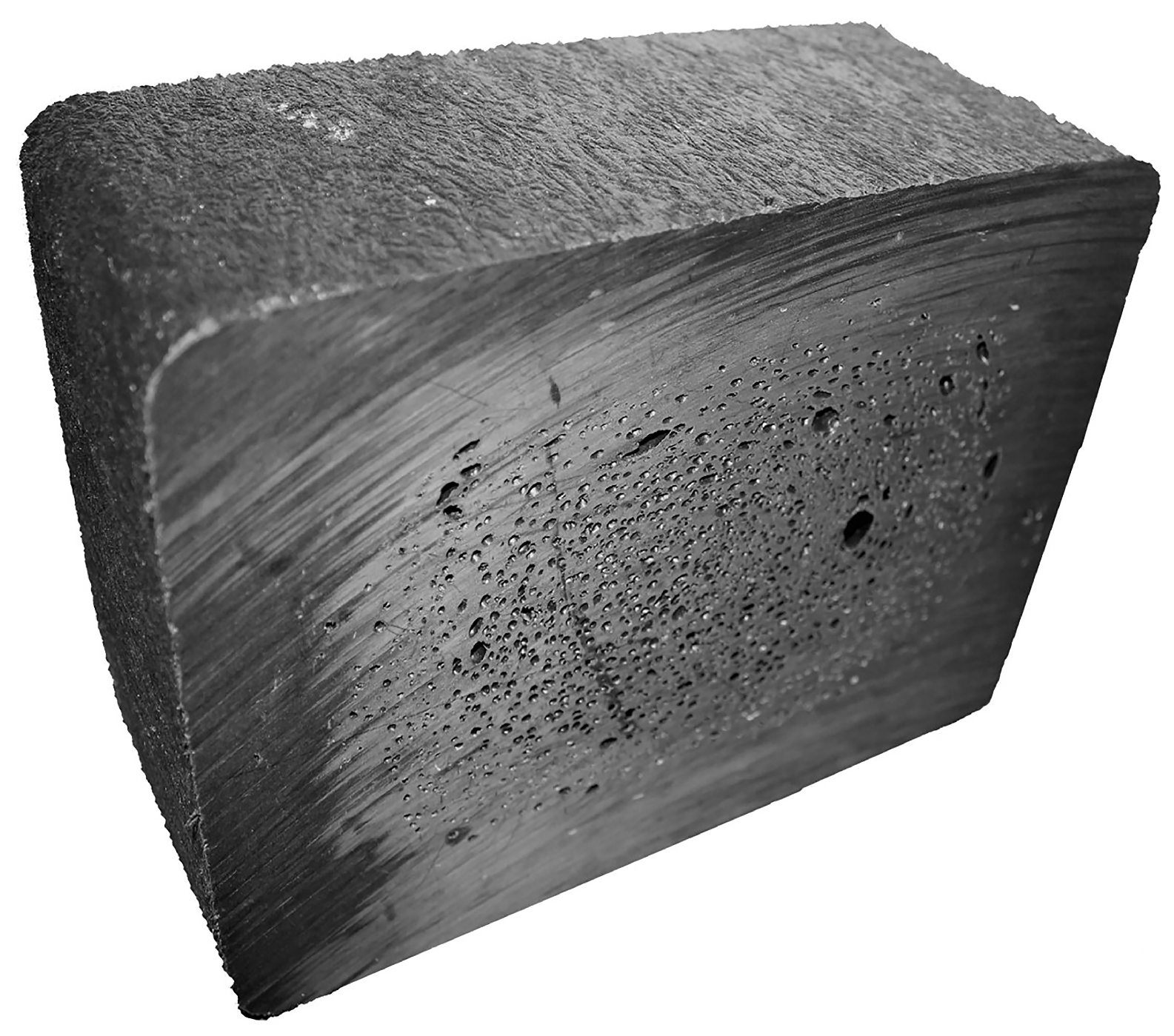
2.1. Materials and Manufacturing

The large-format composite structures discussed in this research are made of a blend of recycled High-Density Polyethylene (HDPE), recycled Glass Fiber Polypropylene (GFPP), ADC (chemical blowing agent), and carbon black. This mixture consists of ~20 % GFPP, ~80% HDPE, ~0.5% ADC, and carbon black by mass. This blend was mixed, melted, and pressurized into a mold cavity. The exterior of the mold was cooled using room temperature water. The cooling affected the outer shell first and allowed the blowing agent to react in the core forming a dense outer core and a foamed inner core, with varying cell size distribution and spatially varying density. Three samples from different crossties were sectioned using an industrial chop saw, and debris from the cutting process was removed. The cross-section of the crosstie was then photographed in a low light environment with the flash from the COTS camera, yielding an image that was approximately 3000 × 2300 pixels. The dimensions of the core for each sample were 0.19 m × 0.14 m (7.38 in × 5.38 in) as shown in Figure 2a.

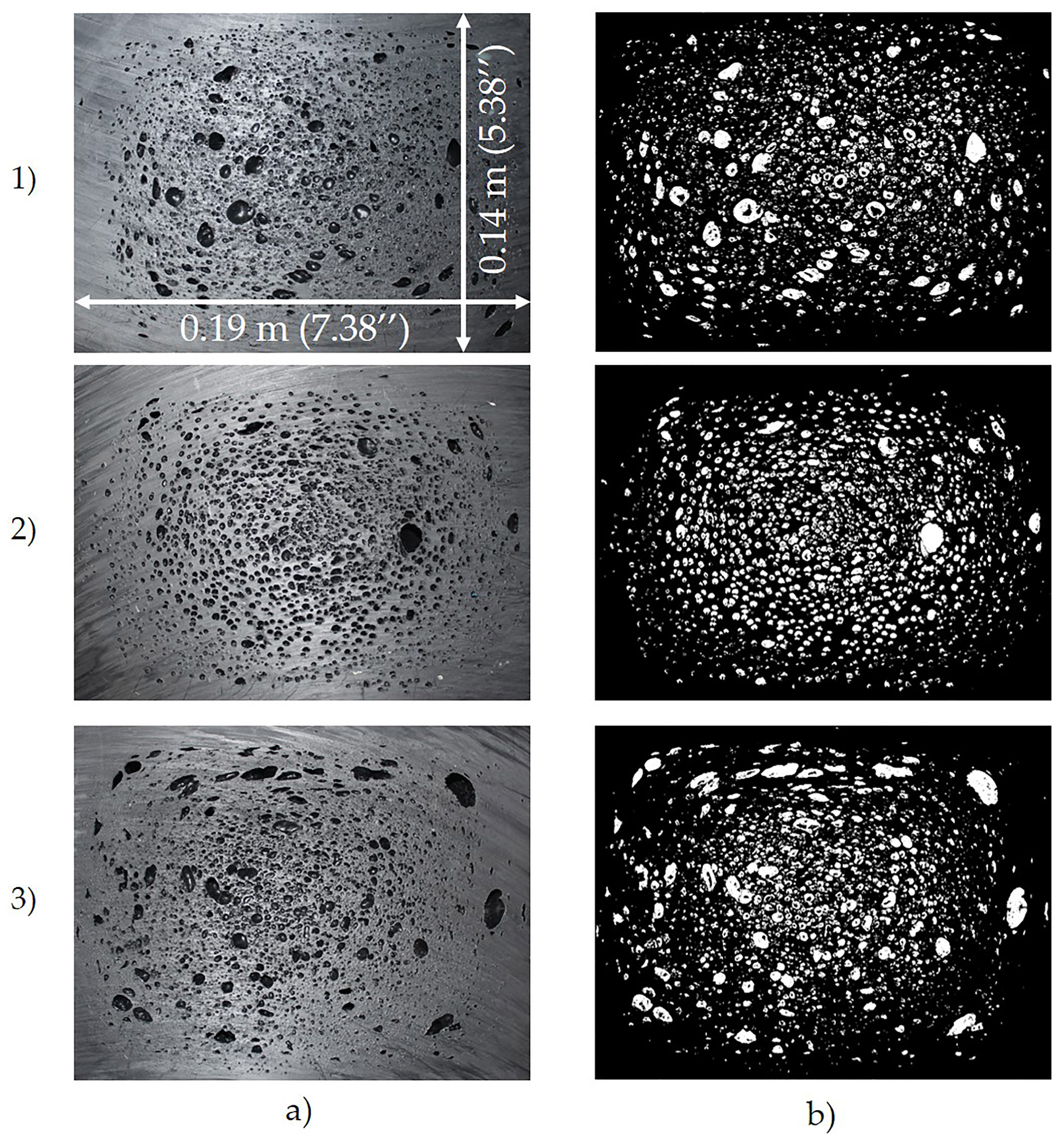
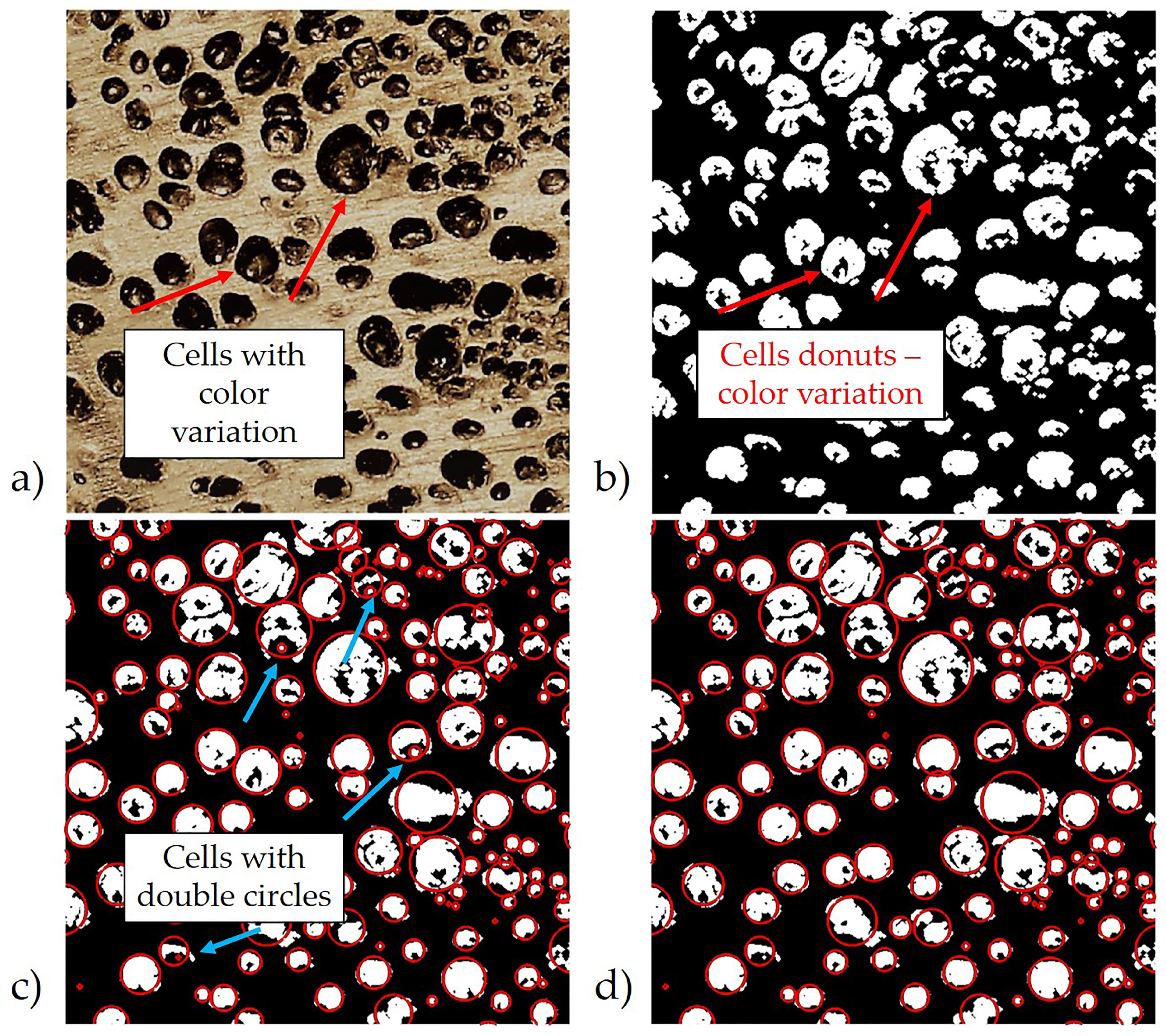
2.2. Image Processing to Generate Cells

The photographed samples were imported into the MATLAB environment as an array representing the image color density as a function of pixel location. The uploaded images taken from three different cross-sections are shown in Figure 2a. Pixels were converted from a grayscale value to a binary value using color contrast differentiation. It was found that a yellow tint using the automatic enhance option included in the Windows photo editor provided reasonable pre-processing contrast variations in differentiating the solid region from the darker cells. A threshold value of 25% was selected for the images, and the noise within the binary image was removed using a morphological structure operation by ignoring individual false single pixels. As shown in Figure 2b, the white pixels denote cells, and the neighboring solid surface region is denoted in black.

This method then considers the effective area of the cells shown in white pixels and draws a circle around it. The dimensions of this circle are defined as the effective diameter using the automated MATLAB subroutine which is much faster compared to highly sophisticated and manual use of an optical microscope. During image processing, false positives must be identified and properly addressed. As seen in Figure 3a,b, it can be noted that in the picture taken with the COTS camera, there are color contrast variations within the cell cavity itself. The first false positive, termed a donut, is a cell region that contains black pixels resembling a solid shell. For the overall sample size of 7.38 × 5.38 inches, the image is approximately 3000 × 2300 pixels, and the size of each pixel is 63.5 $\mathsf{\mu }$m. For the composite structure discussed, the radius of the fibers was measured to be 8.56 $\mathsf{\mu }$m ± 0.57 $\mathsf{\mu }$m [39] and thus the fibers are not visible within the image. Optical microscopy was performed on the surface of the cells, and the fibers did not protrude from the cell wall. A second false positive, termed a double circle, is a shell region that appears to cover a portion of the cell due to flaws introduced from the saw blade used in the sectioning process.

The first false positives were corrected using a subroutine that automatically takes into account the overall area by circles drawn around each cell, including the black pixels within the cell region, as shown in Figure 3c. The second false-positive requires an additional processing step whereby any captured features that reside within the domain of another feature, such as those highlighted in Figure 3c, were removed from consideration. If the double circles were not removed, the area of the cells within the region would be overestimated. Figure 3d shows the cell distribution requiring substantially less archived data as only the centroid and effective radius is stored and used in subsequent processing. This down-select process allows the homogenization algorithm to process more quickly and retains the effective features of the various cells for micromechanical predictions.

It is important to note that the cross-sections shown are cut at a random plane along the longitudinal axis of the composite. As this cutting process may not necessarily pass through the centroid of the cell, it will tend to underestimate the actual cell spherical equivalent volume. To account for the underestimation, a correction factor is used to estimate the largest radius of the 3D spheroidal cell instead of the chord length as seen in a 2D cell. This correction factor is taken from the work of Pinto et al. [40] and the radius of each cell is adjusted as

$$\begin{array}{c}\hfill r_{3D}=1.273r_{2D}\end{array}$$

(1)

2.3. 2D Area Validation

To validate the cell area obtained using image thresholding and the COTS camera, a detailed study was conducted on the subregion of the COTS image shown in Figure 4a for sample 2. This region contains 36 identifiable cells of varying sizes, and each cell is compared to the area measured manually using the high-resolution 3D Keyence 3100 microscope. For example, a single cell was selected and is shown in Figure 4b. Its effective pixel diameter was measured using the image thresholding algorithm discussed above, and the effective area is compared to the area measured using the Keyence digital microscope that includes the non-circular perimeter of the cell in the area calculation. Each of the 36 cells were measured manually using the Keyence digital microscope and their regions are highlighted in Figure 4c. The areas from the aforementioned imaging algorithm, shown in Figure 4d, were then compared to each of manually identified areas from the high-resolution microscopy results.

The total area for the region of one cell is highlighted in Figure 4b. The total area for the cells in the image was calculated with image thresholding approach using the image from the COTS camera as 170.69 mm², and the total area for all 36 cells was measured using high-resolution microscopy was 166 mm², yielding an error of 3%. The error was calculated using the equation,

$$\begin{array}{c}\hfill Err=\frac{|A_{Microscopy}-A_{COTSImaging}|}{A_{Microscopy}}\times 100\end{array}$$

(2)

2.4. Image Mirroring and Density Homogenization

To calculate the homogenized density of the surface for use in the finite element model, a grid of 400 × 250 points was mapped onto the surface of each respective sectioned sample. The sample image was then mirrored about the edges to avoid biasing in any region near the surface and to allow continuous regions for homogenization at all points within the image. A region for a single point was depicted in Figure 5. A fixed pixel radius of $R=300$ was taken for each of the $3000\times 2300$ pixel images, and every cell was identified within the radius R.

The cells identified within the circle were averaged to calculate the local density using an exponential decaying weight function. This allowed the areas of the cells closest to the grid point to have the highest contribution to the effective density, whereas the cells farther from the center have less of a contribution to the effective density. This is also denoted by the color variations, as seen in Figure 5. The cells closest to the center are colored red and provide the highest contribution to the density homogenization, whereas the cells farthest from the center are shown in colors that transition to yellow and then to blue as their contribution decreases. The exponential decay function is defined as,

$$\begin{array}{c}\hfill \tilde{\rho }(x,y)={\int }_0^{2\pi }{\int }_0^{\infty }\psi (r,\theta )e^{-{(r(x,y)/R)}^2}r(x,y)drd\theta \simeq {\int }_0^{2\pi }{\int }_0^{3R}\psi (r,\theta )e^{-{(r(x,y)/R)}^2}r(x,y)drd\theta \end{array}$$

(3)

where r is the local radius from the center of the region of radius R, $\tilde{\rho }(x,y)$ is the localized density, and $\psi (r,\theta )$ is the probability of finding a cell at $r,\theta$. The upper limit on the radial integral is approximated as being upper bounded by $3R$, as this will take into account 99.9% of the area within the distribution while avoiding unnecessary calculations over all cells captured within the image. As observed, the cell sizes are much smaller than the region R. Therefore, for discrete data sets, Equation (3) can be approximated as,

$$\begin{array}{c}\hfill \tilde{\rho }(x,y)\simeq \sum _{i=1}^N{A}_i{e}^{-{(r(x,y)/R)}^2}\end{array}$$

(4)

where $A_i$ is the area of the $i_{th}$ cell and N is the total number of cells in the entire image. Again, Equation (4) as in Equation (3), will disregard cells that have a centroid more than $3R$ from the grid point being analyzed as their contribution will not significantly alter the final solution due to the pre-multiplication of the exponential decaying function. To normalize over the entire area of the image, the density $\rho (x,y)$ is calculated as,

$$\begin{array}{c}\hfill \rho (x,y)=\frac{\tilde{\rho }(x,y){\sum }_{i=1}^N{A}_i}{\int \int \tilde{\rho }(x,y)dxdy}\end{array}$$

(5)

where all the cell areas within the image are summed from i = 1 to N and x and y are the grid points selected.

2.5. Material Properties Prediction

Based on the previous research [39], material properties were predicted using only constitutive properties. This was accomplished using the inputs of raw materials, including as elastic moduli and Poisson’s ratios of HDPE and GFPP, glass fiber aspect ratio, and foamed core density. Since modeling over each individual fiber in a 2.62 m long composite structure is computationally impractical, Advani and Tucker [41] proposed a model which uses the average orientation of the fibers within a region, termed the orientation tensors. Specifically of interest are the second order $a_{ij}$ and the fourth order $a_{ijkl}$ tensors, defined as,

$$\begin{array}{c}\hfill a_{ij}={\int }_{\mathbb{S}}{p}_i{p}_j\psi \left(\mathbf{p}\right)d\mathbb{S},a_{ijkl}={\int }_{\mathbb{S}}{p}_i{p}_j{p}_k{p}_l\psi \left(\mathbf{p}\right)d\mathbb{S}\end{array}$$

(6)

where, $\mathbb{S}$ is the surface of a unit sphere and $\mathbf{p}$ is the unit vector representing an individual fiber. The orientation tensor is symmetric, $a_{ij}=a_{ji}$, and $a_{ijkl}=a_{klij}=a_{jikl}=a_{ilkj}=···$. Based on the property that the integral of the probability density function over the entire unit sphere must be 1, the trace of second-order orientation tensor is similarly equal to 1. For example, the second order orientation tensor of randomly distributed fibers has components of $a_{11}=a_{22}=a_{33}=1/3$ with all other components being equal to zero.

Using the second-order orientation tensor $a_{ij}$, the fourth-order orientation $a_{ijkl}$ was approximated using the orthotropic fitted (ORT) closure method [42]. Along with the orientation tensors, the unidirectional composite stiffness tensor ${\overline{C}}_{ijkl}$ was used in the homogenization approach to calculate the anisotropic stiffness of the composite. The underlying unidirectional stiffness tensor of the composite was calculated using the method given by Tandon and Weng [29], which uses the matrix and fiber material properties and the fiber aspect ratio as shown in

Table 1. Micromechanics input material properties, taken from [39].

Material Property	Value
Matrix modulus	1.29 GPa
Fiber modulus	70 GPa
Aspect ratio	60
Volume fraction	3.33%
Poisson’s ratio of the fiber	0.23
Poisson’s ratio of the matrix	0.45

. Within the fiber aspect ratio calculations, the weighted average and number average fiber lengths were calculated and the weight average fiber length was used for the aspect ratio based on the discussion as shown in [39].

From the calculated unidirectional stiffness tensor ${\overline{C}}_{ijkl}$, the effective anisotropic stiffness tensor $<C_{ijkl}>$ was computed using the equation,

$$\begin{array}{ccc}\hfill \langle C_{ijkl}\rangle & =& B_1{a}_{ijkl}+B_2(a_{ij}{\delta }_{kl}+a_{kl}{\delta }_{ij})+B_3(a_{ik}{\delta }_{jl}+a_{il}{\delta }_{jk}+a_{jl}{\delta }_{ik}\hfill \\ & & +a_{jk}{\delta }_{il})+B_4\left({\delta }_{ij}{\delta }_{kl}\right)+B_5({\delta }_{ik}{\delta }_{jl}+{\delta }_{il}{\delta }_{jk})\hfill \end{array}$$

(7)

where ${\delta }_{ij}$ is the Kronecker delta, and the $B_i$ terms are shown in terms of the calculated unidirectional stiffness tensor as (see, e.g., [41]),

$$\begin{array}{c}\hfill \begin{array}{cccccc}{B}_1& =& {\overline{C}}_{1111}+{\overline{C}}_{2222}-2{\overline{C}}_{1122}-4{\overline{C}}_{1212}\hfill & B_4\hfill & =& {\overline{C}}_{2233}\hfill \\ B_2& =& {\overline{C}}_{1122}-{\overline{C}}_{2233}\hfill & B_5\hfill & =& \frac{1}{2}({\overline{C}}_{2222}-{\overline{C}}_{2233})\hfill \\ B_3& =& {\overline{C}}_{1212}+\frac{1}{2}({\overline{C}}_{2233}-2{\overline{C}}_{2222})\hfill & & & \end{array}\end{array}$$

(8)

From the calculated anisotropic stiffness matrix $<C_{ijkl}>$, the fourth-order compliance tensor was calculated using $<S_{ijkl}>$ = $<C_{ijkl}{>}^{-1}$. Using this method, Young’s modulus of the isotropic solid shell region can be predicted using the equation $E_{11}=1/S_{1111}$ and was calculated as 1.73 GPa. The Young’s modulus of the foamed core depends on varying densities calculated using Equation (5). As the density of the cells locally increases, the Young’s modulus decreases. Based on the comparison study of existing micromechanics models discussed by Zhang et al. [20], the empirical power law equation given by Moore [26] was used in the present study and is given as

$$\begin{array}{c}\hfill E_f=E_c{(1-f)}^n\end{array}$$

(9)

where $E_c$ is the Young’s Modulus of the solid composite, $E_f$ is the Young’s modulus of the localized cell region, f is the calculated density, and n = 2 is given by the square power law relationship. This calculation was performed over each individual grid point mapped onto the surface of the cross-sectioned image and yielded an array of Young’s moduli values of $E_f$ at 400 × 250 points.

2.6. Finite Element Analysis

In a previous work [39], the aforementioned micromechanical modeling on coupon samples was experimentally validated for the shell and the core region. The earlier work was extended to include a full non-linear finite element solution, with inputs of the constitutive properties of the neat polymers and fibers. The previous modeling work was extended in the present study to allow for spatial variations of the foam density as indicated in Figure 2 using the image processing technique discussed in the previous sections. The Young’s modulus grid developed using Equation (9) was exported into the finite element software package COMSOL (Version 5.4, COMSOL Inc., Burlington, MA, USA) using a custom subroutine written in MATLAB that takes the spatial location as inputs and returns the effective local anisotropic stiffness tensor. The finite element domain is that of a 0.178 m × 0.229 m (7 in × 9 in) tie that is 2.62 m (8.6 ft) in length as shown in

Table 2. Finite Element Analysis model dimensions.

Property	Dimensions (m)	Dimensions (in)
Overall Length	2.62	103.2
Width	0.23	9
Depth	0.18	7
Span Length	1.52	60

, which is placed in a four-point bend testing configuration conforming to the ASTM D6109-13 dimensions.

The domain was given a point cloud of over 10 million points, and the spatially varying local stiffness was computed at each point using the results from the cell homogenization process discussed above. The lookup table data set contains the spatial $x,y,z$ location of the point cloud along with the Young’s modulus value. This data set was then exported to a single lookup table for later access by a subroutine within COMSOL using a gridded interpolation technique. This pre-processing work was done to avoid a constant shifting between MATLAB and COMSOL that would significantly increase the computational time. The use of a lookup table resulted in reducing the total computational time of the FEA model to the order of several hours, whereas the prior solution process required more computational time than the authors were willing to consider, and solutions were terminated after a week of computation.

To make use of the available computing power and reduce the computation time, symmetry was used to model the four-point bend test. A quadrilateral mesh was used to model this geometry and is shown in Figure 6. This model was then run with 3.5 million degrees of freedom, and the presented results were compared to results obtained at 8 million degrees of freedom, which was the threshold of the computational resources available on the workstation utilized for the study, an Intel i9-7940X CPU at 3.10 GHz, 14 cores, 28 logical processors, and 64 GB memory. The presented results are graphically indistinguishable from those from the higher resolution model.

The lookup table was read by the non-linear FEA model to study the load-deflection relationship under a four-point bend test that conforms to ASTM-D6109-13. Load-deflection data samples at regular intervals from 0 to 111 kN (0 to 25 kip) were collected to generate results. To account for the overall deflection, the $\left(x,y,z\right)$ coordinates of the undeformed structure were mapped to the displaced points as $(x,y,z-w)$, where $w=w(x,y,z)$ represents the z-deflection in COMSOL. This allowed each point to retain its individual spatially varying stiffness behavior due to cell density variations.

To analyze the importance of including the non-linearity of the composite and spatial variations of the density within the core, the material properties from the uniform core structure were used from the identical material system from the authors’ previous work [39] and are given in

Table 3. Material inputs for the non-linear FEA model.

Material	Property	Result
Shell	Tensile Modulus	1.73 (GPa)
	Nonlinear Model Reference Stress	12.48 (MPa)
	Nonlinear Model Reference Strain	0.002
Core	Tensile Modulus	0.96 (GPa)
	Nonlinear Model Reference Stress	6.83 (MPa)
	Nonlinear Model Reference Strain	0.002

for completeness. This model uses the Ramberg–Osgood [43] model, which is a non-linear curve fitting method as given in COMSOL Multiphysics to analyze the stress $\sigma \left(x\right)$, and strain $\epsilon \left(x\right)$, based on Youngs’s modulus E, a nonlinear reference stress ${\sigma }_{ref}$, and a nonlinear reference strain ${\epsilon }_{ref}$, and is shown as,

$$\begin{array}{c}\hfill \epsilon \left(x\right)=\frac{\sigma \left(x\right)}{E}+{\epsilon }_{ref}{(\frac{\sigma \left(x\right)}{{\sigma }_{ref}})}^n\end{array}$$

(10)

3. Results

3.1. Cell Generation and Cell Size Distribution

Using the image thresholding discussed previously, along with the automated removal of any false-positives, the image of the cross-section was analyzed, and the results for the three samples shown in Figure 3 are shown in Figure 7a. Notice that each cell region is converted to a circular region with only the center position and radius archived in a look-up table for fast processing. The histogram of the cell effective pixel radius distribution is provided in Figure 7b. Observe that the cell size distribution varies between each of the three samples. Samples 1 and 3 have similar cell size trends, with a number average for the effective radius of 8.4 pixels and 11.04 pixels, respectively, and a weighted average for the effective radius of 17.04 pixels and 22.7 pixels, respectively. Conversely, the cells in sample 2 have a number and weighted average for the effective radius of, respectively, 9.6 pixels and 14.8 pixels. The weighted average of samples 1 and 3 are greater than sample 2 because the effective radius in the samples 1 and 3 have larger cells compared to sample 2 overall.

Although it is not obvious from visual observations, sample 2 contains fewer cells than sample 1 and 3. However, it is clear from the distribution that there is a more uniform distribution of cell sizes for the cells in sample 2, whereas in samples 1 and 3 there is a higher probability of the smaller cells with $r<10$ pixels that are more dispersed within throughout the core along with several large cells with $r>50$ pixels. It is important to note that the overall density of the three samples is similar, with ~14% of the surface area representing a cell, as are the basic manufacturing parameters, but it is clear from Figure 7c that there is some variation in both the size and spatial distribution between the three samples. This variability of cell size and distribution is due to the variability within the use of recycled materials as well as the manufacturing parameters.

The spatially varying density estimation from Equation (5) shows regions of significant density variation in the cross-section for each of the three samples. The point-wise grid with an $R=300$ pixels gives a homogenized density range from 0–60% relative to that of the fully densified polymer composite. Each of the three samples has substantial variation in the spatial density as observed in Figure 7c. The larger open cells provide more weight in the regional density homogenization, and they affect the regions around them by causing a reduction in the local density. It is worth noting that each sample, although having the same overall density, has a unique spatial distribution of density. Specifically, in sample 1 the cells tend to be well dispersed, whereas in sample 3, there is a clear region in the core with a higher concentration of cells and a slow increase in the density as one moves away from the center region. This dispersion of cells can be observed through the image thresholding approach coupled with the spatially varying density weighting. The spatial varying density obtained in Figure 7c is then saved to a lookup table for later use in a finite element subroutine.

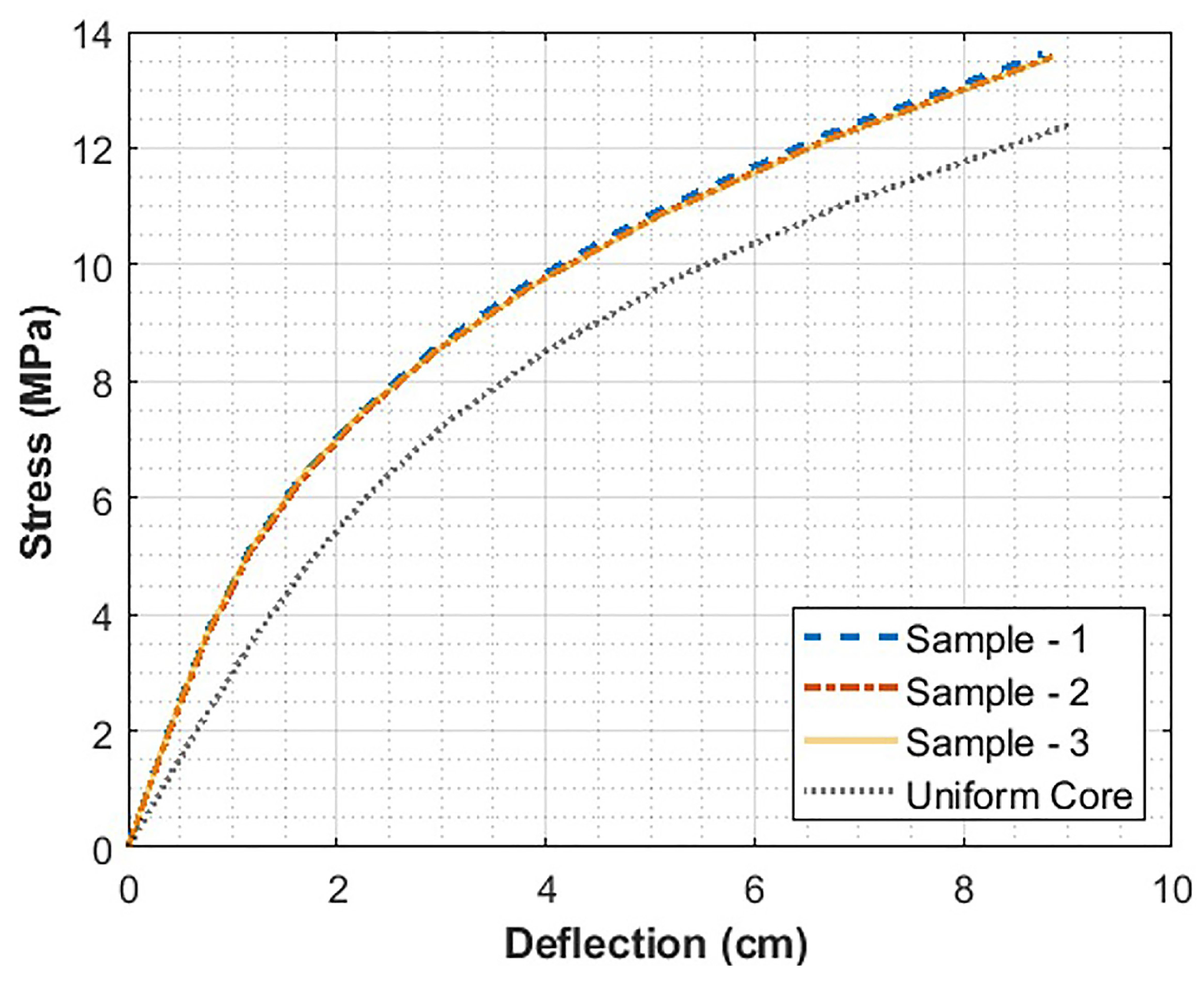
3.2. Finite Element Analysis

The pointwise Young’s modulus was calculated from the spatially varying density using Equation (9) using the data shown in Figure 7c. This spatially varying modulus was then read into COMSOL as discussed in Section 2.4 and the results are presented in Figure 8 for each of the three samples. The Young’s modulus was predicted for the shell region as $E_c$ = 1.73 GPa [39], where, $E_c$ is the Young’s modulus of the HDPE, GFPP composite, and is used for the solid outer shell. Figure 7c and Figure 8 are similar in spatial distribution as the localized density relates to the localized stiffness from Equation (9).

At the boundary between the foamed core and uniform density shell, a linear blending technique was implemented to allow for a smooth and continuous transition of the material properties within the finite element model cross-section. This blend is defined as

$$\begin{array}{c}\hfill E_t=E_s(1-\alpha )+E_f\alpha \end{array}$$

(11)

where $E_f$ is the foamed core modulus calculated using Equation (9) and $E_t$ is the modulus approximated near the transition region around the shell and the core. The constant $\alpha$ is a normalized scalar that linearly increases from 0 to 1, with 0 corresponding to a point fully within the shell region and 1 corresponding to a point within the foamed core region. For the results presented, a transition region of 0.1 inch was taken with the region centered about the transition between the core and the shell.

Performing the FEA simulation for the model discussed in Section 2.4 with the applied load of 111 kN (25,000 lbs), results were plotted to study the load-deflection and stress behavior of the structure. The deflection of the core structure for sample 3 is shown in Figure 9, and the von-Mises stress on the core is superimposed on the deformed structure.

To compare the load-deflection of the four models, the results from samples 1, 2, and 3 were compared to a model that one would obtain if the core had a uniform distribution. The results are shown in Figure 10a and it is observed that all four scenarios yield equivalent results for the overall load-deflection behavior. Equation (12) is used to convert the load to stress and displacement to strain, and the results are shown in Figure 10b.

The plotted stress, S, value is defined in the ASTM standard D6109 and is plotted against the strain r, defined as [44]

$$\begin{array}{c}\hfill S=PL/b{d}^2\\ \hfill r=4.70Dd/L^2\end{array}$$

(12)

where, L is the total span length, b is the width, d is the depth of the beam as shown in Table 2, P is the applied load, and D is the deflection due to the applied load.

The real benefit of the spatially varying cell density homogenization approach allows one to look carefully at the point-wise stress distribution within the core region. Notice in Figure 11a that for the uniform core with no spatial variation, the internal von-Mises stress varies linearly in y with a zero-stress state at the geometric centroid. This behavior changes quickly for the three samples, with spatial variations in the cell density as shown in Figure 11b–d.

Notice that the stress state is no longer a linear function in the vertical dimension, and there are regions where the peak stress is measurably higher within the core than previously. The peak von-Mises stress predicted for sample 3 is a stress value of 13.7 MPa at peak loading, whereas the peak stress in the uniform core is 12.3 MPa for the same loading configuration. There is an ~11% variation in maximum stresses of the samples when compared to the uniform core. Variations in the peak von-Mises stress within the core region at the center-plane of the beam loaded in 4-point bending are shown in Figure 12 as a function of increasing deflection.

It is evident that with each of the different cores, the peak von-Mises stress changes as a function of both cross-head displacement and local cell distribution. It is interesting to note in Figure 12 that there is little difference in the results from the three samples with spatially varying density, but there is a difference in the results with and without spatially varying density. Figure 11a shows the von-Mises stresses with a uniform core, while Figure 11b–d show maximum stress with cores from samples 1–3.

Although the stresses with samples 1–3 have higher stresses overall, the main load and stress are distributed within the outer shell. In addition, the distribution has a relatively smooth transition from the shell to the core, even if there is variability within the core, it is carrying a nominal amount of the overall load. The present study focused mainly on the onset of failure. Various researchers have studied advanced methods for tracking crack propagation within the failed composite (see e.g., [45]), and it is worth studying in future works.

4. Conclusions

In this paper, a method to locally estimate the cell density without the full meshing of the individual cells was presented. This local homogenization was performed using images captured using a digital camera, and a procedure was proposed to analyze the correlation of the cell size and cell distributions to the local stiffness. These results were then fed into a finite element model of a structure subjected to four-point bending. Images taken using a digital camera were analyzed using a custom script written in the MATLAB environment, and an exponential function was proposed to establish a weighting method to allow for a smooth continuous function to be used to represent the local cell variations. This weighted method calculates a density of cells based on their distance from the point analyzed. A periodic boundary was used to estimate the density near the boundaries. Once the local densities were calculated, a micromechanics model that included the constitutive properties of the fiber and matrix along with fiber length and volume fraction of fibers was used to calculate the pointwise Young’s modulus of the core as a function of cell density.

The spatially varying Young’s modulus was then used in a finite element model to analyze the load-deflection of a four-point bend test. These results were compared to a uniform core model previously validated for the macroscopic response to a physical specimen. The macroscopic response for the spatially varying core density and the uniform core density was graphically equivalent. The local von-Mises stress was then analyzed between the two density distribution assumptions, and it was seen that the stresses from the spatially varying cell density resulted in a ∼11% higher stress within the core as compared to the uniform core.

The present study identifies that the spatial variation of the cell distribution within the core impacts the as manufactured performance, but it is unclear from the present work the sensitivity of the final performance on subtle differences in the spatial variations. Future work will consider sectioning multiple regions within the composite structure to study the variability in location, cell size, and distribution, and its impact on final part performance. This method also allows quality control procedures to remain in place without needing an extensive need for equipment and personnel. The ease of taking images and analysis of the proposed method can be extended to other handheld devices like a cell phone or a tablet.

References

1. Bajracharya, R.; Manalo, A.; Karunasena, W.; Lau, K.T. Characterisation of recycled mixed plastic solid wastes: Coupon and full-scale investigation. Waste Manag. 2015, 48, 72–80. [Google Scholar] [CrossRef]
2. Hugo, A.M.; Scelsi, L.; Hodzic, A.; Jones, F.; Dwyer-Joyce, R. Development of recycled polymer composites for structural applications. Plast. Rubber Compos. 2011, 40, 317–323. [Google Scholar] [CrossRef]
3. Grigore, M.E. Methods of Recycling, Properties and Applications of Recycled Thermoplastic Polymers. Recycling 2017, 2, 24. [Google Scholar] [CrossRef] [Green Version]
4. Momanyi, J.; Herzog, M.; Muchiri, P. Analysis of Thermomechanical Properties of Selected Class of Recycled Thermoplastic Materials Based on Their Applications. Recycling 2019, 4, 33. [Google Scholar] [CrossRef] [Green Version]
5. Manalo, A.; Aravinthan, T.; Karunasena, W.; Ticoalu, A. A review of alternative materials for replacing existing timber sleepers. Compos. Struct. 2010, 92, 603–611. [Google Scholar] [CrossRef]
6. Lotfy, I.; Farhat, M.; Issa, M.A.; Al-Obaidi, M. Flexural behavior of high-density polyethylene railroad crossties. Proc. Inst. Mech. Eng. Part F J. Rail Rapid Transit 2016, 230, 813–824. [Google Scholar] [CrossRef]
7. Zyka, K.; Mohajerani, A. Composite piles: A review. Constr. Build. Mater. 2016, 107, 394–410. [Google Scholar] [CrossRef]
8. Jones, R.M. Mechanics of Composite Materials; CRC Press: Boca Raton, FL, USA, 2018. [Google Scholar]
9. Barbeo, E.J. Introduction to Composite Materials Design; CRC Press: Boca Raton, FL, USA, 2017. [Google Scholar]
10. Altan, M. Thermoplastic Foams: Processing, Manufacturing, and Characterization. In Polymerization; IntechOpen: Rijeka, Croatia, 2018; Chapter 6. [Google Scholar]
11. Kord, B.; Varshoei, A.; Chamany, V. Influence of chemical foaming agent on the physical, mechanical, and morphological properties of HDPE/wood flour/nanoclay composites. J. Reinf. Plast. Compos. 2011, 30, 1115–1124. [Google Scholar] [CrossRef]
12. Ruiz, J.A.R.; Vincent, M.; Agassant, J.F.; Sadik, T.; Pillon, C.; Carrot, C. Polymer foaming with chemical blowing agents: Experiment and modeling. Polym. Eng. Sci. 2015, 55, 2018–2029. [Google Scholar] [CrossRef]
13. Carlos, T.C.; Rubén, G.N.; Denis, R. Effect of Mold Temperature on Morphology and Mechanical Properties of Injection Molded HDPE Structural Foams. J. Cell. Plast. 2008, 44, 223–237. [Google Scholar]
14. Yousefian, H.; Rodrigue, D. Nano-crystalline cellulose, chemical blowing agent, and mold temperature effect on morphological, physical/mechanical properties of polypropylene. J. Appl. Polym. Sci. 2015, 132. [Google Scholar] [CrossRef]
15. Tissandier, C.; González-Núñez, R.; Rodrigue, D. Asymmetric microcellular composites: Morphological properties. J. Cell. Plast. 2014, 50, 449–473. [Google Scholar] [CrossRef]
16. Villamizar, C.A.; Han, C.D. Studies on structural foam processing II. Bubble dynamics in foam injection molding. Polym. Eng. Sci. 1978, 18, 699–710. [Google Scholar] [CrossRef]
17. González-Núñez, R. Microcellular Agave Fibre-High Density Polyethylene Composites Produced By Injection Molding. J. Mater. Sci. Eng. 2012, 2, 667–692. [Google Scholar]
18. Redenbach, C.; Shklyar, I.; Andrae, H. Laguerre tessellations for elastic stiffness simulations of closed foams with strongly varying cell sizes. Int. J. Eng. Sci. 2012, 50, 70–78. [Google Scholar] [CrossRef]
19. Barbier, C.; Michaud, P.; Baillis, D.; Randrianalisoa, J.; Combescure, A. New laws for the tension/compression properties of Voronoi closed-cell polymer foams in relation to their microstructure. Eur. J. Mech. A/Solids 2014, 45, 110–122. [Google Scholar] [CrossRef]
20. Zhang, Y.; Rodrigue, D.; Ait-Kadi, A. High Density Polyethylene Foams. II. Elastic Modulus. J. Appl. Polym. Sci. 2003, 90, 2120–2129. [Google Scholar] [CrossRef]
21. Mori, T.; Tanaka, K. Average Stress in Matrix and Average Elastic Energy of Materials With Misfitting Inclusions. Acta Metall. 1973, 21, 571–574. [Google Scholar] [CrossRef]
22. Weng, G. Some elastic properties of reinforced solids, with special reference to isotropic ones containing spherical inclusions. Int. J. Eng. Sci. 1984, 22, 845–856. [Google Scholar] [CrossRef]
23. Farber, J.; Farris, J. Model for prediction of the elastic response of reinforced materials over wide ranges of concentration. J. Appl. Polym. Sci. 1987, 34, 2093–2104. [Google Scholar] [CrossRef]
24. McLaughlin, R. A study of the differential scheme for composite materials. Int. J. Eng. Sci. 1977, 15, 237–244. [Google Scholar] [CrossRef]
25. Gibson, L.J.; Ashby, M.F. Cellular Solids: Structure and Properties; Cambridge University Press: Cambridge, UK, 1997. [Google Scholar]
26. Moore, D.; Iremonger, M. The Prediction of the Flexural Rigidity of Sandwich Foam Mouldings. J. Cell. Plast. 1974, 10, 230–236. [Google Scholar] [CrossRef]
27. Lo, K.H.; Miyase, A.; Wang, S.S. Stiffness predictions for closed-cell PVC foams. J. Compos. Mater. 2016, 51, 3327–3336. [Google Scholar] [CrossRef]
28. Tucker, C.L., III; Liang, E. Stiffness Predictions for Unidirectional Short-Fiber Composites: Review and Evaluation. Compos. Sci. Technol. 1999, 59, 655–671. [Google Scholar] [CrossRef]
29. Tandon, G.; Weng, G.J. The effect of aspect ratio on the elastic properties of unidirectionally aligned composites. Polym. Compos. 1984, 5, 327–333. [Google Scholar] [CrossRef]
30. Zhang, C. Modeling of Flexible Fiber Motion and Prediction of Material Properties. Master’s Thesis, Baylor University, Waco, TX, USA, 2011. [Google Scholar]
31. Barzegari, M.; Rodrigue, D. Tensile Modulus Prediction of Structural Foams using Density Profiles. Cell. Polym. 2008, 27, 285–301. [Google Scholar] [CrossRef]
32. Davari, M.; Razavi Aghjeh, M.K.; Seraji, S. Relationship between the cell structure and mechanical properties of chemically crosslinked polyethylene foams. J. Appl. Polym. Sci. 2012, 124, 2789–2797. [Google Scholar] [CrossRef]
33. Sadik, T.; Pillon, C.; Carrot, C.; Reglero Ruiz, J.; Vincent, M.; Billon, N. Polypropylene structural foams: Measurements of the core, skin, and overall mechanical properties with evaluation of predictive models. J. Cell. Plast. 2016, 53, 25–44. [Google Scholar] [CrossRef]
34. Shen, H.; Oppenheimer, S.; Dunand, D.; Brinson, L. Numerical Modelling of Pore Size Distribution in Foamed Titanium. Mech. Mater. 2006, 38, 933–944. [Google Scholar] [CrossRef] [Green Version]
35. Chen, Y.; Das, R.; Battley, M. Effects of cell size and cell wall thickness variations on the stiffness of closed-cell foams. Int. J. Solids Struct. 2015, 52, 150–164. [Google Scholar] [CrossRef]
36. Zhu, X.; Ai, S.; Fang, D.; Liu, B.; Lu, X. A novel modeling approach of aluminum foam based on MATLAB image processing. Comput. Mater. Sci. 2014, 82, 451–456. [Google Scholar] [CrossRef]
37. Nasrabadi, A.M.; Hedayati, R.; Sadighi, M. Numerical and experimental study of the mechanical response of aluminum foams under compressive loading using CT data. J. Theor. Appl. Mech. 2016, 54, 1357–1368. [Google Scholar] [CrossRef] [Green Version]
38. Yunus, S.; Sefa-Ntiri, B.; Anderson, B.; Kumi, F.; Mensah-Amoah, P.; Sonko Sackey, S. Quantitative Pore Characterization of Polyurethane Foam with Cost-Effective Imaging Tools Image Analysis: A Proof-Of-Principle Study. Polymers 2019, 11, 1879. [Google Scholar] [CrossRef] [PubMed] [Green Version]
39. Pulipati, D.P.; Jack, D.A. Characterization and model validation for large format chopped fiber, foamed, composite structures made from recycled olefin based polymers. Polymers 2020, 12, 1371. [Google Scholar] [CrossRef] [PubMed]
40. Pinto, J.; Solórzano, E.; Rodríguez-Pérez, M.; De Saja, J. Characterization of the cellular structure based on user-interactive image analysis procedures. J. Cell. Plast. 2013, 49, 554–574. [Google Scholar] [CrossRef]
41. Advani, S.G.; Tucker, C.L., III. The use of tensors to describe and predict fiber orientation in short fiber composites. J. Rheol. 1987, 31, 751–784. [Google Scholar] [CrossRef]
42. VerWeyst, B.E.; Tucker, C.L., III. Fiber suspensions in complex geometries: Flow-orientation coupling. Can. J. Chem. Eng. 2002, 80, 1093–1106. [Google Scholar] [CrossRef]
43. Ramberg, W.; Osgood, W.R. Description of Stress-Strain Curves by three Parameters; Technical Note No. 902; National Aeronautics and Space Administration: Washington, DC, USA, 1943.
44. Flexural Properties of Unreinforced and Reinforced Plastic Lumber and Related Products. In Standard Test Methods; ASTM International: West Conshohocken, PA, USA, 2013.
45. Mehrmashhadi, J.; Chen, Z.; Zhao, J.; Bobaru, F. A stochastically homogenized peridynamic model for intraply fracture in fiber-reinforced composites. Compos. Sci. Technol. 2019, 182, 107770. [Google Scholar] [CrossRef]
Figure 1. Example of a cross-section.
Jcs 04 00093 g001
Figure 2. Cross-section of the presented samples. (a) Images of sample 1, 2, and 3 from the commercial off-the-shelf (COTS) camera. (b) Binary plots of samples 1, 2, and 3.
Jcs 04 00093 g002
Figure 3. Image processing false positives. (a) Image with a yellow tint showing color contrasts within cells. (b) Pixel formation of cell donuts based on color contrast. (c) Cells with double circles. (d) Filtering the image of double circles.
Jcs 04 00093 g003
Figure 4. Cell area validation using a Keyence digital microscope. (a) Measuring diameter as seen from the Keyence microscope. (b) Measuring the effective diameter of the same cell using the new proposed method. (c) Manually measuring the area of each cell using the Keyence microscope. (d) Automated measuring of the effective diameters of all the cells.
Jcs 04 00093 g004
Figure 5. Mirrored image preventing image biasing near the boundaries. A single grid point is highlighted, showing the region of consideration used for local density homogenization.
Jcs 04 00093 g005
Figure 6. Quadrilateral Mesh for various surfaces of the symmetric FEA model.
Jcs 04 00093 g006
Figure 7. Various stages within the MATLAB image processing technique. (a) Cell area identification for samples 1 through 3. (b) Histograms of the cell size distribution for samples 1 through 3. (c) Spatially varying effective local density for samples 1 through 3 within the foamed core.
Jcs 04 00093 g007
Figure 8. Spatially varying Young’s modulus obtained from image analysis for (a) sample 1, (b) sample 2, (c) sample 3.
Jcs 04 00093 g008
Figure 9. FEA results for core stress under deformation for sample 3.
Jcs 04 00093 g009
Figure 10. Results from FEA (a) comparing load–deflection from various samples and (b) comparing stress–deflection from various samples.
Jcs 04 00093 g010
Figure 11. Core von-Mises stress at mid-point for each four-point bend simulation in the units of MPa for (a) uniform core, (b) sample 1, (c) sample 2, and (d) sample 3.
Jcs 04 00093 g011
Figure 12. Stress comparison for the various FEA models with image cross-sections and the uniform core.
Jcs 04 00093 g012