Peridynamic Mindlin Plate Formulation for Functionally Graded Materials

Abstract

In this study, a new peridynamic Mindlin plate formulation is presented which is suitable for the analysis of functionally graded materials. The governing equations of peridynamic formulation are obtained by using Euler-Lagrange equations in conjunction with Taylor’s expansion. To validate the new formulation, three different numerical benchmark problems are considered for a Mindlin plate subjected to simply supported, fully clamped and mixed (clamped-simply supported) boundary conditions. Peridynamic results are compared against results from finite element analysis and a good agreement is observed between the two methods.

1. Introduction

As the manufacturing technology advances, it becomes possible to design materials that have better properties with respect to traditional materials including metals and fibre-reinforced composite materials. Usage of fibre-reinforced composite materials is increasing in different industries including automotive, aerospace and marine fields. Although fibre-reinforced composite materials are light, have good impact properties and corrosion resistance, they suffer from delamination damage occurring between neighbouring plies which significantly reduces the load carrying capacities of these materials. Delamination damage can be avoided by continuously varying material properties in the form of functionally graded materials.

There are currently numerous studies in the literature focusing on plate formulations of functionally graded materials. Amongst these Vel and Batra [1] provided three-dimensional exact solution for the vibration of functionally graded rectangular plates. Shen [2] obtained nonlinear bending response of functionally graded plates subjected to transverse loading by using Reddy’s higher order shear deformation plate theory. Zenkour [3] presented generalised shear deformation theory for bending analysis of functionally graded plates. Bian et. al. [4] derived analytical solutions for functionally graded plates under cylindrical bending using first- and third-order shear deformation theories. Carrera et. al. [5] investigated the effect of thickness stretching in functionally graded plates by using Carrera’s Unified Formulation. Ferreira et. al. [6] used meshless method and third-order shear deformation theory to analyse functionally graded plates. Kashtalyan [7] utilised Plevako general solution of the equilibrium equations for inhomogeneous isotropic media to obtain three-dimensional elasticity solution for functionally graded simply supported plates. Xiang and Kang [8] performed bending analysis of functionally graded plates by using nth-order shear deformation theory and meshless global collocation method based on the thin plate spline radial basis function.

In this study, an alternative formulation is presented using peridynamics [9,10,11,12,13,14,15,16,17,18,19,20,21,22,23,24,25,26,27,28,29] to analyse functionally graded plates based on Mindlin plate theory by taking into account transverse shear deformation. Peridynamics (PD) is a new continuum mechanics formulation. PD equations are in the form of integro-differential equations which do not contain spatial derivatives which makes it convenient for analysing cracks. Moreover, it has a length scale parameter that can allow analysing problems that cannot be represented by using classical formulations. On the other hand, partial differential equations are used in Refs. [1,2,3,4,5,6,7,8] and they do not contain length scale parameters. Since its introduction, there has been a rapid progress on peridynamics especially in the recent years. PD has been used to analyse different material systems such as metals [30], composites [31], functionally graded materials [32], concrete [33], graphene [34], etc. PD is not limited to elasticity, but can represent plastic [35], viscoelastic [36] and viscoplastic [37] material behaviour. Moreover, in addition to structural analysis, PD can also be used for the analysis of other fields including heat transfer [38], moisture diffusion [39], porous flow [40], etc. Simplified structures such as beams, plates and shells can also be represented in PD framework. Taylor and Steigmann [41] developed PD formulation for thin plates. Non-ordinary state-based Euler beam [42] and Kirchhoff plate [43] formulations were presented by O’Grady and Foster. To analyse relatively thick plates, Diyaroglu et. al. [44] introduced PD Timoshenko and Mindlin plate formulations by taking into account transverse shear deformations. This study only considers isotropic materials and Mindlin plate formulation is limited to a constant Poisson’s ratio of 1/3. Chowdhury et al. [45] introduced PD formulation for linear elastic shells. Note that there are fundamental differences between peridynamics and other non-local continuum mechanics approaches such as Eringen’s non-local elasticity formulation. Please refer to Madenci and Oterkus [46] for more information about the fundamentals of peridynamic theory. An extensive review of peridynamic research is given in Javili et al. [47]. To obtain governing equations of peridynamic Mindlin plate formulation for functionally graded materials Euler-Lagrange equations in conjunction with Taylor’s expansion are utilised. The formulation does not have any limitation on material constants as in bond-based peridynamics. To validate the current formulation, several benchmark problems are considered and peridynamic results are compared against results from finite element analysis.

2. Classical Mindlin Plate Formulation

Mindlin plate formulation was developed to analyse relatively thick plates by taking into account transverse shear deformations which is neglected in Kirchhoff plate theory suitable for thin plates. According to Mindlin plate theory, the displacement of a material point can be expressed in terms of displacement and rotation fields of the material points along the mid-plane (xy-plane)

$$u\left(x,y,z,t\right)=u\left(x,y,0,t\right)+z{\theta }_x\left(x,y,0,t\right)$$

(1a)

$$v\left(x,y,z,t\right)=v\left(x,y,0,t\right)+z{\theta }_y\left(x,y,0,t\right)$$

(1b)

$$w\left(x,y,z,t\right)=w\left(x,y,0,t\right)$$

(1c)

where ${\theta }_x\left(x,y,0,t\right)$ and ${\theta }_y\left(x,y,0,t\right)$ denote the rotation of the material points on the mid-plane about positive y-direction and negative x-direction, respectively. Hereafter, $u\left(x,y,0,t\right)$, $v\left(x,y,0,t\right)$, $w\left(x,y,0,t\right)$, ${\theta }_x\left(x,y,0,t\right)$ and ${\theta }_y\left(x,y,0,t\right)$ are written simply as $u$, $v$, $w$, ${\theta }_x$ and ${\theta }_y$, respectively. The positive set of the degrees-of-freedom is shown in Figure 1.

Thus, the strain-displacement relationship can be written as

$${\epsilon }_{xx}=\frac{\partial u}{\partial x}+z\frac{\partial {\theta }_x}{\partial x}$$

(2a)

$${\epsilon }_{yy}=\frac{\partial v}{\partial y}+z\frac{\partial {\theta }_y}{\partial y}$$

(2b)

$${\epsilon }_{xy}={\epsilon }_{yx}=\frac{1}{2}\left[\left(\frac{\partial u}{\partial y}+\frac{\partial u}{\partial x}\right)+z\left(\frac{\partial {\theta }_x}{\partial y}+\frac{\partial {\theta }_y}{\partial x}\right)\right]$$

(2c)

$${\gamma }_{xz}={\kappa }_s\left({\theta }_x+\frac{\partial w}{\partial x}\right)$$

(2d)

$${\gamma }_{yz}={\kappa }_s\left({\theta }_y+\frac{\partial w}{\partial y}\right)$$

(2e)

$${\epsilon }_{zz}=0$$

(2f)

which can be also expressed in terms of indicial notation as

$${\epsilon }_{IJ}=\frac{1}{2}\left[\left(\frac{\partial u_I}{\partial x_J}+\frac{\partial u_J}{\partial x_I}\right)+z\left(\frac{\partial {\theta }_I}{\partial x_J}+\frac{\partial {\theta }_J}{\partial x_I}\right)\right]$$

(3a)

$${\gamma }_{I3}={\kappa }_s\left({\theta }_I+\frac{\partial w}{\partial x_I}\right)$$

(3b)

where ${\kappa }_s$ is introduced as shear coefficient. Note that the subscript indices, $I,J,\cdots =1\left(=x\right),2\left(=y\right)$, and this convention will be applied throughout this study.

For planar isotropic materials, the stress–strain relationships can be written as:

$${\sigma }_{xx}=\frac{E\left(z\right)}{1-\nu {\left(z\right)}^2}\left({\epsilon }_{xx}+\nu {\epsilon }_{yy}\right)$$

(4a)

$${\sigma }_{yy}=\frac{E\left(z\right)}{1-\nu {\left(z\right)}^2}\left({\epsilon }_{yy}+\nu {\epsilon }_{xx}\right)$$

(4b)

$${\sigma }_{xy}=\frac{E\left(z\right)}{2\left(1+\nu \left(z\right)\right)}\left({\epsilon }_{xy}+{\epsilon }_{yx}\right)$$

(4c)

$${\tau }_{xz}=G\left(z\right){\gamma }_{xz}$$

(4d)

$${\tau }_{yz}=G\left(z\right){\gamma }_{yz}$$

(4e)

where $G=\frac{E\left(z\right)}{2\left(1+\nu \left(z\right)\right)}$ is the shear modulus.

Note that the transverse normal stress, ${\sigma }_{zz}$, is considered to be small compared to in-plane stresses. Thus, it is discarded from the stress components set and this simplifies the 3-dimensional Hooke’s law and makes it a 2-dimensional plane-stress material constitutive law. The stress components can also be expressed in indicial notation as:

$${\sigma }_{IJ}=C_{IJKL}{\epsilon }_{KL}$$

(5a)

$${\tau }_{I3}=G\left(z\right){\gamma }_{I3}$$

(5b)

where in-plane stiffness tensor can be defined as

$$C_{IJKL}=\frac{E\left(z\right)}{1-\nu {\left(z\right)}^2}\left[\frac{1-\nu \left(z\right)}{2}\left({\delta }_{IL}{\delta }_{JK}+{\delta }_{IK}{\delta }_{JL}\right)+\nu \left(z\right){\delta }_{IJ}{\delta }_{KL}\right]$$

(6)

The strain energy per unit area of the plate can be casted as:

$$W={{\displaystyle \int }}_{-\frac{h}{2}}^{\frac{h}{2}}\frac{1}{2}\left({\sigma }_{IJ}{\epsilon }_{IJ}+{\tau }_{I3}{\gamma }_{I3}\right)dz$$

(7)

where $h$ represents the thickness of the plate. Inserting Equations (3), (5) and (6) into (7) and rearranging indices yields

$$W=\frac{1}{2}{{\displaystyle \int }}_{-\frac{h}{2}}^{\frac{h}{2}}\left(\frac{E\left(z\right)}{1-\nu {\left(z\right)}^2}\left[\left(1-\nu \left(z\right)\right){\epsilon }_{IJ}{\epsilon }_{IJ}+\nu \left(z\right){\epsilon }_{JJ}{\epsilon }_{II}\right]+G\left(z\right){\gamma }_{I3}{\gamma }_{I3}\right)dz$$

(8a)

or

$$\begin{array}{ll}W={{\displaystyle \int }}_{-\frac{h}{2}}^{\frac{h}{2}}\frac{G\left(z\right)}{2}dz& \left(\frac{\partial u_I}{\partial x_J}\frac{\partial u_I}{\partial x_J}+\frac{\partial u_I}{\partial x_J}\frac{\partial u_J}{\partial x_I}+\frac{\partial u_I}{\partial x_I}\frac{\partial u_J}{\partial x_J}\right)\\ & +{{\displaystyle \int }}_{-\frac{h}{2}}^{\frac{h}{2}}\frac{G\left(z\right)}{2}{z}^{2}dz\left(\frac{\partial {\theta }_I}{\partial x_J}\frac{\partial {\theta }_I}{\partial x_J}+\frac{\partial {\theta }_I}{\partial x_J}\frac{\partial {\theta }_J}{\partial x_I}+\frac{\partial {\theta }_I}{\partial x_I}\frac{\partial {\theta }_J}{\partial x_J}\right)\\ & +{{\displaystyle \int }}_{-\frac{h}{2}}^{\frac{h}{2}}G\left(z\right)zdz\left(\frac{\partial u_I}{\partial x_J}\frac{\partial {\theta }_I}{\partial x_J}+\frac{\partial {\theta }_I}{\partial x_J}\frac{\partial u_J}{\partial x_I}+\frac{\partial u_I}{\partial x_I}\frac{\partial {\theta }_J}{\partial x_J}\right)\\ & +({{\displaystyle \int }}_{-\frac{h}{2}}^{\frac{h}{2}}G\left(z\right)\frac{3\nu \left(z\right)-1}{2\left[1-\nu \left(z\right)\right]}dz\frac{\partial u_I}{\partial x_I}\frac{\partial u_J}{\partial x_J}\\ & +{{\displaystyle \int }}_{-\frac{h}{2}}^{\frac{h}{2}}G\left(z\right)\frac{3\nu \left(z\right)-1}{2\left[1-\nu \left(z\right)\right]}{z}^{2}dz\frac{\partial {\theta }_I}{\partial x_I}\frac{\partial {\theta }_J}{\partial x_J}\\ & +{{\displaystyle \int }}_{-\frac{h}{2}}^{\frac{h}{2}}G\left(z\right)\frac{3\nu \left(z\right)-1}{1-\nu \left(z\right)}zdz\frac{\partial u_I}{\partial x_I}\frac{\partial {\theta }_J}{\partial x_J})\\ & +{{\displaystyle \int }}_{-\frac{h}{2}}^{\frac{h}{2}}{\kappa }_s^2\frac{G\left(z\right)}{2}dz\left({\theta }_I+\frac{\partial w}{\partial x_I}\right)\left({\theta }_I+\frac{\partial w}{\partial x_I}\right)\end{array}$$

(8b)

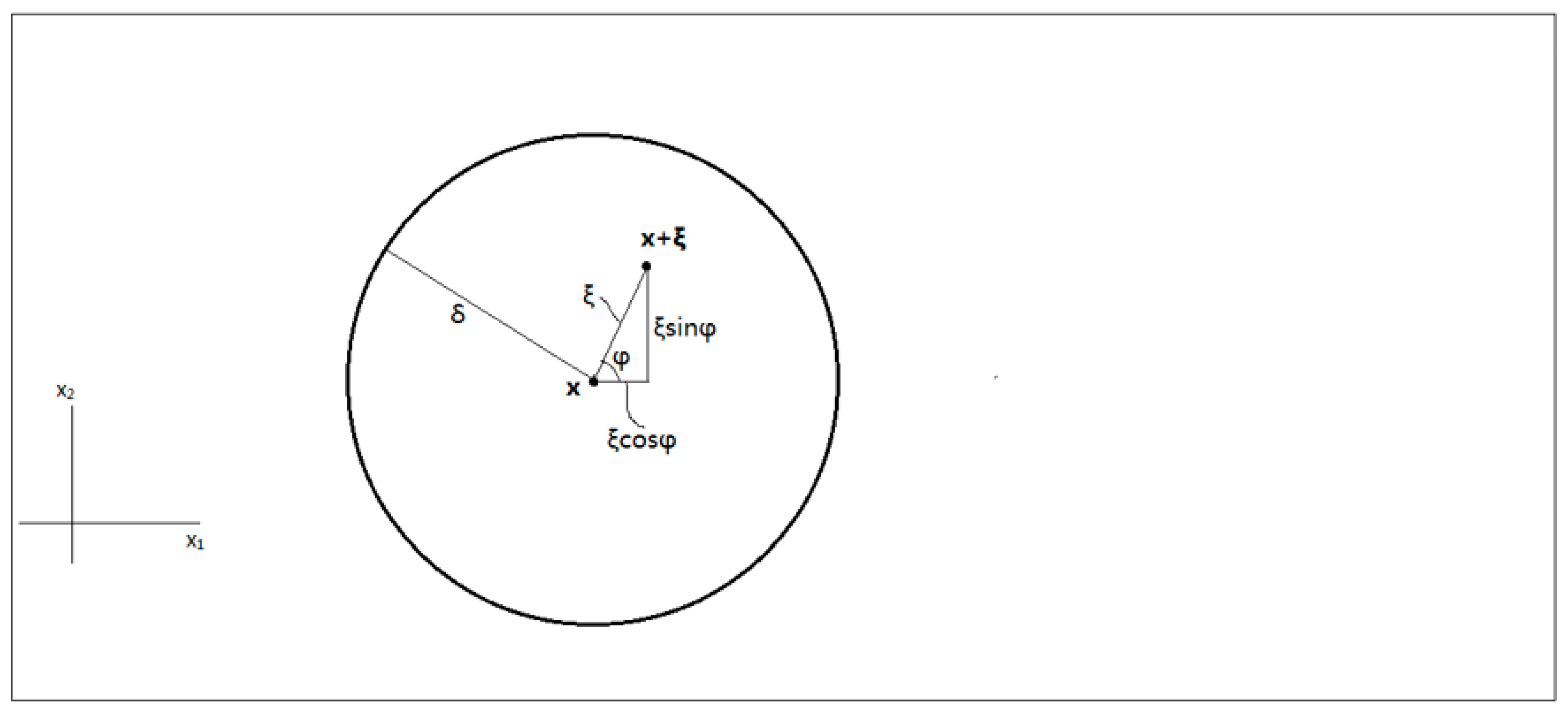
3. Peridynamic Mindlin Plate Formulation

Peridynamics (PD) is a non-local continuum mechanics formulation. Therefore, material points inside the solution domain can interact with each other material points in a non-local manner. The range of non-local interactions is defined as ‘horizon’, $H$. The equations of motion of peridynamics can be written as

$$\rho \left(\mathit{x}\right)\ddot{\mathit{u}}\left(\mathit{x},t\right)={{\displaystyle \int }}_H^{}\left(\mathit{t}-{\mathit{t}}^{\prime }\right)d{V}^{\prime }+\mathit{b}\left(x,t\right)$$

(9)

or in discrete form for the material point $k$ as

$${\rho }_{\left(k\right)}{\ddot{\mathit{u}}}_{\left(k\right)}={\displaystyle \sum }_{j=1}^N\left({\mathit{t}}_{\left(k\right)\left(j\right)}-{\mathit{t}}_{\left(j\right)\left(k\right)}\right)V_{\left(j\right)}+{\mathit{b}}_{\left(k\right)}$$

(10)

where ${\mathit{t}}_{\left(k\right)\left(j\right)}$ and ${\mathit{t}}_{\left(j\right)\left(k\right)}$ are the peridynamic force densities between two material points k and j as shown in Figure 2 and N is the number of material points inside the horizon. Note that the PD equations of motion given in Equations (9) and (10) have the same form as in classical continuum mechanics except the integration or summation term.

The PD equations of motion can be derived by utilising Euler-Lagrange’s equation:

$$\frac{d}{dt}\frac{\partial L}{\partial {\dot{\mathit{u}}}_{\left(k\right)}}-\frac{\partial L}{\partial {\mathit{u}}_{\left(k\right)}}=0$$

(11)

where $L=T-U$ is the Lagrangian. The kinetic energy per unit area, $\overline{T}$, can be expressed as

$$\overline{T}=\frac{1}{2}{{\displaystyle \int }}_{-\frac{h}{2}}^{\frac{h}{2}}\rho \dot{\mathit{u}}\left(x,y,z,t\right)·\dot{\mathit{u}}\left(x,y,z,t\right)dz$$

(12)

where $u$ is the generalised displacement vector, which in this study can be defined as

$$u={\left(\begin{array}{cc}{u}_1& \begin{array}{cc}{u}_2& \begin{array}{cc}{\theta }_1& \begin{array}{cc}{\theta }_2& w\end{array}\end{array}\end{array}\end{array}\right)}^T$$

(13)

Substituting Equation (1) into Equation (12) results in

$$\begin{gathered} \overline{T}=\frac{1}{2}{{\displaystyle \int }}_{-\frac{h}{2}}^{\frac{h}{2}}\rho \left[\left({\dot{u}}_1^2+{\dot{u}}_2^2\right)+z^2\left({\dot{\theta }}_1^2+{\dot{\theta }}_2^2\right)+2z\left({\dot{u}}_1{\dot{\theta }}_1+{\dot{u}}_2{\dot{\theta }}_2\right)+{\dot{w}}^2\right]dz \\ =\frac{1}{2}\rho \left[h\left({\dot{u}}_1^2+{\dot{u}}_2^2+{\dot{w}}^2\right)+\frac{h^3}{12}\left({\dot{\theta }}_1^2+{\dot{\theta }}_2^2\right)\right] \end{gathered}$$

(14)

The total kinetic energy of the body can be casted by integrating Equation (14) over the whole mid-plane as

$$T={{\displaystyle \int }}_A^{}\overline{T}dA=\frac{1}{2}{{\displaystyle \int }}_A\rho \left[\frac{h^3}{12}\left({\dot{\theta }}_1^2+{\dot{\theta }}_2^2\right)+h\left({\dot{u}}_1^2+{\dot{u}}_2^2+{\dot{w}}^2\right)\right]dA$$

(15a)

which can be written in discretised form as

$$\begin{array}{cc}T={\displaystyle {\displaystyle \sum }_k}{\overline{T}}_{\left(k\right)}{A}_{\left(k\right)}& =\frac{1}{2}{\displaystyle {\displaystyle \sum }_k}{\rho }_{\left(k\right)}[\frac{h^3}{12}{\left({\dot{\theta }}_1^{\left(k\right)}\right)}^2+\frac{h^3}{12}{\left({\dot{\theta }}_2^{\left(k\right)}\right)}^2\\ & +h\left({\left({\dot{u}}_1^{\left(k\right)}\right)}^2+{\left({\dot{u}}_2^{\left(k\right)}\right)}^2+{\dot{w}}_{\left(k\right)}^2\right)]A_{\left(k\right)}\end{array}$$

(15b)

where $A_{\left(k\right)}$ is the area that contains the material point $k$.

The PD strain energy density function has a non-local form such that the strain energy of a certain material point $k$ depends on both its displacement and all other material points in its family, which can be expressed as

$$W_{\left(k\right)}=W_{\left(k\right)}\left({\mathit{u}}_{\left(k\right)}, {\mathit{u}}_{\left(1^k\right)}, {\mathit{u}}_{\left(2^k\right)}, {\mathit{u}}_{\left(3^k\right)}, \cdots \right)$$

(16)

where ${\mathit{u}}_{\left(k\right)}$ is the displacement vector of material point $k$ and ${\mathit{u}}_{\left(i^k\right)}$ ($i=1, 2, 3, \cdots$) is the displacement vector of the $i$th material point within the horizon of the material point $k$.

Similar to Equation (15), the total potential energy stored in the body can be obtained by summing potential energies of all material points including strain energy and energy due to external loads as

$$U={\displaystyle \sum }_k{W}_{\left(k\right)}\left({\mathit{u}}_{\left(k\right)}, {\mathit{u}}_{\left(1^k\right)}, {\mathit{u}}_{\left(2^k\right)}, {\mathit{u}}_{\left(3^k\right)}, \cdots \right)A_{\left(k\right)}-{\displaystyle \sum }_k{\mathit{b}}_{\left(k\right)}{\mathit{u}}_{\left(k\right)}{A}_{\left(k\right)}$$

(17)

where $\mathbf{b}$ is the body force density vector, which in this study has the following components

$$b={\left(\begin{array}{cc}{b}_{u_1}& \begin{array}{cc}{b}_{u_2}& \begin{array}{cc}{b}_{{\theta }_1}& \begin{array}{cc}{b}_{{\theta }_2}& b_z\end{array}\end{array}\end{array}\end{array}\right)}^T$$

(18)

with $b_u$, $b_{\theta }$ and $b_z$ correspond to in-plane loads, moments and transverse body loads, respectively.

The first term of the Euler-Lagrange’s equation can be obtained by inserting Equations (15b) and (17) into Equation (11) as

$$\frac{d}{dt}\frac{\partial L}{\partial {\dot{\mathit{u}}}_{\left(k\right)}}=\frac{d}{dt}\frac{\partial T}{\partial {\dot{\mathit{u}}}_{\left(k\right)}}={\rho }_{\left(k\right)}\left\{\begin{array}{c}\begin{array}{c}\begin{array}{c}h{\ddot{u}}_1^{\left(k\right)}\\ h{\ddot{u}}_2^{\left(k\right)}\end{array}\\ \frac{h^3}{12}{\ddot{\theta }}_1^{\left(k\right)}\end{array}\\ \frac{h^3}{12}{\ddot{\theta }}_2^{\left(k\right)}\\ h{\ddot{w}}_{\left(k\right)}\end{array}\right\}{A}_{\left(k\right)}$$

(19)

Similarly, the second term of the Euler-Lagrange’s equation becomes

$$\begin{array}{ll}-\frac{\partial L}{\partial {\mathit{u}}_{\left(k\right)}}=\frac{\partial U}{\partial {\mathit{u}}_{\left(k\right)}}& =\frac{\partial }{\partial {\mathit{u}}_{\left(k\right)}}{\displaystyle {\displaystyle \sum }_n}{W}_{\left(n\right)}\left({\mathit{u}}_{\left(n\right)}, {\mathit{u}}_{\left(1^n\right)}, {\mathit{u}}_{\left(2^n\right)}, {\mathit{u}}_{\left(3^n\right)}, \cdots \right)A_{\left(n\right)}\\ & -\frac{\partial }{\partial {\mathit{u}}_{\left(k\right)}}{\displaystyle {\displaystyle \sum }_n}{\mathit{b}}_{\left(n\right)}{\mathit{u}}_{\left(n\right)}{A}_{\left(n\right)}\\ & ={\displaystyle {\displaystyle \sum }_n}\frac{\partial W_{\left(n\right)}}{\partial {\mathit{u}}_{\left(k\right)}}\left({\delta }_{nk}+{\delta }_{n{i}^k}\right)A_{\left(n\right)}-{\displaystyle {\displaystyle \sum }_n}{\mathit{b}}_{\left(n\right)}{\delta }_{nk}{A}_{\left(n\right)}\\ & =\left(\frac{\partial W_{\left(k\right)}}{\partial {\mathit{u}}_{\left(k\right)}}{A}_{\left(k\right)}+{\displaystyle {\displaystyle \sum }_j}\frac{\partial W_{\left(j\right)}}{\partial {\mathit{u}}_{\left(k\right)}}{A}_{\left(j\right)}\right)-{\mathit{b}}_{\left(k\right)}{A}_{\left(k\right)}\end{array}$$

(20)

Inserting Equations (19) and (20) into the Euler-Lagrange’s equation yields:

$${\rho }_{\left(k\right)}\left\{\begin{array}{c}\begin{array}{c}\begin{array}{c}h{\ddot{u}}_1^{\left(k\right)}\\ h{\ddot{u}}_2^{\left(k\right)}\end{array}\\ \frac{h^3}{12}{\ddot{\theta }}_1^{\left(k\right)}\end{array}\\ \frac{h^3}{12}{\ddot{\theta }}_2^{\left(k\right)}\\ h{\ddot{w}}_{\left(k\right)}\end{array}\right\}{A}_{\left(k\right)}=-\left\{\begin{array}{c}\frac{\partial W_{\left(k\right)}}{\partial u_1^{\left(k\right)}}{A}_{\left(k\right)}+{\displaystyle {\displaystyle \sum }_j}\frac{\partial W_{\left(j\right)}}{\partial u_1^{\left(k\right)}}{A}_{\left(j\right)}\\ \frac{\partial W_{\left(k\right)}}{\partial u_2^{\left(k\right)}}{A}_{\left(k\right)}+{\displaystyle {\displaystyle \sum }_j}\frac{\partial W_{\left(j\right)}}{\partial u_2^{\left(k\right)}}{A}_{\left(j\right)}\\ \frac{\partial W_{\left(k\right)}}{\partial {\theta }_1^{\left(k\right)}}{A}_{\left(k\right)}+{\displaystyle {\displaystyle \sum }_j}\frac{\partial W_{\left(j\right)}}{\partial {\theta }_1^{\left(k\right)}}{A}_{\left(j\right)}\\ \frac{\partial W_{\left(k\right)}}{\partial {\theta }_2^{\left(k\right)}}{A}_{\left(k\right)}+{\displaystyle {\displaystyle \sum }_j}\frac{\partial W_{\left(j\right)}}{\partial {\theta }_2^{\left(k\right)}}{A}_{\left(j\right)}\\ \frac{\partial W_{\left(k\right)}}{\partial W_{\left(k\right)}}{A}_{\left(k\right)}+{\displaystyle {\displaystyle \sum }_j}\frac{\partial W_{\left(j\right)}}{\partial W_{\left(k\right)}}{A}_{\left(j\right)}\end{array}\right\}+\left\{\begin{array}{c}\begin{array}{c}\begin{array}{c}{b}_{u_1}^{\left(k\right)}\\ b_{u_2}^{\left(k\right)}\end{array}\\ b_{{\theta }_1}^{\left(k\right)}\end{array}\\ b_{{\theta }_2}^{\left(k\right)}\\ b_z^{\left(k\right)}\end{array}\right\}{A}_{\left(k\right)}$$

(21)

In order to write the non-local form of strain energy function of the material point $k$, Equation (8b), it is necessary to transform all the local terms into an equivalent PD form by also considering PD strain energy expression given in Equation (16). As derived in Appendix A, the strain energy density function of the material point $k$ and its family member $j$ can be expressed as

$$\begin{array}{l}{W}_{\left(k\right)}\\ =\frac{12}{\pi {\delta }^3}({{\displaystyle \int }}_{-\frac{h}{2}}^{\frac{h}{2}}\frac{G\left(z\right)}{2}dz{\displaystyle {\displaystyle \sum }_i^{}}\frac{{\left[\left(u_I^{\left(i^k\right)}-u_I^{\left(k\right)}\right)n_I^{\left(i^k\right)\left(k\right)}\right]}^2}{{\xi }_{\left(i^k\right)\left(k\right)}}{A}_{\left(i^k\right)}\\ +{{\displaystyle \int }}_{-\frac{h}{2}}^{\frac{h}{2}}\frac{G\left(z\right)}{2}{z}^{2}dz{\displaystyle {\displaystyle \sum }_i^{}}\frac{{\left[\left({\theta }_I^{\left(i^k\right)}-{\theta }_I^{\left(k\right)}\right)n_I^{\left(i^k\right)\left(k\right)}\right]}^2}{{\xi }_{\left(i^k\right)\left(k\right)}}{A}_{\left(i^k\right)}\\ +{{\displaystyle \int }}_{-\frac{h}{2}}^{\frac{h}{2}}G\left(z\right)zdz{\displaystyle {\displaystyle \sum }_i^{}}\frac{\left(u_I^{\left(i^k\right)}-u_I^{\left(k\right)}\right)\left({\theta }_J^{\left(i^k\right)}-{\theta }_J^{\left(k\right)}\right)}{{\xi }_{\left(i^k\right)\left(k\right)}}{n}_I^{\left(i^k\right)\left(k\right)}{n}_J^{\left(i^k\right)\left(k\right)}{A}_{\left(i^k\right)})\\ +\frac{3}{\pi {\delta }^3}{{\displaystyle \int }}_{-\frac{h}{2}}^{\frac{h}{2}}{\kappa }_s^2\frac{G\left(z\right)}{2}dz{\displaystyle {\displaystyle \sum }_i^{}}\frac{{\left(w_{\left(i^k\right)}-w_{\left(k\right)}+\frac{{\theta }_I^{\left(k\right)}+{\theta }_I^{\left(i^k\right)}}{2}{\xi }_{\left(i^k\right)\left(k\right)}{n}_I^{\left(i^k\right)\left(k\right)}\right)}^2}{{\xi }_{\left(i^k\right)\left(k\right)}}{A}_{\left(i^k\right)}\\ +{\left(\frac{2}{\pi {\delta }^2}\right)}^2({{\displaystyle \int }}_{-\frac{h}{2}}^{\frac{h}{2}}G\left(z\right)\frac{3\nu \left(z\right)-1}{2\left[1-\nu \left(z\right)\right]}dz{\left({\displaystyle {\displaystyle \sum }_i^{}}\frac{u_I^{\left(i^k\right)}-u_I^{\left(k\right)}}{{\xi }_{\left(i^k\right)\left(k\right)}}{n}_I^{\left(i^k\right)\left(k\right)}{A}_{\left(i^k\right)}\right)}^2\\ +{{\displaystyle \int }}_{-\frac{h}{2}}^{\frac{h}{2}}G\left(z\right)\frac{3\nu \left(z\right)-1}{2\left[1-\nu \left(z\right)\right]}{z}^{2}dz{\left({\displaystyle {\displaystyle \sum }_i^{}}\frac{{\theta }_I^{\left(i^k\right)}-{\theta }_I^{\left(k\right)}}{{\xi }_{\left(i^k\right)\left(k\right)}}{n}_I^{\left(i^k\right)\left(k\right)}{A}_{\left(i^k\right)}\right)}^2\\ +{{\displaystyle \int }}_{-\frac{h}{2}}^{\frac{h}{2}}G\left(z\right)\frac{3\nu \left(z\right)-1}{1-\nu \left(z\right)}zdz{\displaystyle {\displaystyle \sum }_i^{}}\frac{u_I^{\left(i^k\right)}-u_I^{\left(k\right)}}{{\xi }_{\left(i^k\right)\left(k\right)}}{n}_I^{\left(i^k\right)\left(k\right)}{A}_{\left(i^k\right)}{\displaystyle {\displaystyle \sum }_i^{}}\frac{{\theta }_J^{\left(i^k\right)}-{\theta }_J^{\left(k\right)}}{{\xi }_{\left(i^k\right)\left(k\right)}}{n}_J^{\left(i^k\right)\left(k\right)}{A}_{\left(i^k\right)})\end{array}$$

(22a)

and

$$\begin{array}{l}{W}_{\left(j\right)}\\ =\frac{12}{\pi {\delta }^3}({{\displaystyle \int }}_{-\frac{h}{2}}^{\frac{h}{2}}\frac{G\left(z\right)}{2}dz{\displaystyle {\displaystyle \sum }_i^{}}\frac{{\left[\left(u_I^{\left(i^j\right)}-u_I^{\left(j\right)}\right)n_I^{\left(i^j\right)\left(j\right)}\right]}^2}{{\xi }_{\left(i^j\right)\left(j\right)}}{A}_{\left(i^j\right)}\\ +{{\displaystyle \int }}_{-\frac{h}{2}}^{\frac{h}{2}}\frac{G\left(z\right)}{2}{z}^{2}dz{\displaystyle {\displaystyle \sum }_i^{}}\frac{{\left[\left({\theta }_I^{\left(i^j\right)}-{\theta }_I^{\left(j\right)}\right)n_I^{\left(i^j\right)\left(j\right)}\right]}^2}{{\xi }_{\left(i^j\right)\left(j\right)}}{A}_{\left(i^j\right)}\\ +{{\displaystyle \int }}_{-\frac{h}{2}}^{\frac{h}{2}}G\left(z\right)zdz{\displaystyle {\displaystyle \sum }_i^{}}\frac{\left(u_I^{\left(i^j\right)}-u_I^{\left(j\right)}\right)\left({\theta }_J^{\left(i^j\right)}-{\theta }_J^{\left(j\right)}\right)}{{\xi }_{\left(i^j\right)\left(j\right)}}{n}_I^{\left(i^j\right)\left(j\right)}{n}_J^{\left(i^j\right)\left(j\right)}{A}_{\left(i^j\right)})\\ +\frac{3}{\pi {\delta }^3}{{\displaystyle \int }}_{-\frac{h}{2}}^{\frac{h}{2}}{\kappa }_s^2\frac{G\left(z\right)}{2}dz{\displaystyle {\displaystyle \sum }_i^{}}\frac{{\left(w_{\left(i^j\right)}-w_{\left(j\right)}+\frac{{\theta }_I^{\left(j\right)}+{\theta }_I^{\left(i^j\right)}}{2}{\xi }_{\left(i^j\right)\left(j\right)}{n}_I^{\left(i^j\right)\left(j\right)}\right)}^2}{{\xi }_{\left(i^j\right)\left(j\right)}}{A}_{\left(i^j\right)}\\ +{\left(\frac{2}{\pi {\delta }^2}\right)}^2({{\displaystyle \int }}_{-\frac{h}{2}}^{\frac{h}{2}}G\left(z\right)\frac{3\nu \left(z\right)-1}{2\left[1-\nu \left(z\right)\right]}dz{\left({\displaystyle {\displaystyle \sum }_i^{}}\frac{u_I^{\left(i^j\right)}-u_I^{\left(j\right)}}{{\xi }_{\left(i^j\right)\left(j\right)}}{n}_I^{\left(i^j\right)\left(j\right)}{A}_{\left(i^j\right)}\right)}^2\\ +{{\displaystyle \int }}_{-\frac{h}{2}}^{\frac{h}{2}}G\left(z\right)\frac{3\nu \left(z\right)-1}{2\left[1-\nu \left(z\right)\right]}{z}^{2}dz{\left({\displaystyle {\displaystyle \sum }_i}\frac{{\theta }_I^{\left(i^j\right)}-{\theta }_I^{\left(j\right)}}{{\xi }_{\left(i^j\right)\left(j\right)}}{n}_I^{\left(i^j\right)\left(j\right)}{A}_{\left(i^j\right)}\right)}^2\\ +{{\displaystyle \int }}_{-\frac{h}{2}}^{\frac{h}{2}}G\left(z\right)\frac{3\nu \left(z\right)-1}{1-\nu \left(z\right)}zdz{\displaystyle {\displaystyle \sum }_i}\frac{u_I^{\left(i^j\right)}-u_I^{\left(j\right)}}{{\xi }_{\left(i^j\right)\left(j\right)}}{n}_I^{\left(i^j\right)\left(j\right)}{A}_{\left(i^j\right)}{\displaystyle {\displaystyle \sum }_i}\frac{{\theta }_J^{\left(i^j\right)}-{\theta }_J^{\left(j\right)}}{{\xi }_{\left(i^j\right)\left(j\right)}}{n}_J^{\left(i^j\right)\left(j\right)}{A}_{\left(i^j\right)})\end{array}$$

(22b)

with $n_1=\cos \phi$, $n_2=\sin \phi$ and $\phi$ is the orientation of the peridynamic interaction with respect to horizontal $x-\mathrm{axis}$.

Inserting Equations (22a) and (22b) into Equation (21) results in complete PD equations of motion for functionally graded Mindlin plates as

$$\begin{array}{l}{\rho }_{\left(k\right)}h{\ddot{u}}_L^{\left(k\right)}\\ =\frac{24}{\pi {\delta }^3}({{\displaystyle \int }}_{-\frac{h}{2}}^{\frac{h}{2}}G\left(z\right)z^{2}dz{\displaystyle {\displaystyle \sum }_j}\frac{u_I^{\left(j\right)}-u_I^{\left(k\right)}}{{\xi }_{\left(j\right)\left(k\right)}}{n}_I^{\left(j\right)\left(k\right)}{n}_L^{\left(j\right)\left(k\right)}{A}_{\left(j\right)}\\ +{{\displaystyle \int }}_{-\frac{h}{2}}^{\frac{h}{2}}G\left(z\right)zdz{\displaystyle {\displaystyle \sum }_i}\frac{{\theta }_J^{\left(i^k\right)}-{\theta }_J^{\left(k\right)}}{{\xi }_{\left(i^k\right)\left(k\right)}}{n}_L^{\left(i^k\right)\left(k\right)}{n}_J^{\left(i^k\right)\left(k\right)}{A}_{\left(i^k\right)})\\ +{\left(\frac{2}{\pi {\delta }^2}\right)}^2\left[{{\displaystyle \int }}_{-\frac{h}{2}}^{\frac{h}{2}}G\left(z\right)\frac{3\nu \left(z\right)-1}{1-\nu \left(z\right)}dz{\displaystyle {\displaystyle \sum }_j}\frac{n_L^{\left(j\right)\left(k\right)}}{{\xi }_{\left(j\right)\left(k\right)}}\right({\displaystyle {\displaystyle \sum }_i}\frac{u_I^{\left(i^k\right)}-u_I^{\left(k\right)}}{{\xi }_{\left(i^k\right)\left(k\right)}}{n}_I^{\left(i^k\right)\left(k\right)}{A}_{\left(i^k\right)}\\ +{\displaystyle {\displaystyle \sum }_i}\frac{u_I^{\left(i^j\right)}-u_I^{\left(j\right)}}{{\xi }_{\left(i^j\right)\left(j\right)}}{n}_I^{\left(i^j\right)\left(j\right)}{A}_{\left(i^j\right)})A_{\left(j\right)}\\ +{{\displaystyle \int }}_{-\frac{h}{2}}^{\frac{h}{2}}G\left(z\right)\frac{3\nu \left(z\right)-1}{1-\nu \left(z\right)}zdz{\displaystyle {\displaystyle \sum }_j}\frac{n_L^{\left(j\right)\left(k\right)}}{{\xi }_{\left(j\right)\left(k\right)}}({\displaystyle {\displaystyle \sum }_i}\frac{{\theta }_J^{\left(i^k\right)}-{\theta }_J^{\left(k\right)}}{{\xi }_{\left(i^k\right)\left(k\right)}}{n}_J^{\left(i^k\right)\left(k\right)}{A}_{\left(i^k\right)}\\ +{\displaystyle {\displaystyle \sum }_i}\frac{{\theta }_J^{\left(i^j\right)}-{\theta }_J^{\left(j\right)}}{{\xi }_{\left(i^j\right)\left(j\right)}}{n}_I^{\left(i^j\right)\left(j\right)}{A}_{\left(i^j\right)}\left)A_{\left(j\right)}\right]+b_{u_L}^{\left(k\right)}\end{array}$$

(23a)

$$\begin{array}{l}{\rho }_{\left(k\right)}\frac{h^3}{12}{\ddot{\theta }}_L^{\left(k\right)}\\ =\frac{24}{\pi {\delta }^3}({{\displaystyle \int }}_{-\frac{h}{2}}^{\frac{h}{2}}G\left(z\right)z^{2}dz{\displaystyle {\displaystyle \sum }_j}\frac{{\theta }_I^{\left(j\right)}-{\theta }_I^{\left(k\right)}}{{\xi }_{\left(j\right)\left(k\right)}}{n}_I^{\left(j\right)\left(k\right)}{n}_L^{\left(j\right)\left(k\right)}{A}_{\left(j\right)}\\ +{{\displaystyle \int }}_{-\frac{h}{2}}^{\frac{h}{2}}G\left(z\right)zdz{\displaystyle {\displaystyle \sum }_j}\frac{u_I^{\left(j\right)}-u_I^{\left(k\right)}}{{\xi }_{\left(j\right)\left(k\right)}}{n}_I^{\left(j\right)\left(k\right)}{n}_L^{\left(j\right)\left(k\right)}{A}_{\left(j\right)})\\ -\frac{3}{\pi {\delta }^3}{\kappa }_s^2{{\displaystyle \int }}_{-\frac{h}{2}}^{\frac{h}{2}}G\left(z\right)dz{\displaystyle {\displaystyle \sum }_j}\left(w_{\left(j\right)}-w_{\left(k\right)}+\frac{{\theta }_I^{\left(k\right)}+{\theta }_I^{\left(j\right)}}{2}{\xi }_{\left(j\right)\left(k\right)}{n}_I^{\left(j\right)\left(k\right)}\right)n_L^{\left(j\right)\left(k\right)}{A}_{\left(j\right)}\\ +{\left(\frac{2}{\pi {\delta }^2}\right)}^2\left[{{\displaystyle \int }}_{-\frac{h}{2}}^{\frac{h}{2}}G\left(z\right)\frac{3\nu \left(z\right)-1}{1-\nu \left(z\right)}{z}^{2}dz{\displaystyle {\displaystyle \sum }_j}\frac{n_L^{\left(j\right)\left(k\right)}}{{\xi }_{\left(j\right)\left(k\right)}}\right({\displaystyle {\displaystyle \sum }_i}\frac{{\theta }_I^{\left(i^k\right)}-{\theta }_I^{\left(k\right)}}{{\xi }_{\left(i^k\right)\left(k\right)}}{n}_I^{\left(i^k\right)\left(k\right)}{A}_{\left(i^k\right)}\\ +{\displaystyle {\displaystyle \sum }_i}\frac{{\theta }_I^{\left(i^j\right)}-{\theta }_I^{\left(j\right)}}{{\xi }_{\left(i^j\right)\left(j\right)}}{n}_I^{\left(i^j\right)\left(j\right)}{A}_{\left(i^j\right)})A_{\left(j\right)}\\ +{{\displaystyle \int }}_{-\frac{h}{2}}^{\frac{h}{2}}G\left(z\right)\frac{3\nu \left(z\right)-1}{1-\nu \left(z\right)}zdz{\displaystyle {\displaystyle \sum }_j}\frac{n_L^{\left(j\right)\left(k\right)}}{{\xi }_{\left(j\right)\left(k\right)}}({\displaystyle {\displaystyle \sum }_i}\frac{u_I^{\left(i^k\right)}-u_I^{\left(k\right)}}{{\xi }_{\left(i^k\right)\left(k\right)}}{n}_I^{\left(i^k\right)\left(k\right)}{A}_{\left(i^k\right)}\\ +{\displaystyle {\displaystyle \sum }_i}\frac{u_I^{\left(i^j\right)}-u_I^{\left(j\right)}}{{\xi }_{\left(i^j\right)\left(j\right)}}{n}_I^{\left(i^j\right)\left(j\right)}{A}_{\left(i^j\right)}\left)A_{\left(j\right)}\right]+b_{{\theta }_L}^{\left(k\right)}\end{array}$$

(23b)

$${\rho }_{\left(k\right)}h{\ddot{w}}_{\left(k\right)}=\frac{6}{\pi {\delta }^{3}h}{\kappa }_s^2{{\displaystyle \int }}_{-\frac{h}{2}}^{\frac{h}{2}}G\left(z\right)dz{\displaystyle \sum }_i\left(\frac{w_{\left(j\right)}-w_{\left(k\right)}}{{\xi }_{\left(j\right)\left(k\right)}}+\frac{{\theta }_J^{\left(k\right)}+{\theta }_J^{\left(j\right)}}{2}{n}_J^{\left(j\right)\left(k\right)}\right)V_{\left(j\right)}+b_z^{\left(k\right)}$$

(23c)

In particular, when Poisson’s ratio, $\nu \left(z\right)=\frac{1}{3}$, Equation (23) can be reduced to PD bond-based formulation as

$$\begin{array}{ll}{\rho }_{\left(k\right)}h{\ddot{u}}_L^{\left(k\right)}=\frac{24}{\pi {\delta }^3}& ({{\displaystyle \int }}_{-\frac{h}{2}}^{\frac{h}{2}}G\left(z\right)dz{\displaystyle {\displaystyle \sum }_j}\frac{u_I^{\left(j\right)}-u_I^{\left(k\right)}}{{\xi }_{\left(j\right)\left(k\right)}}{n}_I^{\left(j\right)\left(k\right)}{n}_L^{\left(j\right)\left(k\right)}{A}_{\left(j\right)}\\ & +{{\displaystyle \int }}_{-\frac{h}{2}}^{\frac{h}{2}}G\left(z\right)zdz{\displaystyle {\displaystyle \sum }_i}\frac{\left({\theta }_J^{\left(i^k\right)}-{\theta }_J^{\left(k\right)}\right)}{{\xi }_{\left(i^k\right)\left(k\right)}}{n}_L^{\left(i^k\right)\left(k\right)}{n}_J^{\left(i^k\right)\left(k\right)}{A}_{\left(i^k\right)})+b_{u_L}^{\left(k\right)}\end{array}$$

(24a)

$$\begin{array}{ll}{\rho }_{\left(k\right)}\frac{h^3}{12}{\ddot{\theta }}_L^{\left(k\right)}=\frac{24}{\pi {\delta }^3}& ({{\displaystyle \int }}_{-\frac{h}{2}}^{\frac{h}{2}}G\left(z\right)z^{2}dz{\displaystyle {\displaystyle \sum }_j}\frac{{\theta }_I^{\left(j\right)}-{\theta }_I^{\left(k\right)}}{{\xi }_{\left(j\right)\left(k\right)}}{n}_I^{\left(j\right)\left(k\right)}{n}_L^{\left(j\right)\left(k\right)}{A}_{\left(j\right)}\\ & +{{\displaystyle \int }}_{-\frac{h}{2}}^{\frac{h}{2}}G\left(z\right)zdz{\displaystyle {\displaystyle \sum }_j}\frac{u_I^{\left(j\right)}-u_I^{\left(k\right)}}{{\xi }_{\left(j\right)\left(k\right)}}{n}_I^{\left(j\right)\left(k\right)}{n}_L^{\left(j\right)\left(k\right)}{A}_{\left(j\right)})\\ & -\frac{3}{\pi {\delta }^3}{\kappa }_s^2{{\displaystyle \int }}_{-\frac{h}{2}}^{\frac{h}{2}}G\left(z\right)dz{\displaystyle {\displaystyle \sum }_j^{}}(w_{\left(j\right)}-w_{\left(k\right)}\\ & +\frac{{\theta }_I^{\left(k\right)}+{\theta }_I^{\left(j\right)}}{2}{\xi }_{\left(j\right)\left(k\right)}{n}_I^{\left(j\right)\left(k\right)})n_L^{\left(j\right)\left(k\right)}{A}_{\left(j\right)}+b_{{\theta }_L}^{\left(k\right)}\end{array}$$

(24b)

$${\rho }_{\left(k\right)}h{\ddot{w}}_{\left(k\right)}=\frac{6}{\pi {\delta }^3}{\kappa }_s^2{{\displaystyle \int }}_{-\frac{h}{2}}^{\frac{h}{2}}G\left(z\right)dz{\displaystyle {\displaystyle \sum }_i^{}}\left(\frac{w_{\left(j\right)}-w_{\left(k\right)}}{{\xi }_{\left(j\right)\left(k\right)}}+\frac{{\theta }_J^{\left(k\right)}+{\theta }_J^{\left(j\right)}}{2}{n}_J^{\left(j\right)\left(k\right)}\right)A_{\left(j\right)}+b_z^{\left(k\right)}$$

(24c)

4. Numerical Results

To verify the validity of the PD formulation for functionally graded Mindlin plates, the PD solutions are compared with the corresponding finite element (FE) analysis results. In this study, the functionally graded material properties are chosen as Young’s Modulus, $E\left(z\right)$ and shear modulus $G\left(z\right)$ and they are assumed to vary linearly through the thickness as

$$E\left(z\right)=\left(E_t-E_b\right)\frac{z}{h}+\frac{1}{2}\left(E_t+E_b\right) \left(\mathrm{GPa}\right)$$

(25a)

$$G\left(z\right)=\frac{E\left(z\right)}{2\left(1+0.3\right)}$$

(25b)

$$\nu \left(z\right)=0.3$$

(25c)

where $E_t$ and $E_b$ denote the Young’s modulus of the top and bottom surfaces of the plate, and $h$ denotes the total thickness of the plate. The shear correction coefficient is chosen as ${\kappa }_s^2=\frac{{\pi }^2}{12}$.

In the following three numerical cases, a square plate with length and width of $L=W=1\mathrm{m}$ and thickness of $h=0.15\mathrm{m}$ is considered. The plate is subjected to different boundary conditions. The Young’s modulus of the top and bottom surface are chosen as $E_t=200 \mathrm{GPa}$ and $E_t=100 \mathrm{GPa}$.

The PD models are discretized into one single row of material points through the thickness and $65\times 65$ material points throughout the $xy$ plane. Thus, the distance between two adjacent material points is $\Delta x=\frac{1}{65} m$ and the area attached on each material points is $\Delta A=\Delta x^2$. A fictitious region is introduced outside the edges as the external boundaries with a width of $6\Delta x$ to apply boundary conditions as explained in Appendix B. The horizon size can be approximately chosen as $\delta =3\Delta x$.

The corresponding FE models are created in ANSYS by using SHELL181 elements with $50\times 50$ elements throughout the plate. In order to obtain the functionally graded character, the model is divided into 50 layers with varying homogeneous material properties throughout the thickness. The Young’s modulus varies gradually over the thickness from the first layer $E_1=101 \mathrm{GPa}$ to the last layer $E_{50}=199 \mathrm{GPa}$, as shown in Figure 3. The Poisson’s ratio, $\nu =0.3$, is applied in ANSYS.

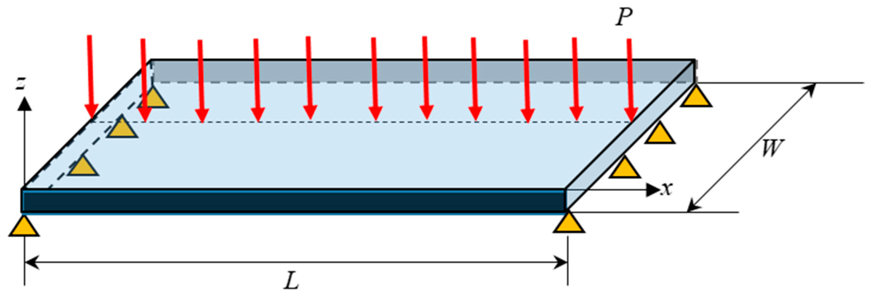
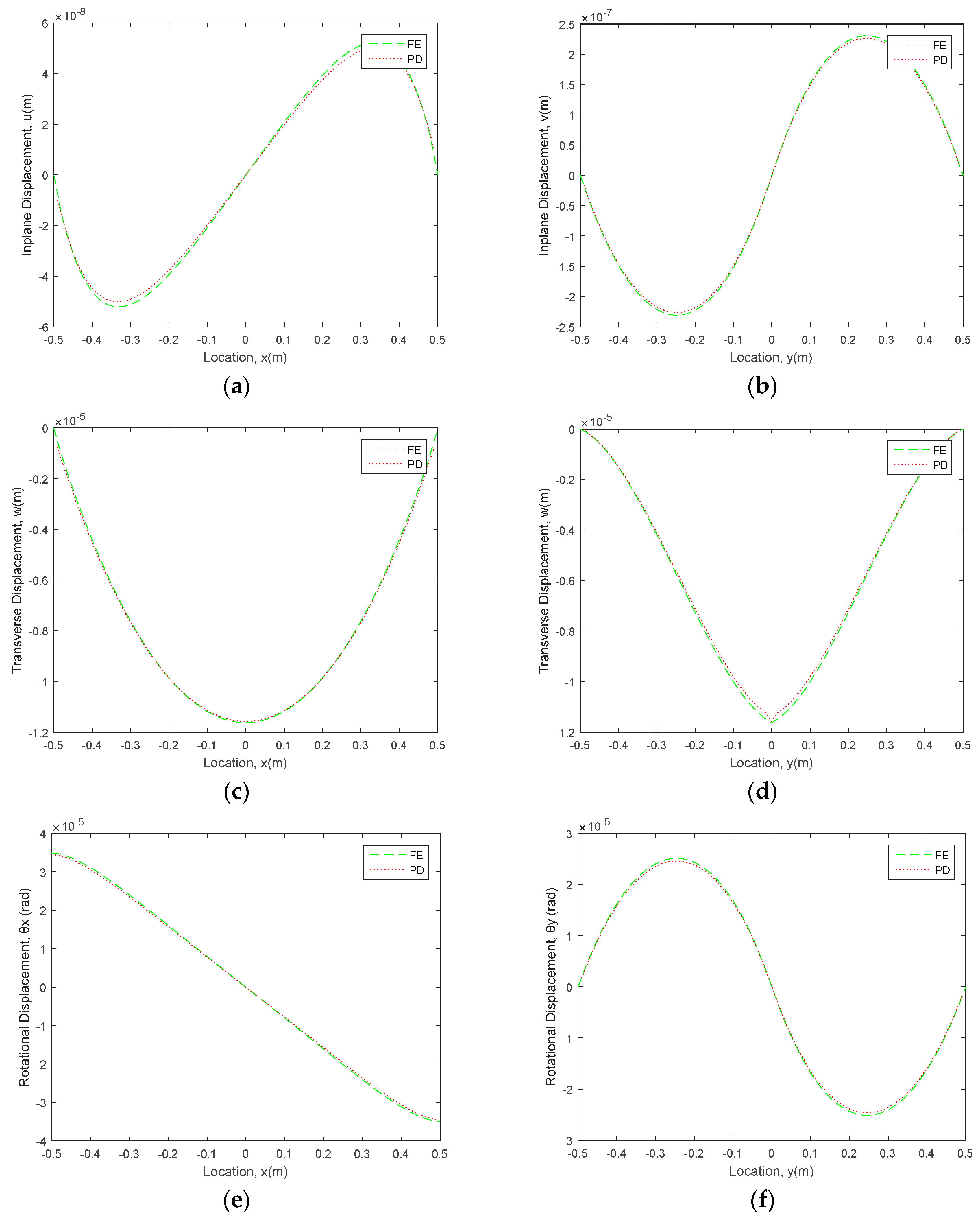
4.1. Simply Supported Functionally Graded Mindlin Plate

In the first example case, a simply supported functionally graded Mindlin plate subjected to a distributed load of $p=\mathrm{100,000} \mathrm{N}/\mathrm{m}$ through the central line is taken into consideration (see Figure 4). For the PD model, the load is transformed into a body load of $b_z=\frac{\mathrm{pW}}{65\Delta A}=\mathrm{6,500,000} \mathrm{N}/{\mathrm{m}}^2$ and it is imposed on a row of material points through the central line of the plate as shown in Figure 5.

Assuming the coordinate system is attached at the geometric centre of the plate, the following boundary conditions are applied in ANSYS:

$$\mathrm{u}\left(-\frac{L}{2}, y, 0\right)=\mathrm{u}\left(\frac{L}{2}, y, 0\right)=\mathrm{u}\left(x,-\frac{W}{2}, 0\right)=\mathrm{u}\left(x, \frac{W}{2}, 0\right)=0$$

(26a)

$$\mathrm{v}\left(-\frac{L}{2}, y, 0\right)=\mathrm{v}\left(\frac{L}{2}, y, 0\right)=\mathrm{v}\left(x,-\frac{W}{2}, 0\right)=\mathrm{v}\left(x, \frac{W}{2}, 0\right)=0$$

(26b)

$$\mathrm{w}\left(-\frac{L}{2}, y, 0\right)=\mathrm{w}\left(\frac{L}{2}, y, 0\right)=\mathrm{w}\left(x,-\frac{W}{2}, 0\right)=\mathrm{w}\left(x, \frac{W}{2}, 0\right)=0$$

(26c)

$${\theta }_y\left(-\frac{L}{2}, y, 0\right)={\theta }_y\left(\frac{L}{2}, y, 0\right)=0$$

(26d)

$${\theta }_x\left(x,-\frac{W}{2}, 0\right)={\theta }_x\left(x, \frac{W}{2}, 0\right)=0$$

(26e)

The PD results for in-plane and transverse displacements, and rotations are obtained and compared with FEA results for the material points located along central x- and y- axes. As depicted in Figure 6, PD and FEA results agree very well with each other.

4.2. Fully Clamped Functionally Graded Mindlin Plate

In the second example case, the functionally graded Mindlin plate considered in the previous example is subjected to fully clamped boundary condition (see Figure 7). In ANSYS, the clamped boundary condition is achieved by constraining all degrees of freedom along the external boundaries.

Based on the comparison between the PD and FEA results as shown in Figure 8, it can be concluded that current PD formulation can also provide accurate results for fully clamped boundary condition.

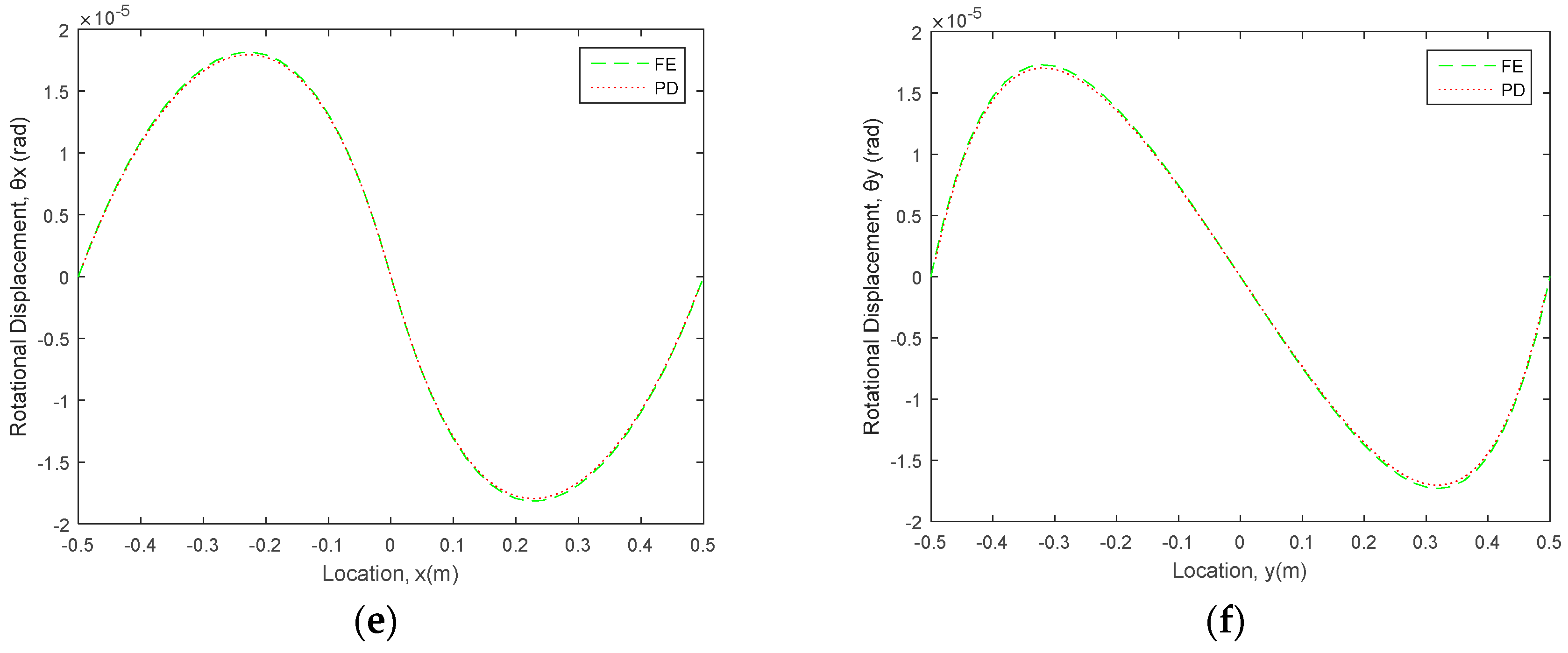
4.3. Functionally Graded Mindlin Plate Subjected to Mixed Boundary Conditions

The last numerical case aims to verify the current PD formulation for mixed boundary conditions, i.e., clamped—simply supported. As shown in Figure 9, edges along the horizontal direction are subjected to clamped boundary conditions whereas the remaining two edges are subjected to simply supported boundary conditions.

Assuming the coordinate system is attached at the geometric centre of the plate, the following boundary conditions are applied in ANSYS:

$$\mathrm{u}\left(-\frac{L}{2}, y, 0\right)=\mathrm{u}\left(\frac{L}{2}, y, 0\right)=\mathrm{u}\left(x,-\frac{W}{2}, 0\right)=\mathrm{u}\left(x, \frac{W}{2}, 0\right)=0$$

(27a)

$$\mathrm{v}\left(-\frac{L}{2}, y, 0\right)=\mathrm{v}\left(\frac{L}{2}, y, 0\right)=\mathrm{v}\left(x,-\frac{W}{2}, 0\right)=\mathrm{v}\left(x, \frac{W}{2}, 0\right)=0$$

(27b)

$$\mathrm{w}\left(-\frac{L}{2}, y, 0\right)=\mathrm{w}\left(\frac{L}{2}, y, 0\right)=\mathrm{w}\left(x,-\frac{W}{2}, 0\right)=\mathrm{w}\left(x, \frac{W}{2}, 0\right)=0$$

(27c)

$${\theta }_x\left(-\frac{L}{2}, y, 0\right)={\theta }_x\left(\frac{L}{2}, y, 0\right)={\theta }_x\left(x,-\frac{W}{2}, 0\right)={\theta }_x\left(x, \frac{W}{2}, 0\right)=0$$

(27d)

$${\theta }_y\left(-\frac{L}{2}, y, 0\right)={\theta }_y\left(\frac{L}{2}, y, 0\right)=0$$

(27e)

As depicted in Figure 10, also for this mixed-boundary conditions case, PD and FEM results agree well with each other.

5. Conclusions

In this study, a new peridynamic formulation was presented for functionally graded Mindlin plates. The governing equations were obtained by using Euler-Lagrange equations. To validate the formulation, three different benchmark problems were considered for simply supported, fully clamped and mixed (clamped-simply supported) boundary conditions. Peridynamic results were compared against finite element analysis results and a good agreement is observed for both in-plane and transverse displacements, and rotations. Hence, it can be concluded that the present peridynamic formulation can be a suitable alternative for the analysis of functionally graded Mindlin plates subjected to different types of boundary conditions.

References

1. Vel, S.; Batra, R.C. Three-dimensional exact solution for the vibration of functionally graded rectangular plates. J. Sound Vib. 2004, 272, 703–730. [Google Scholar] [CrossRef]
2. Shen, H.-S. Nonlinear bending response of functionally graded plates subjected to transverse loads and in thermal environments. Int. J. Mech. Sci. 2002, 44, 561–584. [Google Scholar] [CrossRef]
3. Zenkour, A. Generalized shear deformation theory for bending analysis of functionally graded plates. Appl. Math. Model. 2006, 30, 67–84. [Google Scholar] [CrossRef] [Green Version]
4. Bian, Z.; Chen, W.; Lim, C.W.; Zhang, N. Analytical solutions for single- and multi-span functionally graded plates in cylindrical bending. Int. J. Solids Struct. 2005, 42, 6433–6456. [Google Scholar] [CrossRef] [Green Version]
5. Carrera, E.; Brischetto, S.; Cinefra, M.; Soave, M. Effects of thickness stretching in functionally graded plates and shells. Compos. Part B Eng. 2011, 42, 123–133. [Google Scholar] [CrossRef] [Green Version]
6. Ferreira, A.; Batra, R.C.; Roque, C.; Qian, L.; Martins, P. Static analysis of functionally graded plates using third-order shear deformation theory and a meshless method. Compos. Struct. 2005, 69, 449–457. [Google Scholar] [CrossRef]
7. Kashtalyan, M. Three-dimensional elasticity solution for bending of functionally graded rectangular plates. Eur. J. Mech. A Solids 2004, 23, 853–864. [Google Scholar] [CrossRef]
8. Xiang, S.; Kang, G.-W. A nth-order shear deformation theory for the bending analysis on the functionally graded plates. Eur. J. Mech. A Solids 2013, 37, 336–343. [Google Scholar] [CrossRef]
9. Silling, S. Reformulation of elasticity theory for discontinuities and long-range forces. J. Mech. Phys. Solids 2000, 48, 175–209. [Google Scholar] [CrossRef] [Green Version]
10. Silling, S.A.; Epton, M.; Weckner, O.; Xu, J.; Askari, E. Peridynamic States and Constitutive Modeling. J. Elast. 2007, 88, 151–184. [Google Scholar] [CrossRef] [Green Version]
11. Jenabidehkordi, A.; Rabczuk, T.; Ma, B.; Dui, G.; Yang, S.; Xin, L. The Multi-Horizon Peridynamics. Comput. Model. Eng. Sci. 2019, 121, 493–500. [Google Scholar] [CrossRef] [Green Version]
12. Wang, X.; Kulkarni, S.S.; Tabarraei, A. Concurrent coupling of peridynamics and classical elasticity for elastodynamic problems. Comput. Methods Appl. Mech. Eng. 2019, 344, 251–275. [Google Scholar] [CrossRef]
13. Ni, T.; Zaccariotto, M.; Zhu, Q.-Z.; Galvanetto, U. Static solution of crack propagation problems in Peridynamics. Comput. Methods Appl. Mech. Eng. 2019, 346, 126–151. [Google Scholar] [CrossRef]
14. Chowdhury, S.R.; Roy, P.; Roy, D.; Reddy, J.N. A modified peridynamics correspondence principle: Removal of zero-energy deformation and other implications. Comput. Methods Appl. Mech. Eng. 2019, 346, 530–549. [Google Scholar] [CrossRef]
15. Liu, S.; Fang, G.; Liang, J.; Fu, M.; Wang, B. A new type of peridynamics: Element-based peridynamics. Comput. Methods Appl. Mech. Eng. 2020, 366, 113098. [Google Scholar] [CrossRef]
16. Diehl, P.; Prudhomme, S.; Lévesque, M. A Review of Benchmark Experiments for the Validation of Peridynamics Models. J. Peridynamics Nonlocal Model. 2019, 1, 14–35. [Google Scholar] [CrossRef]
17. Katiyar, A.; Agrawal, S.; Ouchi, H.; Seleson, P.; Foster, J.T.; Sharma, M.M. A general peridynamics model for multiphase transport of non-Newtonian compressible fluids in porous media. J. Comput. Phys. 2020, 402, 109075. [Google Scholar] [CrossRef]
18. Song, X.; Khalili, N. A peridynamics model for strain localization analysis of geomaterials. Int. J. Numer. Anal. Methods Géoméch. 2018, 43, 77–96. [Google Scholar] [CrossRef] [Green Version]
19. Ozdemir, M.; Kefal, A.; Imachi, M.; Tanaka, S.; Oterkus, E. Dynamic fracture analysis of functionally graded materials using ordinary state-based peridynamics. Compos. Struct. 2020, 244, 112296. [Google Scholar] [CrossRef]
20. Oterkus, E.; Madenci, E. Peridynamics for failure prediction in composites. In Proceedings of the 53rd AIAA/ASME/ASCE/AHS/ASC Structures, Structural Dynamics and Materials Conference 20th AIAA/ASME/AHS Adaptive Structures Conference 14th AIAA, Honolulu, HI, USA, 23–26 April 2012; p. 1692. [Google Scholar]
21. Yang, Z.; Oterkus, E.; Nguyen, C.T.; Oterkus, S. Implementation of peridynamic beam and plate formulations in finite element framework. Contin. Mech. Thermodyn. 2018, 31, 301–315. [Google Scholar] [CrossRef] [Green Version]
22. Diyaroglu, C.; Oterkus, S.; Oterkus, E.; Madenci, E. Peridynamic Modeling of Diffusion by Using Finite-Element Analysis. IEEE Trans. Components Packag. Manuf. Technol. 2017, 7, 1–9. [Google Scholar] [CrossRef] [Green Version]
23. Zhu, N.; De Meo, D.; Oterkus, E. Modelling of Granular Fracture in Polycrystalline Materials Using Ordinary State-Based Peridynamics. Materials 2016, 9, 977. [Google Scholar] [CrossRef] [PubMed] [Green Version]
24. Imachi, M.; Tanaka, S.; Bui, T.Q.; Oterkus, S.; Oterkus, E. A computational approach based on ordinary state-based peridynamics with new transition bond for dynamic fracture analysis. Eng. Fract. Mech. 2019, 206, 359–374. [Google Scholar] [CrossRef] [Green Version]
25. Gao, Y.; Oterkus, S. Ordinary state-based peridynamic modelling for fully coupled thermoelastic problems. Contin. Mech. Thermodyn. 2018, 31, 907–937. [Google Scholar] [CrossRef] [Green Version]
26. Wang, H.; Oterkus, E.; Oterkus, S. Predicting fracture evolution during lithiation process using peridynamics. Eng. Fract. Mech. 2018, 192, 176–191. [Google Scholar] [CrossRef] [Green Version]
27. Alpay, S.; Madenci, E. Crack growth prediction in fully-coupled thermal and deformation fields using peridynamic theory. In Proceedings of the 54th AIAA/ASME/ASCE/AHS/ASC Structures, Structural Dynamics, and Materials Conference, Boston, MA, USA, 8–11 April 2013; p. 1477. [Google Scholar]
28. Diyaroglu, C.; Oterkus, E.; Oterkus, S. An Euler–Bernoulli beam formulation in an ordinary state-based peridynamic framework. Math. Mech. Solids 2017, 24, 361–376. [Google Scholar] [CrossRef]
29. Zhao, J.; Chen, Z.; Mehrmashhadi, J.; Bobaru, F. A stochastic multiscale peridynamic model for corrosion-induced fracture in reinforced concrete. Eng. Fract. Mech. 2020, 229, 106969. [Google Scholar] [CrossRef] [Green Version]
30. De Meo, D.; Diyaroglu, C.; Zhu, N.; Oterkus, E.; Siddiq, M.A. Modelling of stress-corrosion cracking by using peridynamics. Int. J. Hydrogen Energy 2016, 41, 6593–6609. [Google Scholar] [CrossRef] [Green Version]
31. Ghajari, M.; Iannucci, L.; Curtis, P. A peridynamic material model for the analysis of dynamic crack propagation in orthotropic media. Comput. Methods Appl. Mech. Eng. 2014, 276, 431–452. [Google Scholar] [CrossRef] [Green Version]
32. Cheng, Z.; Zhang, G.; Wang, Y.; Bobaru, F. A peridynamic model for dynamic fracture in functionally graded materials. Compos. Struct. 2015, 133, 529–546. [Google Scholar] [CrossRef]
33. Oterkus, E.; Guven, I.; Madenci, E. Impact damage assessment by using peridynamic theory. Open Eng. 2012, 2, 523–531. [Google Scholar] [CrossRef]
34. Liu, X.; He, X.; Wang, J.; Sun, L.G.; Oterkus, E. An ordinary state-based peridynamic model for the fracture of zigzag graphene sheets. Proc. R. Soc. A Math. Phys. Eng. Sci. 2018, 474, 20180019. [Google Scholar] [CrossRef] [PubMed] [Green Version]
35. Madenci, E.; Oterkus, S. Ordinary state-based peridynamics for plastic deformation according to von Mises yield criteria with isotropic hardening. J. Mech. Phys. Solids 2016, 86, 192–219. [Google Scholar] [CrossRef] [Green Version]
36. Weckner, O.; Mohamed, N.A.N. Viscoelastic material models in peridynamics. Appl. Math. Comput. 2013, 219, 6039–6043. [Google Scholar] [CrossRef]
37. Foster, J.T.; Silling, S.A.; Chen, W.W. Viscoplasticity using peridynamics. Int. J. Numer. Methods Eng. 2009, 81, 1242–1258. [Google Scholar] [CrossRef]
38. Oterkus, S.; Madenci, E.; Agwai, A. Peridynamic thermal diffusion. J. Comput. Phys. 2014, 265, 71–96. [Google Scholar] [CrossRef] [Green Version]
39. Diyaroglu, C.; Oterkus, S.; Oterkus, E.; Madenci, E.; Han, S.; Hwang, Y. Peridynamic wetness approach for moisture concentration analysis in electronic packages. Microelectron. Reliab. 2017, 70, 103–111. [Google Scholar] [CrossRef] [Green Version]
40. Ouchi, H.; Katiyar, A.; York, J.; Foster, J.; Sharma, M.M. A fully coupled porous flow and geomechanics model for fluid driven cracks: A peridynamics approach. Comput. Mech. 2015, 55, 561–576. [Google Scholar] [CrossRef]
41. Taylor, M.; Steigmann, D. A two-dimensional peridynamic model for thin plates. Math. Mech. Solids 2013, 20, 998–1010. [Google Scholar] [CrossRef]
42. O’Grady, J.; Foster, J. Peridynamic beams: A non-ordinary, state-based model. Int. J. Solids Struct. 2014, 51, 3177–3183. [Google Scholar] [CrossRef] [Green Version]
43. O’Grady, J.; Foster, J. Peridynamic plates and flat shells: A non-ordinary, state-based model. Int. J. Solids Struct. 2014, 51, 4572–4579. [Google Scholar] [CrossRef] [Green Version]
44. Diyaroglu, C.; Oterkus, E.; Oterkus, S.; Madenci, E. Peridynamics for bending of beams and plates with transverse shear deformation. Int. J. Solids Struct. 2015, 69, 152–168. [Google Scholar] [CrossRef] [Green Version]
45. Chowdhury, S.R.; Roy, P.; Roy, D.; Reddy, J.N. A peridynamic theory for linear elastic shells. Int. J. Solids Struct. 2016, 84, 110–132. [Google Scholar] [CrossRef]
46. Madenci, E.; Oterkus, E. Peridynamic Theory and Its Applications; Springer: New York, NY, USA, 2014; Volume 17. [Google Scholar]
47. Javili, A.; Morasata, R.; Oterkus, E.; Oterkus, S. Peridynamics review. Math. Mech. Solids 2018, 24, 3714–3739. [Google Scholar] [CrossRef] [Green Version]
Figure 1. The positive set of the degrees-of-freedom for Mindlin plate formulation.
Jcs 04 00076 g001
Figure 2. Peridynamics (PD) force density vector and horizon [46].
Jcs 04 00076 g002
Figure 3. Variation of material properties through the thickness direction for the finite element model.
Jcs 04 00076 g003
Figure 4. Simply supported functionally graded Mindlin plate.
Jcs 04 00076 g004
Figure 5. Numerical discretization, loading and fictitious region.
Jcs 04 00076 g005
Figure 6. Comparison of PD and FEA results along the central x- and y-axes.
Jcs 04 00076 g006
Figure 7. Fully clamped functionally graded Mindlin plate.
Jcs 04 00076 g007
Figure 8. Comparison of PD and FEA results along the central x- and y-axes.
Jcs 04 00076 g008aJcs 04 00076 g008b
Figure 9. Functionally graded Mindlin plate subjected to mixed boundary conditions.
Jcs 04 00076 g009
Figure 10. Comparison of PD and FEA results along the central x- and y-axes.
Jcs 04 00076 g010