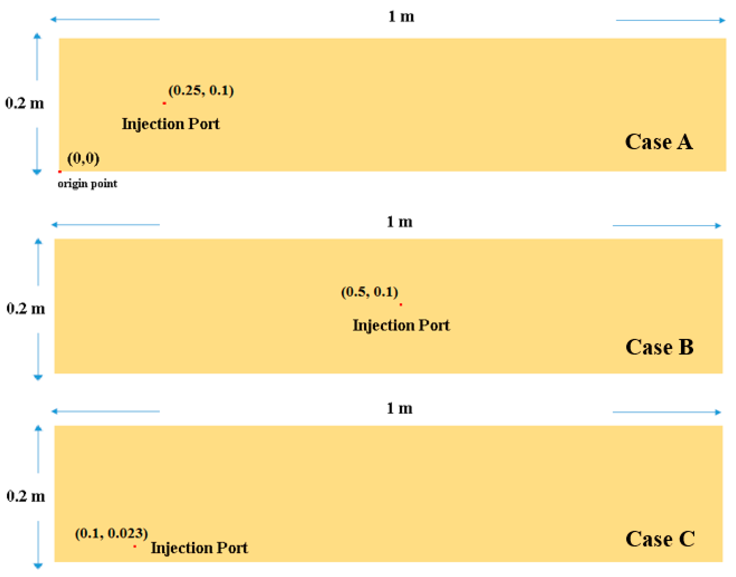
Figure 1.
Selected cases with different injection port positions: case A (top picture), case B (middle picture) and case C (bottom picture). The coordinates of the points are given in meters with respect to the origin point.
Figure 1.
Selected cases with different injection port positions: case A (top picture), case B (middle picture) and case C (bottom picture). The coordinates of the points are given in meters with respect to the origin point.
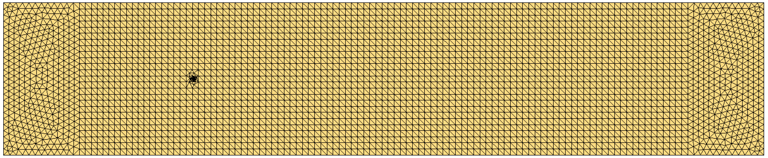
Figure 2.
Finite element mesh used for case A in
Figure 1.
Figure 2.
Finite element mesh used for case A in
Figure 1.
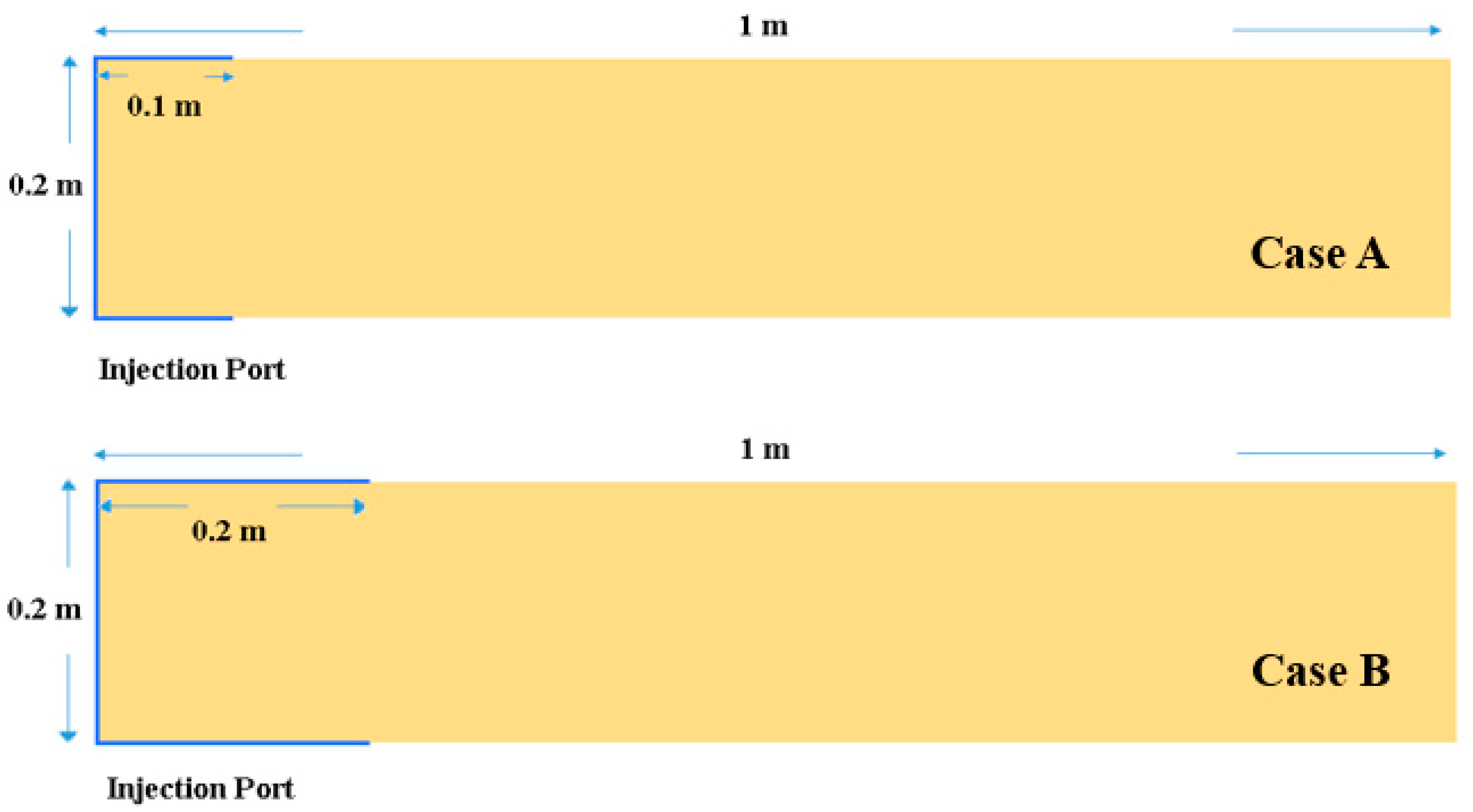
Figure 3.
Selected cases of injection through a C-shaped inlet: case A (top picture) and case B (bottom picture).
Figure 3.
Selected cases of injection through a C-shaped inlet: case A (top picture) and case B (bottom picture).
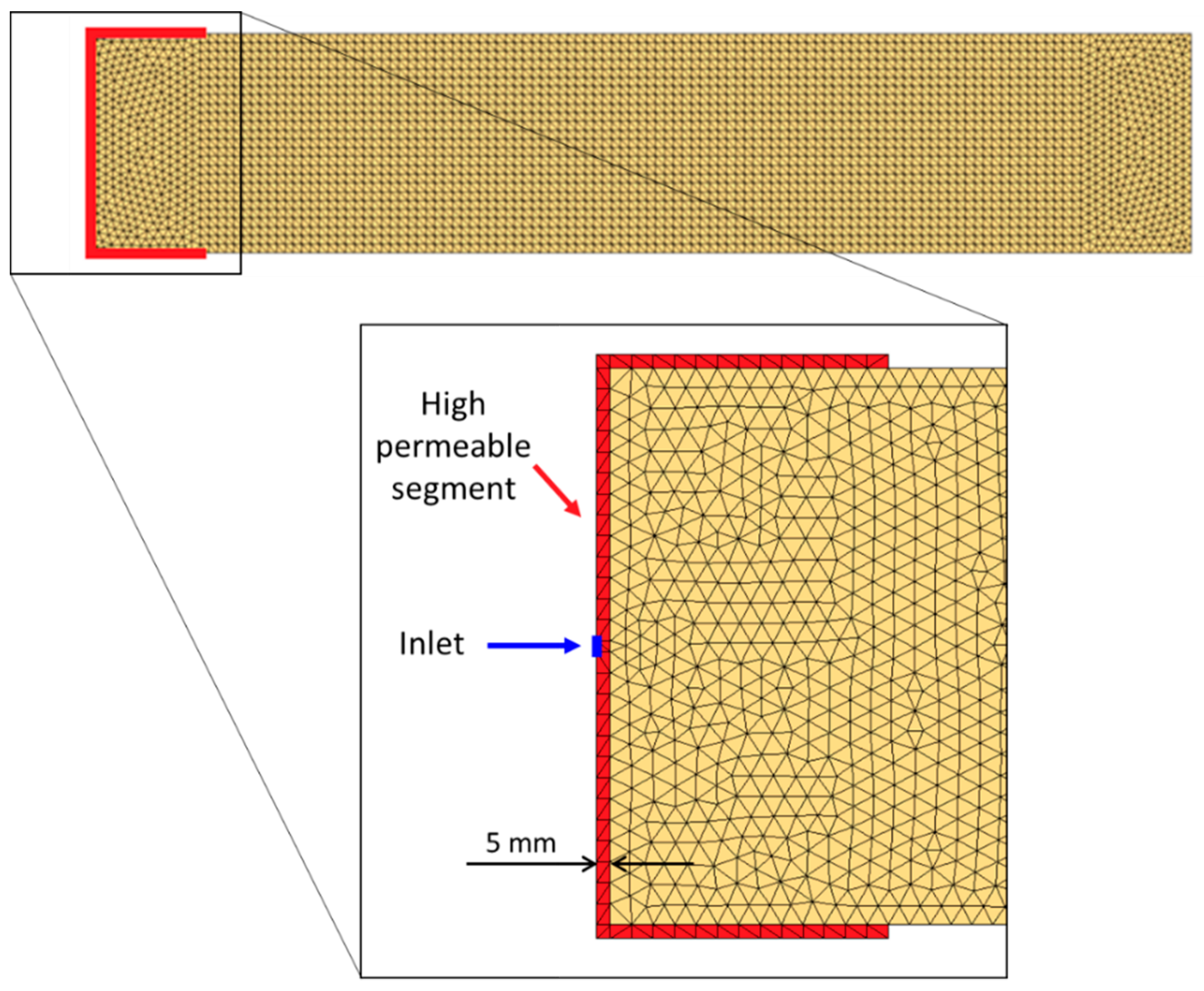
Figure 4.
Design of C-shaped inlet used for simulating case A in
Figure 3.
Figure 4.
Design of C-shaped inlet used for simulating case A in
Figure 3.
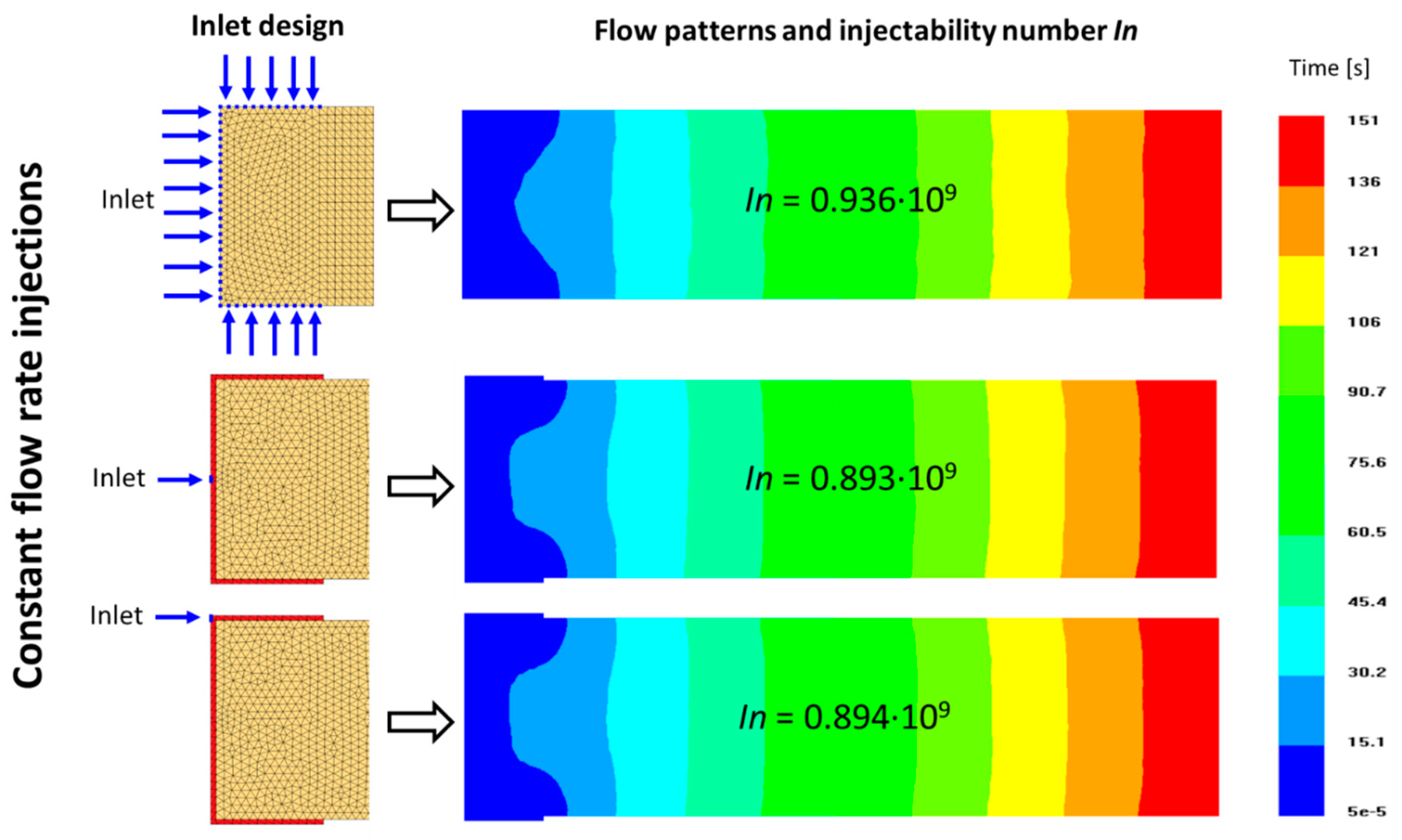
Figure 5.
Comparison of flow patterns and injectability numbers obtained in constant flow rate injections for different designs of the C-shaped inlet.
Figure 5.
Comparison of flow patterns and injectability numbers obtained in constant flow rate injections for different designs of the C-shaped inlet.
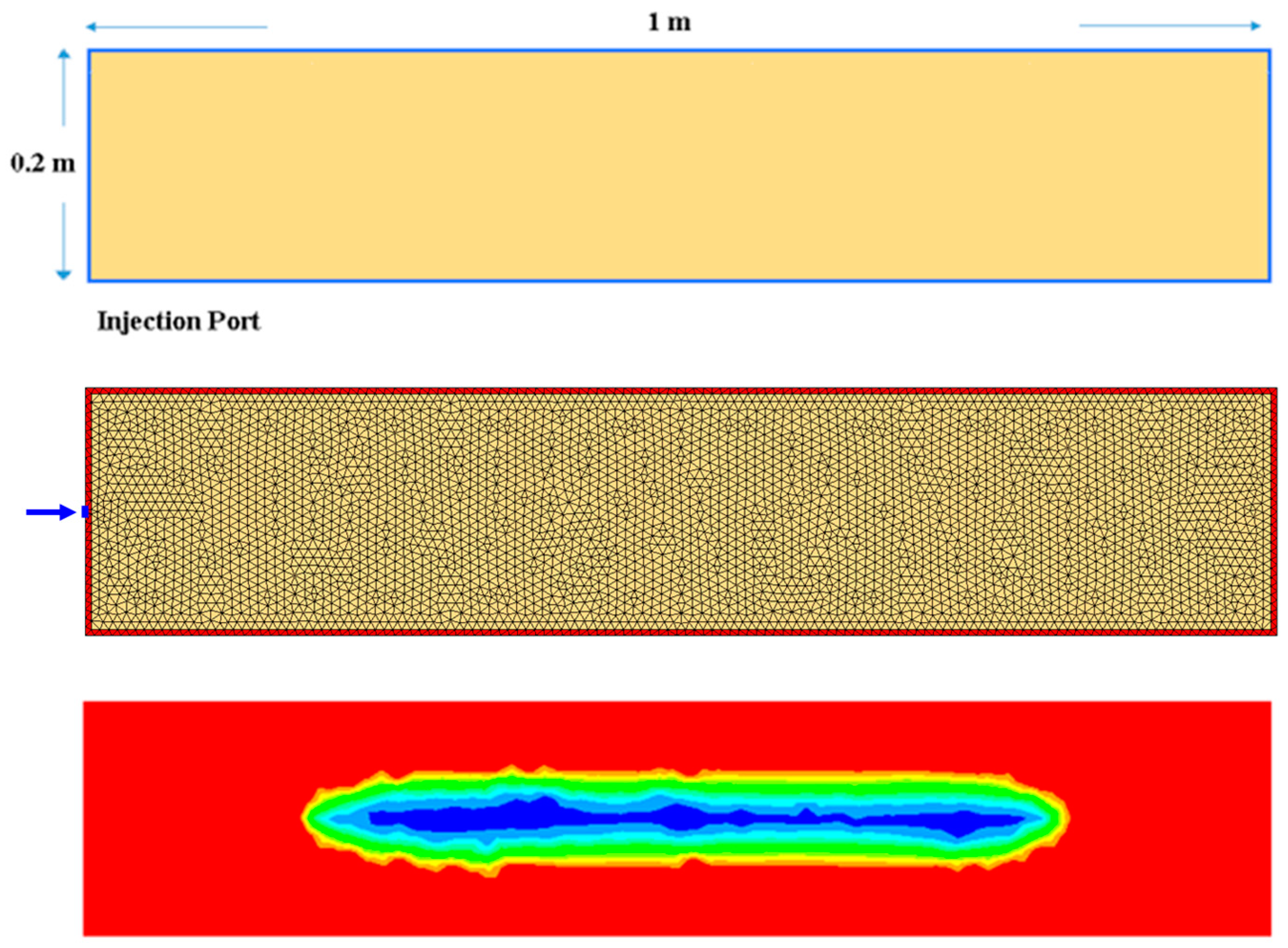
Figure 6.
Peripheral injection case: geometry (top picture), mesh with surrounding high permeable segments (middle picture) and filling pattern with air entrapment (bottom picture).
Figure 6.
Peripheral injection case: geometry (top picture), mesh with surrounding high permeable segments (middle picture) and filling pattern with air entrapment (bottom picture).
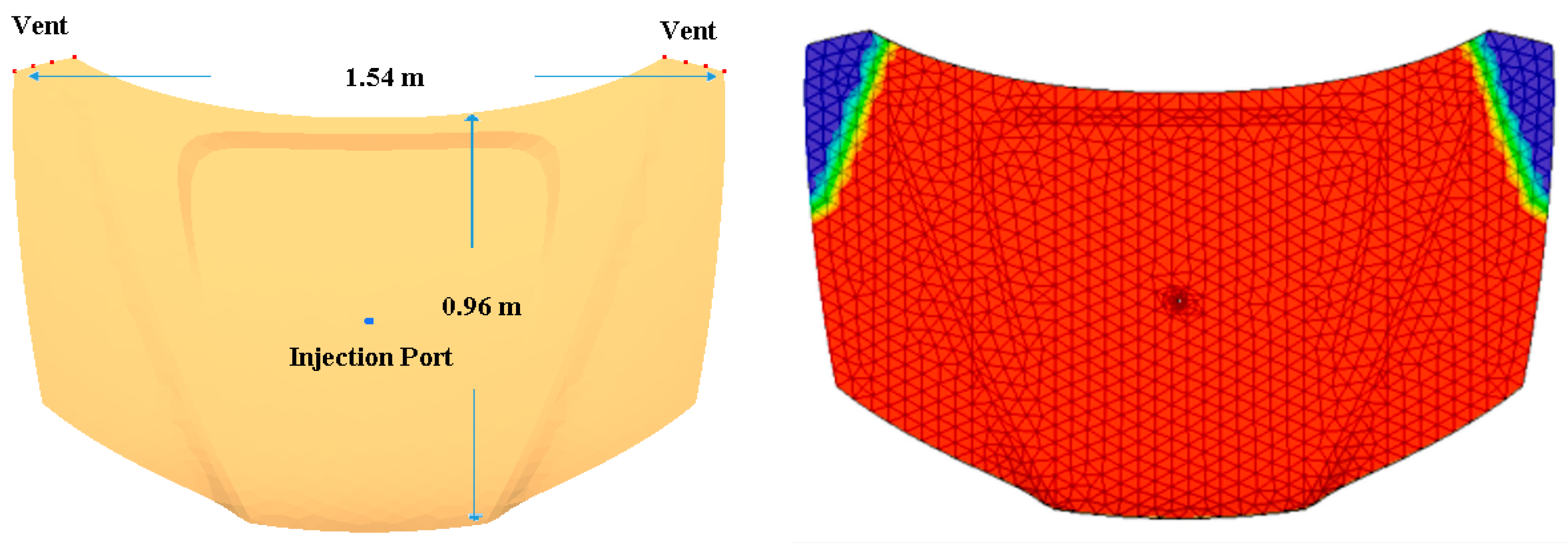
Figure 7.
First geometry (top picture) and injection simulation (bottom picture) of composite vehicle hood (distances are given in meters).
Figure 7.
First geometry (top picture) and injection simulation (bottom picture) of composite vehicle hood (distances are given in meters).
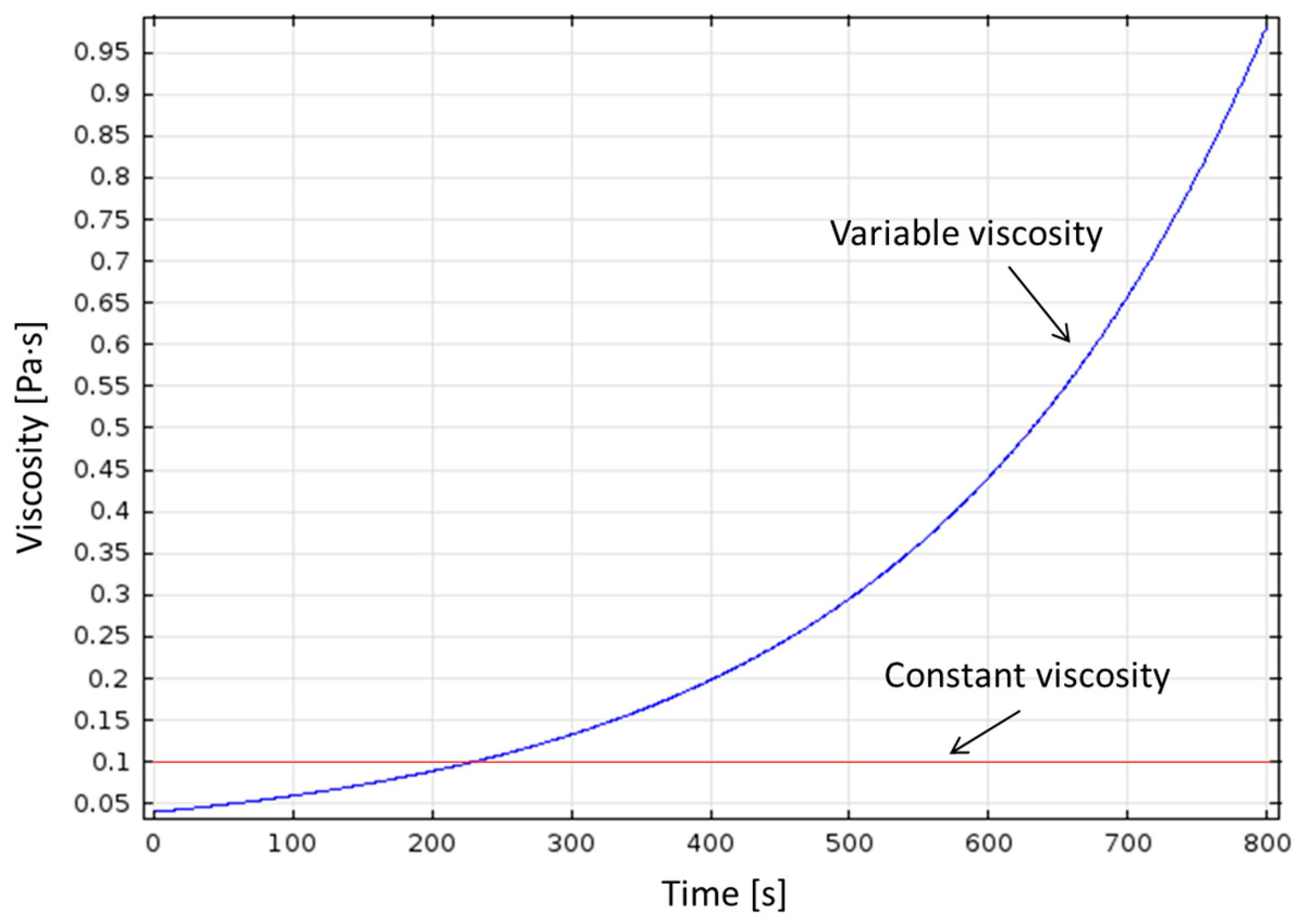
Figure 8.
Viscosity curves for the filling simulations of the first hood geometry.
Figure 8.
Viscosity curves for the filling simulations of the first hood geometry.
Figure 9.
Second geometry (left) and injection simulation (right) of composite vehicle hood.
Figure 9.
Second geometry (left) and injection simulation (right) of composite vehicle hood.
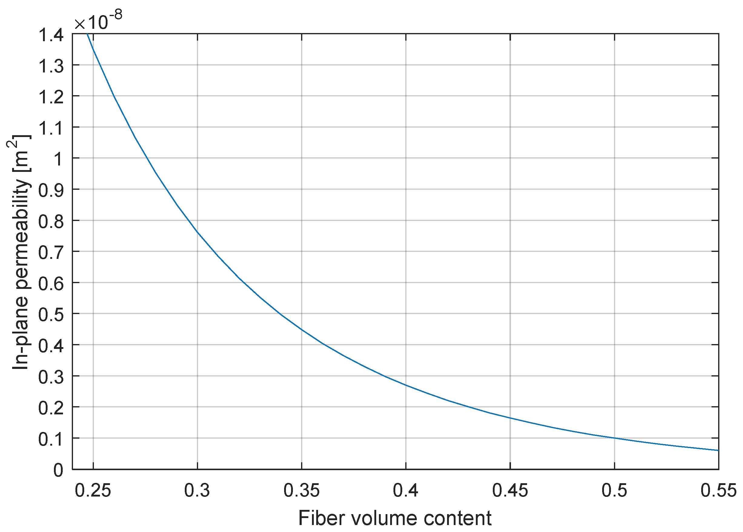
Figure 10.
In-plane permeability (K1, K2) curve for the C-RTM process simulations for the second hood geometry.
Figure 10.
In-plane permeability (K1, K2) curve for the C-RTM process simulations for the second hood geometry.
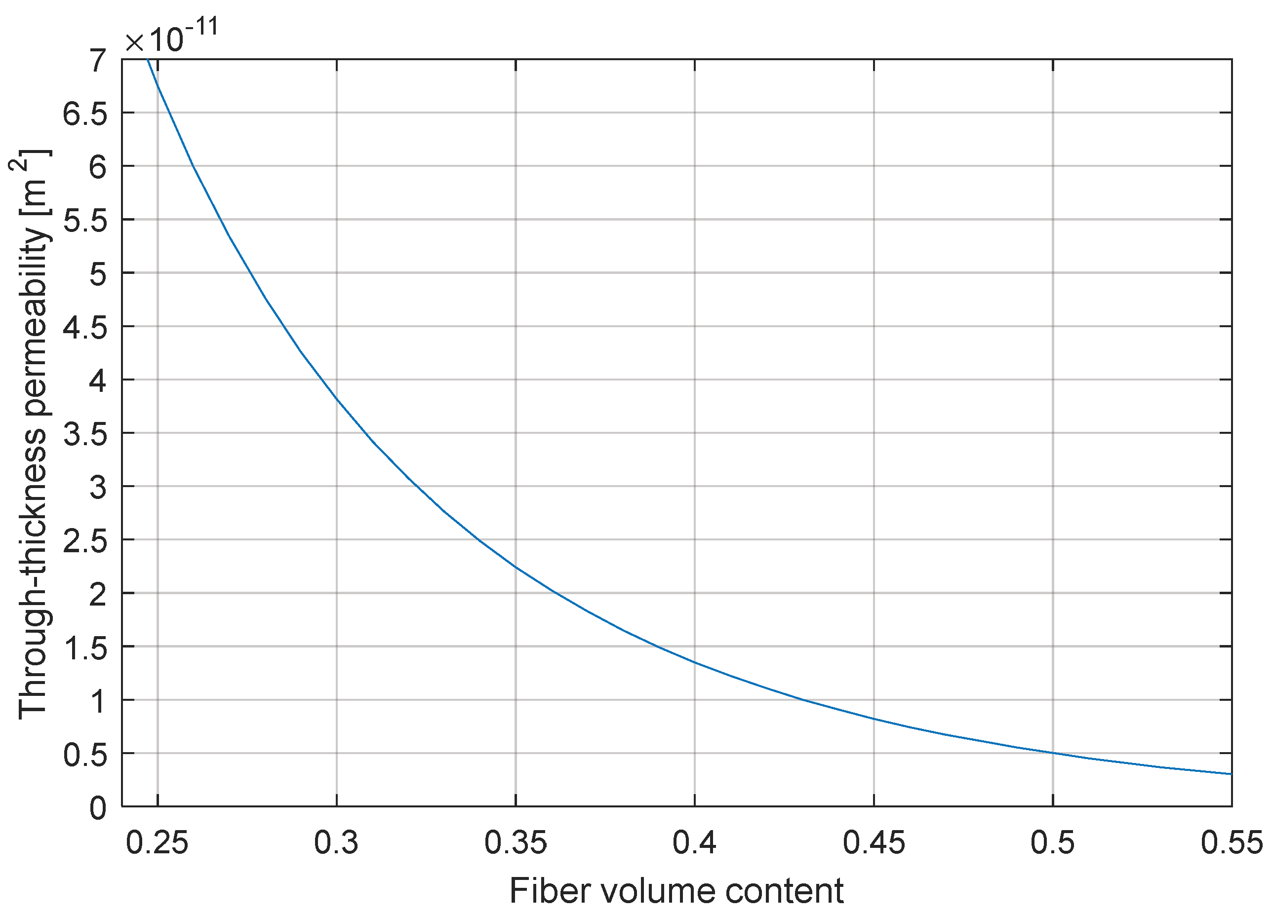
Figure 11.
Through-thickness permeability (K3) curve for the C-RTM process simulations for the second hood geometry.
Figure 11.
Through-thickness permeability (K3) curve for the C-RTM process simulations for the second hood geometry.
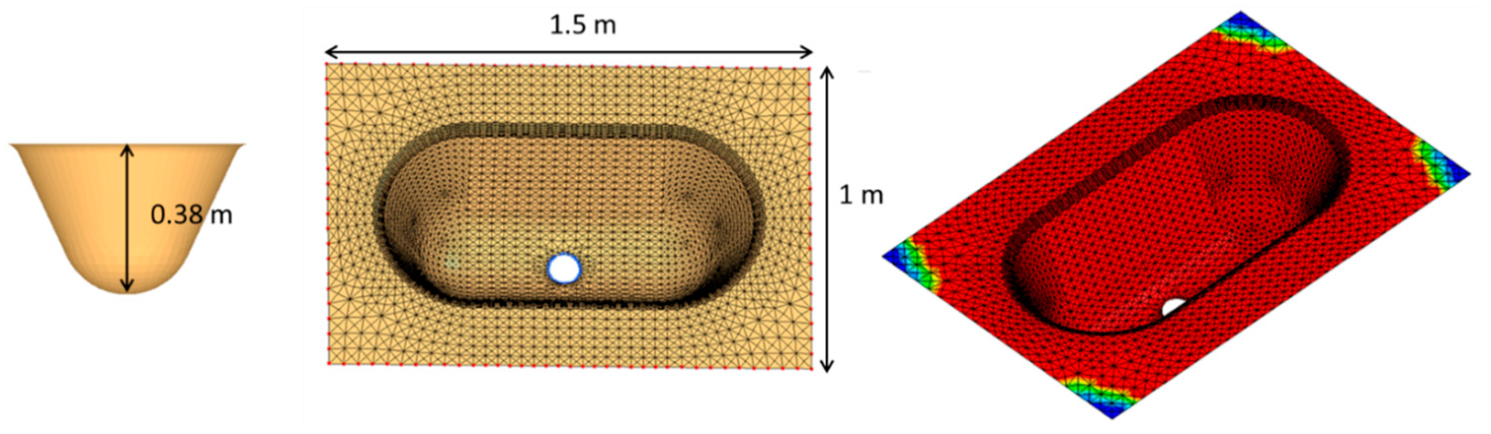
Figure 12.
Geometry, mesh and injection simulation of composite reservoir.
Figure 12.
Geometry, mesh and injection simulation of composite reservoir.
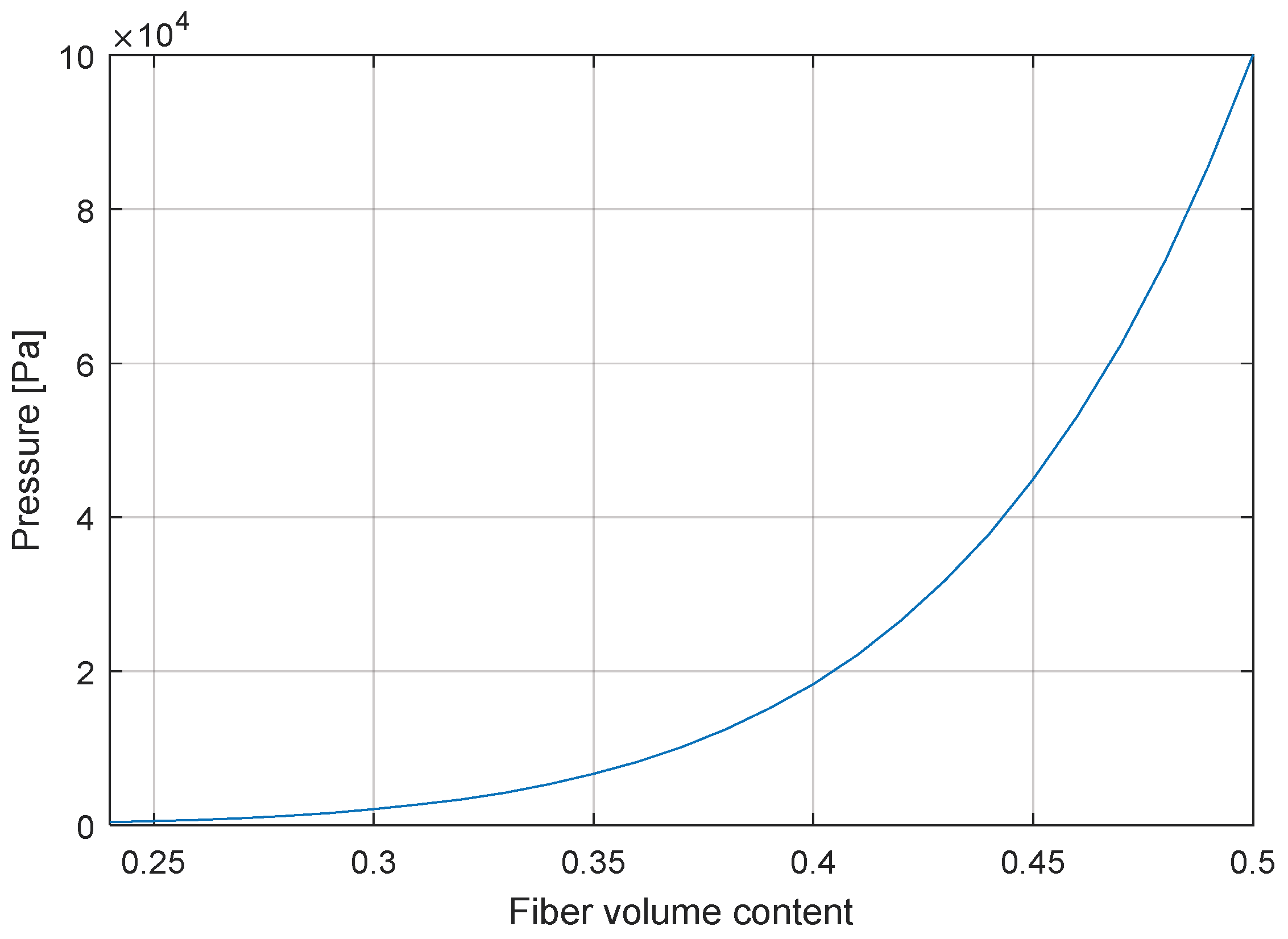
Figure 13.
Compaction curve used in VARI simulation.
Figure 13.
Compaction curve used in VARI simulation.
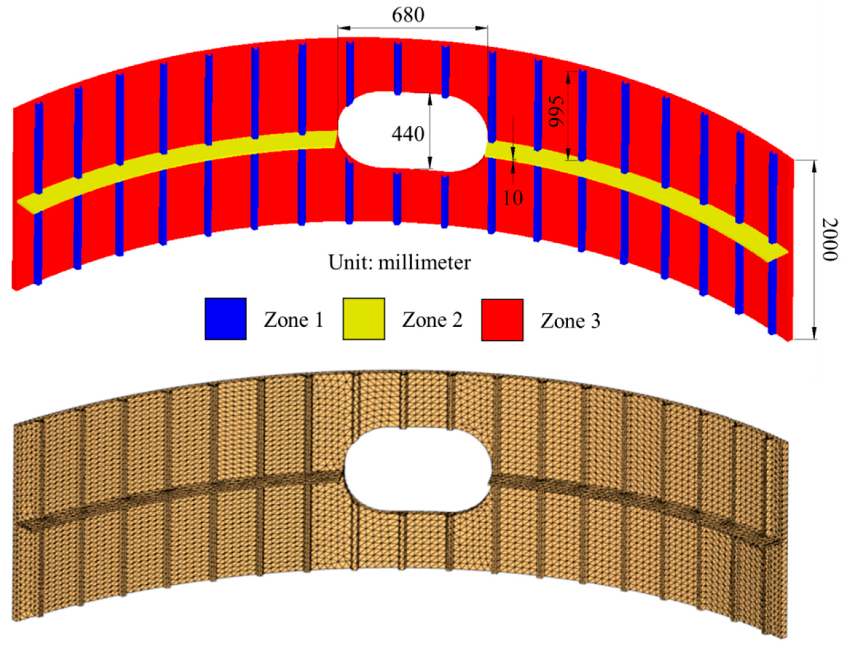
Figure 14.
Fuselage section geometry and mesh.
Figure 14.
Fuselage section geometry and mesh.
Figure 15.
Details of the fuselage section geometry.
Figure 15.
Details of the fuselage section geometry.
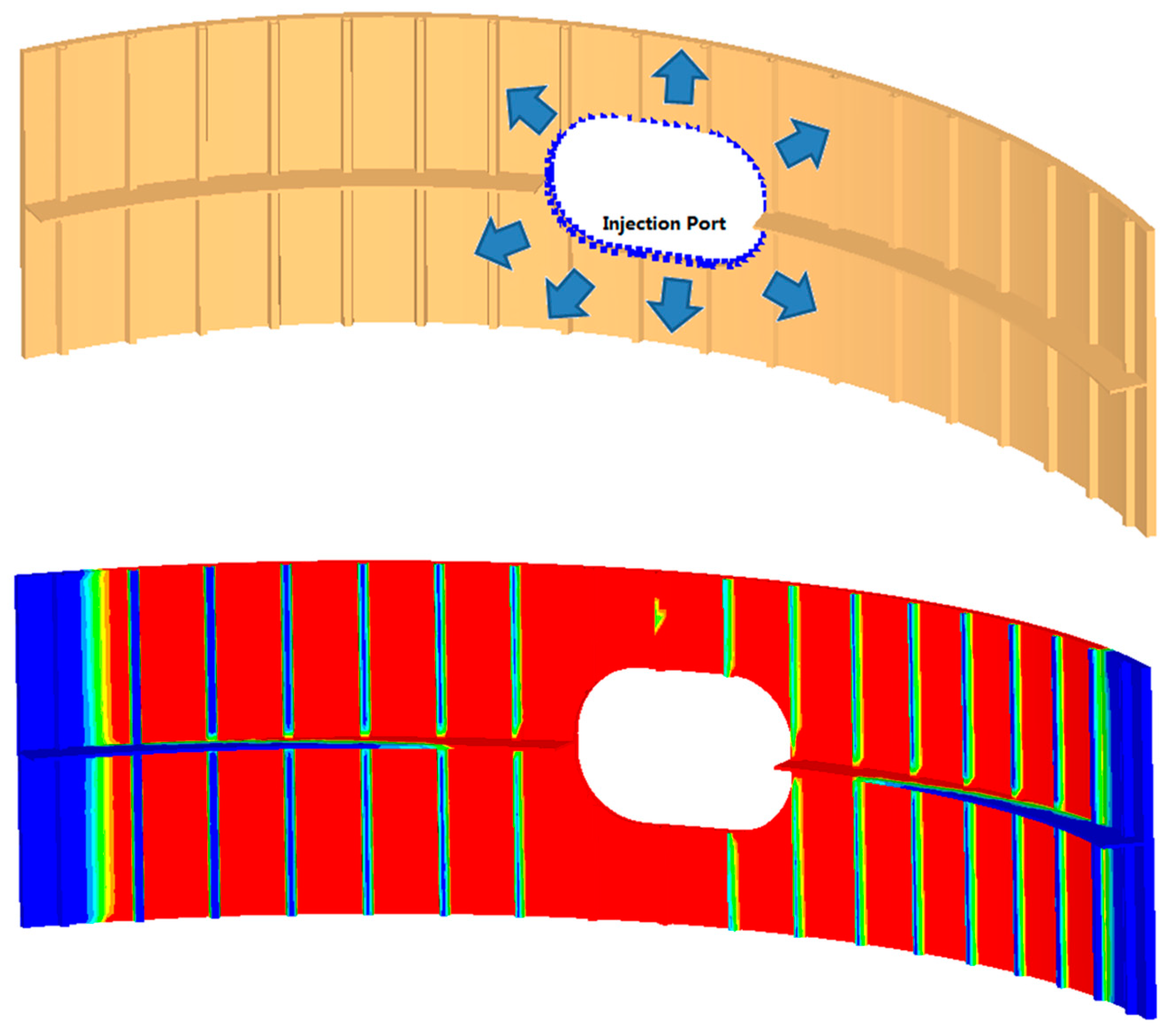
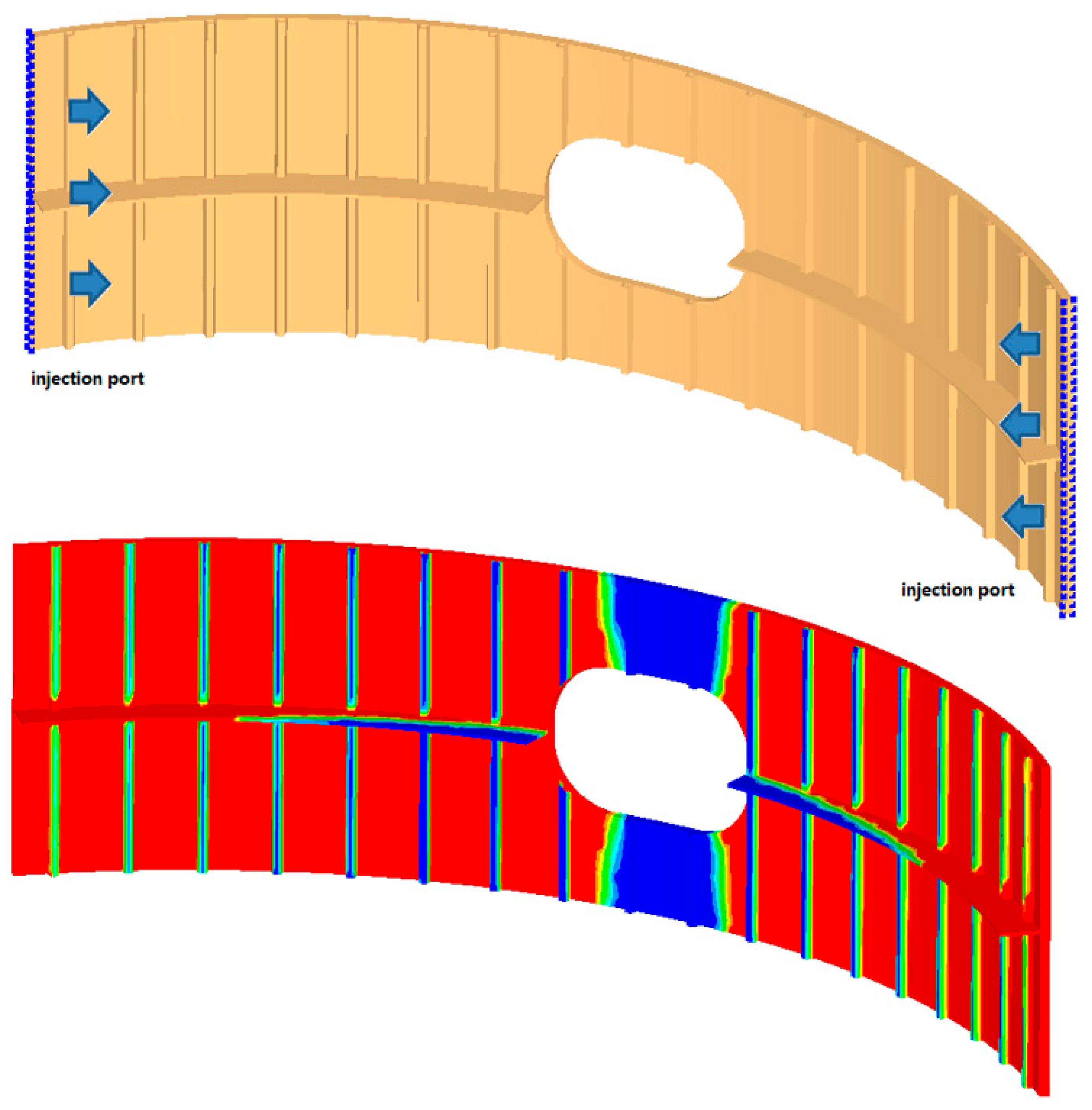
Figure 16.
Injection case A for the fuselage section.
Figure 16.
Injection case A for the fuselage section.
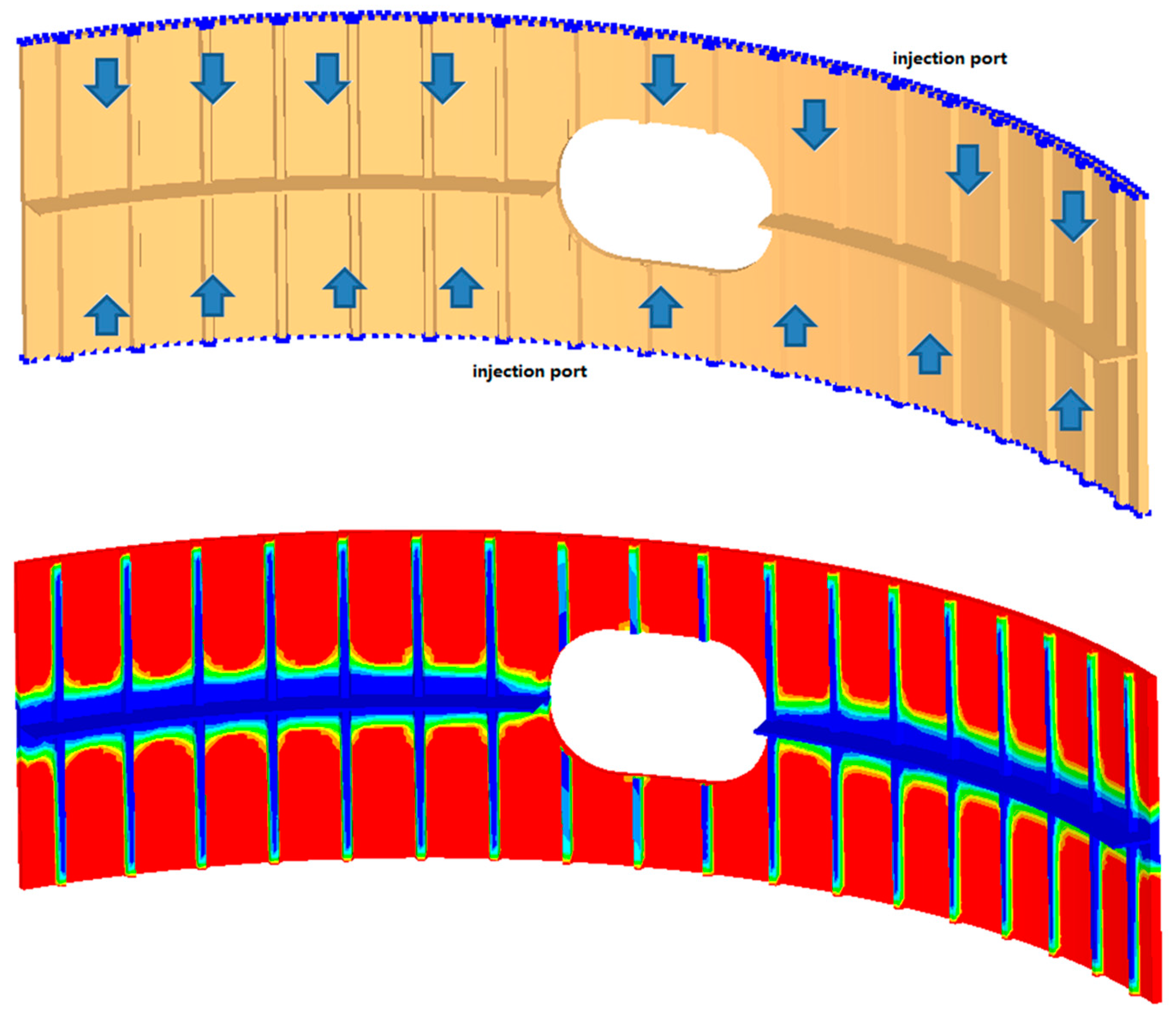
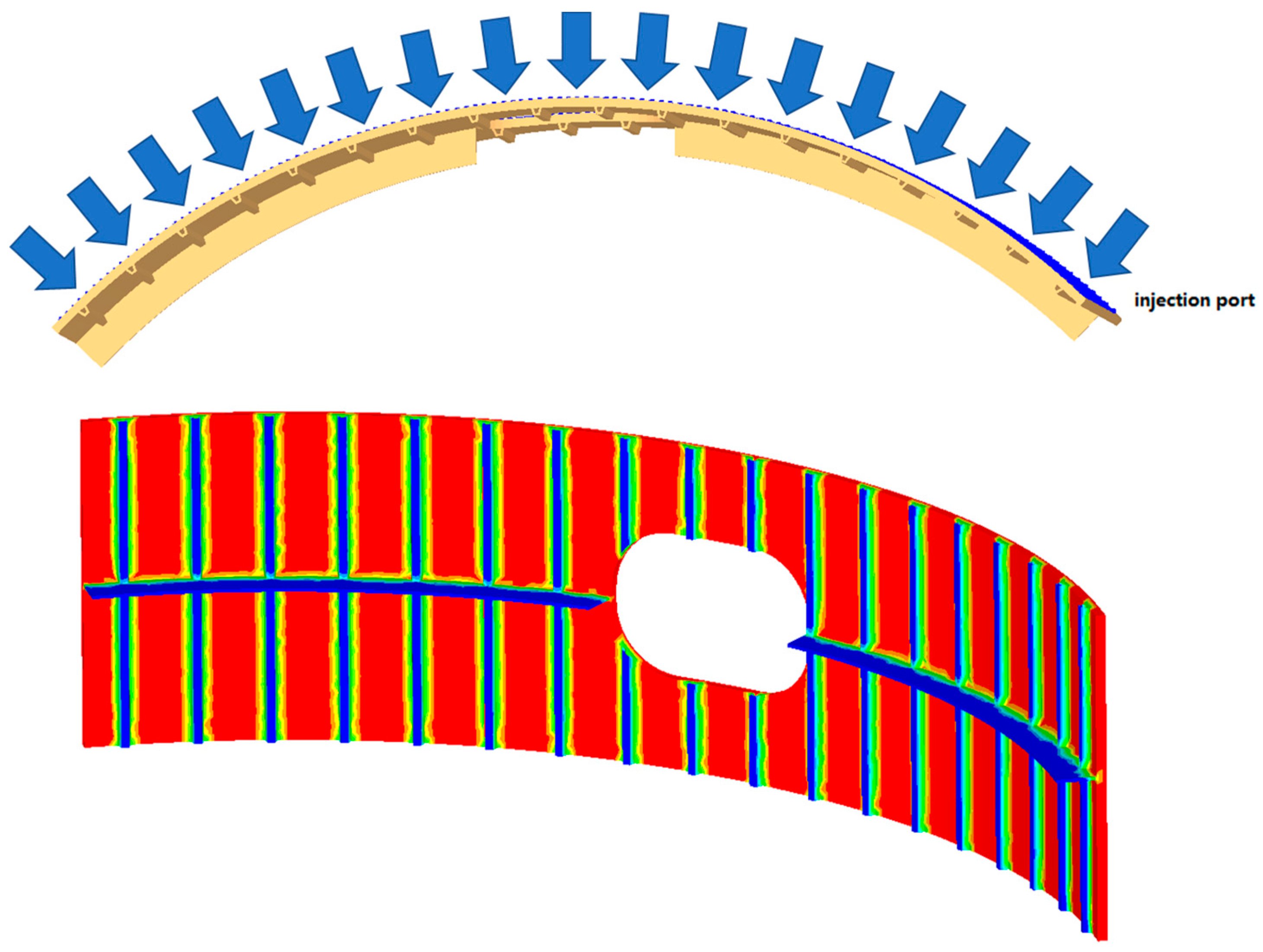
Figure 17.
Injection case B for the fuselage section.
Figure 17.
Injection case B for the fuselage section.
Figure 18.
Injection case C for the fuselage section.
Figure 18.
Injection case C for the fuselage section.
Figure 19.
Injection case D for the fuselage section.
Figure 19.
Injection case D for the fuselage section.
Table 1.
Fill times and injectability numbers for unidirectional injections.
Table 1.
Fill times and injectability numbers for unidirectional injections.
| Test | Injection Condition | Fill Time [s] | Injectability Number/109 |
|---|
| 1 | Constant injection pressure | 500 | 1.00 |
| 2 | Constant flow rate | 150 | 1.00 |
| 3 | Time-dependent injection pressure | 540 | 1.00 |
| 4 | Time-dependent flow rate | 190 | 1.00 |
Table 2.
Fill times and injectability numbers for injection cases through a point inlet.
Table 2.
Fill times and injectability numbers for injection cases through a point inlet.
| Case | Test | Injection Condition | Fill Time [s] | Injectability Number/109 |
|---|
| A | 1 | Constant injection pressure | 421 | 0.842 |
| 2 | Constant flow rate | 150 | 0.838 |
| 3 | Time-dependent injection pressure | 460 | 0.840 |
| 4 | Time-dependent flow rate | 190 | 0.838 |
| B | 1 | Constant injection pressure | 265 | 0.531 |
| 2 | Constant flow rate | 150 | 0.528 |
| 3 | Time-dependent injection pressure | 305 | 0.531 |
| 4 | Time-dependent flow rate | 190 | 0.528 |
| C | 1 | Constant injection pressure | 580 | 1.16 |
| 2 | Constant flow rate | 150 | 1.16 |
| 3 | Time-dependent injection pressure | 620 | 1.16 |
| 4 | Time-dependent flow rate | 190 | 1.16 |
Table 3.
Fill times and injectability numbers for injection cases through a C-shaped inlet.
Table 3.
Fill times and injectability numbers for injection cases through a C-shaped inlet.
| Case | Test | Injection Condition | Fill Time [s] | Injectability Number/109 |
|---|
| A | 1 | Constant injection pressure | 446 | 0.892 |
| 2 | Constant flow rate | 151 | 0.893 |
| 3 | Time-dependent injection pressure | 486 | 0.892 |
| 4 | Time-dependent flow rate | 191 | 0.893 |
| B | 1 | Constant injection pressure | 360 | 0.721 |
| 2 | Constant flow rate | 152 | 0.722 |
| 3 | Time-dependent injection pressure | 401 | 0.722 |
| 4 | Time-dependent flow rate | 192 | 0.723 |
Table 4.
Fill times and injectability numbers for peripheral injections.
Table 4.
Fill times and injectability numbers for peripheral injections.
| Test | Injection Condition | Fill Time [s] | Injectability Number/109 |
|---|
| 1 | Constant injection pressure | 6.23 | 0.0125 |
| 2 | Constant flow rate | 158 | 0.0125 |
| 3 | Time-dependent injection pressure | 43.2 | 0.0125 |
| 4 | Time-dependent flow rate | 198 | 0.0125 |
Table 5.
Fill times and injectability numbers for filling cases of the first hood geometry.
Table 5.
Fill times and injectability numbers for filling cases of the first hood geometry.
| Viscosity | Test | Injection Condition | Fill Time [s] | Injectability Number/109 |
|---|
| Constant | 1 | Constant injection pressure | 450 | 1.35 |
| 2 | Constant flow rate | 307 | 1.35 |
| Variable | 1 | Constant injection pressure | 319 | 1.35 |
| 2 | Constant flow rate | 307 | 1.35 |
Table 6.
Fill times and injectability numbers for filling cases of the second hood geometry.
Table 6.
Fill times and injectability numbers for filling cases of the second hood geometry.
| Process | Test | Injection Condition | Fill Time [s] | Injectability Number/109 |
|---|
| RTM | 1 | Constant injection pressure | 144 | 0.573 |
| 2 | Constant flow rate | 106 | 0.570 |
| C-RTM | 1 | Constant injection pressure | 53.4 | 0.0624 |
| 2 | Constant flow rate | 208 | 0.0623 |
Table 7.
Fill times and injectability numbers for C-RTM simulations of the second hood geometry at different compaction speeds.
Table 7.
Fill times and injectability numbers for C-RTM simulations of the second hood geometry at different compaction speeds.
| Process | Injection Condition | Speed [mm/min] | Fill Time [s] | Injectability Number/109 |
|---|
| C-RTM | Constant injection pressure | 6 | 53.4 | 0.0624 |
| 4 | 78.4 | 0.0625 |
| 2 | 153 | 0.0626 |
| 1 | 303 | 0.0629 |
Table 8.
Fill times and injectability numbers for filling cases of the reservoir geometry.
Table 8.
Fill times and injectability numbers for filling cases of the reservoir geometry.
| Process | Injection Condition | Fill Time [s] | Injectability Number/109 |
|---|
| RTM | Constant injection pressure | 406 | 0.406 |
| VARI | Constant injection pressure | 317 | 0.317 |
Table 9.
Preform zones and corresponding principal permeability for the fuselage section (permeability K1 and K2 are always the in-plane values, while K3 the through-thickness value).
Table 9.
Preform zones and corresponding principal permeability for the fuselage section (permeability K1 and K2 are always the in-plane values, while K3 the through-thickness value).
| Preform Zone | K1 [m2] | K2 [m2] | K3 [m2] |
|---|
| Zone 1 | 10−14 | 10−14 | 10−14 |
| Zone 2 | 10−12 | 10−12 | 10−12 |
| Zone 3 | 10−10 | 10−10 | 5 × 10⁻¹¹ |
Table 10.
Fill times and injectability numbers for filling cases of the fuselage section.
Table 10.
Fill times and injectability numbers for filling cases of the fuselage section.
| Case | Test | Injection Condition | Fill Time [s] | Injectability Number/1011 |
|---|
| A | 1 | Constant injection pressure | 6510 | 0.260 |
| 2 | Constant flow rate | 3010 | 0.262 |
| B | 1 | Constant injection pressure | 6445 | 0.260 |
| 2 | Constant flow rate | 3010 | 0.261 |
| C | 1 | Constant injection pressure | 5010 | 0.203 |
| 2 | Constant flow rate | 3010 | 0.204 |
| D | 1 | Constant injection pressure | 5340 | 0.214 |
| 2 | Constant flow rate | 3010 | 0.215 |


